Advances in Smart Structures Using Control Algorithms for Sustainable Manufacturing

Advances in Smart Structures Using Control Algorithms for Sustainable Manufacturing
Amalia Moutsopoulou
1,*
Markos Petousis
1
 Nectarios Vidakis
1
Anastasios Pouliezos
2
Georgios E. Stavroulakis
2
Nectarios Vidakis
1
Anastasios Pouliezos
2
Georgios E. Stavroulakis
2
Received: 22 January 2026 Revised: 02 April 2026 Accepted: 15 April 2026 Published: 29 April 2026

© 2026 The authors. This is an open access article under the Creative Commons Attribution 4.0 International License (https://creativecommons.org/licenses/by/4.0/).
1. Introduction
Recently, developments have been made in the use of intelligent control to reduce structural vibrations using various approaches [1,2,3,4]. The study and analysis of vibrations in constructions is extensive and of high interest to the scientific community [5]. Control is a key tool for the suppression of vibrations, contributing to the sustainability of structures [6,7] and the transition to Industry 5.0 [8]. Piezoelectric materials reduce vibrations and create modern structures that contribute to sustainable development. Several researchers have employed active control methods to reduce these vibrations. Actuators and sensors are used in active control systems to dynamically react to vibrations. Among these noteworthy developments are smart structures and materials (SMAs) [9,10,11,12,13]. Smart materials have created new opportunities for vibration control, including materials with piezoelectric properties that produce electric currents when subjected to mechanical stress, enabling precise vibration control [14,15,16,17,18,19]. SMAs or shape-memory alloys provide an additional means of active vibration control because they can alter their form in response to temperature variations. Self-healing materials: These materials can mitigate damage on their own, extending the life and dependability of vibration-control systems [19,20,21,22,23]. Piezoelectric materials represent a new route for vibration control, which is made possible by using smart materials. These materials respond to mechanical stress by producing an electric charge, enabling precise vibration control [21,22,23,24].
Recent developments in the intelligent control of damping structural vibrations have resulted in considerable methodological and technological advances. Smart materials, including piezoelectric materials, were used in this study. Piezoelectric materials provide novel approaches for vibration control that are both accurate and long-lasting. Finite Element Analysis (FEA) [25,26,27,28,29] was used to assist in the development and evaluation of the control systems. To further improve sustainability, some systems can capture vibrational energy and use it in power sensors and other equipment.
Several developments have improved the structural performance and integrity of many types of real-life structures, such as high-rise buildings, bridges, and airplanes. This study highlights the use of control technologies to reduce oscillations through the application of state-of-the-art control techniques, along with the identification and addition of uncertainty to simulation models. The incorporation of modern technologies into the realm of piezoelectric materials ultimately leads to a sustainable method for building modern structures.
The research presented in this paper demonstrates the influence of control methodologies of resilient control for improving the reliability and effectiveness of intelligent structures owing to the addition of piezoelectric materials to original structures. Resilient controls based on the H-infinity (H∞) methodology are highly effective in suppressing vibrations while maintaining stability within the system across differences in mass and stiffness. H∞ controls have also demonstrated the ability to control wind-induced disturbances, thereby allowing stable and effective operation. The contribution of this study will affect intelligent structural controls through the development of an advanced methodology for managing the oscillations of global piezoelectric structures. The innovation of this study is that it uses advanced control techniques that consider the optimization of construction by reducing the oscillations and measurement noise. These techniques optimize construction by considering the modeling uncertainties. The construction process is optimal and sustainable. The controller has several benefits, such as remarkable disturbance rejection and resilience to noise and oscillations. It also demonstrates how improved efficiency may be attained with a lower controller order without significantly sacrificing performance. In recent years, advancements have been made in the application of intelligent controls to reduce structural vibrations using various cutting-edge technologies and techniques. Piezoelectric materials not only create modern buildings that promote sustainable growth but also reduce vibrations.
2. Methods
Intelligent structures often incorporate control systems, actuators, and sensors to enable reactions under various scenarios. Depending on how an intelligent structure is assembled and the components employed, the dynamic equations that regulate it may be complex. The smart structure consists of a cantilever beam with eight elements and four pairs. Piezoelectric patches were symmetrically linked to these elements in the bottom and top areas [21,22,23,24]. The next section provides an overview of the geometries of each intelligent structure. The dynamic characterization of the system can be expressed as follows:
|
```latex\mathrm{M\ddot{q}(t) + D\dot{q}(t) + Kq(t) = fm(t) + fe(t)}``` |
(1) |
|
```latex\mathrm{\mathrm{q}\left(\mathrm{t}\right)=\left[\begin{array}{c}{\mathrm{w}}_{1}\\ {\mathrm{\psi }}_{1}\\ ⋮\\ {\mathrm{w}}_{\mathrm{n}}\\ {\mathrm{\psi }}_{\mathrm{n}}\end{array}\right]}``` |
(2) |
where K is the global stiffness matrix, fe represents the electromechanical coupling effect (global) control force vector, and fm is the (global) mechanical loading vector (external). Typically, sensor data are employed in feedback control systems to alter the response of a structure in real time. The major outcome is to maximize the reactivity or performance of the structure in different scenarios. where M and D represent the global mass and viscous damping matrices, respectively. Transverse deflections ψi and rotations [25,26,27,28,29], where n represents the finite elements (total number), were used in the analysis. The vectors (upward) fm and w have values greater than zero. The independent variable q(t) is defined by the rotations ψi and transverse deflections wi as follows:
|
```latex\mathrm{x(t) = \begin{bmatrix} \mathrm{q(t)} \\\mathrm{ \dot{q}(t)} \end{bmatrix}}``` |
(3) |
fe(t) can be defined as Bu(t) by expressing it using the formula $${\mathrm{F}}_{\mathrm{e}}^{\mathrm{*}}$$·u, where u is the actuator voltage, and the piezoelectric force is expressed using the formula $${\mathrm{F}}_{\mathrm{e}}^{\mathrm{*}}$$ (2n × n) for a unit created on the actuator [30,31]. Therefore, the disturbance vector is expressed as d(t) = fm(t). Next,
| ```latex\begin{aligned}\mathrm{\dot{x}(t)}&=\begin{bmatrix}0_{2\mathrm{n}\times2\mathrm{n}}&\mathrm{I}_{2\mathrm{n}\times2\mathrm{n}}\\-\mathrm{M}^{-1}\mathrm{K}&-\mathrm{M}^{-1}\mathrm{K}\end{bmatrix}\mathrm{x}(\mathrm{t})+\begin{bmatrix}0_{2\mathrm{n}\times\mathrm{n}}\\\mathrm{M}^{-1}\mathrm{F}_{\mathrm{e}}^{*}\end{bmatrix}\mathrm{u}(\mathrm{t})+\begin{bmatrix}0_{2\mathrm{n}\times2\mathrm{n}}\\\mathrm{M}^{-1}\end{bmatrix}\mathrm{d}(\mathrm{t})\\&=\mathrm{Ax(t)+Bu(t)+Gd(t)}\\&=\mathrm{Ax(t)+[B\quad G]}\begin{bmatrix}\mathrm{u(t)}\\\mathrm{d(t)}\end{bmatrix}\\&=\mathrm{Ax(t)+B\tilde{u}(t)}\end{aligned}```
|
(4) |
The units used were meters (m), radians (rad), seconds (s), and Newtons (N). The proposed method maintains stability in the time domain. Furthermore, in the frequency domain, the following formula is implemented for a more thorough examination of stability [21,22,23]:
|
```latex\mathrm{y(t)=[x_1(t)\times x_3(t)\times...\times x_{n-1}(t)]T=C\times x(t)}``` |
(5) |
The first-order dynamics of the smart structure are captured using this state-space representation, where the state vector x(t) comprises both the velocity and displacement. The uncertainty in the M and K matrices was addressed using the following method:
|
```latex\mathrm{K=K_0(I+kpI_{2n\times2n}\delta_K)}\\\mathrm{M=M_0(I+mpI_{2n\times2n}\delta_M)}``` |
(6) |
Moreover, given that, D = 0.0005(K + M), one appropriate form for D is,
|
```latex\mathrm{D=0.0005[K_{0}(I+kpI_{2n\times2n}\delta_{K})+M_{0}(I+mpI_{2n\times2n}\delta_{M})]=}\\\mathrm{D_{0}+0.0005[K_{0}kpI_{2n\times2n}\delta_{K}+M_{0}mpI_{2n\times2n}\delta_{M}]}``` |
(7) |
However, given that in general:
|
```latex\mathrm{D=a\times K+\beta\times M}``` |
Matrix D, which represents structural damping, can be simplified by considering it (following Rayleigh damping) as a linear combination of stiffness and mass. In this situation, the first and second normal vibration modes yielded values of α and β, which were determined to be 0.0005. In the same way as K and M, D can be expressed as
|
```latex\mathrm{D=D_0(I+dpI_{2n\times2n}\delta_D)}``` |
(8) |
The uncertainty was incorporated by adding a proportional deviation to the pertinent matrices. Herein, this uncertainty equation works well because the length is a perfectly measured quantity. Compared with the major matrices, the terms were more likely to cause uncertainty. Again, it was assumed that
|
```latex\|\Delta\|_\infty\overset{\mathrm{def}}{\operatorname*{=}}\left\|\begin{bmatrix}\mathrm{I_{n\times n}\delta_K}&0_{\mathrm{n\times n}}\\0_{\mathrm{n\times n}}&\mathrm{I_{n\times n}\delta_M}\end{bmatrix}\right\|_\infty<1``` |
(9) |
Therefore, zero subscript denotes nominal values, and kp and mp are used to adjust the proportion value. It is recommended that the norm for matrix Αn×m be ascertained through
|
```latex\left\|\mathrm{A}\right\|\infty=\max_{1\leq\mathrm{j}\leq\mathrm{m}}\sum\nolimits_{\mathrm{j}=1}^\mathrm{n}\left|\mathrm{a}_{\mathrm{ij}}\right|``` |
When these conditions are considered, Equation (4) becomes,
|
```latex\mathrm{M_{0}\left(I+m_{p}I_{2n\times2n}\delta_{M}\ddot{q}(t)\right)+K_{0}\left(I+k_{p}I_{2n\times2n}\delta_{K}q(t)\right)+0.0005\left[K_{0}k_{p}I_{2\times2}\delta_{K}+M_{0}m_{p}I_{2\times2}\delta_{M}\right]\dot{q}(t)+f_{m}(t)+f_{e}(t)}\\\Rightarrow\mathrm{M_{0}\ddot{q}(t)+D_{0}\dot{q}(t)+K_{0}q(t)=-\left[M_{0}m_{p}I_{2n\times2n}\delta_{M}\ddot{q}(t)+0.0005\left[K_{0}k_{p}I_{2\times2}\delta_{K}+M_{0}m_{p}I_{2\times2}\delta_{K}+M_{0}m_{p}I_{2\times2}\delta_{M}\right]\dot{q}(t)+K_{0}k_{p}I_{2n\times2n}\delta_{p}q(t)\right]}\\\mathrm{+f_{m}(t)+f_{e}(t)}\\\Rightarrow\mathrm{M_{0}\ddot{q}(t)+D_{0}\dot{q}(t)+K_{0}q(t)=\widetilde{D}q_{u}(t)+f_{m}(t)+f_{e}(t)}``` |
(10) |
where,
|
```latex\mathrm{q}_\mathrm{u}(\mathrm{t})=\begin{bmatrix}\ddot{\mathrm{q}}(\mathrm{t})\\\dot{\mathrm{q}}(\mathrm{t})\\\mathrm{q}(\mathrm{t})\end{bmatrix}\\\mathrm{\widetilde{D}=-[M_{0}m_{p}\quad K_{0}k_{p}]}\quad\begin{bmatrix}\mathrm{I_{2n\times2n}\delta_{M}}&0_{\mathrm{2n\times2n}}\\0_{\mathrm{2n\times2n}}&\mathrm{I_{2n\times2n}\delta_{K}}\end{bmatrix}\quad\begin{bmatrix}\mathrm{I_{2n\times2n}}&0.0005\mathrm{I_{2\mathrm{n}\times2n}}&0_{\mathrm{2n\times2n}}\\0_{\mathrm{2n\times2n}}&0.0005\mathrm{I_{2n\times2n}}&\mathrm{I_{2n\times2n}}\end{bmatrix}\\=\mathrm{G}_{1}\cdot\Delta\cdot\mathrm{G}_{2}``` |
(11) |
Expressing Equation (7) in state space form results in,
| ```latex\dot{\mathrm{x}}\left(\mathrm{t}\right)=\left[\begin{array}{cc}{0}_{2\mathrm{n}×2\mathrm{n}}& {\mathrm{I}}_{2\mathrm{n}×2\mathrm{n}}\\ -{\mathrm{M}}^{-1}\mathrm{K}& -{\mathrm{M}}^{-1}\mathrm{D}\end{array}\right]\mathrm{x}\left(\mathrm{t}\right)+\left[\begin{array}{c}{0}_{2\mathrm{n}×\mathrm{n}}\\ {\mathrm{M}}^{-1}{\mathrm{f}}_{\mathrm{e}}^{\mathrm{*}}\end{array}\right]\mathrm{u}\left(\mathrm{t}\right)+\left[\begin{array}{c}{0}_{2\mathrm{n}×2\mathrm{n}}\\ {\mathrm{M}}^{-1}\end{array}\right]\mathrm{d}\left(\mathrm{t}\right)+\left[\begin{array}{c}{0}_{2\mathrm{n}×6\mathrm{n}}\\ {\mathrm{M}}^{-1}{\mathrm{G}}_{1}\cdot \text{Δ}\cdot {\mathrm{G}}_{2}\end{array}\right]{\mathrm{q}}_{\mathrm{u}}\left(\mathrm{t}\right)```
```latex=\mathrm{ }\mathrm{Α}\mathrm{x}\left(\mathrm{t}\right)+\mathrm{Β}\mathrm{u}\left(\mathrm{t}\right)+\mathrm{G}\mathrm{d}\left(\mathrm{t}\right)+\mathrm{ }{\mathrm{G}}_{\mathrm{u}}{\mathrm{G}}_{2}{\mathrm{q}}_{\mathrm{u}}\left(\mathrm{t}\right)``` |
(12) |
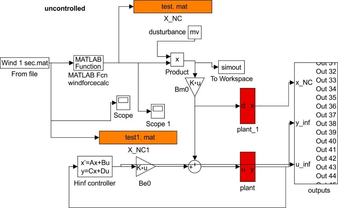
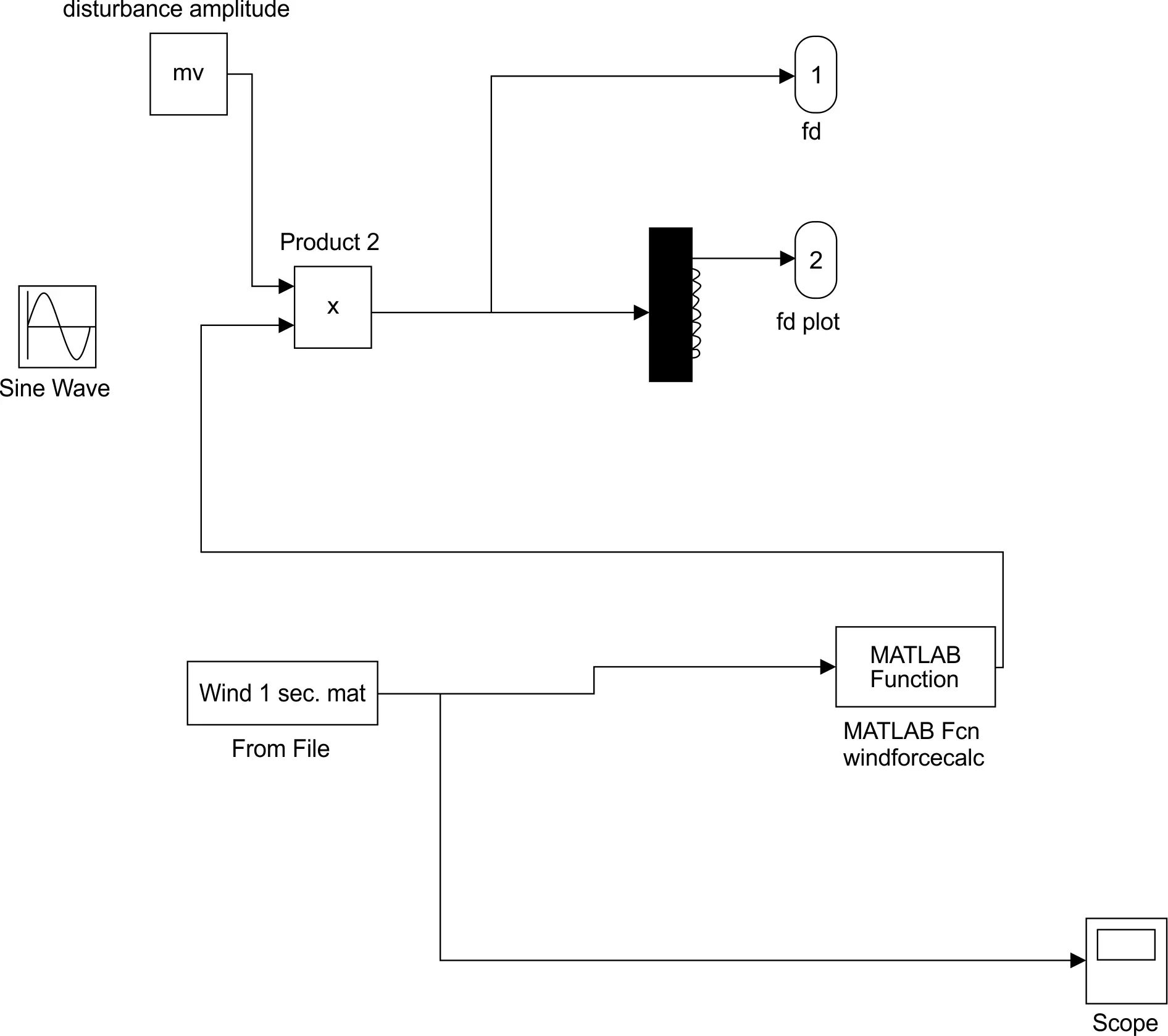
In the proposed method, the uncertainty of the original matrices is considered an additional measure of uncertainty. These equations capture the concept of dynamic loads or changing conditions being responded to by smart structures through active and flexible control. It is difficult to create control system algorithms that effectively confront the status of the structure and simultaneously address external forces (Figure 1).
3. Results
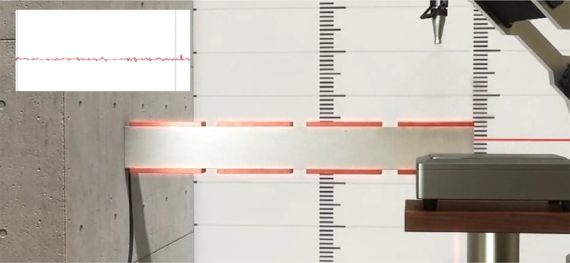
The cantilever smart structure (Figure 2) studied in this section features four pairs of symmetrically bonded piezoelectric patches. These were placed at the bottom and top of each beam element. The beam details are presented in Table 1.
Table 1. Features of the smart beam.
|
Parameters |
Values |
|---|---|
|
Wp, pzt Width, W, for Width of the beam |
0.003 m 0.003 m |
|
L, for beam length |
1.40 m |
|
hp, piezoelectric thickness h, for the thickness of the beam |
0.0002 m 0.096 m |
|
ρ, for Beam density |
1800 kg/m3 |
|
E, for the beam’s stiffness (Young’s modulus) |
1.7 × 10¹¹ N/m2 |
|
Ep, pzt Young’s modulus |
6.3 × 10¹⁰ N/m2 |
|
d31 the Piezoelectric constant |
250 × 10−12 m/V |
|
bs, ba, thickness of Pzt |
0.002 m |
Subheadings may be used to structure this section. It should offer a succinct and precise explanation of the experimental findings, their meanings, and any inferred experimental inferences. First, the nominal performance was created on the MATLAB software platform (v.6.5, MathWorks, Natick, MA, USA) (Figure 3 and Figure 4).
Next, uncertainty modeling was performed using Equation (6), Equation (7), Equation (8), Equation (9), Equation (10), Equation (11) and Equation (12), and the developed MATLAB code was applied to the data.
In the context of the results, the disturbance being a sinusoidal force suggests that the system is subjected to a periodic input, and the H∞ control is used to stabilize and optimize the system performance under this disturbance. To break down the description of the results and what Figure 5 represents, in the left diagram, matrices A and B (from Equation (12)) are analyzed with H∞ Control. Figure 5 illustrates the response of the system, focusing on the different elements of matrices A and B from Equation (12), which are likely to be parts of the state-space representation of the system. These matrices represent the system dynamics and control input relationships. H∞ Control Application: The left diagram shows the system behavior when H∞ control is applied to specific elements of matrices A and B. The middle diagram shows a system behavior comparison with and without the application of the control, and the (blue curve) depicts the results when the H∞ controller was applied. This line shows the response of the system when the robust controller is active, thereby demonstrating improved stability and reduced oscillations.
Without Control (Open-Loop System–Various Colors): The other lines in different colors represent the system response without control (open-loop). These uncontrolled responses are likely to be oscillatory or unstable, demonstrating the effect of sinusoidal disturbances on the system when corrective measures are not implemented in the control system.
The right-hand diagram illustrates the control voltages generated by the H∞ controller for the different outcomes of matrices A and B. These control voltages represent the control inputs (likely voltages applied to actuators or smart materials) required by the H∞ controller to stabilize the system in the presence of a given disturbance.
B was tested to observe the change in control effort (in terms of voltage). The goal is to ensure that the controller maintains stability and performance across different configurations of system dynamics (variations with A and B: different values or combinations of A and B).
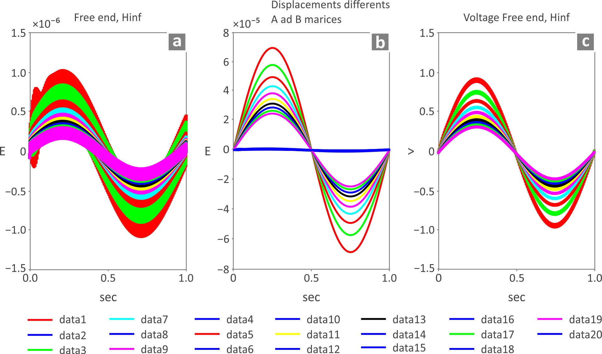
Figure 5. (a) Displacements with Hinfinity with different prices A and B, (b) Displacements without and with control with different values A, B, (c) Control Voltages with Hinfinity with different prices A and B.
|
```latex\begin{aligned} & \text{UNCERTAINTY Modeling} \\ & \\ & \%\,\,\,\text{uncertainty modeling} \\ & \mathrm{delta\_m = 10^{-5};}\\ &\mathrm{delta\_k = delta\_m^2;}\\ & \mathrm{\%\,\,\,delta\_d = delta\_m};\\ & \mathrm{\%\,\,\,Delta = \mathrm{eye}(3 \times nd);}\\ & \mathrm{X_m = mm1 \times delta\_m;}\\& \mathrm{X_k = kk1 \times delta\_k;}\\& \mathrm{X_d = 0.0005 \times (X_m + X_k);}\\& \\& \\ & \mathrm{G_{bar} = -[X_m\ X_d\ X_k]; }\\ & \mathrm{P_m = \mathrm{eye}(nd);}\\& \mathrm{P_k = \mathrm{eye}(nd);}\\& \mathrm{P_d = \mathrm{eye}(nd);}\\ &\\ & \mathrm{G_{bar0} = [ \mathrm{zeros}(nd, 3 \times nd)}; \\&\mathrm{ \mathrm{inv}M \times G_{bar}];} \\ & \mathrm{E_1 = [\,\,\, P_m \,\,\,\,\,\,\,\,\,\,\,\,\,\,\, \mathrm{zeros}(nd, nd); }\\&\mathrm{ \mathrm{zeros}(nd, nd) \,\,\,\,\,\,\,\, P_d };\\ &\mathrm{\mathrm{zeros}(nd, 2 \times nd)];}\\& \\& \mathrm{E_2 = [ \mathrm{zeros}(nd, 2 \times nd)} \\ &\mathrm{\mathrm{zeros}(nd, 2 \times nd)} \\& \mathrm{\mathrm{zeros}(nd, nd)\,P_k];} \\ &\\ &\%\,\,\, \mathrm{\text{from } d, n, p \text{ to uncertainty} }\\ & \mathrm{S{dq} = (E_1 + E_2 \times H)*\left(\mathrm{eye}(2 \times nd) - B_0 \times K \times C_0 \times H\right)^{-1} \times G_0 \times W_d;} \\ &\mathrm{ S{nq} = (E_1 + E_2 \times H)*\left(\mathrm{eye}(2 \times nd) - B_0 \times K \times C_0 \times H\right)^{-1} \times B_0 \times K \times W_n;} \\ &\mathrm{ S{pq} = (E_1 + E_2 \times H)*\left(\mathrm{eye}(2 \times nd) - B_0 \times K \times C_0 \times H\right)^{-1} \times {G}_{bar0};} \\ & \mathrm{S{pe} = W_e \times J \times H \times\left(\mathrm{eye}(2 \times nd) + B_0 \left(K \left(\mathrm{eye}(nd/2) - C_0 \times H \times B_0 \times K\right)^{-1} \times C_0 \times H\right)\right) \times {G}_{bar0}; }\\ & \mathrm{S{pu} = W_u \times K\times \left(\mathrm{eye}(nd/2) - C_0 \times H \times B_0 \times K\right)^{-1} \times C_0 \times H \times {G}_{bar0};} \\ & \mathrm{S{de} = W_e \times J \times H \times\left(\mathrm{eye}(2 \times nd) + B_0\times \left(K\times \left(\mathrm{eye}(nd/2) - C_0 \times H \times B_0 \times K\right)^{-1} \times C_0 \times H\right)\right) \times G_0 \times W_d;} \\ & \mathrm{S{ne} = W_e \times J \times H \times B_0 \times K\times \left(\mathrm{eye}(nd/2) - C_0 \times H \times B_0 \times K\right)^{-1} \times W_n;} \\ & \mathrm{S{du} = W_u \times K \times\left(\mathrm{eye}(nd/2) - C_0 \times H \times B_0 \times K\right)^{-1} \times C_0 \times H \times G_0 \times W_d;} \\ & \mathrm{S{nu} = W_u \times K \times\left(\mathrm{eye}(nd/2) - C_0 \times H \times B_0 \times K\right)^{-1} \times W_n;} \\ &\\ &\mathrm{ M = [ S{pq}\,S{dq} \, S{nq}}; \\&\mathrm{ S{pe} \, S{de} \, S{ne}; \text{mass and stiffness matrices}} \\& \mathrm{S{pu} \, S{du} \, S{nu} ];} \\ \end{aligned}``` |
|
Figure 5 shows a detailed analysis of the outcome of the smart system for sinusoidal disturbances with and without control. The H∞ controller significantly enhanced the robustness of the system by reducing oscillations and stabilizing the dynamic response, as illustrated in the middle diagram.
The mass (M) and stiffness (K) matrices from Equation (12) are the main focus of the H∞ control analysis of the system reaction to wind force disturbances, as shown in Figure 6. Under H∞ control, the graph on the left illustrates how the displacements change for various portions of the mass (M) and stiffness (K) matrices. This demonstrates how well the control handles these fluctuations, reduces the displacements, and stabilizes the system.
The displacements with and without control are compared in the central diagram. The system with H∞ control is indicated by the blue line, which indicates increased stability and fewer vibrations. The larger displacements of the colored lines (open-loop and no-control) highlight the effectiveness of the control in reducing the influence of wind disturbance.
The control voltages for various mass and stiffness levels are shown on the right side of the diagram. The voltages indicate the required amount of control for the system. The voltages indicate the amount of control that must be used to keep the objects stable under these changing circumstances. The findings demonstrate that the system maintains stability with minimal vibration in various configurations and that the control effort is tolerable. H∞ control, even with different masses and stiffnesses, often significantly minimizes vibrations and maintains stability. These results attest to the efficiency of the windbreaks in controlling wind disturbances.
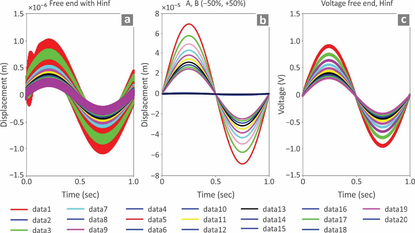
Figure 6. (a) Displacements with H infinity with different prices M and K, (b) Displacements with and without application of control with variable prices M, K, (c) Control Voltages with H infinity with variable prices M and K.
Regarding the subsequent collection of outcomes, where the disturbance is a wind force, Figure 7 offers insights into the system response under this new disturbance. The details of each section are presented in the figure. Left Diagram: Displacements for different elements belonging to matrices A and B (Equation (12)) with H∞ control. Figure 6 illustrates the displacements of the system for various elements of matrices A and B (which are part of the state-space equation representation in Equation (12)) under the influence of H∞ control. This refers to the extent to which the nodes in the smart structure (e.g., a smart beam) are displaced as a result of wind force disturbance. H∞ Control Impact: The left diagram shows how H∞ control manages the displacements of the different components for matrices A and B.
Middle Diagram: Displacements with and Without Control (open-loop versus closed-loop). The middle diagram in Figure 7 focuses on a comparison of displacements with and without control: With H∞ Control (Blue Line): The blue line represents the system’s displacements when H∞ control is applied. Here, the control system actively reduces the displacement caused by the wind force, leading to a more stable and predictable behavior.
Without Control (Open-Loop, Different Colors): Colored lines represent the system’s behavior without control (open-loop scenario). These lines likely show larger displacements or oscillatory behavior owing to wind disturbances, indicating a lack of stability and robustness in the open-loop system. Key Insight: This comparison demonstrates the efficiency of the H∞ control in reducing wind-induced displacements, clearly showing improved performance (less displacement) when the control is active compared with the open-loop case—right Diagram: Control Voltages with H∞ for different A and B values in the rightmost diagram. Figure 7 shows the control voltages required by the H∞ controller to maintain stability for varying values of matrices A and B. These voltages represent the inputs (possibly the voltages applied to the actuators or other control mechanisms) necessary to stabilize the system under wind-force disturbances.
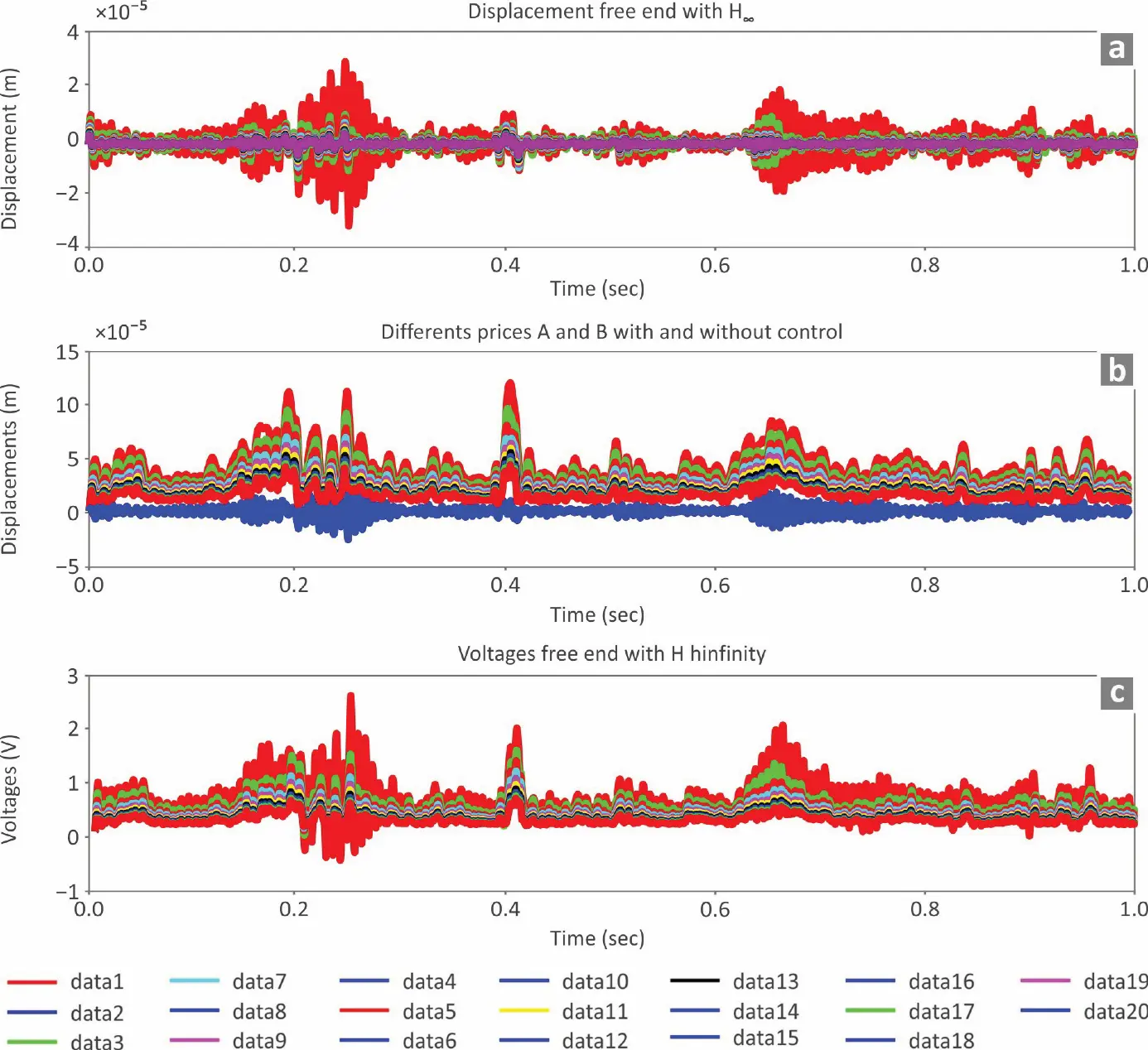
Figure 7. Wind force: (a) Displacements with H-infinity with different prices A and B, (b) Displacements with and without control with different prices A, B, (c) Control Voltages with Hinfinity with different prices A and B.
In Figure 8, the system response to the wind force disturbance is analyzed using H∞ control, focusing on the mass (M) and stiffness (K) matrices from Equation (12). The diagram on the left shows how the displacements vary for discrete parts of the stiffness and mass matrices under the H∞ control. The graphs above show that when the control method (H-infinity) was implemented, the system showed an increase in stability as well as a decrease in displacements owing to the control of the vibrations caused by the disturbance (wind). The graph on the left shows two lines: one with the application of control (blue) and one without (red). The blue line shows a smaller displacement compared to the red line, which has a larger displacement. There was a clear risk that applying the control would give an unstable result, as measured in a comparison of the response magnitudes of the systems with and without control due to the disturbance (wind). However, based on the results from simulations with varying stiffness and mass values of the system, the graph on the right shows the control voltages required to keep the system stable. The amount of control required to achieve the response was very low, and the system was able to remain stable with very little vibration across all configurations tested.
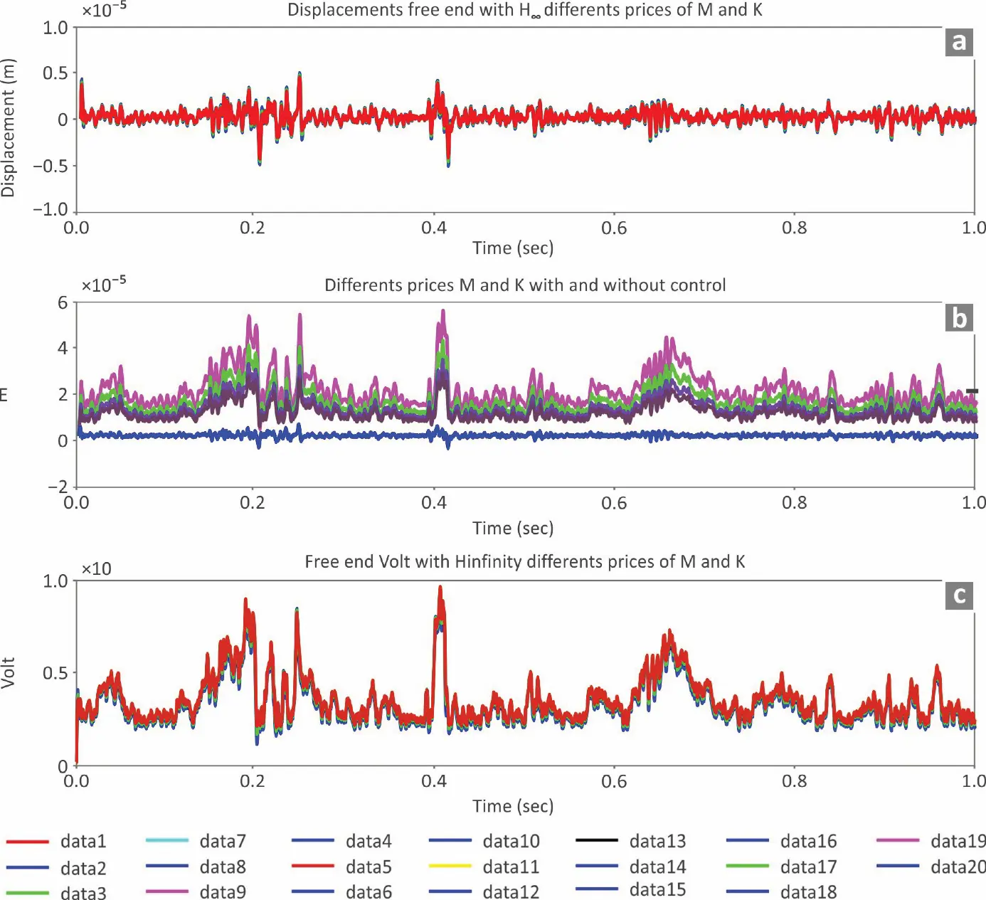
Figure 8. Wind force: (a) Displacements with Hinfinity with different prices M, K, (b) Displacements with and without application of control with different values for M, K, (c) Control Voltages with Hinfinity with different prices M and K.
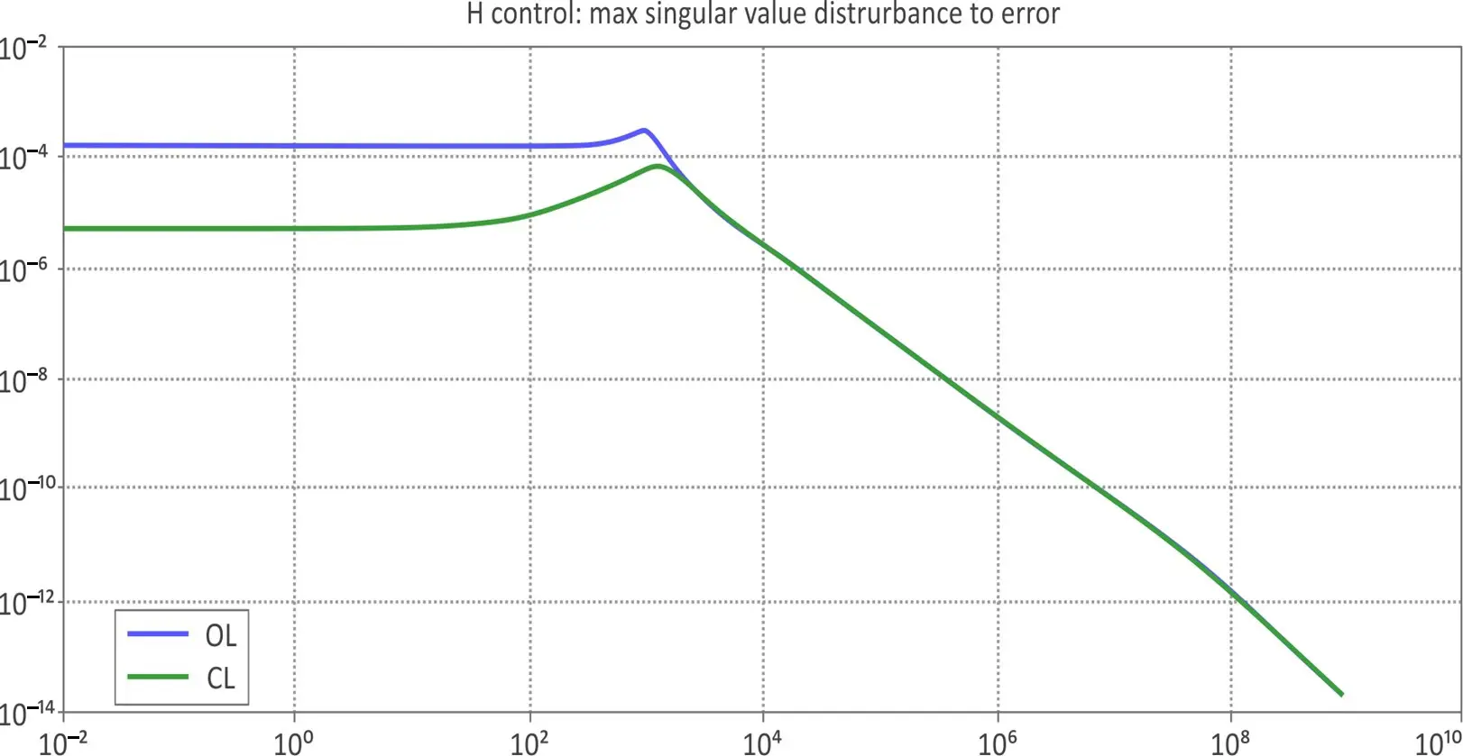
In conclusion, the H-infinity controller is a viable means of stabilizing the system and significantly reducing the amount of displacement experienced during a disturbance (i.e., wind). To validate the time-domain results, plots of both the closed- and open-loop systems for the frequency-frequency view were created, as shown in Figure 9. The singular value of the system was calculated as the effect of a disturbance, that is, the error. The influence of Αn was monitored. In particular, a significant improvement in perturbation inaccuracy was observed up to a frequency of 1000 Hz.
Reducing vibrations is a fundamental problem for engineers, and creating sustainably optimized structures is important. In conclusion, this study achieves the following:
-
Complete suppression of the oscillations. With the control, E was reduced from almost 6.0 × 10⁻⁵ to less than 0.5 × 10⁻⁵, while the displacement in meters was reduced from almost 10−4 to less than 3.0 × 10⁻⁵.
-
Introduction of uncertainty in the simulation model.
-
Application of advanced control techniques to smart structures.
-
Creation of optimal and sustainable structures.
-
Control of structures in both the time and frequency domains.
-
Modeling of the structure through algorithms and the introduction of dynamic loads.
-
The results for various types of dynamic loads were examined, considering noise and modeling errors.
4. Discussion
This study presents advances in the intelligent control of sustainable structures. The goal of this study is to create sophisticated control strategies to suppress oscillations and intelligently regulate the piezoelectric structures. The creation of sophisticated control algorithms is a significant accomplishment. The development of Adaptive Control Techniques has been made possible by the time-varying characteristics of piezoelectric materials [10,32,33]. This study provides insight into the development of methods to reduce oscillations caused by variations in mass and stiffness (matrix stiffness) arising from various modeling methods and/or structural damage that may result from varying the initial conditions of the system. Two control strategies were used to suppress the oscillations caused by variations in the initial conditions of the system. Both exhibited robust performances, meaning that despite facing unexpected conditions (uncertainties and structural anomalies), re-stabilization and suppression of oscillations were achieved.
Because piezoelectric materials were added to the original structures, the study reported in this paper shows how resilient control techniques can improve the dependability and efficiency of intelligent structures. It has been demonstrated that resilient controls based on the H-infinity (H∞) technique are very successful in suppressing vibrations while preserving system stability over variations in mass and stiffness. Additionally, H∞ controllers can manage wind-induced disruptions, enabling steady and efficient operation. The development of a sophisticated technique for controlling the oscillations of global piezoelectric structures will impact intelligent structural control.
Although the control methods described will change how the initial conditions are defined for a system, the proposed methods are capable of effectively minimizing oscillations and thereby producing stable motion. A significant characteristic of the results presented in this section is their robustness to variations in parameter values, which demonstrates that the proposed methods can maintain the controllability and stability of the system for a much wider range of initial conditions than when these methods are not used. The ability to create damping in the oscillation response of the system to varying initial conditions is a critical aspect of the reliability and robustness of the system, ensuring that it functions according to its intended performance level. Furthermore, given the potential for a number of uncertainties and modeling errors to occur in real-world applications, the evidence provided by the results presented in this study provides valuable insights into the potential implications of these uncertainties on the long-term performance and operational viability of the system, as described.
The controller offers numerous advantages: the system exhibits exceptional disturbance rejection and is robust in the presence of noise and oscillations. Furthermore, it illustrates how a reduced controller order can achieve enhanced efficiency without substantially compromising the performance. The use of intelligent controls to reduce structural vibrations by employing various state-of-the-art technologies and methods has advanced in recent years. In addition to producing contemporary structures that support sustainable growth, piezoelectric materials can reduce vibrations. To reduce vibrations, several researchers have employed active control techniques. Active control systems employ sensors and actuators to respond to vibrations dynamically. The creation of Smart Structures and Materials is a significant advancement in this field.
5. Conclusions
In conclusion, this study presents innovations in the modeling of new sustainable structures that use new modern materials and smart systems. These structures, in order to operate, use advanced control techniques developed analytically in this study. The features of this study illustrate a reduction in oscillations through the recording of stiffness. This indicates deviations from the initial conditions of the system, which may be indicative of modeling errors or structural damage. This is perceptually configured with the damping of oscillations under variable initial conditions. This study recommends employing robust and operational modeling for system design analysis. Intelligent structures that utilize piezoelectric materials must possess disturbance rejection properties. The capability to design a system with disturbance rejection properties and data logging capabilities using a reliable and accurate version of MATLAB proved to be a valuable platform for modeling and simulating intelligent systems. The state-space simulation employed in this study was designed to develop and implement an H-infinity controller to compare the advantageous attributes of resilient control using disturbance variable recordings, as exemplified in the preceding chapters. Innovations in the modeling of new sustainable structures that use smart materials and intelligent structures are presented in this study. These structures employ robust control strategies that are theoretically defined in this study in order to function. The controller has several benefits, such as the remarkable rejection of disturbances and resilience to oscillations and noise. It also shows how improved efficiency may be attained with a lower controller order without significantly sacrificing the performance. In recent years, advancements have been made in the application of intelligent controls to reduce structural vibrations using various cutting-edge technologies and techniques. Piezoelectric materials can not only create modern buildings that promote sustainable growth but also reduce vibrations. The innovation of this study is that it uses advanced control techniques that consider the optimization of construction by reducing oscillations and measurement noise. These techniques optimize construction by considering modeling uncertainties. The construction process becomes optimal and sustainable.
Author Contributions
A.M. and M.P.: software, formal analysis, writing review, and editing; G.E.S.: methodology; A.P.: investigation and software; N.V.: validation. All authors have read and agreed to the published version of this manuscript.
Ethics Statement
Not applicable.
Informed Consent Statement
Not applicable.
Data Availability Statement
The authors confirm that the data supporting the findings of this study are available in this article.
Funding
This research received no external funding.
Declaration of Competing Interest
The authors declare that they have no known competing financial interests or personal relationships that could have appeared to influence the work reported in this paper.
References
-
Chandrashekhara K, Varadarajan S. Adaptive Shape Control of Composite Beams with Piezoelectric Actuators. J. Intell. Mater. Syst. Struct. 1997, 8, 112–124. DOI:10.1177/1045389X9700800202 [Google Scholar]
-
Bona B, Indri M, Tornambe A. Flexible Piezoelectric Structures-Approximate Motion Equations and Control Algorithms. IEEE Trans. Automat. Contr. 1997, 42, 94–101. DOI:10.1109/9.553691 [Google Scholar]
-
Bandyopadhyay B, Manjunath TC, Umapathy M. Modeling, Control and Implementation of Smart Structures: A FEM-State Space Approach; Springer: Berlin/Heidelberg, Germany, 2007; ISBN 978-3-540-48393-9. [Google Scholar]
-
Choi S-B, Cheong C-C, Lee C-H. Position Tracking Control of a Smart Flexible Structure Featuring a Piezofilm Actuator. J. Guid. Control. Dyn. 1996, 19, 1364–1369. DOI:10.2514/3.21795 [Google Scholar]
-
Davim JP. Vibration: A Bibliometric Analysis. Sound Vib. 2025, 59, 2627. DOI:10.59400/sv2627 [Google Scholar]
-
Davim JP. Sustainable and Intelligent Manufacturing: Perceptions in Line with 2030 Agenda of Sustainable Development. Bioresources 2024, 19, 4. DOI:10.15376/biores.19.1.4-5 [Google Scholar]
-
Davim JP. Sustainable Manufacturing; John Wiley & Sons: Hoboken, NJ, USA, 2013. [Google Scholar]
-
Davim JP. Perceptions of Industry 5.0: Sustainability Perspective. Bioresources 2025, 20, 15. DOI:10.15376/biores.20.1.15-16 [Google Scholar]
-
Culshaw B. Smart Structures—A Concept or a Reality? Proc. Inst. Mech. Eng. Part I: J. Syst. Control. Eng. 1992, 206, 1–8. DOI:10.1243/PIME_PROC_1992_206_302_02 [Google Scholar]
-
Doyle J, Glover K, Khargonekar P, Francis B. State-Space Solutions to Standard H2 and H∞ Control Problems. In Proceedings of the 1988 American Control Conference, Atlanta, GA, USA, 15–17 June 1988; pp. 1691–1696. [Google Scholar]
-
Tzou HS, Gabbert U. Structronics—A New Discipline and Its Challenging Issues. Fortschr.-Berichte VDI Smart Mech. Syst.—Adapt. Reihe 1997, 11, 245–250. [Google Scholar]
-
Guran A, Tzou H-S, Anderson GL, Natori M, Gabbert U, Tani J, et al. Structronic Systems: Smart Structures, Devices and Systems; World Scientific: Singapore, 1998; Volume 4; ISBN 978-981-02-2652-7. [Google Scholar]
-
Tzou HS, Anderson GL. Intelligent Structural Systems; Springer: Dordrecht, The Netherlands, 1992; ISBN 978-94-017-1903-2. [Google Scholar]
-
Gabbert U, Tzou HS. IUTAM Symposium on Smart Structures and Structronic Systems: Proceedings of the IUTAM Symposium Held in Magdeburg, Germany, 26–29 September 2000; Springer: Berlin/Heidelberg, Germany, 2001. [Google Scholar]
-
Tzou HS, Natori MC. Piezoelectric Materials and Continua. In Encyclopedia of Vibration; Braun S, Ed.; Elsevier: Oxford, UK, 2001; pp. 1011–1018; ISBN 978-0-12-227085-7. [Google Scholar]
-
Cady WG. Piezoelectricity: An Introduction to the Theory and Applications of Electromechanical Phenomena in Crystals; Courier Dover Publication: New York, NY, USA, 1964. [Google Scholar]
-
Tzou HS, Bao Y. A Theory on Anisotropic Piezothermoelastic Shell Laminates with Sensor/Actuator Applications. J. Sound Vib. 1995, 184, 453–473. DOI:10.1006/jsvi.1995.0328 [Google Scholar]
-
Moutsopoulou A, Stavroulakis GE, Petousis M, Vidakis N, Pouliezos A. Smart Structures Innovations Using Robust Control Methods. Appl. Mech. 2023, 4, 856–869. DOI:10.3390/applmech4030044 [Google Scholar]
-
Cen S, Soh AK, Long YQ, Yao ZH. A New 4-Node Quadrilateral FE Model with Variable Electrical Degrees of Freedom for the Analysis of Piezoelectric Laminated Composite Plates. Compos. Struct. 2002, 58, 583–599. DOI:10.1016/S0263-8223(02)00167-8 [Google Scholar]
-
Yang SM, Lee YJ. Optimization of Noncollocated Sensor/Actuator Location and Feedback Gain in Control Systems. Smart Mater. Struct. 1993, 2, 96–102. DOI:10.1088/0964-1726/2/2/005 [Google Scholar]
-
Ramesh Kumar K, Narayanan S. Active Vibration Control of Beams with Optimal Placement of Piezoelectric Sensor/Actuator Pairs. Smart Mater. Struct. 2008, 17, 55008. DOI:10.1088/0964-1726/17/5/055008 [Google Scholar]
-
Hanagud S, Obal MW, Calise AJ. Optimal Vibration Control by the Use of Piezoceramic Sensors and Actuators. J. Guid. Control. Dyn. 1992, 15, 1199–1206. DOI:10.2514/3.20969 [Google Scholar]
-
Song G, Sethi V, Li H-N. Vibration Control of Civil Structures Using Piezoceramic Smart Materials: A Review. Eng. Struct. 2006, 28, 1513–1524. DOI:10.1016/j.engstruct.2006.02.002 [Google Scholar]
-
Bosgra OH, Kwakernaak H, Meinsma G. Design Methods for Control Systems. Course Notes Dutch Inst. Syst. Control. 2001, 67. Available online: https://www.researchgate.net/profile/Stephen-Poon-5/post/How_many_methods_exists_for_designing_SM_control/attachment/59ea2f21b53d2fe117b7a6ad/AS%3A551585811046400%401508519713040/download/Design+Methods+for+Control+Systems.pdf (accessed on 20/12/2025).
-
Miara B, Stavroulakis GE, Valente V. Topics on Mathematics for Smart Systems: Proceedings of the European Conference, Rome, Italy, 26–28 October 2006; World Scientific: Singapore, 2007. [Google Scholar]
-
Moutsopoulou A, Stavroulakis GE, Pouliezos A, Petousis M, Vidakis N. Robust Control and Active Vibration Suppression in Dynamics of Smart Systems. Inventions 2023, 8, 47. DOI:10.3390/inventions8010047 [Google Scholar]
-
Zhang N, Kirpitchenko I. Modelling Dynamics of a Continuous Structure with a Piezoelectric Sensoractuator for Passive Structural Control. J. Sound Vib. 2002, 249, 251–261. DOI:10.1006/jsvi.2001.3792 [Google Scholar]
-
Zhang X, Shao C, Li S, Xu D, Erdman AG. Robust H∞ Vibration Control for Flexible Linkage Mechanism Systems with Piezoelectric Sensors and Actuators. J. Sound Vib. 2001, 243, 145–155. DOI:10.1006/jsvi.2000.3413 [Google Scholar]
-
Packard A, Doyle J, Balas G. Linear, Multivariable Robust Control With a μ Perspective. J. Dyn. Syst. Meas. Control 1993, 115, 426–438. DOI:10.1115/1.2899083 [Google Scholar]
-
Kwakernaak H. Robust Control and H∞-Optimization—Tutorial Paper. Automatica 1993, 29, 255–273. DOI:https://doi.org/10.1016/0005-1098(93)90122-A [Google Scholar]
-
Benjeddou A, Trindade MA, Ohayon R. New Shear Actuated Smart Structure Beam Finite Element. AIAA J. 1999, 37, 378–383. DOI:10.2514/2.719 [Google Scholar]
-
Kimura H. Robust Stabilizability for a Class of Transfer Functions. IEEE Trans. Automat. Contr. 1984, 29, 788–793. DOI:10.1109/TAC.1984.1103663 [Google Scholar]
-
Francis BA. A Course in H∞ Control Theory; Springer: Berlin/Heidelberg, Germany, 1987; ISBN 978-3-540-17069-3. [Google Scholar]