Integrated Assessment of Ecosystem Carbon Storage and Ecological Risk Index Under Multi-Objective Driven Approach: A Case Study of the Karst Ecologically Fragile Area in Guangxi

Integrated Assessment of Ecosystem Carbon Storage and Ecological Risk Index Under Multi-Objective Driven Approach: A Case Study of the Karst Ecologically Fragile Area in Guangxi
Hong Jiang 1 Feili Wei 1,2,* Jing Jing 1 Dahai Liu 3 Zhantu Chen 1 Ling Xie 1 Yu Jiang 1 Yuan Xu 1
Received: 27 December 2025 Revised: 13 March 2026 Accepted: 02 April 2026 Published: 16 April 2026

© 2026 The authors. This is an open access article under the Creative Commons Attribution 4.0 International License (https://creativecommons.org/licenses/by/4.0/).
1. Introduction
In recent years, global climate change has attracted increasing attention. The profound threat posed by global warming to both human living environments and public health has made it one of the most critical challenges of the 21st century [1]. In response, China has proposed the ‘dual carbon’ goals of peaking carbon emissions by 2030 and achieving carbon neutrality by 2060 [2,3], and is actively promoting a green and low-carbon transition through energy conservation, emissions reduction, industrial restructuring, and enhancement of ecosystem carbon sequestration capacity. Among these efforts, improving ecosystem carbon storage (CS) is considered a crucial strategy for mitigating climate change. According to the Intergovernmental Panel on Climate Change (IPCC) reports, land use/land cover change (LUCC) is a major factor influencing terrestrial CS (IPCC, 2022). Different land use types exhibit significant variability in carbon sequestration capacity, making LUCC a core pathway for regulating regional carbon sinks.
To effectively navigate the spatial trade-offs between carbon mitigation and regional development under future uncertainties, projecting these land use dynamics and their long term ecological impacts has become imperative [4,5]. Driven by this necessity, numerous studies have investigated the impact of LUCC on CS using various scales and simulation approaches, including Markov chains [6], system dynamics models [7], cellular automata (CA) [8], and multivariate statistical methods [9]. The PLUS (Patch-generating Land Use Simulation) model has gained widespread application in regional scale land use dynamic simulations in recent years due to its advantages in capturing spatial heterogeneity and detailing land type transitions in detail. It builds on CA-Markov and Random Forest approaches but adds two key components: a rule mining step that learns the drivers of expansion for each land use class, and a patch-growth module that propagates change as contiguous areas rather than scattered pixels [10,11]. Meanwhile, CS estimation has gradually shifted from traditional field-based poin-scale observations to model-based spatial estimation using land use structures and carbon density parameters. Among these models, InVEST (Integrated Valuation of Ecosystem Services and Trade-offs) has become one of the mainstream tools for regional CS estimation and ecosystem service assessment due to its simplicity and spatial simulation capabilities [12,13,14,15]. Recently, an increasing number of researchers have coupled the PLUS and InVEST models to assess the impact of LUCC on the spatial distribution and evolution of CS under different land use scenarios. This integrated approach has enriched the theoretical framework for dynamic simulation and prediction of ecosystem CS [16,17,18], as well as facilitating the scenario-based evaluation of forest carbon sequestration dynamics over extended periods [19].
While these dynamic simulations provide valuable insights into carbon sinks, robust landscape management further requires anticipating climate-driven degradation, soil erosion, and ecological reversal risks [20,21]. As the economic and ecological costs of multiple disturbances rise, mapping these large-scale threat regimes has become a critical necessity for preserving carbon sequestration capabilities [22,23]. Furthermore, recognizing the technological scopes and geological carbon storage constraints of engineered carbon capture and geologic storage [24,25], nature-based carbon sinks must be synergized with land use policies to collaboratively reduce pollution and carbon emissions in comprehensive environmental policymaking [26]. On the other hand, landscape ecological risk assessment, an important means of measuring regional ecological vulnerability, emphasizes the spatial responses of landscape pattern changes and ecological process disturbances under multisource pressures [27,28,29,30]. Relevant studies have mainly focused on ecologically sensitive areas such as coastal zones, mining regions, agropastoral ecotones, watersheds, and urban fringes. By integrating remote sensing data and geostatistical methods, multi-dimensional and multi-indicator ecological risk index systems have been constructed, enabling the quantitative and spatial visualization of regional ecological risks [31,32,33]. To operationalize these concepts, current macro-spatial and urban planning frameworks are actively incorporating scenario analyses to navigate the complex trade-offs among carbon storage, biodiversity, and spatial disturbance risks [34,35,36].
However, current research on the integrated assessment of landscape ecological risk and CS still faces two key limitations: first, most studies are conducted at small spatial scales, with a lack of systematic assessments of spatial coupling between CS and ecological risk at the provincial or large-scale ecosystem level; second, dynamic trade-off analyses under multiple development scenarios are insufficient, limiting their applicability in informing land use optimization and ecological conservation strategies under future development pathways.
To address these gaps, this study adopts the ecologically fragile karst region of Guangxi as a case study, integrating the PLUS and InVEST models within a multi-scenario framework to bridge a critical divide: generating spatially explicit, comparable carbon storage estimates that are directly tied to modeled land use pathways. Therefore, we simulate land use changes in 2030 under three scenarios (natural development, economic development, and ecological protection) and systematically assess the spatial evolution of ecosystem CS and the distribution of landscape ecological risks under each scenario. Guangxi is chosen for two main reasons. First, it is one of the provinces in China with the most extensive karst distribution. The region faces significant ecological challenges, including shallow soil layers, severe soil erosion, pronounced risks of rocky desertification, and a dual surface-subsurface hydrological system that exacerbates difficulties in vegetation restoration, resulting in marked spatial heterogeneity in ecosystem CS capacity. Second, rapid industrialization and urban expansion in recent years have intensified landscape fragmentation, with CS loss and ecological risk becoming increasingly coupled, heightening the conflict between development and conservation. Therefore, conducting a multi-scenario simulation-based integrated assessment of ecosystem CS and ecological risk under the unique ecological and geological background of karst regions holds significant scientific value. It also offers practical guidance for land use planning, ecological protection, and carbon sink management in Guangxi and other ecologically fragile karst regions.
2. Materials and Methods
2.1. Study Area
The study area is located in the Guangxi Zhuang Autonomous Region of China (20°54′–26°24′ N, 104°26′–112°04′ E), characterized by a topography that generally slopes from the highlands in the northwest to the lowlands in the southeast (Figure 1). The region features a diverse and transitional landscape composed of mountains, hills, basins, and coastal plains. Guangxi is one of China’s regions with the most extensive karst landforms, where the ecosystem is highly fragile due to shallow soils, severe soil erosion, and widespread rocky desertification. These factors substantially limit the carbon sink capacity of the region and lead to pronounced spatial heterogeneity in CS. In recent years, rapid urban expansion has dramatically altered land use patterns across Guangxi, exacerbating landscape fragmentation and elevating ecological risks. As a result, ecosystem CS is under increasing pressure. As a key region for implementing China’s dual carbon strategy, Guangxi has actively promoted the development of clean energy and pursued a green, low-carbon transition. However, significant trade-offs exist between new energy development and ecological protection, posing challenges to sustainable land use planning. Therefore, selecting a representative ecologically fragile karst area in Guangxi to assess CS changes and ecological risk distribution under different land use scenarios is of great theoretical and practical significance. The results can provide scientific guidance for optimizing regional land use, enhancing carbon sink functions, and improving ecosystem stability.
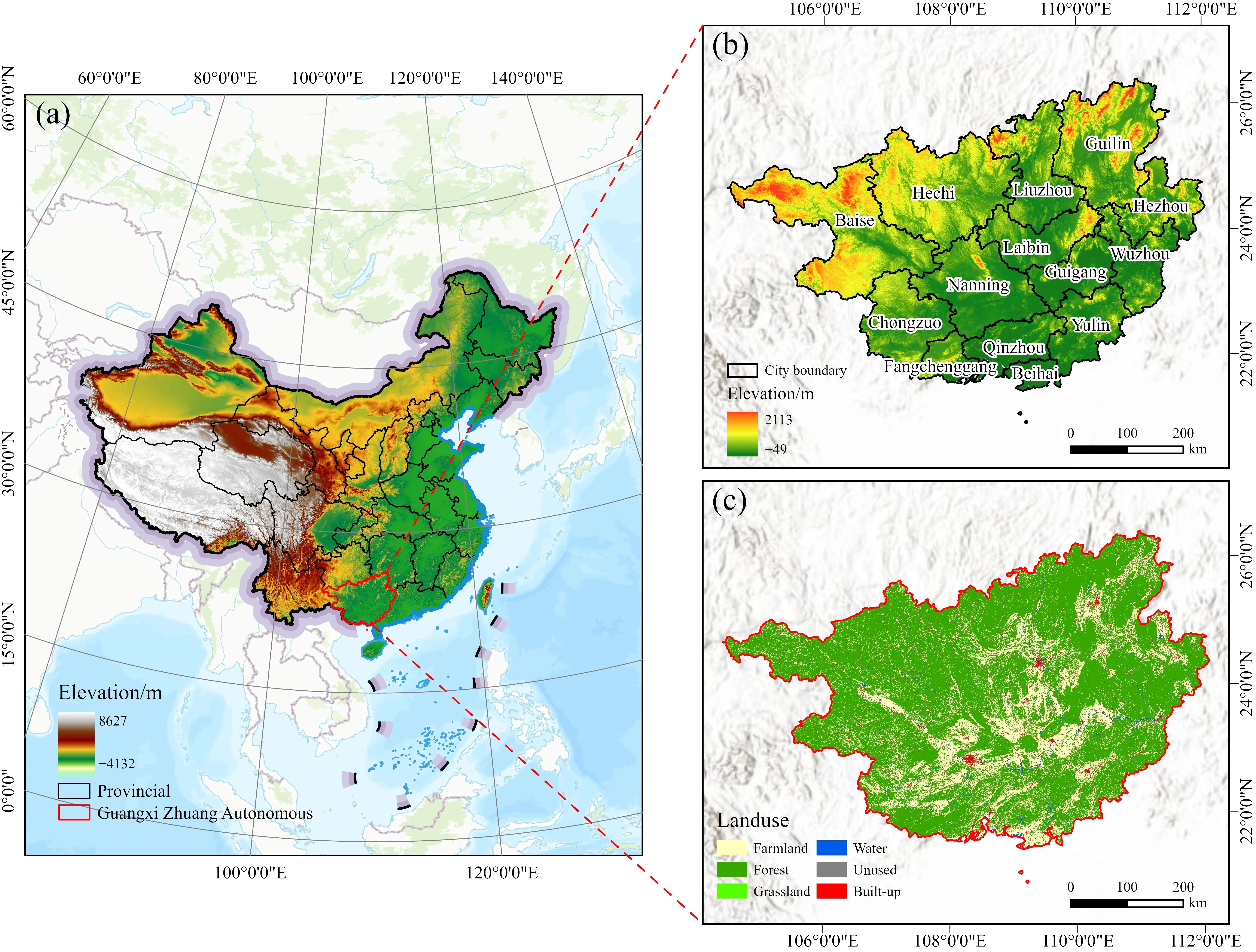
Figure 1. Overview of the study area. Notes: (a) Location of the study area; (b) Digital Elevation Model (DEM) of the study area; (c) Land use/land cover (LULC) map of the study area in 2020. The map was created using a standard base map (Map Approval No. GS (2024)0650) obtained from the National Geographic Information Public Service Platform. No modifications were made to the original map.
2.2. Data Sources
The data used in this study include LUCC and a set of driving factors. The LUCC were obtained from the national land cover dataset provided by Yang and Huang [37], with a spatial resolution of 30 m. The driving factors consist of both natural and socioeconomic variables. All raster layers were standardized to 30 m resolution by resampling and clipping; the land use layer was aligned to the common grid so that all datasets share the same projection and dimensions. Detailed information on all datasets is presented in Table 1.
Table 1. Data sources.
|
Data Type |
Data Name |
Resolution/m |
Data Sources |
|---|---|---|---|
|
Natural factors |
Soil type |
30 |
https://soil.geodata.cn/ (accessed on 18 July 2025) |
|
DEM |
30 |
https://www.gscloud.cn/ (accessed on 18 July 2025) |
|
|
Slope |
30 |
Extracted from DEM data (http://www.gscloud.cn/ accessed on 18 July 2025) |
|
|
Annual average temperature (TEM) |
1000 |
https://data.cma.cn/ (accessed on 18 July 2025) |
|
|
Annual average precipitation (PRE) |
1000 |
||
|
Socio-economic factors |
Population (POP) |
1000 |
https://www.resdc.cn/ (accessed on 18 July 2025) |
|
GDP |
1000 |
||
|
Distance to roads |
1000 |
https://www.webmap.cn/ (accessed on 18 July 2025) |
|
|
Distance to railways |
1000 |
||
|
Distance to municipal government |
1000 |
||
|
Distance to rivers |
1000 |
2.3. Methodology
Figure 2 illustrates the research framework, which comprises three primary components. The first component involves data preparation and processing, including the LUCC dataset, data on 11 driving factors, and relevant land use policies in Guangxi. The second component uses the PLUS model to simulate land use patterns in Guangxi for the year 2030 under three scenarios: the Natural Development (ND) scenario, the Economic Development (ED) scenario and the Ecological Protection (EP) scenario. The third component applies the Landscape Ecological Risk Index and spatial autocorrelation analysis to assess the spatiotemporal variation in the Ecological Risk Index (ERI). The specific research methods involved in this study are detailed as follows.
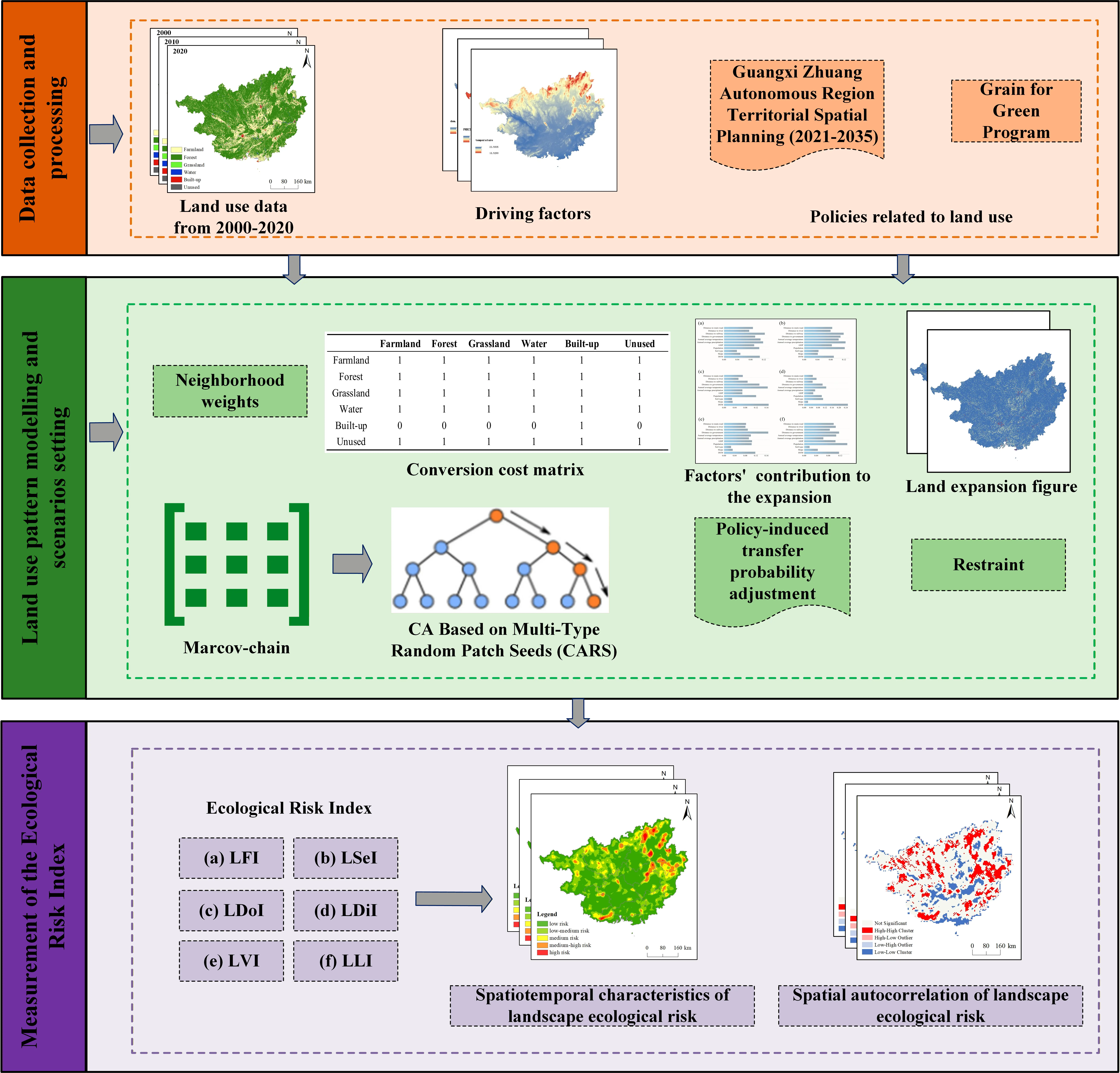
Figure 2. Research framework. Notes: (a) LFI, Landscape Fragmentation Index; (b) LSeI, Landscape Separation Index; (c) LDoI, Landscape Dominance Index; (d) LDiI, Landscape Disturbance Index; (e) LVI, Landscape Vulnerability Index; (f) Landscape Loss Index.
2.3.1. Land Use Dynamic Degree
The land use dynamic degree (LUDD) can reflect the intensity of land use change within a region. It can be categorized into single dynamic degree (SDD) and comprehensive dynamic degree (CDD) [38]. In this study, the SDD is adopted to quantitatively reveal the spatial and temporal intensity of land use changes in Guangxi. The calculation formula is presented in Equation (1):
|
```latexK=\frac{{U}_{b}-{U}_{a}}{{U}_{a}}×\frac{1}{T}×100\%``` |
(1) |
where K represents LUDD for a specific land use type within the study area. The magnitude of K indicates the rate or intensity of change in land use, while its sign (positive or negative) reflects the direction of change, whether the land area has increased or decreased. Ua and Ub refer to the land area of a certain land use type at the beginning and end of the study period, respectively. T denotes the length of the time interval (in years) over which the change is observed. In this study, T is set to 10 and 20 years, representing both short-term and long-term periods of analysis.
2.3.2. Construction of the Landscape Ecological Risk Assessment Model
Landscape indices can be used individually or in combination to analyze the spatial structure and evolutionary characteristics of landscapes. Incorporating landscape structure into an ecological risk assessment framework enables a more comprehensive evaluation of regional ecological conditions [39]. In this study, a landscape ecological risk assessment model was constructed based on the area proportions of different land use types and selected landscape pattern indices [40]. Following the principle of using 2–5 times the average patch area, and considering the actual landscape characteristics observed in the field, the study area was divided into grid cells of 5 km × 5 km [41]. By overlaying the classified land use data with the grid, the ecological risk index (ERI) for each cell was calculated and assigned to the centroid of the corresponding sample unit for interpolation analysis.
Six indices were selected to build the ecological risk index model: landscape fragmentation index ($${C}_{i}$$), landscape separation index ($${N}_{i}$$), landscape dominance index ($${D}_{i}$$), landscape disturbance index ($${S}_{i}$$), landscape vulnerability index ($${F}_{i}$$), and landscape loss index ($${R}_{i}$$). These indices were combined in the construction of the ecological risk index, as shown in Equation (2). Detailed formulas and parameter definitions for each index are provided in Table 2.
Table 2. Descriptions of landscape indices in the ecological risk assessment model.
|
Index |
Formula |
Ecological Significance |
|---|---|---|
|
Landscape fragmentation index ($${{C}}_{{i}}$$) |
```latex{{C}}_{{i}}{ }{=}{ }\frac{{{n}}_{{i}}}{{{A}}_{{i}}}``` |
It represents the degree of landscape fragmentation after segmentation, where $${{n}}_{{i}}$$ is the number of patches of landscape type i, and $${{A}}_{{i}}$$ is the total area of landscape type i. |
|
landscape separation index$${{ (}{N}}_{{i}}{)}$$ |
```latex{{N}}_{{i}}{ }{=}{ }\frac{{1}}{{2}}\sqrt{\frac{{{n}}_{{i}}}{{{A}}_{{i}}}}{×}\frac{{A}}{{{A}}_{{i}}}``` |
It represents the degree of separation among individual patches of a certain landscape type. In the formula, A denotes the total landscape area. |
|
landscape dominance index$${{ (}{D}}_{{i}}{)}$$ |
```latex{{D}}_{{i}}{ }{=}{ }\frac{{{M}}_{{i}}}{{2}}{ }{+}{ }\frac{{{L}}_{{i}}}{{2}}``` |
It represents the importance of a certain type of patch within the landscape. In the formula, $${{M}}_{{i}}$$ is the number of patches of type $${i}$$ divided by the total number of patches, and $${{L}}_{{i}}$$ is the total area of patches of type $${i}$$ divided by the total landscape area. |
|
landscape disturbance index ($${{S}}_{{i}}{)}$$ |
```latex{{S}}_{{i}}{ }{=}{ }{a}{{C}}_{{i}}{ }{+}{ }{b}{{N}}_{{i}}{ }{+}{ }{c}{{D}}_{{i}}``` |
It represents the degree to which ecosystems represented by different landscape types are affected by human activities. In the formula, a, b and c are the weights assigned to the corresponding landscape indices, with the constraint a + b + c = 1. Based on previous studies and practical considerations, the weights are set as a = 0.5, b = 0.3 and c = 0.2 [42]. |
|
landscape vulnerability index ($${{F}}_{{i}}{)}$$ |
Scores were assigned based on expert evaluation and then normalized |
The sensitivity of various landscape types to external disturbances was quantified using a numerical index. The assigned values are: unused land (6), water bodies (5), cultivated land (4), grassland (3), forest land (2) and construction land (1). These values were then normalized to obtain the landscape vulnerability index. |
|
landscape loss index ($${{R}}_{{i}}{)}$$ |
```latex{{R}}_{{i}}{ }{=}{ }\sqrt{{{S}}_{{i}}{×}{{F}}_{{i}}}``` |
It represents the degree of loss in the natural attributes of ecosystems represented by different landscape types when subjected to natural and human disturbances. |
The calculation formula for the Landscape Ecological Risk Index, based on the Loss Degree Index and landscape area, is shown in Equation (2):
|
```latexER{I}_{k}=\sum _{i=1}^{n}\frac{{A}_{ki}}{{A}_{k}}×{R}_{i}``` |
(2) |
where ERIk denotes the landscape ecological risk index; n corresponds to the total number of discrete land cover types present within the study extent; Aki signifies the area occupied by the i-th landscape class in the k-th assessment unit; and Ak represents the overall area of that assessment unit. Ri represents the landscape loss index of land-use type i.
2.3.3. Land Use Change Prediction Analysis
This study primarily employs the PLUS model to simulate land use change characteristics under different scenarios. The main advantage of the PLUS model lies in its integration of rule-mining methods with the Cellular Automata (CA) model, combined with various random seed mechanisms [43]. Based on this model, the study first identifies areas of land use expansion between two time periods and conducts sampling analysis on the newly added parts. Subsequently, random forest techniques are used to assess the growth probability of each land use type and evaluate the influence of driving factors on these expansions. Finally, future land use maps are automatically generated according to the CA model simulation.
To ensure the practical relevance of the results, three distinct land use scenarios are established: ND, ED, and EP. The constraints, such as ecological spaces, cultivated land protection boundaries, and urban expansion limits in each scenario are primarily set based on threshold values outlined in the ‘14th Five-Year Plan for Ecological Environment Protection of Guangxi’ and the ‘Guangxi Zhuang Autonomous Region Territorial Spatial Planning (2021–2035)’. The specific meanings of each scenario are as follows:
- (1)
-
ND: Based on land use changes in Guangxi from 2000 to 2020 and combined with spatial evolution patterns of land use, it assumes no influence from other driving factors. The PLUS model is used to predict land use types for 2030 under natural growth conditions. This scenario serves as the baseline for other scenario simulations [44].
- (2)
-
ED: On the basis of land transitions observed between 2010 and 2020, it assumes a 20% increase in the probability of conversion from farmland, forestland, and grassland to construction land [45].
- (3)
-
EP: Assumes a 30% increase in the probability of farmland converting to forestland, a 60% increase to grassland, and a 50% reduction in conversion to construction land. For forestland, the probability of conversion to farmland and grassland is reduced by 80%, and conversion to construction land is reduced by 90%. The probability of unused land converting to farmland and forestland increases by 20%, and to grassland by 50%. The probability of grassland converting to farmland increases by 20%, while conversion to construction land is reduced by 80%. Probabilities of transitions among other land use types remain unchanged [46].
2.3.4. CS Estimation Based on the InVEST Model
The calculation of CS in the InVEST model is primarily based on four fundamental ecosystem carbon pools: aboveground biomass carbon, belowground biomass carbon, soil organic carbon, and dead organic matter. The total CS is estimated using these components, as shown in Equation (3) and Equation (4):
|
```latex{C}_{i}={C}_{i\_above}+{C}_{i\_below}+{C}_{i\_soil}+{C}_{i\_dead}``` |
(3) |
|
```latex{C}_{total}=\sum _{i=1}^{n}{A}_{i}{C}_{i}``` |
(4) |
where i represents the land use type, and Ci denotes the total carbon density per unit area. Ci_above, the aboveground biomass carbon density; Ci_below, the belowground biomass carbon density; Ci_soil, the soil organic carbon density; Ci_dead, the dead organic matter carbon density. Ai signifies the total surface occupied by land use class i, and n denotes the count of such classes. This study consulted pertinent prior research carried out in comparable geographic locations or within the same study region to guarantee the correctness of the carbon pool density measurements [47]. Through spatial interpolation and other data processing methods, a set of carbon density values specific to Guangxi was derived and is presented in Table 3.
Table 3. Carbon density in Guangxi (unit: t/hm2, 1 hm2 = 0.01 km2).
|
Type |
Ci_above |
Ci_below |
Ci_soil |
Ci_dead |
|---|---|---|---|---|
|
Farmland |
11.62 |
2.32 |
14.92 |
1.00 |
|
Forest |
50.16 |
12.54 |
16.98 |
3.50 |
|
Grassland |
2.59 |
11.64 |
13.77 |
1.00 |
|
Water bodies |
0.18 |
0.00 |
0.00 |
0.00 |
|
Construction land |
1.03 |
0.80 |
10.74 |
0.00 |
|
Unused land |
1.81 |
0.00 |
9.77 |
0.00 |
2.3.5. Spatial Autocorrelation Analysis
Spatial autocorrelation reveals the degree of interdependence of a variable across geographical space. In this study, CS is selected as the analysis variable, and both the Global Moran’s I index and the Local Indicators of Spatial Association (LISA) are employed to evaluate the spatial heterogeneity of ecological risks [48]. The Moran’s I value ranges between −1 and 1. A value approaching 1 signifies strong positive spatial autocorrelation, whereas a value near −1 indicates strong negative spatial autocorrelation. Values around 0 imply a random or absence of spatial pattern. Since Moran’s I index only reflects the overall spatial distribution of the ecological risk index, it is necessary to combine it with further analysis of the clustering patterns of local risk indices and to identify spatial anomalies at the local scale. The calculation formula is shown in Equation (5) and Equation (6):
|
```latexMorans'I = \dfrac{n \sum\limits_{i=1}^{n} \sum\limits_{j=1}^{n} W_{ij} (x_i - \overline{x})(x_j - \overline{x})}{\sum\limits_{i=1}^{n} \sum\limits_{j=1}^{n} W_{ij} (x_i - \overline{x})^2} \ (i \neq j)``` |
(5) |
|
```latexI_i = \dfrac{(x_i - \overline{x}) \sum\limits_{j=1}^{n} W_{ij} (x_j - \overline{x})}{\sum\limits_{i=1}^{n} (x_i - \overline{x})^2 / n}``` |
(6) |
where n denotes the total number of samples, $${{x}}_{{i}}$$ and $${{x}}_{{j}}$$ represent the attribute values, $$\stackrel{-}{x}$$ is the mean of the sample values, $${{w}}_{{ij}}$$ is the spatial weight matrix, and Ii represents the local Moran’s I for spatial unit i. This process is calculated as shown in Equation (6).
3. Result and Analysis
3.1. Spatiotemporal Evolution of Land Use
3.1.1. Analysis of Land Use Area and SDD
Table 4 presents the results of a statistical analysis of the total area and SDD of different land use categories in Guangxi based on land use data for the years 2000, 2010, and 2020.
From 2000 to 2020, Guangxi’s land use structure underwent significant spatiotemporal changes, with each land type exhibiting distinct trends. Farmland showed a slight overall decline, with a fluctuating pattern of increases followed by decreases. The area increased from 58,568.19 km2 in 2000 (24.68% of the total area) to 59,456.50 km2 in 2010 (25.05%), then decreased to 58,223.81 km2 in 2020 (24.53%). The SDD was 0.15% between 2000 and 2010, indicating a slight expansion, but dropped to −0.21% in 2010–2020, resulting in an overall 20 year rate of −0.06%. Forest land, the dominant land use type in Guangxi, decreased from 174,486.19 km2 in 2000 (73.51%) to 172,819.19 km2 in 2010 (72.81%), followed by a slight recovery to 173,450.12 km2 in 2020 (73.08%). The SDD was −0.10% in the first decade and 0.04% in the second, yielding an overall rate of −0.06%, suggesting a generally stable trend with minor fluctuations. Grassland exhibited a consistent and sharp decline, shrinking from 285.00 km2 in 2000 (0.12%) to 199.25 km2 in 2010 (0.08%), and further to 132.88 km2 in 2020 (0.06%). The SDD were −3.01% and −3.33% in the respective decades, with a cumulative 20-year rate of −5.34%, reflecting a significant loss of grassland cover. Water bodies remained relatively stable overall, increasing from 2441.00 km2 in 2000 (1.03%) to 2708.56 km2 in 2010 (1.14%), then decreasing to 2432.00 km2 in 2020 (1.02%). The dynamic rates were 1.06% in 2000–2010 and −1.02% in 2010–2020, resulting in a negligible overall change of −0.04%. Construction land experienced rapid and continuous expansion, increasing from 1571.44 km2 in 2000 (0.66%) to 2169.94 km2 in 2010 (0.91%) and reaching 3111.94 km2 in 2020 (1.31%). The SDD were 3.81% and 4.34% in the two decades, respectively, with a total 20-year rate of 9.80% (the highest among all land types) highlighting strong urbanization and economic development pressure. Unused land showed a fluctuating trend. The area decreased from 3.19 km2 in 2000 to 1.56 km2 in 2010, then increased to 4.25 km2 by 2020. The SDD was −7.41% in the first decade and 17.24% in the second, resulting in an overall rate of 3.32%, indicating a slight recovery in recent years.
Table 4. Land use changes in Guangxi from 2000 to 2020.
|
Year |
Type |
Farmland |
Forest |
Grassland |
Water Bodies |
Construction Land |
Unused Land |
|---|---|---|---|---|---|---|---|
|
2000 |
Area (km2) |
58,568.19 |
174,486.19 |
285.00 |
2441.00 |
1571.44 |
3.19 |
|
Proportion (%) |
24.68 |
73.51 |
0.12 |
1.03 |
0.66 |
0.00 |
|
|
2010 |
Area (km2) |
59,456.50 |
172,819.19 |
199.25 |
2708.56 |
2169.94 |
1.56 |
|
Proportion (%) |
25.05 |
72.81 |
0.08 |
1.14 |
0.91 |
0.00 |
|
|
2020 |
Area (km2) |
58,223.81 |
173,450.12 |
132.88 |
2432.00 |
3111.94 |
4.25 |
|
Proportion (%) |
24.53 |
73.08 |
0.06 |
1.02 |
1.31 |
0.00 |
|
|
2000–2010 |
SDD (%) |
0.15 |
−0.10 |
−3.01 |
1.10 |
3.81 |
−5.11 |
|
2010–2020 |
SDD (%) |
−0.21 |
0.04 |
−3.33 |
−1.02 |
4.34 |
17.24 |
|
2000–2020 |
SDD (%) |
−0.06 |
−0.06 |
−5.34 |
−0.04 |
9.80 |
3.32 |
3.1.2. Current Land Use and Spatiotemporal Characteristics of Land Use Change Under Different Scenarios
As shown in Figure 3, the land use status of Guangxi from 2000 to 2020 reveals distinct spatial patterns. In 2000, farmland was primarily concentrated in the central, eastern, northeastern, and southeastern parts of the study area, with relatively sparse distribution elsewhere. By 2010, some farmland in the central, eastern, and southern regions was gradually replaced by construction land, while limited areas of forest land in the northwest were converted to farmland or construction land. The spatial distribution and area of grassland and forest land showed minimal change over the 20-year period. Unused land remained negligible in both area and distribution, with almost no discernible change.
Based on the PLUS model and using 2020 land use data as the base year, simulations of land use changes in Guangxi by 2030 were conducted under three scenarios: ND, ED and EP. The accuracy of the simulation results was evaluated using the Kappa coefficient; a value above 0.75 indicates good agreement. The overall simulation accuracy in this study reached 0.92, indicating reliable results. A comparison of land use areas under different scenarios and in 2020 is presented in Table 5.
Table 5. Comparison of land use areas under different scenarios (unit: km2).
|
Year |
Scenario |
Farmland |
Forest |
Grassland |
Water Bodies |
Construction Land |
Unused Land |
|---|---|---|---|---|---|---|---|
|
2020 |
Baseline |
58,223.81 |
173,450.12 |
132.88 |
2432.00 |
3111.94 |
4.25 |
|
2030 |
ND |
57,178.25 |
173,834.81 |
116.56 |
2206.38 |
4014.75 |
4.25 |
|
ED |
57,037.81 |
173,793.44 |
115.81 |
2206 |
4197.75 |
4.19 |
|
|
EP |
47,693.38 |
183,807.56 |
124.31 |
2200.88 |
3524.19 |
4.69 |
|
|
2020–2030 |
ND |
−1045.56 |
384.69 |
−16.32 |
−225.62 |
902.81 |
0.00 |
|
ED |
−1186.00 |
343.32 |
−17.07 |
−226.00 |
1085.81 |
−0.06 |
|
|
EP |
−10,530.43 |
10,357.44 |
−8.57 |
−231.12 |
412.25 |
0.44 |
Comparative analysis of land use spatial patterns under the three scenarios (Figure 3) reveals the following trends: Under the ND scenario, land expansion followed a steady trend, but the 2030 land use pattern appeared highly fragmented. Farmland continued to decrease, while construction land increased, forming a relatively uncoordinated expansion layout. Under the ED scenario, construction land in 2030 became significantly concentrated, particularly around urban centers, industrial areas, and in regions such as Nanning, northern Yulin, Beiliu, and the Beibu Gulf coastal zone. Farmland appeared more scattered and fragmented compared to the ND scenario. Under the EP scenario, construction land also showed some degree of spatial concentration, but without the dense clustered pattern observed in the economic scenario. Most notably, forest land experienced a substantial increase, reflecting the effectiveness of ecological protection measures in promoting reforestation and landscape restoration.
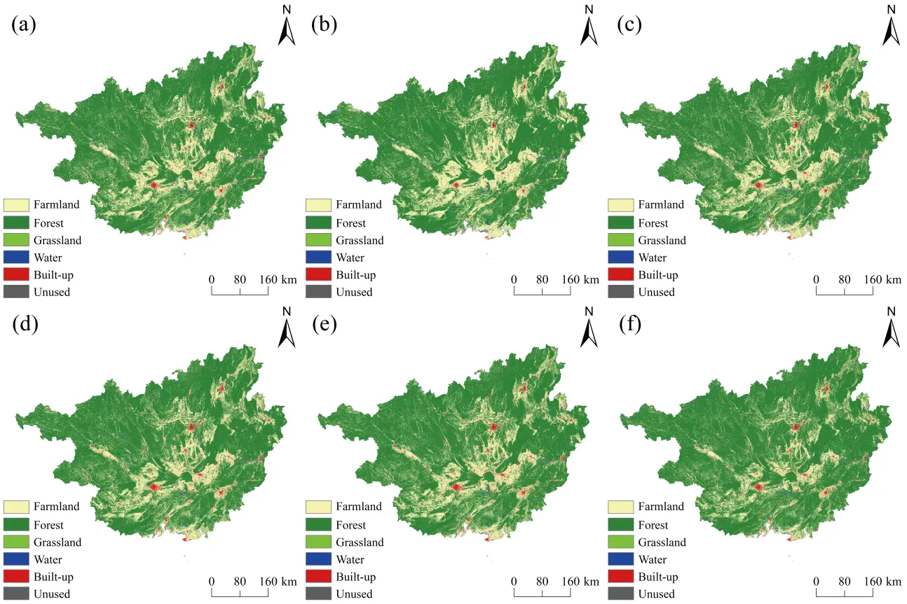
Figure 3. Spatiotemporal evolution of land use in Guangxi. Notes: (a) 2000; (b) 2010; (c) 2020; (d) 2030 under the ND scenario; (e) 2030 under the ED scenario; (f) 2030 under the EP scenario.
3.1.3. Land Use Transition Analysis
As shown in Figure 4, from 2000 to 2010, significant land use transitions occurred in Guangxi. Farmland was mainly converted to forest land and construction land, with transition areas of 6128.56 km2 and 563.00 km2, respectively. During the same period, forest land expansion was primarily driven by the conversion from farmland (7810.19 km2) and grassland (93.19 km2), totaling approximately 7903.38 km2. Between 2010 and 2020, the transition patterns were similar, with farmland again predominantly converted to forest land (9500.13 km2) and construction land (846.00 km2). Compared to the previous decade, the amount of farmland lost to both forest and construction land increased, likely due to ongoing agricultural restructuring, urban expansion, and tourism development [49].
Scenario-based projections for 2030 reveal different transition dynamics: under the ND scenario, farmland is primarily converted to construction land (671.38 km2) and forest land (374.19 km2). Construction land expansion mainly originates from farmland (671.38 km2) and a small portion from forest land (16.19 km2). In the ED scenario, farmland transitions to forest land (335.38 km2) and to construction land (850.63 km2), totaling 1186.01 km2 of conversion. Construction land increases by 1071.88 km2, mostly sourced from farmland and forest land. Under the EP scenario, farmland is largely restored to forest land (10,135.88 km2), with a smaller portion converted to construction land (394.56 km2). Overall, the ED scenario shows the strongest trend of farmland being converted to construction land, whereas the EP scenario emphasizes ecological restoration, especially farmland to forest transformation. This suggests that ecological protection policies (such as reforestation programs and stricter regulations on ecological land encroachment) can effectively limit the expansion of construction land while supporting the increase in ecological land area [50].
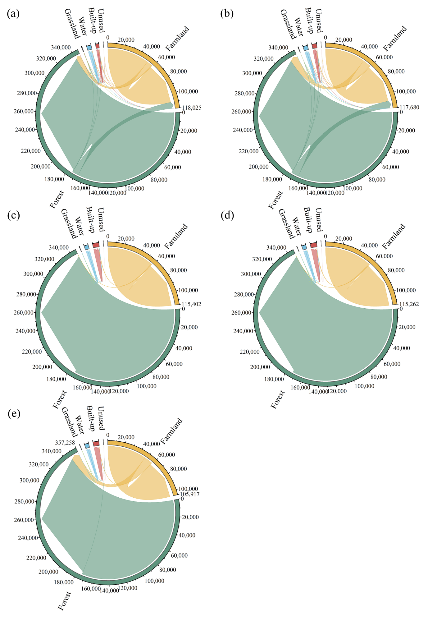
Figure 4. Land use transition map of Guangxi (unit: km2). Notes: (a) 2000–2010; (b) 2010–2020; (c) 2020–2030 ND scenario; (d) 2020–2030 ED scenario; (e) 2020–2030 EP scenario.
3.2. Spatiotemporal Distribution Characteristics of Landscape Ecological Risk
The natural breaks classification method is a statistical technique for categorizing data based on inherent numerical distribution patterns. By automatically identifying statistically significant breakpoints derived from the distribution characteristics of landscape ecological risk, it groups areas with similar risk values, thereby accurately reflecting regional risk conditions [51]. In this study, landscape ecological risk was classified into five levels using the natural breaks method based on the year 2000 data. The same classification criteria were applied to subsequent years for consistency, as detailed in Table 6.
Table 6. Classification of landscape ecological risk levels.
|
Risk Levels |
ERI Value Intervals |
|---|---|
|
Low-risk area |
0.019–0.131 |
|
Medium-low risk area |
0.131–0.135 |
|
Medium risk area |
0.135–0.139 |
|
Medium-high risk area |
0.139–0.148 |
|
High-risk area |
0.148–0.169 |
From 2000 to 2020, the landscape ecological risk in Guangxi was dominated by medium-risk and medium-low-risk zones, with a gradual reduction in high-risk areas (Figure 5, Table 7). Overall, ecological risk showed a trend of steady improvement during this period. In 2000, the low-risk zone covered 108,535.44 km2, accounting for 45.73% of the area, representing the largest category and indicating a relatively stable ecological environment in Guangxi at that time. The medium-low-risk and medium-risk zones occupied 53,532.69 km2 (22.55%) and 29,138.13 km2 (12.28%), respectively, indicating that most of the region experienced relatively low ecological risk. However, the high-medium-risk and high-risk zones accounted for 13.96% and 5.48%, respectively, highlighting some degree of ecological vulnerability. By 2010, the low-risk area increased to 121,245.88 km2 (51.08%), with the medium-low-risk zone also expanding slightly to 53,687.50 km2(22.62%). Meanwhile, the medium-risk zone decreased to 26,785.56 km2 (11.29%), and both the high-medium-risk and high-risk zones shrank to 26,633.56 km2 (11.22%) and 8999.69 km2 (3.79%), respectively. In 2020, the low-risk zone further expanded to 140,336.31 km2 (59.13%), and the medium-low-risk zone increased to 58,376.63 km2 (24.59%). Correspondingly, the medium-risk and high-medium-risk areas continued to decline to 22,925.13 km2 (9.66%) and 13,795.56 km2 (5.81%), respectively, while the high-risk zone significantly dropped to 1918.56 km2 (0.81%). Under the 2030 ND scenario, the low-risk zone area was projected to be 141,548.81 km2(59.64%), similar to 2020, indicating relative ecological stability. The medium-low-risk zone slightly decreased to 57,328.38 km2 (24.15%), while the high-medium-risk and high-risk zones remained low at 13,719.44 km2 (5.78%) and 1910.94 km2 (0.81%), respectively. Under the 2030 ED scenario, the low-risk and medium-low-risk zones were 141,914.19 km2 (59.79%) and 57,033.88 km2 (24.03%), respectively, showing minor changes, whereas the high-medium-risk zone increased slightly to 13,806.81 km2 (5.82%). In contrast, under the 2030 EP scenario, the low-risk zone decreased to 126,011.56 km2 (53.09%), while the medium-low-risk zone increased significantly to 67,602.94 km2 (28.48%), reflecting the positive impact of ecological protection measures on environmental improvement. In summary, the landscape ecological risk in Guangxi exhibited a clear downward trend from 2000–2020, with expanding low-risk and medium-low-risk zones. The EP scenario demonstrated the most effective control over landscape ecological risk, underscoring the beneficial effects of ecological protection policies.
Table 7. Area statistics of ecological risk zones from 2000 to 2030.
|
Risk Levels |
2000 |
2010 |
2020 |
2030 ND |
2030 ED |
2030EP |
||||||
|---|---|---|---|---|---|---|---|---|---|---|---|---|
|
Area (km2) |
(%) |
Area (km2) |
(%) |
Area (km2) |
(%) |
Area (km2) |
(%) |
Area (km2) |
(%) |
Area (km2) |
(%) |
|
|
Low |
108,535.44 |
45.73 |
121,245.88 |
51.08 |
140,336.31 |
59.13 |
141,548.81 |
59.64 |
141,914.19 |
59.79 |
126,011.56 |
53.09 |
|
Medium-low |
53,532.69 |
22.55 |
53,687.50 |
22.62 |
58,376.63 |
24.59 |
57,328.38 |
24.15 |
57,033.88 |
24.03 |
67,602.94 |
28.48 |
|
Medium |
29,138.13 |
12.28 |
26,785.56 |
11.29 |
22,925.13 |
9.66 |
22,844.63 |
9.62 |
22,689.38 |
9.56 |
26,277.44 |
11.07 |
|
Medium-high |
33,136.06 |
13.96 |
26,633.56 |
11.22 |
13,795.56 |
5.81 |
13,719.44 |
5.78 |
13,806.81 |
5.82 |
15,296.06 |
6.44 |
|
High |
13,009.88 |
5.48 |
8999.69 |
3.79 |
1918.56 |
0.81 |
1910.94 |
0.81 |
1907.94 |
0.80 |
2164.19 |
0.91 |
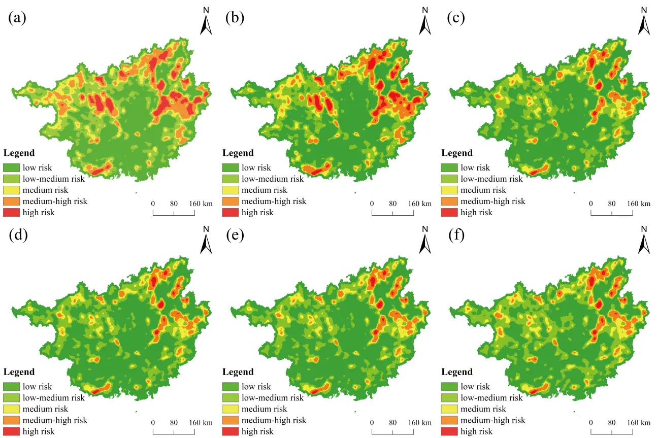
Figure 5. Landscape ecological risk levels in the study area from 2000 to 2030. Notes: (a) 2000, (b) 2010, (c) 2020, (d) 2030 ND scenario, (e) 2030 ED scenario, (f) 2030 EP scenario.
3.3. Analysis of the Spatiotemporal Variation Characteristics of CS
3.3.1. CS Changes from 2000 to 2020
As shown in Table 8, the CS within the study area experienced certain fluctuations between 2000 and 2020. The total CS decreased from 194,131.91 × 104 t in 2000 to 193,091.80 × 104 t in 2020, a reduction of 1040.11 × 104 t. Specifically, CS declined by 555.9 × 10⁴ t during 2000–2010, but partially rebounded with an increase of 478.1 × 10⁴ t from 2010 to 2020. Among different land use types, forest land consistently accounted for the largest share of CS. Although forest CS decreased slightly from 173,110.84 × 104 t in 2000 to 171,972.36 × 104 t in 2020 (a reduction of 1138.48 × 104 t) its proportion only marginally declined by 0.11%. Farmland CS showed relatively minor variation, with an overall decrease of 77.51 × 10⁴ t and a negligible proportion drop of 0.02%. Grassland CS exhibited a more pronounced decline, falling from 99.13 × 10⁴ t in 2000 to 46.27 × 10⁴ t in 2020, a reduction of 52.86 × 10⁴ t, and a 0.03% decrease in its share, indicating a continuous downward trend. Water bodies showed minimal change, with CS in 2020 nearly equal to that in 2000, exhibiting only a slight decrease. In contrast, construction land CS increased significantly, rising from 233.62 × 10⁴ t to 462.26 × 10⁴ t (an increase of 228.64 × 10⁴ t) with its proportion doubling from 0.12% to 0.24%. Unused land maintained the smallest share of CS, with minimal change over the two decades. Overall, despite fluctuations in total CS, the changes across land use types reflect that forest land remains the dominant carbon sink, while CS in farmland and grassland has declined, and that in construction land has grown rapidly.
Table 8. CS of land use in Guangxi at different periods (unit: 104 t).
|
Type |
2000 |
2010 |
2020 |
|||
|---|---|---|---|---|---|---|
|
CS (104 t) |
(%) |
CS (104 t) |
(%) |
CS (104 t) |
(%) |
|
|
Farmland |
20,682.70 |
10.65 |
21,025.36 |
10.90 |
20,605.19 |
10.67 |
|
Forest |
173,110.84 |
89.17 |
171,394.83 |
88.89 |
171,972.36 |
89.06 |
|
Grassland |
99.13 |
0.05 |
69.09 |
0.04 |
46.27 |
0.02 |
|
Water bodies |
5.19 |
0.00 |
5.77 |
0.00 |
5.18 |
0.00 |
|
Construction land |
233.62 |
0.12 |
321.96 |
0.17 |
462.26 |
0.24 |
|
Unused land |
0.43 |
0.00 |
0.20 |
0.00 |
0.53 |
0.00 |
|
Total |
194,131.91 |
100.00 |
192,817.22 |
100.00 |
193,091.80 |
100.00 |
3.3.2. CS Changes Under Different Future Scenarios
According to Table 9, the total CS in the study area in 2020 was 193,091.80 × 104 t. Among land use types, forest land contributed the most, storing 171,972.36 × 104 t, which accounted for approximately 89% of the total. Farmland held 20,605.19 × 104 t, or 10.67%, while other land categories had significantly lower carbon stocks: grassland stored 46.27 × 10⁴ t, water bodies 5.18 × 10⁴ t, construction land 462.26 × 10⁴ t, and unused land just 0.53 × 10⁴ t.
By 2030, CS patterns under different scenarios varied significantly based on projected land use changes. Under the ND scenario, total CS slightly increased to 193,230.20 × 104 t, up by 138.4 × 10⁴ t. Farmland carbon stock rose modestly to 20,234.48 × 104 t, and forest land also increased slightly to 172,353.22 × 104 t. In contrast, grassland CS decreased to 40.67 × 10⁴ t. Notably, construction land CS rose substantially to 596.60 × 10⁴ t, indicating ongoing land development. In the ED scenario, total CS reached 193,167.85 × 104 t (slightly lower than under the ND scenario), with a net decrease of 62.35 × 10⁴ t. Although carbon stock in construction land increased further to 623.12 × 10⁴ t, farmland and grassland CS declined to 20,186.46 × 104 t and 40.33 × 10⁴ t, respectively. Forest land CS remained similar to the ND scenario at 172,312.72 × 104 t, and water bodies held steady at 4.70 × 10⁴ t. This reflects the trade-off between urban expansion and ecosystem carbon capacity. Under the EP scenario, total CS rose significantly to 199,632.00 × 104 t (an increase of 6600.2 × 104 t compared to 2020), highlighting the effectiveness of conservation measures. Forest land CS increased substantially to 182,179.12 × 104 t, representing the greatest gain across all scenarios and confirming the benefits of forest restoration. In contrast, farmland CS dropped significantly to 16,881.20 × 104 t, reflecting the constraints placed on farmland expansion. Grassland CS increased slightly to 43.21 × 10⁴ t—higher than under ND but still below ED levels. Construction land CS decreased to 523.19 × 10⁴ t, while unused land slightly increased to 0.60 × 10⁴ t. In summary, total CS increases under all three scenarios relative to the 2020 baseline. However, the ED scenario exhibits the smallest net gain, largely due to ongoing urbanization. In contrast, the EP scenario shows the largest increase, driven by forest expansion and farmland reduction. The ND scenario reflects relatively stable dynamics with modest carbon stock gains. These results demonstrate that ecological protection policies (such as afforestation, reforestation, and strict land use controls) are highly effective in enhancing forest CS and mitigating losses in other land categories. In comparison, while ED may contribute to construction-related carbon gains, it tends to reduce the overall ecological carbon balance. Therefore, adopting conservation-oriented land use strategies is key to maximizing regional CS potential.
Table 9. CS under different land use scenarios in 2030 (unit: 104 t).
|
Scenario |
Farmland |
Forest |
Grassland |
Water Bodies |
Construction Land |
Unused Land |
Total |
|---|---|---|---|---|---|---|---|
|
2020 |
20,605.19 |
171,972.36 |
46.27 |
5.18 |
462.26 |
0.53 |
193,091.80 |
|
2030 ND |
20,234.48 |
172,353.22 |
40.67 |
4.70 |
596.60 |
0.53 |
193,230.20 |
|
2030 ED |
20,186.46 |
172,312.72 |
40.33 |
4.70 |
623.12 |
0.52 |
193,167.85 |
|
2030 EP |
16,881.20 |
182,179.12 |
43.21 |
4.69 |
523.19 |
0.60 |
199,632.00 |
3.3.3. Spatial Distribution of CS in Guangxi
Figure 6 illustrates the spatial distribution of CS in Guangxi. High CS values are primarily concentrated in the western and southern mountainous regions. These areas are typically characterized by dense forest cover, relatively stable ecological conditions, and strong carbon sequestration capacity. In particular, the southwestern mountainous zones (often under better environmental protection) exhibit significant forest carbon stocks. Forest land dominates CS in these regions due to favorable topography, climate, and biodiversity. Higher elevations combined with rich vegetation promote soil carbon accumulation, resulting in concentrated high carbon zones mostly located in mountainous and hilly terrain.
In contrast, areas with lower CS are mainly found in the eastern, coastal, and rapidly urbanizing parts of Guangxi. The lower carbon stocks in these areas are largely due to urban expansion, agricultural intensification, and land development, which reduce the land’s ability to store carbon. Specifically, in the eastern and coastal zones, ongoing urbanization and industrial growth have converted previously carbon-rich lands into construction and industrial areas, leading to a significant decline in CS. Although CS associated with built up land has increased slightly, the overall carbon stock remains low, reflecting the negative impact of land use change. Additionally, the expansion of agricultural and farmland areas has further contributed to declining CS, particularly in regions where farmland carbon density is relatively low. This trend is especially evident in parts of eastern Guangxi, where the shift from natural or forested land to farmland has led to a notable reduction in total CS.
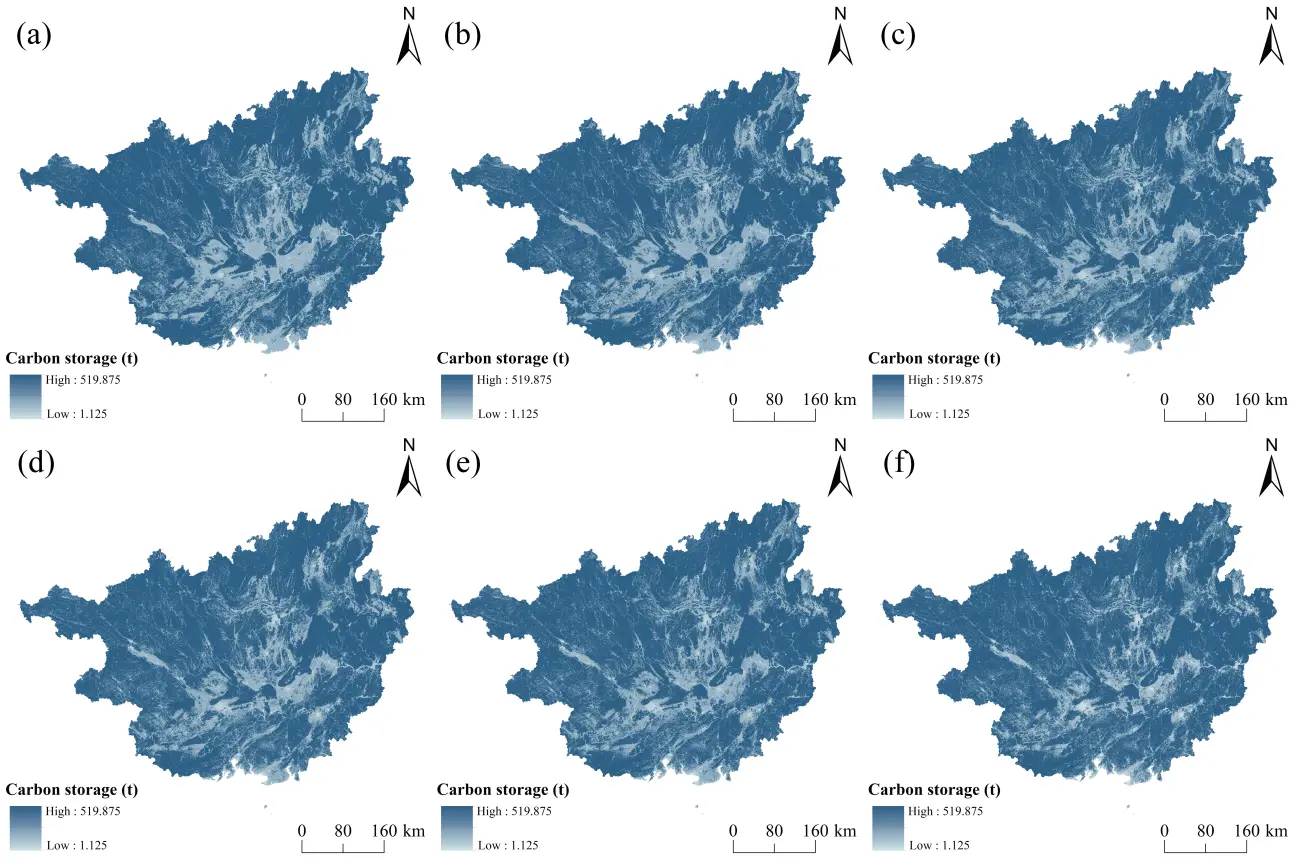
Figure 6. Spatial analysis of CS in Guangxi from 2000 to 2030. Notes: (a) 2000, (b) 2010, (c) 2020, (d) 2030 ND scenario, (e) 2030 ED scenario, (f) 2030 EP scenario.
3.4. Spatial Differentiation of CS in Guangxi
To further elucidate the spatial relationship between land use ecological risk and CS in the study area, both the Global Moran’s I and Local Moran’s I indices were employed. The results (Figure 7) show that from 2000 to 2030, the Global Moran’s I values for CS remained positive, with all p values less than 0.01, indicating a significant positive spatial auto-correlation and notable spatial clustering of CS. From 2000 to 2020, the Global Moran’s I exhibited a downward trend followed by an upward rebound, ultimately increasing over time, suggesting that the overall spatial correlation of CS in the region has strengthened. However, projections for 2030 under different scenarios reveal varying trends in spatial clustering. Under the ND scenario, Global Moran’s I decreases slightly, whereas under the ED scenario, the decline is more pronounced, indicating a weakening spatial clustering effect of CS. In contrast, under the EP scenario, Global Moran’s I increases relative to 2020, suggesting that ecological protection measures enhance the spatial aggregation of CS within the region.
Local spatial autocorrelation analysis was further conducted to characterize the specific clustering patterns and their geographic distribution. As shown in Figure 7, CS clusters in Guangxi are mainly categorized into three types: High-High (H-H), Low-Low (L-L), and High-Low (H-L). H-H clusters are primarily concentrated in the central and western mountainous areas of Guangxi, particularly where forest cover is dense. These areas exhibit high levels of CS, closely associated with the distribution of forest land, which serves as the dominant carbon sink. L-L clusters are mainly found in the southern coastal areas of Guangxi, where rapid urbanization and expansion of construction land have contributed to lower CS values. H-L clusters occur in peri-urban zones and regions with concentrated industrial development. These patterns may result from the outward migration of rural populations due to urbanization, which reduces ecological pressure around rural settlements, allowing for ecological recovery and a corresponding increase in CS.
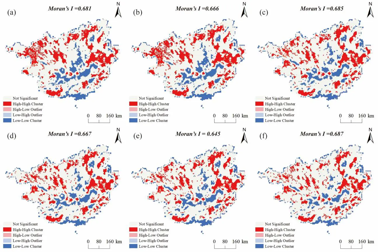
Figure 7. LISA cluster map of CS in Guangxi from 2000 to 2030. Notes: (a) 2000, (b) 2010, (c) 2020, (d) 2030 ND scenario, (e) 2030 ED scenario, (f) 2030 EP scenario.
4. Discussion
4.1. Spatial Relationship Between Ecological Risk and Land Use
The analysis of the landscape ecological risk index reveals a gradual improvement in ecological risk levels in Guangxi from 2000 to 2020, particularly with a noticeable reduction in high-risk areas and expansion of low-risk areas. The landscape ecological risk assessment model effectively demonstrates the impact of various land use types on the ecological environment. The expansion of construction land and the reduction of agricultural land have led to increased ecological risks in some areas—this trend is especially pronounced under the ED scenario. In contrast, under the EP scenario, optimized land use structures have significantly mitigated ecological risks, with a marked rise in low-risk zones. These results highlight the positive impact of ecological conservation policies, showing that strict land protection measures improve environmental quality.
4.2. Relationship Between Ecological Risk and CS
The intricate geographical relationship between CS and ecological danger is revealed by this study. At the macro level, some regions exhibit a coupling pattern of high CS and low ecological risk. These areas are typically located in forested mountainous zones with stable ecosystems and strong carbon sequestration capacities. The high CS in such regions primarily stems from forest land, especially from above ground biomass, below ground biomass, and soil carbon pools. These areas experience less human disturbance, resulting in lower ecological risk. However, in rapidly urbanizing regions, increased CS does not necessarily equate to reduced ecological risk. In some cases, expansion of construction land leads to simultaneous increases in both CS and ecological risk. Specifically, in the eastern coastal and highly urbanized areas, the reduction of forest land and expansion of construction land have led to decreased CS and heightened ecological risk. This underscores the bidirectional impact of land use change on CS and ecological risk. The relationship between the two is influenced by multiple interacting factors, including land use transitions, urbanization, and geographical conditions. Therefore, future carbon sequestration efforts must also prioritize ecological risk management by implementing appropriate ecological protection strategies.
4.3. Drivers of CS Changes Under Different Land Use Scenarios
Land use transition is a key driver of CS changes in Guangxi. The shifts observed between 2000 and 2020 were primarily driven by changes in land use types. According to Table 4, forest land area declined, while construction land expanded from 1571.44 km2 in 2000 to 3111.94 km2 in 2020. As shown in Table 8, forest CS decreased by approximately 1138.48 × 104 t during this period, accounting for the majority of the total reduction. The decline in forest land is likely attributed to the conversion of forests and grasslands to urban land during rapid urbanization.
To better understand the drivers of CS changes, this study employed a Random Forest Classification (RFC) model to quantitatively assess the contributions of different driving factors to land use type changes (Figure 8). The results show that changes in farmland, forest, grassland, water bodies, construction land, and unused land are influenced not only by natural factors such as average temperature and elevation, but also by socioeconomic factors including GDP, transportation accessibility, and population density. For farmland, proximity to transportation infrastructure (e.g., roads, railways) and distance from government centers significantly influence accessibility and development potential. Climatic variables such as mean annual temperature and precipitation also play a key role in determining farmland suitability. Similarly, forest land changes are largely driven by transportation and climate factors, with proximity to infrastructure being especially influential, whereas economic and demographic factors have less impact. Grassland changes are also influenced by transportation and climate, though the magnitude of their influence varies. Water body changes are primarily driven by proximity to transportation and climatic conditions, with minimal influence from GDP and population density. In contrast, construction land is strongly influenced by proximity to major infrastructure such as roads, railways, and government facilities, reflecting the role of government planning and transportation networks. ED and population density also significantly contribute to the expansion of construction land. Unused land, however, is mainly affected by transportation accessibility and climate, with minimal influence from economic or demographic factors. Overall, transportation infrastructure and climatic conditions are the most consistent drivers across land use types, particularly for farmland, forest, grassland, and water bodies, while economic and population factors tend to have more localized and indirect effects.
Under different land use scenarios, CS trends vary significantly. In the ND scenario, CS shows a relatively stable and slight increase, with minor changes in farmland and forest carbon stocks due to improvements in agricultural practices and local land use adjustments. In the ED scenario, rapid expansion of construction land results in a net decrease in total CS. Although CS in construction land increases, this fails to offset the declines in farmland and grassland CS, especially due to the conversion of high-carbon land to lower-carbon urban land, reflecting the negative impact of urbanization. In contrast, the EP scenario shows a significant increase in CS, primarily driven by strict land protection measures such as reforestation, grassland expansion, and constraints on construction land expansion. These efforts promote forest recovery and substantially enhance forest carbon stocks. Overall, the EP scenario not only boosts CS but also strengthens ecological stability in the region, demonstrating the critical role of ecological policies in enhancing carbon sequestration capacity.
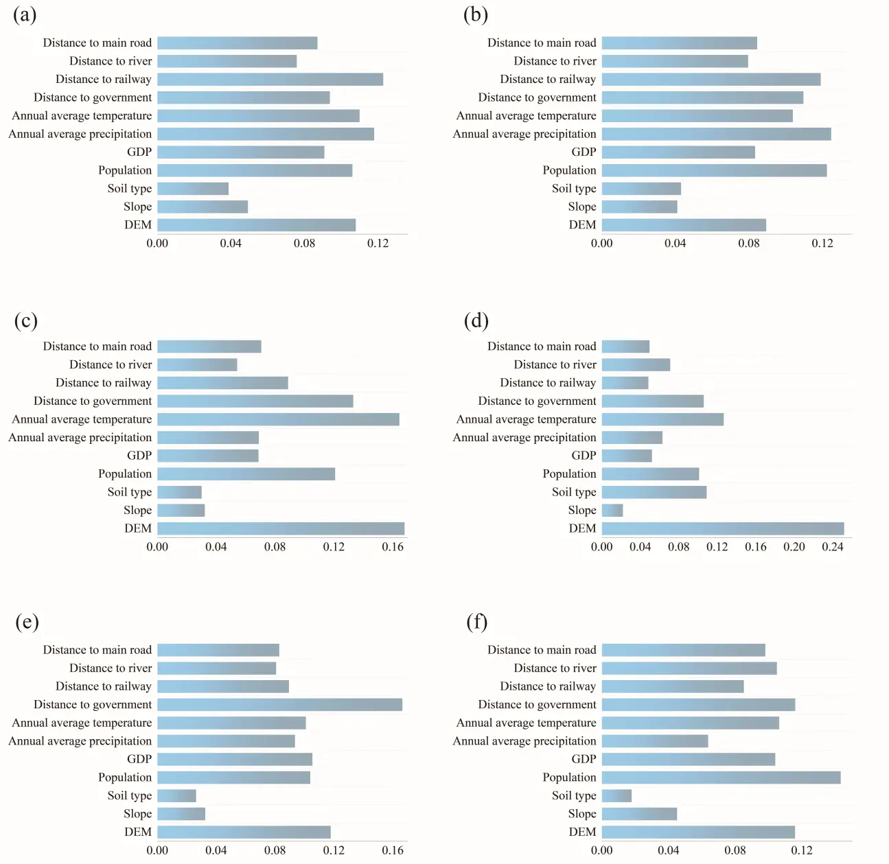
Figure 8. Contribution of different driving factors to CS changes across various land use types. Notes: (a) Farmland, (b) Forest, (c) Grassland, (d) Water, (e) Built-up, (f) Unused.
4.4. Spatial Clustering Characteristics of CS and Ecological Risk
This study employed LISA (Local Indicators of Spatial Association) cluster analysis to explore the spatial distribution characteristics of CS and ecological risk across different regions in Guangxi. High carbon–low risk clusters are mainly concentrated in the mountainous areas of central and western Guangxi. These regions possess high levels of CS and exhibit low ecological risk, largely due to dense forest coverage and the strong carbon sequestration capacity of forest lands. Additionally, these areas maintain relatively stable ecological environments and are less disturbed by human activities. The implementation of forest restoration and protection measures has played a vital role in enhancing CS in these regions. Low carbon–high risk clusters are primarily distributed in coastal and highly urbanized regions, where CS is generally low due to rapid urbanization and the expansion of construction land. As agricultural land is increasingly converted into urban areas, lands that once contributed to carbon sequestration are transformed into construction land with minimal CS capacity. This transformation has led to reduced CS and increased ecological risk in these areas. Consequently, the ecological environments in L-L clusters are more fragile and require urgent ecological restoration and protection efforts. High-low (H-L) clusters are observed in urban–rural fringe zones and some industrially concentrated areas. These regions tend to have relatively high CS but also elevated ecological risk. This pattern is often linked to land use changes driven by local industrial development or urban expansion. In such areas, increases in CS may coincide with rising ecological risks. Thus, optimizing land use structure is essential to simultaneously enhance CS and mitigate ecological risks.
4.5. Recommendations for Optimizing CS and Landscape Ecological Risk
4.5.1. Protection and Enhancement of High Carbon-Low Risk Areas
The high carbon–low risk areas in Guangxi are mainly located in the mountainous regions of the central and western parts of the province. These areas maintain stable ecosystems and high CS. For these zones, strict conservation measures should be enforced to enhance forest restoration and prevent carbon losses caused by inappropriate land development.
4.5.2. Restoration and Protection of Low Carbon-High Risk Areas
Low carbon–high risk areas are primarily found in coastal regions and areas undergoing rapid urbanization. These regions exhibit both low CS and high ecological risk. Priority should be given to implementing ecological restoration initiatives in such zones. Under the guidance of strict and permanent protection policies for prime farmland and ecological land, scientific and comprehensive restoration of farmland and forest areas should be promoted to reduce fragmentation and improve ecological stability [52].
4.6. Limitations of This Study
4.6.1. Model Limitations
Although the PLUS-InVEST model effectively simulates the spatiotemporal evolution of land use and CS, its accuracy and adaptability may be affected by data quality and input parameters. At the regional scale, the predictive outcomes may also be influenced by uncertainties related to spatial resolution and data sources. Therefore, when applied at higher resolutions or finer spatial scales, the model may introduce certain degrees of error.
4.6.2. Scenario Assumption Limitations
This study considers three scenarios: ND, ED, and EP. However, these scenarios are relatively simplified and may not fully account for the complex interplay of socio-economic dynamics, climate change, and policy adjustments. Future research should incorporate more comprehensive and integrated scenario frameworks.
4.6.3. Accuracy of CS Estimations
CS estimations in this study are based on existing carbon density data and the InVEST model. However, the accuracy and applicability of such data can vary across regions. Specifically, different land use types may exhibit distinct carbon density characteristics, requiring more localized and detailed data. The current dataset may not fully capture all intraregional variations. Future work should incorporate more advanced simulation techniques and refined parameters to enhance model accuracy and robustness.
4.6.4. Interpretation and Limitations of the ERI
The ERI used in this study summarizes structural risk inferred from land-use composition and spatial configuration. It is informative for identifying landscape patterns in karst regions that are more likely to be vulnerable; however, it does not directly represent functional ecosystem processes or overall ecosystem condition (e.g., soil erosion, water quality, biodiversity). Accordingly, the scenario comparisons should be read as relative differences in configuration-based risk. In practice, ERI outputs are best used as a screening layer to guide follow-up assessment, and should be considered alongside independent process indicators or field observations.
5. Conclusions
This study applied a coupled PLUS-InVEST model and three land use scenarios to analyze land use changes, CS dynamics, and landscape ecological risk in the ecologically fragile karst region of Guangxi. The results reveal spatiotemporal trends from 2000 to 2020 and responses under different development pathways projected for 2030. The main conclusions are as follows:
- (1)
-
Coupled dynamics of land use, CS, and ecological risk. From 2000 to 2020, farmland in Guangxi declined while construction land expanded rapidly, particularly in urban areas, accompanied by decreases in forest and grassland. This shift, driven by urbanization and farmland conversion, has fragmented CS patterns and increased ecological risk, especially in urban fringes and agricultural zones. The pattern highlights how fragile karst soils limit vegetation recovery and carbon sequestration, while land use transitions reflect development-oriented priorities.
- (2)
-
Scenario-based effects and planning implications. Different land use scenarios lead to distinct spatial responses. The ND scenario continues historical trends with a moderate balance between carbon sinks and ecological risks. The ED scenario increases construction land, reduces overall CS, and raises risk. The ecological conservation scenario, through reforestation and development restrictions, enhances carbon sequestration and reduces ecological risk. Scenario simulations demonstrate that land use structure strongly influences landscape connectivity and carbon sink distribution. These insights support spatial planning tools such as zoning for ecological redlines, risk control zones and differentiated land management, helping align carbon targets with sustainable development.
- (3)
-
Spatial differentiation and regional strategies. High carbon-low risk clusters are mainly found in Guangxi’s central and western mountainous areas, while low carbon-high risk clusters occur in southern coastal and rapidly urbanizing regions. Accordingly, strict protection should be prioritized in high carbon-low risk clusters zones, focusing on forest conservation and ecological regulation. Low carbon-high risk zones should emphasize ecological restoration and green infrastructure. Scenario-driven analysis can guide industrial layout and land structure optimization, providing quantitative support for achieving carbon neutrality and regional sustainability.
Statement of the Use of Generative AI and AI-Assisted Technologies in the Writing Process
During the preparation of this manuscript, the authors used AI tools solely for language polishing and grammar checking. The AI tool was not used for data analysis, model development, result interpretation, or drawing conclusions. After using this tool, the author reviewed and edited the content as needed and take full responsibility for the content of the published article.
Author Contributions
H.J.: Writing original draft. F.W.: Supervision, Writing—review & editing. J.J.: Software, Methodology, Data curation. D.L.: Supervision, Writing—review & editing, Project administration. Z.C.: Writing—review & editing. L.X.: Writing—review & editing. Y.J.: Writing—review & editing. Y.X.: Writing—review & editing.
Ethics Statement
Not applicable.
Informed Consent Statement
Not applicable.
Data Availability Statement
The data presented in this study are available within the article. Further inquiries can be directed to the corresponding author.
Funding
This study was funded by the National Natural Science Foundation of China (42461015), the Guangxi science and technology base and talent special project (GuiKeAD23026194), the Open Fund of key Laboratory for Earth Surface Processes, Ministry of Education, Peking University, the Guangxi Normal University 2025 National Natural Science Foundation of China Joint Cultivation Projects (2025PY037), and the Innovation Project of Guangxi Graduate Education (XYCS2025112).
Declaration of Competing Interest
The authors declare that they have no known competing financial interests or personal relationships that could have appeared to influence the work reported in this paper.
References
-
Shi G, Wang Y, Zhang J, Xu J, Chen Y, Chen W, et al. Spatiotemporal Pattern Analysis and Prediction of Carbon Storage Based on Land Use and Cover Change: A Case Study of Jiangsu Coastal Cities in China. Land 2024, 13, 1728. DOI:10.3390/land13111728 [Google Scholar]
-
Lai J, Qi S, Chen J, Guo J, Wu H, Chen Y. Exploring the spatiotemporal variation of carbon storage on Hainan Island and its driving factors: Insights from InVEST, FLUS models, and machine learning. Ecol. Indic. 2025, 172, 113236. DOI:10.1016/j.ecolind.2025.113236 [Google Scholar]
-
Li W, Zhang SH, Lu C. Exploration of China’s net CO2 emissions evolutionary pathways by 2060 in the context of carbon neutrality. Sci. Total Environ. 2022, 831, 154909. DOI:10.1016/j.scitotenv.2022.154909 [Google Scholar]
-
McDonald RI, Chaplin-Kramer R, Mulligan M, Kropf CM, Hülsen S, Welker P, et al. Win-wins or trade-offs? Site and strategy determine carbon and local ecosystem service benefits for protection, restoration, and agroforestry. Front. Environ. Sci. 2024, 12, 1432654. DOI:10.3389/fenvs.2024.1432654 [Google Scholar]
-
Duguma DW, Brueck M, Shumi G, Law E, Benra F, Schultner J, et al. Future ecosystem service provision under land-use change scenarios in southwestern Ethiopia. Ecosyst. People 2024, 20, 2321613. DOI:10.1080/26395916.2024.2321613 [Google Scholar]
-
Xiang S, Wang Y, Deng H, Yang C, Wang Z, Gao M. Response and multi-scenario prediction of carbon storage to land use/cover change in the main urban area of Chongqing, China. Ecol. Indic. 2022, 142, 109205. DOI:10.1016/j.ecolind.2022.109205 [Google Scholar]
-
Feng Y, Zhang W, Yu J, Zhuo R. Exploring nonlinear land use drivers and multi-scenario strategies for ecological impact mitigation: A case study of the Hohhot-Baotou-Ordos area, Inner Mongolia, China. Cities 2025, 162, 105935. DOI:10.1016/j.cities.2025.105935 [Google Scholar]
-
Zafar Z, Zubair M, Zha Y, Mehmood MS, Rehman A, Fahd S, et al. Predictive modeling of regional carbon storage dynamics in response to land use/land cover changes: An InVEST-based analysis. Ecol. Inform. 2024, 82, 102701. DOI:10.1016/j.ecoinf.2024.102701 [Google Scholar]
-
Guo Z, Ferrer JV, Hürlimann M, Medina V, Puig-Polo C, Yin K, et al. Shallow landslide susceptibility assessment under future climate and land cover changes: A case study from southwest China. Geosci. Front. 2023, 14, 101542. DOI:10.1016/j.gsf.2023.101542 [Google Scholar]
-
Kahsay A, Haile M, Gebresamuel G, Mohammed M, Christopher Okolo C. Assessing land use type impacts on soil quality: Application of multivariate statistical and expert opinion-followed indicator screening approaches. Catena 2023, 231, 107351. DOI:10.1016/j.catena.2023.107351 [Google Scholar]
-
Xu QL, Zhu AX, Liu J. Land-use change modeling with cellular automata using land natural evolution unit. Catena 2023, 224, 106998. DOI:10.1016/j.catena.2023.106998 [Google Scholar]
-
Li M, Liang D, Xia J, Song J, Cheng D, Wu J, et al. Evaluation of water conservation function of Danjiang River Basin in Qinling Mountains, China based on InVEST model. J. Environ. Manag. 2021, 286, 112212. DOI:10.1016/j.jenvman.2021.112212 [Google Scholar]
-
Li P, Chen J, Li Y, Wu W. Using the InVEST-PLUS Model to Predict and Analyze the Pattern of Ecosystem Carbon storage in Liaoning Province, China. Remote Sens. 2023, 15, 4050. DOI:10.3390/rs15164050 [Google Scholar]
-
Liu X, Liu Y, Wang Y, Liu Z. Evaluating potential impacts of land use changes on water supply–demand under multiple development scenarios in dryland region. J. Hydrol. 2022, 610, 127811. DOI:10.1016/j.jhydrol.2022.127811 [Google Scholar]
-
Zhong R, Pu L, Xie J, Yao J, Qie L, He G, et al. Carbon storage in typical ecosystems of coastal wetlands in Jiangsu, China: Spatiotemporal patterns and mechanisms. CATENA 2025, 254, 108882. DOI:10.1016/j.catena.2025.108882 [Google Scholar]
-
Wu X, Shen C, Shi L, Wan Y, Ding J, Wen Q. Spatio-temporal evolution characteristics and simulation prediction of carbon storage: A case study in Sanjiangyuan Area, China. Ecol. Inform. 2024, 80, 102485. DOI:10.1016/j.ecoinf.2024.102485 [Google Scholar]
-
Xia FZ, Huang YJ, Dong LK. Comparison of comprehensive benefits of land-use systems under multi- and single-element governance. Land Use Policy 2024, 141, 107164. DOI:10.1016/j.landusepol.2024.107164 [Google Scholar]
-
Zhou R, Lin M, Gong J, Wu Z. Spatiotemporal heterogeneity and influencing mechanism of ecosystem services in the Pearl River Delta from the perspective of LUCC. J. Geogr. Sci. 2019, 29, 831–845. DOI:10.1007/s11442-019-1631-0 [Google Scholar]
-
Bhushal G, Lal P. Scenario-based economic valuation of forest carbon sequestration in Nepal: Implications for REDD+ (2030–2050). Sustainability 2026, 18, 2468. DOI:10.3390/su18052468 [Google Scholar]
-
Eekhout JPC, de Vente J. Global impact of climate change on soil erosion and potential for adaptation through soil conservation. Earth-Sci. Rev. 2022, 226, 103921. DOI:10.1016/j.earscirev.2022.103921 [Google Scholar]
-
Streck C, Minoli S, Roe S, Barry C, Brander M, Chiquier S, et al. Considering durability in carbon dioxide removal strategies for climate change mitigation. Clim. Policy 2026, 26, 493–501. DOI:10.1080/14693062.2025.2501267 [Google Scholar]
-
Mohr JS, Bastit F, Grünig M, Knoke T, Rammer W, Senf C, et al. Rising cost of disturbances for forestry in Europe under climate change. Nat. Clim. Change 2025, 15, 1078–1083. DOI:10.1038/s41558-025-02408-9 [Google Scholar]
-
Senf C, Seidl R. Mapping the forest disturbance regimes of Europe. Nat. Sustain. 2021, 4, 63–70. DOI:10.1038/s41893-020-00609-y [Google Scholar]
-
Bhavsar A, Hingar D, Ostwal S, Thakkar I, Jadeja S, Shah M. The current scope and stand of carbon capture storage and utilization—A comprehensive review. Case Stud. Chem. Environ. Eng. 2023, 8, 100368. DOI:10.1016/j.cscee.2023.100368 [Google Scholar]
-
Gidden MJ, Joshi S, Armitage JJ, Christ AB, Boettcher M, Brutschin E, et al. A prudent planetary limit for geologic carbon storage. Nature 2025, 645, 124–132. DOI:10.1038/s41586-025-09423-y [Google Scholar]
-
Bai T, Xu D, Bi S, Zhu K, Dávid LD. Impact of green fiscal policy on the collaborative reduction of pollution and carbon emissions: Evidence from energy saving and emission reduction policy in China. Oeconomia Copernic. 2024, 15, 1263–1302. DOI:10.24136/oc.3159 [Google Scholar]
-
Chen DK, Shi LY. The Landscape Ecological Risk Assessment and Prediction for Xiong’an New Area Based on Land Use Change. Ecol. Econ. 2021, 37, 224–229. (In Chinese). Available online: https://kns.cnki.net/kcms2/article/abstract?v=RTWLtMhoy7STQgPYl8N0ZhorTczOg5hARth9KO8CDb_qtvW_saA-Uj8Vt9nfHvH_fNgDCJkmCPPpH8l333X5QxkVm_ZgmluBCiZ2VDNwr_9e1dyysxfpuYEPVeZgqAM5q-32p2HFJaqDPI0pEZdG9CDCeJFO0A35uL0BgmooL8g7Ooc5czxRTQ==&uniplatform=NZKPT&language=CHS (accessed on 18 July 2025).
-
Li S, Tu B, Zhang Z, Wang L, Zhang Z, Che X, et al. Exploring new methods for assessing landscape ecological risk in key basin. J. Clean. Prod. 2024, 461, 142633. DOI:10.1016/j.jclepro.2024.142633 [Google Scholar]
-
Zheng L, Wang Y, Li JF. Quantifying the spatial impact of landscape fragmentation on habitat quality: A multi-temporal dimensional comparison between the Yangtze River Economic Belt and Yellow River Basin of China. Land Use Policy 2023, 125, 106463. DOI:10.1016/j.landusepol.2022.106463 [Google Scholar]
-
Zou Y, Rao Y, Luo F, Yi C, Du P, Liu H, et al. Evolution of rural settlements and its influencing mechanism in the farming-pastoral ecotone of Inner Mongolia from a production-living-ecology perspective. Habitat Int. 2024, 151, 103137. DOI:10.1016/j.habitatint.2024.103137 [Google Scholar]
-
Li WJ, Kang JW, Wang Y. Integrating ecosystem services supply-demand balance into landscape ecological risk and its driving forces assessment in Southwest China. J. Clean. Prod. 2024, 475, 143671. DOI:10.1016/j.jclepro.2024.143671 [Google Scholar]
-
Qian Y, Dong Z, Yan Y, Tang L. Ecological risk assessment models for simulating impacts of land use and landscape pattern on ecosystem services. Sci. Total Environ. 2022, 833, 155218. DOI:10.1016/j.scitotenv.2022.155218 [Google Scholar]
-
Zhang W, Chang WJ, Zhu ZC, Hui Z. Landscape ecological risk assessment of Chinese coastal cities based on land use change. Appl. Geogr. 2020, 117, 102174. DOI:10.1016/j.apgeog.2020.102174 [Google Scholar]
-
Ager AA, Evers CR, Day MA, Alcasena FJ, Houtman R. Planning for future fire: Scenario analysis of an accelerated fuel reduction plan for the western United States. Landsc. Urban Plan. 2021, 215, 104212. DOI:10.1016/j.landurbplan.2021.104212 [Google Scholar]
-
Cortinovis C, Geneletti D. Ecosystem services in urban plans: What is there, and what is still needed for better decisions. Land Use Policy 2018, 70, 298–312. DOI:10.1016/j.landusepol.2017.10.017 [Google Scholar]
-
Neidermeier AN, West TAP, Verburg PH. Navigating trade-offs in carbon storage, biodiversity, and wildfire risk in European landscape management. Ecosyst. Serv. 2025, 74, 101751. DOI:10.1016/j.ecoser.2025.101751 [Google Scholar]
-
Yang J, Huang X. The 30 m annual land cover datasets and its dynamics in China from 1985 to 2023. Earth Syst. Sci. Data 2024, 13, 3907–3925. DOI:10.5194/essd-13-3907-2021 [Google Scholar]
-
Basu T, Das A. Urbanization induced changes in land use dynamics and its nexus to ecosystem service values: A spatiotemporal investigation to promote sustainable urban growth. Land Use Policy 2024, 144, 107239. DOI:10.1016/j.landusepol.2024.107239 [Google Scholar]
-
Gao L, Tao F, Liu R, Wang Z, Leng H, Zhou T. Multi-scenario simulation and ecological risk analysis of land use based on the PLUS model: A case study of Nanjing. Sustain. Cities Soc. 2022, 85, 104055. DOI:10.1016/j.scs.2022.104055 [Google Scholar]
-
Wang J, Wang JM, Zhang JN. Optimization of landscape ecological risk assessment method and ecological management zoning considering resilience. J. Environ. Manag. 2025, 376, 124586. DOI:10.1016/j.jenvman.2025.124586 [Google Scholar]
-
Kurnia AA, Rustiadi E, Fauzi A, Pravitasari AE, Saizen I, Ženka J. Understanding Industrial Land Development on Rural-Urban Land Transformation of Jakarta Megacity’s Outer Suburb. Land 2022, 11, 670. DOI:10.3390/land11050670 [Google Scholar]
-
Zhou X, Ji G, Wang F, Ji X. Identification and simulation of ecological zoning in the Yangtze River Delta (YRD) urban agglomeration based on Ecological Service Value (ESV)–Landscape Ecological Risk (LER). J. Clean. Prod. 2025, 516, 145778. DOI:10.1016/j.jclepro.2025.145778 [Google Scholar]
-
Zhang S, Zhong Q, Cheng D, Xu C, Chang Y, Lin Y, et al. Landscape ecological risk projection based on the PLUS model under the localized shared socioeconomic pathways in the Fujian Delta region. Ecol. Indic. 2022, 136, 108642. DOI:10.1016/j.ecolind.2022.108642 [Google Scholar]
-
Yang Y, Yang M, Zhao B, Lu Z, Sun X, Zhang Z. Spatially explicit carbon emissions from land use change: Dynamics and scenario simulation in the Beijing-Tianjin-Hebei urban agglomeration. Land Use Policy 2025, 150, 107473. DOI:10.1016/j.landusepol.2025.107473 [Google Scholar]
-
Tian L, Tao Y, Fu W, Li T, Ren F, Li M. Dynamic simulation of land use/cover change and assessment of forest ecosystem carbon storage under climate change scenarios in Guangdong Province, China. Remote Sens. 2022, 14, 2330. DOI:10.3390/rs14102330 [Google Scholar]
-
Deng G, Jiang H, Zhu S, Wen Y, He C, Wang X, et al. Projecting the response of ecological risk to land use/land cover change in ecologically fragile regions. Sci. Total Environ. 2024, 914, 169908. DOI:10.1016/j.scitotenv.2024.169908 [Google Scholar]
-
Jiang W, Deng Y, Tang Z, Lei X, Chen Z. Modelling the potential impacts of urban ecosystem changes on carbon storage under different scenarios by linking the CLUE-S and the InVEST models. Ecol. Model. 2017, 345, 30–40. DOI:10.1016/j.ecolmodel.2016.12.002 [Google Scholar]
-
Liu F, Yang L, Wang S. Spatial and temporal evolution and correlation analysis of landscape ecological risks and ecosystem service values in the Jinsha River Basin. J. Resour. Ecol. 2023, 14, 914–927. DOI:10.5814/j.issn.1674-764x.2023.05.003 [Google Scholar]
-
Jing J, Wei F, Jiang H, Chen Z, Lv S, Li T, et al. Prediction of Land Use Change and Carbon Storage in Lijiang River Basin Based on InVEST-PLUS Model and SSP-RCP Scenario. Land 2025, 14, 460. DOI:10.3390/land14030460 [Google Scholar]
-
He Y, Ma J, Zhang C, Yang H. Spatio-Temporal Evolution and Prediction of Carbon Storage in Guilin Based on FLUS and InVEST Models. Remote Sens. 2023, 15, 1445. DOI:10.3390/rs15051445 [Google Scholar]
-
Chen J, Yang ST, Li HW, Zhang B, Lv JR. Research on geographical environment unit division based on the method of natural breaks (Jenks). Int. Arch. Photogramm. Remote Sens. Spat. Inf. Sci. 2013, 40, 47–50. DOI:10.5194/isprsarchives-XL-4-W3-47-2013 [Google Scholar]
-
Peng Y, Cheng W, Xu X, Song H. Analysis and prediction of the spatiotemporal characteristics of land-use ecological risk and carbon storage in Wuhan metropolitan area. Ecol. Indic. 2024, 158, 11143. DOI:10.1016/j.ecolind.2023.111432 [Google Scholar]