Cost-Aware UAV Photogrammetric Mission Design: Experimental Trade-Offs Between Overlap, Geometry, and Mapping Quality

Cost-Aware UAV Photogrammetric Mission Design: Experimental Trade-Offs Between Overlap, Geometry, and Mapping Quality

Received: 22 January 2026 Revised: 05 February 2026 Accepted: 27 February 2026 Published: 11 March 2026

© 2026 The authors. This is an open access article under the Creative Commons Attribution 4.0 International License (https://creativecommons.org/licenses/by/4.0/).
Graphical Abstract
1. Introduction
1.1. UAV Photogrammetry and 3D City Modeling
Unmanned Aerial Vehicle (UAV) photogrammetry has become a key technology for high-resolution 3D city modeling due to its flexibility, high spatial detail, and relatively low deployment cost [1]. Modern UAV pipelines typically rely on structure-from-motion (SfM) and bundle adjustment for image orientation, followed by multi-view stereo (MVS) for dense reconstruction. While these methods are highly effective for many mapping tasks, urban environments remain challenging due to strong depth discontinuities, repetitive textures, façade occlusions, and narrow street canyons that restrict visibility and weaken ray-intersection geometry [2].
To mitigate these effects, practitioners often adopt conservative acquisition designs—e.g., high overlap, cross-flight patterns, oblique imagery, and/or multi-altitude flights—to increase redundancy and angular diversity. However, these measures substantially increase flight duration, image volume, and processing effort, thereby raising operational and computational costs. Importantly, higher redundancy alone does not guarantee stronger geometry: if viewing directions remain weakly diversified, self-calibration and object-space error propagation may remain unfavorable despite low residuals in the adjustment. Consequently, the core technical question for practical urban UAV mapping is not whether high-overlap networks work (they do), but how to reduce acquisition and processing load while preserving sufficient geometric robustness and product-level mapping quality.
For autonomous and semi-autonomous UAV systems, this trade-off is not merely operational but algorithmic: mission planners must decide acquisition parameters under resource constraints (time/energy/compute) while satisfying task requirements. Recent surveys have highlighted a transition from heuristic, overlap-driven planning toward optimization-based, autonomy-aware decision frameworks that explicitly combine mapping objectives with resource constraints and feasibility considerations [3,4].
1.2. Related Work on Image Acquisition Parameters for 3D City Modeling
Prior research on UAV acquisition design for 3D reconstruction can be broadly grouped into three lines of work. First, several studies have examined how overlap percentages and flight-line patterns influence orientation stability, completeness, and accuracy. The common finding is that higher overlap generally increases tie-point redundancy and reconstruction robustness, but accuracy gains may saturate beyond moderate overlap levels, whereas processing time and data volume continue to grow rapidly [2,5]. These results suggest that conservative “one-size-fits-all” overlap rules may be inefficient when cost and turnaround time matter.
Second, a substantial body of work has emphasized that viewing-geometry diversification—rather than redundancy alone—is critical in complex scenes. In particular, oblique imagery and hybrid nadir–oblique designs can increase visibility of façades and improve urban completeness and geometric stability compared with nadir-only acquisitions [6]. Likewise, camera orientation and flight design choices (including oblique setups and flight-direction changes) have been shown to affect the quality of the derived 3D products, especially in settings with occlusions and complex geometry [7]. Multi-altitude acquisition has also been reported as an effective mechanism for strengthening intersection geometry and improving 3D reconstruction performance in urban environments [8].
Third, mission-planning research in robotics and autonomous UAV systems has increasingly focused on optimization-based planning that links task objectives to constraints and resources (e.g., time, energy, and risk) [3,4]. Nevertheless, much of this literature is generic with respect to photogrammetric quality indicators, and often lacks experimentally validated, product-specific rules that map acquisition parameters to cost–quality outcomes in real mapping workflows.
Research gap (problem-oriented). Despite the above advances, experimentally controlled studies that jointly evaluate (i) operational cost proxies, (ii) processing effort proxies, (iii) geometric strengthening mechanisms (cross-flight, oblique, and multi-altitude), and (iv) product-dependent mapping quality within a single, consistent experimental framework remain limited for urban blocks at cartographic accuracies. In particular, the literature rarely provides integrated, decision-ready guidance on when overlap reduction is acceptable, how it should be geometrically compensated, and how these trade-offs change with the target product (e.g., vector mapping, orthomosaics, or dense 3D meshes). This paper addresses this gap through a controlled and comparable evaluation of multiple acquisition strategies under realistic urban conditions, explicitly positioning the results for cost-aware and autonomy-aware mission planning.
Despite these contributions, most existing studies address acquisition overlap, viewing geometry, accuracy, or mission efficiency in isolation, or consider only subsets of these factors. Comprehensive experimental studies that simultaneously combine operational cost proxies, processing effort, geometric configuration, and product-dependent quality assessment within a unified and controlled evaluation framework remain scarce, particularly for urban UAV photogrammetry.
1.3. Terminologies
To avoid ambiguity, we use the following terminology consistently throughout the paper. Overlap-driven planning refers to heuristic designs that primarily prescribe conservative endlap/sidelap values. Accuracy-driven planning prioritizes maximizing geometric accuracy and completeness without explicitly modeling operational or computational burden. Cost-aware planning aims to minimize operational and processing effort subject to achieving acceptable mapping quality. Autonomy-aware planning refers to optimization-based decision-making frameworks that explicitly consider task objectives, constraints, and feasibility, and may adapt decisions online. Finally, product-dependent means that “acceptable quality” (and thus the preferred acquisition design) depends on the target deliverable (MAP, OIM, or 3DMesh).
1.4. Objectives and Contributions
The objective of this study is to develop and experimentally validate Accuracy-driven, cost-aware, and product-dependent UAV photogrammetric mission designs for large-scale urban mapping, and to provide quantitative evidence that can be embedded into autonomy-aware mission planners. The main contributions are:
-
-
An integrated and experimentally controlled evaluation framework that simultaneously links operational flight cost, processing effort, geometric configuration, and product-dependent mapping quality, enabling direct comparison of alternative UAV acquisition strategies under realistic urban conditions.
-
-
A controlled experimental framework for evaluating integrated cost–quality trade-offs in UAV photogrammetric network design using consistent processing and independent checkpoints.
-
-
A comparative assessment of five acquisition strategies that decouple redundancy reduction from geometric strengthening (overlap reallocation, cross-flight compensation, partial high-overlap calibration, multi-altitude acquisition, and oblique cross-flight integration).
-
-
Product-dependent mission-planning guidelines for MAP, OIM, and dense 3D reconstruction, expressed in a form suitable for rule-based and Pareto-driven planning under resource constraints.
-
-
Practical recommendations that support efficient autonomous and semi-autonomous UAV mapping workflows by connecting flight-parameter choices to measurable cost and mapping-quality outcomes.
Unlike previous overlap-centric studies, this work provides a unified experimental Pareto framework linking overlap, geometry, cost proxies, and product-specific mapping objectives across 98 controlled configurations.
2. Conceptual Framework for Cost-Aware Photogrammetric Network Design
2.1. Cost Drivers and Relative Cost Proxies
In UAV photogrammetry, mission effort is dominated by two coupled components: operational effort associated with data acquisition (e.g., flight time and energy consumption), and processing effort associated with reconstruction (e.g., image matching, bundle adjustment, and dense reconstruction). The variables that primarily control these efforts are referred to here as cost drivers. For a fixed ground sampling distance (GSD) and camera frame rate, overlap parameters strongly influence both major cost drivers: (i) the number of flight lines and drone flying speed (hence flight duration), and (ii) the total number of acquired images (hence processing load in structure from motion and multi-view stereo steps). In particular, lateral overlap (sidelap) directly determines the required number of strips and therefore strongly affects acquisition effort, while total image count acts as a primary scaling variable governing computational effort in both SfM and MVS pipelines.
From a computational perspective, image count plays a dominant role in determining processing effort in both structure-from-motion (SfM) and multi-view stereo (MVS) pipelines. In feature-based SfM, pairwise image matching exhibits approximately quadratic scaling in the worst case, O(N2), where N is the number of images, because potential image pairs increase combinatorially. In practical large-scale UAV blocks, graph-based image connectivity and preselection reduce full quadratic matching; however, the effective computational burden still increases super-linearly with N due to feature extraction, correspondence verification, and global optimization steps. Although practical implementations reduce this through image connectivity graphs and preselection strategies, the computational burden remains strongly dependent on the image count. Bundle adjustment further scales with the number of images, tie points, and observations, typically exhibiting super-linear behavior as image redundancy increases.
In dense MVS reconstruction, per-image depth estimation and cross-view consistency checks also scale with the number of images and image resolution, making image count a primary driver of memory consumption and processing time. Similar scaling behavior has been analytically modeled in other image-based processing frameworks, including hybrid CNN–Transformer architectures operating on image datasets, where computational complexity increases rapidly with input image volume [9].
Consequently, even when geometric strengthening strategies improve reconstruction robustness, processing effort remains fundamentally linked to the total number of images, justifying the use of image count (or the normalized processing time derived from it) as a dominant predictor of processing cost in this study.
Because absolute monetary cost depends on platform-, operator-, and hardware-specific factors, this study expresses operational and processing effort using relative cost proxies to enable fair comparison between alternative network designs. These proxies are normalized with respect to a high-overlap reference configuration used as a baseline.
From a decision-theoretic perspective, the normalized cost formulation can be viewed as a dimensionless surrogate objective function within a constrained multi-objective optimization framework, where strip redundancy and image volume act as dominant cost variables, and geometric strengthening strategies (e.g., cross-flight, oblique, multi-altitude acquisition) serve as compensatory design mechanisms.
The exact definitions of the flight and processing cost indices, along with their normalization, are provided in Section 3.4.
2.2. Geometric Strength, Redundancy, and Error Propagation
The spatial configuration of image rays governs the geometric reliability of a photogrammetric network, their intersection angles, and the distribution of redundancy within the bundle adjustment [10,11]. Although high overlap increases observation count, it does not necessarily increase geometric strength if ray directions remain weakly diversified. In such cases, networks may exhibit low residuals while still suffering from unfavorable error propagation and inflated object-space uncertainty.
From a cost-aware perspective, reducing overlaps decreases redundancy and degrees of freedom and can therefore weaken stability unless compensated by improved geometry. Geometric strengthening strategies—such as cross-flight acquisition, oblique imagery, and multi-altitude views—improve ray-intersection diversity and increase information content per observation, enabling comparable robustness with fewer images. Consequently, cost-efficient designs should not be interpreted as “overlap reduction alone”, but rather as redundancy reduction coupled with deliberate geometric strengthening, consistent with classical formulations of aerial triangulation and bundle adjustment [12,13].
2.3. Cost–Quality Trade-Off as a Multi-Objective Design Problem
Network design for UAV photogrammetry can be viewed as a multi-objective decision problem [14] in which mapping quality (accuracy and reconstruction robustness) must be balanced against operational and processing effort. Reducing cost drivers (e.g., image count and strip count) typically reduces redundancy, which may degrade stability unless geometric strength is improved through network reconfiguration (e.g., cross-flight, oblique, or multi-altitude acquisition). This framing motivates the evaluation strategy used in this paper: rather than assuming that maximum overlap is optimal, alternative configurations are assessed in a cost–quality space to identify efficient solutions that achieve acceptable quality at substantially reduced relative cost. The Pareto-style interpretation of these trade-offs is used as an analysis tool in the Results section to support product-dependent recommendations.
3. Methodology
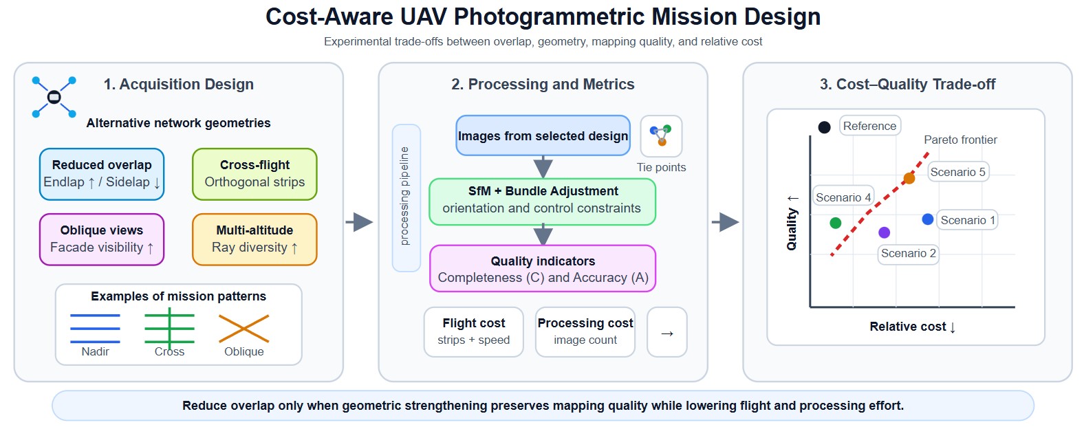
This section describes the experimental methodology used to evaluate cost-aware UAV photogrammetric network designs. The workflow (cf. Figure 1) is structured to systematically isolate the effects of image overlap and network geometry on operational, processing, and overall costs, as well as accuracy and completeness. A high-overlap reference configuration is first established as a benchmark, after which multiple cost-reduction strategies are implemented through controlled variations in lateral overlap, viewing geometry, and flight altitude [13,15]. Each resulting network configuration is processed using an identical photogrammetric pipeline and evaluated using normalized cost and quality indicators, enabling a consistent and objective comparison across scenarios.
%22%2F%3E%3Crect%20x%3D%22140%22%20y%3D%22220%22%20width%3D%22920%22%20height%3D%22140%22%20stroke%3D%22%23111111%22%20stroke-width%3D%222%22%20fill%3D%22%23FFFFFF%22%2F%3E%3Ctext%20fill%3D%22%23111111%22%20font-family%3D%22Arial%2CHelvetica%2CArial%22%20font-weight%3D%22700%22%20font-size%3D%2222%22%20text-anchor%3D%22middle%22%20x%3D%22600%22%20y%3D%22265%22%3EReference%20mission%20design%3C%2Ftext%3E%3Ctext%20fill%3D%22%23111111%22%20font-family%3D%22Arial%2CHelvetica%2CArial%22%20font-size%3D%2220%22%20text-anchor%3D%22middle%22%20x%3D%22600%22%20y%3D%22300%22%3EHigh-overlap%20baseline%20(e.g.%2C%2080%E2%80%9380)%20with%20nadir%20and%20oblique%20imagery%3C%2Ftext%3E%3Ctext%20fill%3D%22%23111111%22%20font-family%3D%22Arial%2CHelvetica%2CArial%22%20font-size%3D%2218%22%20text-anchor%3D%22middle%22%20x%3D%22600%22%20y%3D%22330%22%3ECross-flight%20in%20both%20directions%20(along-%20and%20across-track)%3C%2Ftext%3E%3Cline%20x1%3D%22600%22%20y1%3D%22360%22%20x2%3D%22600%22%20y2%3D%22420%22%20stroke%3D%22%23111111%22%20stroke-width%3D%222.5%22%20fill%3D%22none%22%20marker-end%3D%22url(%23arrow)%22%2F%3E%3Crect%20x%3D%22140%22%20y%3D%22420%22%20width%3D%22920%22%20height%3D%22120%22%20stroke%3D%22%23111111%22%20stroke-width%3D%222%22%20fill%3D%22%23FFFFFF%22%2F%3E%3Ctext%20fill%3D%22%23111111%22%20font-family%3D%22Arial%2CHelvetica%2CArial%22%20font-weight%3D%22700%22%20font-size%3D%2222%22%20text-anchor%3D%22middle%22%20x%3D%22600%22%20y%3D%22465%22%3EPhotogrammetric%20processing%20(common%20pipeline)%3C%2Ftext%3E%3Ctext%20fill%3D%22%23111111%22%20font-family%3D%22Arial%2CHelvetica%2CArial%22%20font-size%3D%2220%22%20text-anchor%3D%22middle%22%20x%3D%22600%22%20y%3D%22500%22%3ETie-point%20extraction%20%E2%86%92%20BA%2FAT%20%E2%86%92%20(optional)%20dense%20reconstruction%3C%2Ftext%3E%3Cline%20x1%3D%22600%22%20y1%3D%22540%22%20x2%3D%22600%22%20y2%3D%22595%22%20stroke%3D%22%23111111%22%20stroke-width%3D%222.5%22%20fill%3D%22none%22%20marker-end%3D%22url(%23arrow)%22%2F%3E%3Crect%20x%3D%22140%22%20y%3D%22595%22%20width%3D%22920%22%20height%3D%22120%22%20stroke%3D%22%23111111%22%20stroke-width%3D%222%22%20fill%3D%22%23FFFFFF%22%2F%3E%3Ctext%20fill%3D%22%23111111%22%20font-family%3D%22Arial%2CHelvetica%2CArial%22%20font-weight%3D%22700%22%20font-size%3D%2222%22%20text-anchor%3D%22middle%22%20x%3D%22600%22%20y%3D%22640%22%3EBaseline%20indicators%3C%2Ftext%3E%3Ctext%20fill%3D%22%23111111%22%20font-family%3D%22Arial%2CHelvetica%2CArial%22%20font-size%3D%2220%22%20text-anchor%3D%22middle%22%20x%3D%22600%22%20y%3D%22675%22%3EBaseline%20cost%20proxies%20%2B%20quality%20(Accuracy%20C%E2%82%90%2C%20Completeness)%3C%2Ftext%3E%3Cline%20x1%3D%22600%22%20y1%3D%22715%22%20x2%3D%22600%22%20y2%3D%22775%22%20stroke%3D%22%23111111%22%20stroke-width%3D%222.5%22%20fill%3D%22none%22%20marker-end%3D%22url(%23arrow)%22%2F%3E%3Crect%20x%3D%22140%22%20y%3D%22775%22%20width%3D%22920%22%20height%3D%22260%22%20stroke%3D%22%23111111%22%20stroke-width%3D%222%22%20stroke-dasharray%3D%2210%208%22%20fill%3D%22%23FFFFFF%22%2F%3E%3Ctext%20fill%3D%22%23111111%22%20font-family%3D%22Arial%2CHelvetica%2CArial%22%20font-weight%3D%22700%22%20font-size%3D%2222%22%20text-anchor%3D%22middle%22%20x%3D%22600%22%20y%3D%22820%22%3EScenario%20definition%20(1%E2%80%935)%3C%2Ftext%3E%3Ctext%20fill%3D%22%23111111%22%20font-family%3D%22Arial%2CHelvetica%2CArial%22%20font-size%3D%2220%22%20text-anchor%3D%22middle%22%20x%3D%22600%22%20y%3D%22855%22%3EControlled%20variations%20in%20overlap%2C%20geometry%2C%20and%20altitude%3C%2Ftext%3E%3Ctext%20fill%3D%22%23111111%22%20font-family%3D%22Arial%2CHelvetica%2CArial%22%20font-size%3D%2218%22%20text-anchor%3D%22middle%22%20x%3D%22600%22%20y%3D%22895%22%3E1)%20Reduced%20sidelap%20%2B%20higher%20endlap%3C%2Ftext%3E%3Ctext%20fill%3D%22%23111111%22%20font-family%3D%22Arial%2CHelvetica%2CArial%22%20font-size%3D%2218%22%20text-anchor%3D%22middle%22%20x%3D%22600%22%20y%3D%22925%22%3E2)%20Cross-flight%20compensation%3C%2Ftext%3E%3Ctext%20fill%3D%22%23111111%22%20font-family%3D%22Arial%2CHelvetica%2CArial%22%20font-size%3D%2218%22%20text-anchor%3D%22middle%22%20x%3D%22600%22%20y%3D%22955%22%3E3)%20Partial%20high-overlap%20calibration%3C%2Ftext%3E%3Ctext%20fill%3D%22%23111111%22%20font-family%3D%22Arial%2CHelvetica%2CArial%22%20font-size%3D%2218%22%20text-anchor%3D%22middle%22%20x%3D%22600%22%20y%3D%22985%22%3E4)%20Multi-altitude%20acquisition%3C%2Ftext%3E%3Ctext%20fill%3D%22%23111111%22%20font-family%3D%22Arial%2CHelvetica%2CArial%22%20font-size%3D%2218%22%20text-anchor%3D%22middle%22%20x%3D%22600%22%20y%3D%221015%22%3E5)%20Oblique%20cross-flight%20integration%3C%2Ftext%3E%3Cline%20x1%3D%22600%22%20y1%3D%221035%22%20x2%3D%22600%22%20y2%3D%221085%22%20stroke%3D%22%23111111%22%20stroke-width%3D%222.5%22%20fill%3D%22none%22%20marker-end%3D%22url(%23arrow)%22%2F%3E%3Crect%20x%3D%22140%22%20y%3D%221085%22%20width%3D%22920%22%20height%3D%22120%22%20stroke%3D%22%23111111%22%20stroke-width%3D%222%22%20fill%3D%22%23FFFFFF%22%2F%3E%3Ctext%20fill%3D%22%23111111%22%20font-family%3D%22Arial%2CHelvetica%2CArial%22%20font-weight%3D%22700%22%20font-size%3D%2222%22%20text-anchor%3D%22middle%22%20x%3D%22600%22%20y%3D%221130%22%3EScenario-based%20network%20construction%3C%2Ftext%3E%3Ctext%20fill%3D%22%23111111%22%20font-family%3D%22Arial%2CHelvetica%2CArial%22%20font-size%3D%2220%22%20text-anchor%3D%22middle%22%20x%3D%22600%22%20y%3D%221165%22%3EBuild%20sub-blocks%20from%20acquired%20datasets%3C%2Ftext%3E%3Cline%20x1%3D%22600%22%20y1%3D%221205%22%20x2%3D%22600%22%20y2%3D%221260%22%20stroke%3D%22%23111111%22%20stroke-width%3D%222.5%22%20fill%3D%22none%22%20marker-end%3D%22url(%23arrow)%22%2F%3E%3Crect%20x%3D%22140%22%20y%3D%221260%22%20width%3D%22920%22%20height%3D%22120%22%20stroke%3D%22%23111111%22%20stroke-width%3D%222%22%20fill%3D%22%23FFFFFF%22%2F%3E%3Ctext%20fill%3D%22%23111111%22%20font-family%3D%22Arial%2CHelvetica%2CArial%22%20font-weight%3D%22700%22%20font-size%3D%2222%22%20text-anchor%3D%22middle%22%20x%3D%22600%22%20y%3D%221305%22%3EPhotogrammetric%20processing%20(same%20pipeline)%3C%2Ftext%3E%3Ctext%20fill%3D%22%23111111%22%20font-family%3D%22Arial%2CHelvetica%2CArial%22%20font-size%3D%2220%22%20text-anchor%3D%22middle%22%20x%3D%22600%22%20y%3D%221340%22%3EIdentical%20settings%20for%20fair%20comparison%3C%2Ftext%3E%3Cline%20x1%3D%22600%22%20y1%3D%221380%22%20x2%3D%22600%22%20y2%3D%221425%22%20stroke%3D%22%23111111%22%20stroke-width%3D%222.5%22%20fill%3D%22none%22%20marker-end%3D%22url(%23arrow)%22%2F%3E%3Crect%20x%3D%22140%22%20y%3D%221425%22%20width%3D%22450%22%20height%3D%22140%22%20stroke%3D%22%23111111%22%20stroke-width%3D%222%22%20fill%3D%22%23FFFFFF%22%2F%3E%3Ctext%20fill%3D%22%23111111%22%20font-family%3D%22Arial%2CHelvetica%2CArial%22%20font-weight%3D%22700%22%20font-size%3D%2222%22%20text-anchor%3D%22middle%22%20x%3D%22365%22%20y%3D%221470%22%3ECost%20evaluation%3C%2Ftext%3E%3Ctext%20fill%3D%22%23111111%22%20font-family%3D%22Arial%2CHelvetica%2CArial%22%20font-size%3D%2220%22%20text-anchor%3D%22middle%22%20x%3D%22365%22%20y%3D%221505%22%3EFlight%20cost%20proxy%3C%2Ftext%3E%3Ctext%20fill%3D%22%23111111%22%20font-family%3D%22Arial%2CHelvetica%2CArial%22%20font-size%3D%2220%22%20text-anchor%3D%22middle%22%20x%3D%22365%22%20y%3D%221535%22%3EProcessing%20cost%20proxy%3C%2Ftext%3E%3Crect%20x%3D%22610%22%20y%3D%221425%22%20width%3D%22450%22%20height%3D%22140%22%20stroke%3D%22%23111111%22%20stroke-width%3D%222%22%20fill%3D%22%23FFFFFF%22%2F%3E%3Ctext%20fill%3D%22%23111111%22%20font-family%3D%22Arial%2CHelvetica%2CArial%22%20font-weight%3D%22700%22%20font-size%3D%2222%22%20text-anchor%3D%22middle%22%20x%3D%22835%22%20y%3D%221470%22%3EQuality%20evaluation%3C%2Ftext%3E%3Ctext%20fill%3D%22%23111111%22%20font-family%3D%22Arial%2CHelvetica%2CArial%22%20font-size%3D%2220%22%20text-anchor%3D%22middle%22%20x%3D%22835%22%20y%3D%221505%22%3EAccuracy%3A%20C%E2%82%90%20(image%20%2B%20ground)%3C%2Ftext%3E%3Ctext%20fill%3D%22%23111111%22%20font-family%3D%22Arial%2CHelvetica%2CArial%22%20font-size%3D%2220%22%20text-anchor%3D%22middle%22%20x%3D%22835%22%20y%3D%221535%22%3ECompleteness%3A%20tie%20points%3C%2Ftext%3E%3Cline%20x1%3D%22365%22%20y1%3D%221565%22%20x2%3D%22365%22%20y2%3D%221625%22%20stroke%3D%22%23111111%22%20stroke-width%3D%222.5%22%20fill%3D%22none%22%20marker-end%3D%22url(%23arrow)%22%2F%3E%3Cline%20x1%3D%22835%22%20y1%3D%221565%22%20x2%3D%22835%22%20y2%3D%221625%22%20stroke%3D%22%23111111%22%20stroke-width%3D%222.5%22%20fill%3D%22none%22%20marker-end%3D%22url(%23arrow)%22%2F%3E%3Crect%20x%3D%22140%22%20y%3D%221625%22%20width%3D%22920%22%20height%3D%22120%22%20stroke%3D%22%23111111%22%20stroke-width%3D%222%22%20fill%3D%22%23FFFFFF%22%2F%3E%3Ctext%20fill%3D%22%23111111%22%20font-family%3D%22Arial%2CHelvetica%2CArial%22%20font-weight%3D%22700%22%20font-size%3D%2222%22%20text-anchor%3D%22middle%22%20x%3D%22600%22%20y%3D%221670%22%3ENormalization%20to%20reference%3C%2Ftext%3E%3Ctext%20fill%3D%22%23111111%22%20font-family%3D%22Arial%2CHelvetica%2CArial%22%20font-size%3D%2220%22%20text-anchor%3D%22middle%22%20x%3D%22600%22%20y%3D%221705%22%3EAll%20indices%20normalized%20to%20the%20high-overlap%20baseline%3C%2Ftext%3E%3Cline%20x1%3D%22600%22%20y1%3D%221745%22%20x2%3D%22600%22%20y2%3D%221795%22%20stroke%3D%22%23111111%22%20stroke-width%3D%222.5%22%20fill%3D%22none%22%20marker-end%3D%22url(%23arrow)%22%2F%3E%3Crect%20x%3D%22140%22%20y%3D%221795%22%20width%3D%22920%22%20height%3D%22120%22%20stroke%3D%22%23111111%22%20stroke-width%3D%222%22%20fill%3D%22%23FFFFFF%22%2F%3E%3Ctext%20fill%3D%22%23111111%22%20font-family%3D%22Arial%2CHelvetica%2CArial%22%20font-weight%3D%22700%22%20font-size%3D%2222%22%20text-anchor%3D%22middle%22%20x%3D%22600%22%20y%3D%221840%22%3EProduct-dependent%20recommendations%3C%2Ftext%3E%3Ctext%20fill%3D%22%23111111%22%20font-family%3D%22Arial%2CHelvetica%2CArial%22%20font-size%3D%2220%22%20text-anchor%3D%22middle%22%20x%3D%22600%22%20y%3D%221875%22%3EMAP%20vs%20OIM%20vs%20dense%203D%20mesh%3A%20select%20overlap%20and%20geometric%20configuration%20accordingly%3C%2Ftext%3E%3C%2Fsvg%3E)
Figure 1. Workflow of the proposed cost-aware experimental framework. A high-overlap reference configuration is used as a baseline against which multiple cost-reduction scenarios are evaluated, with consistent photogrammetric processing and normalized cost and quality indicators.
3.1. Study Area and Equipment
The experiments were conducted over two adjacent urban test areas (Area 1 and Area 2), each approximately 20 ha (about 500 m × 400 m), characterized by predominantly low-rise residential buildings. Area 1 was used in all experimental scenarios, whereas Area 2 was used exclusively in Scenario 3 to evaluate partial high-overlap calibration effects (cf. Figure 2).
All datasets were acquired using a DJI Phantom 4 Pro UAV (The equipment was procured from the mapping market in Tehran, Iran, and officially registered with the Iran Civil Aviation Organization (CAO.IRI)) equipped with a 20 MP 1-inch CMOS sensor and a mechanical shutter. Flights were conducted under stable illumination conditions using manual exposure settings. The flight altitude was selected to achieve a nominal ground sampling distance (GSD) ranging from approximately 2.6 cm to 4.6 cm, which was verified using a Siemens-star target to ensure consistency between nominal and effective spatial resolution.
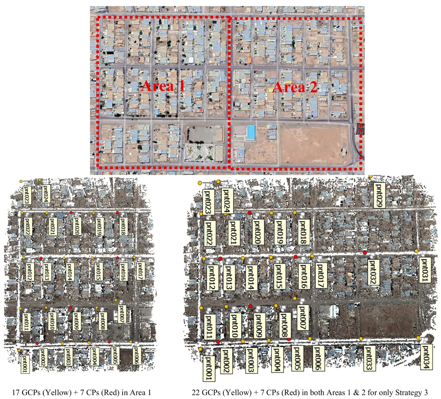
Figure 2. The (above) overview of the two urban test areas (Area 1 and Area 2; approximately 20 ha each) is characterized by predominantly low-rise buildings. Area 1 was used in all scenarios, whereas Area 2 was used only in Scenario 3. (Below) are the number and distributions of GCPs and CPs for all strategies in Area 1 and strategy 3 in Areas 1 & 2.
3.2. Ground Control Point (GCP) Design and Measurement
Ground control points were designed to ensure the geometric stability of the photogrammetric block and reliable independent accuracy assessment. As shown in Figure 2 below, in Area 1 (approximately 20 ha), GCPs were distributed with an average spacing of about 50 m, resulting in 24 GCPs. In Area 2, which used exclusively for partial high-overlap calibration experiments (strategy 3), 5 additional GCPs were measured. In total, 29 GCPs were designed and measured across the two study areas.
GCP locations were selected prior to fieldwork using the project boundary in a GIS environment to ensure uniform spatial distribution. Targets consisted of clearly visible artificial or natural features, including spray-painted ground targets in urban areas and prefabricated targets on unpaved surfaces. All GCP coordinates were measured using RTK-DGPS, providing centimeter-level positional accuracy.
As shown in Figure 2, the number and spatial distribution of GCPs were determined considering the block extent, the achieved GSD (2.6–4.6 cm), and standard UAV photogrammetric network design recommendations [15]. This configuration provides sufficient redundancy for stable bundle adjustment while avoiding unnecessary field-survey effort.
3.3. Flight Projects and Data Acquisition
Five network design scenarios were defined to evaluate different cost-reduction strategies in UAV photogrammetric missions systematically:
-
-
Scenario 1: Reduction of lateral overlap compensated by increased longitudinal overlap.
-
-
Scenario 2: Reduction of lateral overlap compensated by cross-flight acquisition.
-
-
Scenario 3: Partial high-overlap coverage for camera calibration combined with low-overlap coverage of the full area.
-
-
Scenario 4: Reduction of lateral overlap compensated by supplementary high-altitude acquisition.
-
-
Scenario 5: Reduction of lateral overlap compensated by oblique cross-flight imagery.
Each scenario was implemented through multiple sub-block configurations generated from the available flight datasets, allowing a controlled comparison of cost, completeness, and accuracy [12] relative to the high-overlap reference configuration.
3.4. Cost Indicator Definition
Normalized Cost Indices (Flight and Processing): Because absolute processing time depends on the specific hardware and SfM implementation, we report relative cost indices normalized to a reference block (Ref) with the highest image count and highest reconstruction quality. For each configuration $$i$$, the normalized total cost index is defined as:
| ```latex{\text{Cost}}_{i}=\frac{\left({\text{FC}}_{i}+\frac{{\text{PC}}_{i}}{4}\right)}{{\mathrm{C}\mathrm{o}\mathrm{s}\mathrm{t}}_{\mathrm{R}\mathrm{e}\mathrm{f}}}``` | (1) |
where $$\text{FC}$$ and $$\text{PC}$$ denote the flight-cost and processing-cost components, respectively. The factor $$1/4\mathrm{ }$$ is used to balance the magnitudes of the processing term and the flight term in the combined index. Flight cost (normalized):
| ```latex{\text{FC}}_{i}=\frac{\left(\frac{{\text{ALNI}}_{i}}{{V}_{i}}\right)}{{\mathrm{F}\mathrm{C}}_{\mathrm{R}\mathrm{e}\mathrm{f}}}``` | (2) |
where $$V$$ is the UAV flight velocity (m/s) and $$\text{ALNI}$$ is the Average Lateral Number of Images, defined from sidelap $${p}_{y}$$(%) as:
| ```latex{\text{ALNI}}_{i}=\frac{100}{100-{p}_{y,i}}``` | (3) |
with $${p}_{y}$$ being the image sidelap percentage in the lateral direction. Processing cost (normalized):
| ```latex{\text{PC}}_{i}=\frac{{NoI}_{i}}{{NoI}_{\text{Ref}}}``` | (4) |
where $$NoI$$ is the number of images in the block. Accordingly, the normalized processing cost index is defined as proportional to image count (NoI), which functions as a hardware-independent proxy for computational effort. Section 4.7 validates this assumption through empirical correlation with measured end-to-end processing times. All intermediate computations and parameter mappings for all configurations are documented in the Supplementary Excel file for full transparency.
3.5. Network Quality Assessment Criteria
The quality of each photogrammetric network configuration was evaluated using two complementary indicators: accuracy CA and completeness CM [13,15,16].
| ```latex{\text{Q}}_{i}=\frac{{C}_{Mi}/{C}_{Ai}}{{Q}_{\text{Ref}}}``` | (5) |
Completeness CM was quantified using the total number of reconstructed tie points after removing two-view points, serving as a proxy for network redundancy and geometric robustness. It should be emphasized that the tie-point count is not a direct measure of geometric accuracy. Rather, it serves as an indirect indicator of information richness and matching success within the image network. A higher number of tie points generally reflects more stable image correspondences and a lower likelihood of surface gaps or missing details; however, it does not guarantee metric correctness of the reconstructed surface.
Accuracy was assessed using independent checkpoints (CPs) and quantified by the combined accuracy index CA, defined as (1).
| $$C_A = \sqrt{(GSD \cdot RES_i)^2 + RMSE_{XYZ}^2},$$ | (6) |
where RESi denotes the image residuals at checkpoints, and RMSEXYZ represents the three-dimensional ground error at the same points. Image residuals were converted to ground units using the corresponding GSD to ensure metric consistency. This formulation avoids over-reliance on either image-space residuals or object-space RMSE alone and provides a balanced representation of geometric consistency across domains.
These indicators are directly reported in the Results section and form the basis of all quantitative comparisons among the tested mission configurations.
4. Experimental Results
4.1. Baseline Network Performance
The reference mission configuration in Table 1 is characterized by high longitudinal and lateral overlaps (80%–80%) and includes nadir, cross-flight, and oblique imagery acquired at a single flight altitude. This configuration provides strong geometric robustness and serves as the benchmark for all cost-oriented scenarios [12,17].
The baseline bundle adjustment yields low residuals at both GCPs and CPs, confirming that the control configuration supports stable estimation for subsequent comparisons.
Table 1. Specifications and aerial triangulation results of the reference (baseline) network configuration.
|
Item |
Value |
|---|---|
|
Nadir cross-flight |
Yes |
|
Oblique cross-flight |
Yes |
|
Number of images |
3823 |
|
Number of tie points |
1,865,865 |
|
Number of GCPs |
17 |
|
Number of CPs |
7 |
|
Nadir overlap (Endlap/Sidelap, %) |
95/80 |
|
Oblique overlap (Endlap/Sidelap, %) |
80/80 |
|
GCP RMSEXYZ (cm) |
2.93 |
|
CP RMSEXYZ (cm) |
2.95 |
|
GCP image residual STDExy (pix) |
0.58 |
|
CP image residual STDExy (pix) |
0.5 |
4.2. Scenario 1: Reduced Lateral Overlap with Increased Longitudinal Overlap
In Scenario 1, the network design aimed to reduce flight costs by decreasing the lateral overlap, while compensating for the resulting network weakness through an increase in longitudinal overlap. A total of 32 sub-block configurations were designed and processed in this scenario. After filtering and excluding several sub-blocks due to either low completeness indices or high cost indices, a total of ten sub-blocks remained for further analysis. Based on a relative comparison among these candidates, sub-blocks 17 and 11 in Scenario 1 were ultimately selected for stereoscopic mapping and OIM generation (Table 2). The remaining configurations were not selected because, in comparison with the chosen sub-blocks, they did not offer a favorable balance between accuracy, completeness, and cost, and therefore did not meet the prioritization criteria.
These results indicate that increasing longitudinal overlap alone cannot fully compensate for the loss of geometric strength caused by reduced lateral overlap. While acceptable accuracy can be maintained for mapping products, network completeness deteriorates rapidly, limiting suitability for dense 3D reconstruction.
4.3. Scenario 2: Cross-Flight Configuration
In Scenario 2, the network was designed to reduce flight costs by decreasing the lateral overlap, while compensating for the weakened geometry through cross-flight acquisition [18]. Similar to Scenario 1, 32 sub-block configurations were designed and processed. As shown in Table 3 (Scenario 2 results), 30 out of the 32 configurations exhibited either high cost indices or completeness values below 0.25, leaving only Sub-blocks 13 and 17 as viable candidates. Given their marginal completeness levels, these two configurations are recommended only for mapping and OIM production and were found to be unsuitable for 3D mesh generation.
It should be noted that, based on the total cost reduction column in Table 3, configurations with cost indices greater than 0.6 were initially excluded from processing. However, since this cost index was predictive rather than based on actual processing measurements, and because all field-acquired datasets were available for laboratory analysis—allowing a comprehensive assessment of system behavior—all configurations in Scenarios 1 and 2 were processed. For subsequent scenarios, due to the substantial computational demand and time constraints, this exhaustive approach was abandoned, and only logically feasible sub-block configurations with cost indices below 1 were selected for processing.
Table 2. Detailed evaluation of aerial triangulation results for different longitudinal and lateral overlap configurations in Scenario 1, as Reduced Lateral Overlap with Increased Longitudinal Overlap. The final accuracy, completeness, and cost indices relative to the 80–80 reference configuration used for configuration assessment.
|
No. |
Longitudinal Overlap (%) |
Lateral Overlap (%) |
Number of Images |
UAV Speed (m/s) |
Relative Flight Cost |
Relative Processing Cost |
Accuracy |
Completeness |
Cost |
Remarks |
|---|---|---|---|---|---|---|---|---|---|---|
|
1 |
60 |
20 |
74 |
15.0 |
0.1 |
0.2 |
1.3 |
0.1 |
0.1 |
Rejected for low Completeness |
|
2 |
60 |
40 |
79 |
15.0 |
0.2 |
0.2 |
1.2 |
0.0 |
0.2 |
Rejected for low Completeness |
|
3 |
60 |
60 |
114 |
15.0 |
0.3 |
0.3 |
1.0 |
0.1 |
0.3 |
Rejected for low Completeness |
|
4 |
60 |
80 |
193 |
15.0 |
0.5 |
0.5 |
1.3 |
0.3 |
0.5 |
Not recommended |
|
5 |
65 |
20 |
70 |
13.1 |
0.1 |
0.2 |
0.9 |
0.1 |
0.2 |
Rejected for low Completeness |
|
6 |
65 |
40 |
83 |
13.1 |
0.2 |
0.2 |
1.0 |
0.1 |
0.2 |
Rejected for low Completeness |
|
7 |
65 |
60 |
123 |
13.1 |
0.3 |
0.3 |
1.1 |
0.2 |
0.3 |
Rejected for low Completeness |
|
8 |
65 |
80 |
235 |
13.1 |
0.6 |
0.7 |
1.1 |
0.5 |
0.6 |
Not recommended |
|
9 |
70 |
20 |
70 |
11.3 |
0.2 |
0.2 |
1.0 |
0.2 |
0.2 |
Rejected for low Completeness |
|
10 |
70 |
40 |
84 |
11.3 |
0.2 |
0.2 |
0.7 |
0.2 |
0.2 |
Rejected for low Completeness |
|
11 |
70 |
60 |
124 |
11.3 |
0.3 |
0.4 |
0.9 |
0.4 |
0.3 |
Recommended for MAP & OIM |
|
12 |
70 |
80 |
237 |
11.3 |
0.7 |
0.7 |
0.9 |
0.5 |
0.7 |
Rejected for high Cost |
|
13 |
75 |
20 |
85 |
9.3 |
0.2 |
0.2 |
0.6 |
0.1 |
0.2 |
Rejected for low Completeness |
|
14 |
75 |
40 |
103 |
9.3 |
0.3 |
0.3 |
0.7 |
0.2 |
0.3 |
Rejected for low Completeness |
|
15 |
75 |
60 |
152 |
9.3 |
0.4 |
0.4 |
0.9 |
0.3 |
0.4 |
Not recommended |
|
16 |
75 |
80 |
289 |
9.3 |
0.8 |
0.8 |
0.8 |
0.7 |
0.8 |
Rejected for high Cost |
|
17 |
80 |
20 |
103 |
7.5 |
0.3 |
0.3 |
1.0 |
0.4 |
0.3 |
Recommended for MAP |
|
18 |
80 |
40 |
125 |
7.5 |
0.3 |
0.4 |
1.2 |
0.5 |
0.3 |
Not recommended |
|
19 |
80 |
60 |
187 |
7.5 |
0.5 |
0.5 |
1.2 |
0.7 |
0.5 |
Not recommended |
|
20 |
80 |
80 |
354 |
7.5 |
1.0 |
1.0 |
1.0 |
1.0 |
1.0 |
Reference * |
|
21 |
85 |
20 |
139 |
5.5 |
0.3 |
0.4 |
1.3 |
0.5 |
0.4 |
Not recommended |
|
22 |
85 |
40 |
168 |
5.5 |
0.5 |
0.5 |
1.3 |
0.5 |
0.5 |
Not recommended |
|
23 |
85 |
60 |
251 |
5.5 |
0.7 |
0.7 |
1.2 |
0.8 |
0.7 |
Rejected for high Cost |
|
24 |
85 |
80 |
475 |
5.5 |
1.4 |
1.3 |
1.1 |
1.2 |
1.4 |
Rejected for high Cost |
|
25 |
90 |
20 |
212 |
3.7 |
0.5 |
0.6 |
0.8 |
0.7 |
0.5 |
Not recommended |
|
26 |
90 |
40 |
255 |
3.7 |
0.7 |
0.7 |
1.1 |
0.8 |
0.7 |
Rejected for high Cost |
|
27 |
90 |
60 |
383 |
3.7 |
1.0 |
1.1 |
1.2 |
1.2 |
1.0 |
Rejected for high Cost |
|
28 |
90 |
80 |
723 |
3.7 |
2.0 |
2.0 |
1.0 |
1.8 |
2.0 |
Rejected for high Cost |
|
29 |
95 |
20 |
512 |
2.0 |
0.9 |
1.4 |
0.8 |
0.9 |
1.0 |
Rejected for high Cost |
|
30 |
95 |
40 |
606 |
2.0 |
1.3 |
1.7 |
1.1 |
1.1 |
1.3 |
Rejected for high Cost |
|
31 |
95 |
60 |
863 |
2.0 |
1.9 |
2.4 |
1.1 |
1.6 |
2.0 |
Rejected for high Cost |
|
32 |
95 |
80 |
1572 |
2.0 |
3.8 |
4.4 |
1.1 |
2.6 |
3.9 |
Rejected for high Cost |
* The The gray row represents the reference block. Values of Relative Flight Cost, Relative Processing Cost, Accuracy, Completeness and Cost were calculated with respect to this reference using Equation (1), Equation (2), Equation (4), and Equation (5).
Table 3. Detailed evaluation of aerial triangulation results for different longitudinal and lateral overlap configurations in Scenario 2 as Cross-Flight Configuration. The final accuracy, completeness, and cost indices relative to the 80–80 reference configuration used for configuration assessment.
|
No. |
Longitudinal Overlap (%) |
Lateral Overlap (%) |
Number of Images |
UAV Speed (m/s) |
Relative Flight Cost |
Relative Processing Cost |
Accuracy |
Completeness |
Cost |
Remarks |
|---|---|---|---|---|---|---|---|---|---|---|
|
1 |
60 |
20 |
128 |
9.1 |
0.4 |
0.4 |
1.1 |
0.1 |
0.4 |
Rejected for low Completeness |
|
2 |
60 |
40 |
145 |
10.0 |
0.5 |
0.4 |
0.6 |
0.1 |
0.5 |
Rejected for low Completeness |
|
3 |
60 |
60 |
207 |
11.0 |
0.7 |
0.6 |
1.0 |
0.2 |
0.7 |
Rejected for low Completeness |
|
4 |
60 |
80 |
377 |
12.0 |
1.3 |
1.1 |
0.9 |
0.6 |
1.2 |
Rejected for high Cost |
|
5 |
65 |
20 |
141 |
13.1 |
0.3 |
0.4 |
0.8 |
0.1 |
0.3 |
Rejected for low Completeness |
|
6 |
65 |
40 |
172 |
13.1 |
0.4 |
0.5 |
1.0 |
0.2 |
0.4 |
Rejected for low Completeness |
|
7 |
65 |
60 |
241 |
13.1 |
0.6 |
0.7 |
0.8 |
0.2 |
0.6 |
Rejected for low Completeness |
|
8 |
65 |
80 |
473 |
13.1 |
1.1 |
1.3 |
0.7 |
0.5 |
1.2 |
Rejected for high Cost |
|
9 |
70 |
20 |
152 |
11.3 |
0.3 |
0.4 |
1.0 |
0.2 |
0.4 |
Rejected for low Completeness |
|
10 |
70 |
40 |
184 |
11.3 |
0.4 |
0.5 |
0.6 |
0.2 |
0.5 |
Rejected for low Completeness |
|
11 |
70 |
60 |
257 |
11.3 |
0.7 |
0.7 |
0.8 |
0.2 |
0.7 |
Rejected for low Completeness |
|
12 |
70 |
80 |
494 |
11.3 |
1.3 |
1.4 |
0.8 |
3.5 |
1.3 |
Rejected for high Cost |
|
13 |
75 |
20 |
177 |
9.3 |
0.4 |
0.5 |
0.8 |
0.3 |
0.4 |
Recommended for MAP & OIM |
|
14 |
75 |
40 |
219 |
9.3 |
0.5 |
0.6 |
0.7 |
0.2 |
0.6 |
Rejected for low Completeness |
|
15 |
75 |
60 |
323 |
9.3 |
0.8 |
0.9 |
0.7 |
0.4 |
0.8 |
Rejected for high Cost |
|
16 |
75 |
80 |
289 |
9.3 |
1.6 |
0.8 |
0.6 |
3.8 |
1.5 |
Rejected for high Cost |
|
17 |
80 |
20 |
215 |
7.5 |
0.5 |
0.6 |
0.9 |
0.3 |
0.5 |
Recommended for MAP & OIM |
|
18 |
80 |
40 |
261 |
7.5 |
0.7 |
0.7 |
0.8 |
0.3 |
0.7 |
Rejected for high Cost |
|
19 |
80 |
60 |
380 |
7.5 |
1.0 |
1.1 |
0.7 |
0.5 |
1.0 |
Rejected for high Cost |
|
20 |
80 |
80 |
734 |
7.5 |
2.0 |
2.1 |
0.7 |
1.2 |
2.0 |
Rejected for high Cost |
|
21 |
85 |
20 |
139 |
5.5 |
0.7 |
0.4 |
1.0 |
0.5 |
0.6 |
Rejected for high Cost |
|
22 |
85 |
40 |
346 |
5.5 |
0.9 |
1.0 |
0.7 |
0.7 |
0.9 |
Rejected for high Cost |
|
23 |
85 |
60 |
501 |
5.5 |
1.4 |
1.4 |
0.8 |
1.2 |
1.4 |
Rejected for high Cost |
|
24 |
85 |
80 |
974 |
5.5 |
2.7 |
2.8 |
0.7 |
1.1 |
2.7 |
Rejected for high Cost |
|
25 |
90 |
20 |
460 |
3.7 |
1.0 |
1.3 |
1.0 |
0.4 |
1.1 |
Rejected for high Cost |
|
26 |
90 |
40 |
552 |
3.7 |
1.4 |
1.6 |
0.7 |
0.6 |
1.4 |
Rejected for high Cost |
|
27 |
90 |
60 |
785 |
3.7 |
2.0 |
2.2 |
0.7 |
0.6 |
2.1 |
Rejected for high Cost |
|
28 |
90 |
80 |
1449 |
3.7 |
4.1 |
4.1 |
0.8 |
2.7 |
4.1 |
Rejected for high Cost |
|
29 |
95 |
20 |
913 |
2.0 |
1.9 |
2.6 |
1.5 |
3.4 |
2.0 |
Rejected for high Cost |
|
30 |
95 |
40 |
1093 |
2.0 |
2.5 |
3.1 |
1.4 |
3.7 |
2.6 |
Rejected for high Cost |
|
31 |
95 |
60 |
1558 |
2.0 |
3.8 |
4.4 |
1.1 |
3.4 |
3.9 |
Rejected for high Cost |
|
32 |
95 |
80 |
2961 |
2.0 |
7.5 |
8.4 |
1.0 |
4.4 |
7.7 |
Rejected for high Cost |
4.4. Scenario 3: Partial High-Overlap Coverage
In Scenario 3, a small subset of the study area was initially flown with high overlap to perform camera calibration [19]. Subsequently, the main flight was conducted under the assumption that the camera calibration parameters were known, to evaluate whether the lateral overlap could be reduced without a significant loss in accuracy. Four sub-block configurations were designed and processed in this scenario. According to Table 4, all sub-blocks exhibit a degradation in accuracy; however, Sub-block 1 provides a substantial cost reduction with only a marginal decrease in accuracy and is therefore suitable for stereoscopic mapping.
The observed accuracy degradation suggests that partial high-overlap calibration cannot fully compensate for the weakened block geometry when the majority of the area is covered with low lateral overlap.
Table 4. Detailed evaluation of aerial triangulation results for different lateral overlap configurations in Scenario 3 as Partial High-Overlap Coverage. The final accuracy, completeness, and cost indices relative to the 80–80 reference configuration used for configuration assessment.
|
No. |
Longitudinal Overlap (%) |
Lateral Overlap (%) |
Number of Images |
UAV Speed (m/s) |
Relative Flight Cost |
Relative Processing Cost |
Accuracy |
Completeness |
Cost |
Remarks |
|---|---|---|---|---|---|---|---|---|---|---|
|
1 |
80 |
20 |
103 |
7.5 |
0.3 |
0.3 |
1.1 |
0.4 |
0.3 |
Recommended for MAP |
|
2 |
80 |
40 |
125 |
7.5 |
0.3 |
0.4 |
1.1 |
0.5 |
0.3 |
Not recommended |
|
3 |
80 |
60 |
187 |
7.5 |
0.5 |
0.5 |
1.3 |
0.7 |
0.5 |
Not recommended |
|
4 |
80 |
80 |
354 |
7.5 |
1.0 |
1.0 |
1.3 |
1.0 |
1.0 |
Rejected due to high Cost |
4.5. Scenario 4: Multi-Altitude Acquisition
In Scenario 4, in order to compensate for the reduction in lateral overlap, an additional flight was conducted at twice the nominal flight altitude with high overlap [8]. It should be noted that doubling the flight altitude reduces the number of flight strips by half and decreases the total number of images by approximately a factor of four, while the additional costs associated with this supplementary flight remain marginal. Overall, twelve sub-block configurations were designed and processed in this scenario, and the corresponding parameters and performance indices are presented in Table 5.
Based on the results reported in Table 5, Sub-blocks 1, 4, and 5 were selected as the most favorable configurations in terms of cost, completeness, and accuracy. Sub-block 1 exhibits a very low cost while achieving an accuracy level comparable to the 80–80 reference block. Sub-block 4 represents a distinctive configuration that not only yields a substantial cost reduction but also demonstrates a pronounced improvement in completeness, making it particularly suitable for 3D mesh generation. The observed increase in tie-point count indicates improved image matching stability and a richer set of geometric constraints, which reduces the likelihood of surface gaps or missing façade details. However, tie-point density alone does not guarantee geometric fidelity of the reconstructed surface; it primarily reflects reconstruction completeness rather than metric accuracy. Although Sub-block 5 entails a higher cost than Sub-block 1, it provides a greater improvement in accuracy and is therefore recommended for mapping purposes. Nevertheless, none of these three configurations is recommended for OIM production, as their lateral overlap remains below 60%.
None of the evaluated configurations in this scenario is recommended for OIM production, as lateral overlaps below 60% are insufficient to ensure radiometric consistency and seamless mosaic generation.
Table 5. Detailed evaluation of aerial triangulation results for different second higher network lateral overlap configurations in Scenario 4 as Multi-Altitude Acquisition. The final accuracy, completeness, and cost indices relative to the 80–80 reference configuration used for configuration assessment (HN = Higher Altitude Network).
|
No. |
Longitudinal Overlap (%) |
Lateral Overlap (%) |
HN Longitudinal Overlap (%) |
HN Lateral Overlap (%) |
Number of Images |
UAV Speed (m/s) |
HN UAV Speed (m/s) |
Relative Flight Cost |
Relative Processing Cost |
Accuracy |
Completeness |
Cost |
Remarks |
|---|---|---|---|---|---|---|---|---|---|---|---|---|---|
|
1 |
60 |
20 |
80 |
20 |
123 |
15.0 |
15.0 |
0.2 |
0.3 |
1.0 |
0.2 |
0.2 |
Recommended for MAP |
|
2 |
60 |
20 |
80 |
40 |
135 |
15.0 |
15.0 |
0.2 |
0.4 |
1.1 |
0.4 |
0.2 |
Not recommended |
|
3 |
60 |
20 |
80 |
60 |
165 |
15.0 |
15.0 |
0.3 |
0.5 |
1.3 |
0.6 |
0.3 |
Not recommended |
|
4 |
60 |
20 |
80 |
80 |
234 |
15.0 |
15.0 |
0.4 |
0.7 |
1.1 |
1.3 |
0.4 |
Recommended for MAP |
|
5 |
80 |
20 |
80 |
20 |
152 |
7.5 |
15.0 |
0.3 |
0.4 |
0.7 |
0.5 |
0.3 |
Not recommended |
|
6 |
80 |
20 |
80 |
40 |
164 |
7.5 |
15.0 |
0.3 |
0.5 |
0.9 |
0.5 |
0.4 |
Recommended for 3D Mesh |
|
7 |
80 |
20 |
80 |
60 |
196 |
7.5 |
15.0 |
0.4 |
0.6 |
1.1 |
0.5 |
0.4 |
Not recommended |
|
8 |
80 |
20 |
80 |
80 |
264 |
7.5 |
15.0 |
0.5 |
0.7 |
1.1 |
1.3 |
0.5 |
Not recommended |
|
9 |
95 |
20 |
80 |
20 |
586 |
2.0 |
15.0 |
1.0 |
1.7 |
1.1 |
0.7 |
1.1 |
Rejected for high Cost |
|
10 |
95 |
20 |
80 |
40 |
598 |
2.0 |
15.0 |
1.0 |
1.7 |
0.8 |
0.6 |
1.2 |
Rejected for high Cost |
|
11 |
95 |
20 |
80 |
60 |
628 |
2.0 |
15.0 |
1.1 |
1.8 |
1.0 |
0.8 |
1.2 |
Rejected for high Cost |
|
12 |
95 |
20 |
80 |
80 |
698 |
2.0 |
15.0 |
1.2 |
2.0 |
0.9 |
1.5 |
1.3 |
Rejected for high Cost |
4.6. Scenario 5: Integration of Oblique Imagery
In this scenario, both nadir and oblique imaging strategies were investigated. Nadir and oblique images were acquired along north–south as well as east–west flight directions. Although full 3D mesh generation typically requires oblique imagery in both directions to capture four viewing angles—considering the zigzag flight pattern of a multirotor UAV—only one oblique viewing direction was combined with nadir imagery in order to avoid additional flight costs. Consequently, in Scenario 5, nadir images were independently combined with parallel and perpendicular oblique images under different overlap configurations and processed accordingly.
A total of 18 sub-block configurations were designed and processed in this scenario, and their accuracy, completeness, and cost indices were computed as reported in Table 6. Fifteen sub-blocks were discarded due to either high cost indices or low completeness values, leaving three candidate configurations. Among these, Sub-block 12 was selected as the optimal configuration, as it provides an appropriate balance between cost and accuracy while maintaining a lateral overlap of 60%, and is therefore recommended for stereoscopic mapping and OIM production.
Although oblique imagery substantially improves network completeness and geometric robustness, the recommendations for dense 3D mesh reconstruction are based on completeness indicators rather than explicit mesh quality metrics. Recommendations for dense 3D mesh generation are based on network completeness and geometric robustness indicators rather than direct mesh-quality metrics; therefore, local surface artifacts may still arise depending on scene complexity.
4.7. Processing Time Analysis and Correlation with Image-Count Proxy
In practice, total processing time in UAV photogrammetry is influenced by multiple interacting factors, including data preparation and block definition, image feature extraction and matching for initial block formation, manual and semi-automatic marking of ground control and check points, filtering of outlier image observations, navigation data and GCPs coordinates, repeated bundle adjustments, parameter dependency removal, global and thematic weight refinement, and iterative quality control. Consequently, absolute processing time cannot be represented by a single triangulation run alone.
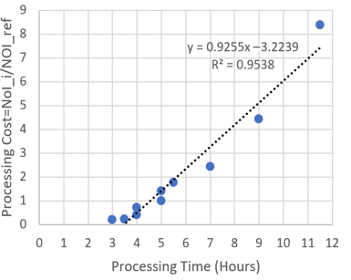
For this reason, measured end-to-end processing times were recorded for a set of representative configurations spanning low, medium, and high image counts. Table 7 summarizes the number of images and the corresponding total processing time (including iterative adjustments and quality control steps) for a limited number of our block processing times in practice. A correlation analysis was then performed between the relative number of images (NoIi/NoIRef) and the measured relative processing time (Ti). The results indicate a strong positive correlation (R2 = 0.95), confirming that image count acts as a dominant predictor of relative processing effort across configurations.
From extensive practical experience across hundreds of real UAV projects, it is observed that as image count increases, not only do matching and MVS operations grow, but the number of GCP observations, navigation constraints, interactive refinement steps, and iterative adjustments also increase proportionally. Therefore, even though processing time is influenced by multiple factors, relative image count remains the key implicit parameter governing relative processing duration between blocks.
Table 6. Detailed evaluation of aerial triangulation results for lateral overlap configurations of combined vertical and oblique networks in Scenario 5. The final accuracy, completeness, and cost indices relative to the 80–80 reference configuration used for configuration assessment. (ON = Oblique Network).
|
No. |
Longitudinal Overlap (%) |
Lateral Overlap (%) |
ON Longitudinal Overlap (%) |
ON Lateral Overlap (%) |
ON Orientation |
Number of Images |
UAV Speed (m/s) |
ON UAV Speed (m/s) |
Relative Flight Cost |
Relative Processing Cost |
Accuracy |
Completeness |
Cost |
Remarks |
|---|---|---|---|---|---|---|---|---|---|---|---|---|---|---|
|
1 |
60 |
20 |
80 |
60 |
Par |
260 |
15.0 |
7.5 |
0.6 |
0.7 |
1.0 |
0.7 |
0.6 |
Rejected for high Cost |
|
2 |
60 |
40 |
80 |
40 |
Par |
190 |
15.0 |
7.5 |
0.5 |
0.5 |
0.8 |
0.3 |
0.5 |
Not recommended |
|
3 |
60 |
60 |
80 |
20 |
Par |
204 |
15.0 |
7.5 |
0.5 |
0.6 |
0.8 |
0.4 |
0.5 |
Not recommended |
|
4 |
80 |
20 |
80 |
60 |
Par |
295 |
7.5 |
7.5 |
0.8 |
0.8 |
1.1 |
0.8 |
0.8 |
Rejected for high Cost |
|
5 |
80 |
40 |
80 |
40 |
Par |
258 |
7.5 |
7.5 |
0.7 |
0.7 |
0.9 |
0.5 |
0.7 |
Rejected for high Cost |
|
6 |
80 |
60 |
80 |
20 |
Par |
305 |
7.5 |
7.5 |
0.8 |
0.9 |
1.1 |
0.7 |
0.8 |
Rejected for high Cost |
|
7 |
90 |
20 |
80 |
60 |
Par |
432 |
3.7 |
7.5 |
1.0 |
1.2 |
1.0 |
0.9 |
1.0 |
Rejected for high Cost |
|
8 |
90 |
40 |
80 |
40 |
Par |
414 |
3.7 |
7.5 |
1.0 |
1.2 |
1.0 |
0.6 |
1.0 |
Rejected for high Cost |
|
9 |
90 |
60 |
80 |
20 |
Par |
516 |
3.7 |
7.5 |
1.3 |
1.5 |
1.1 |
0.7 |
1.3 |
Rejected for high Cost |
|
10 |
60 |
20 |
80 |
60 |
Pen |
214 |
15.0 |
7.5 |
0.6 |
0.6 |
1.1 |
0.4 |
0.6 |
Rejected for high Cost |
|
11 |
60 |
40 |
80 |
40 |
Pen |
165 |
15.0 |
7.5 |
0.5 |
0.5 |
1.0 |
0.2 |
0.5 |
Rejected for low Completeness |
|
12 |
60 |
60 |
80 |
20 |
Pen |
182 |
15.0 |
7.5 |
0.5 |
0.5 |
0.7 |
0.3 |
0.5 |
Recommended for MAP & OIM |
|
13 |
80 |
20 |
80 |
60 |
Pen |
252 |
7.5 |
7.5 |
0.8 |
0.7 |
1.0 |
0.5 |
0.7 |
Rejected for high Cost |
|
14 |
80 |
40 |
80 |
40 |
Pen |
233 |
7.5 |
7.5 |
0.7 |
0.7 |
1.1 |
0.4 |
0.7 |
Rejected for high Cost |
|
15 |
80 |
60 |
80 |
20 |
Pen |
283 |
7.5 |
7.5 |
0.8 |
0.8 |
0.9 |
0.5 |
0.8 |
Rejected for high Cost |
|
16 |
90 |
20 |
80 |
60 |
Pen |
386 |
3.7 |
7.5 |
1.0 |
1.1 |
1.0 |
0.7 |
1.0 |
Rejected for high Cost |
|
17 |
90 |
40 |
80 |
40 |
Pen |
389 |
3.7 |
7.5 |
1.0 |
1.1 |
1.1 |
0.8 |
1.0 |
Rejected for high Cost |
|
18 |
90 |
60 |
80 |
20 |
Pen |
494 |
3.7 |
7.5 |
1.3 |
1.4 |
1.1 |
0.6 |
1.3 |
Rejected for high Cost |
Table 7. The Pearson correlation coefficient between relative image count and relative processing time was 0.975 (R2 = 0.95), demonstrating that the image-count proxy reliably predicts relative computational effort (the row in gray with # 20 is the Reference case).
|
Test No. in Scenario |
Scenario |
Longitudinal Overlap (%) |
Lateral Overlap (%) |
Number of Images |
Real Processing Time (hours) |
Relative Processing Cost |
 |
|
5 |
1 |
65 |
20 |
70 |
3.0 |
0.20 |
|
|
6 |
1 |
65 |
40 |
83 |
3.5 |
0.23 |
|
|
2 |
2 |
60 |
40 |
145 |
4.0 |
0.41 |
|
|
11 |
2 |
70 |
60 |
257 |
4.0 |
0.73 |
|
|
20 * |
1 |
80 |
80 |
354 |
5.0 |
1.00 |
|
|
12 |
2 |
70 |
80 |
494 |
5.0 |
1.40 |
|
|
11 |
4 |
95 |
20 |
628 |
5.5 |
1.77 |
|
|
31 |
1 |
95 |
60 |
863 |
7.0 |
2.44 |
|
|
32 |
1 |
95 |
80 |
1572 |
9.0 |
4.44 |
|
|
32 |
2 |
95 |
80 |
2961 |
11.5 |
8.36 |
* The The gray row represents the reference block (See footnote of Table 2).
4.8. Comparative Cost–Quality Analysis
In this study, the processing cost index is computed from the number of images that have a strong correlation to processing time, and then normalized to the reference block, i.e., $$\text{PC}={NoI}_{i}/{NoI}_{\text{Ref}}$$. This approach avoids reporting hardware-dependent absolute times while preserving relative scaling across configurations. The flight cost index is derived from sidelap-driven strip redundancy through $$\text{ALNI}=100/\left(100-{p}_{y}\right)$$ and the actual flight velocity, and is likewise normalized to the reference. A complete list of computations for all blocks is provided in the Supplementary Excel file.
In this section, all 98 configurations are first statistically evaluated and visualized in the quality–cost space shown in Figure 3. The quality metric reflects the amount of reconstructed geometric information per unit of accuracy loss, thereby favoring configurations that yield dense, stable networks without sacrificing checkpoint accuracy.
Since optimal solutions are characterized by higher quality and lower cost, the upper-left corner of Figure 3 represents the ideal point. Accordingly, configurations located closer to this point are considered more favorable. The reference network is positioned at coordinates (1, 1). All Pareto-front points located in the upper-right quadrant relative to this reference correspond to sub-networks with both higher quality and higher cost; these are predominantly 3D-mesh configurations labeled T, originating from Scenarios 1, 2, and 4. Conversely, Pareto-front points located in the lower-left quadrant of the reference point exhibit both reduced quality and reduced cost and are mainly associated with MAP and OIM configurations labeled M and O, derived from Scenarios 1, 2, 4, and 5.
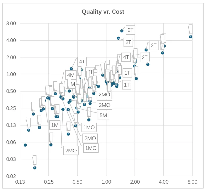
Figure 3. Quality–cost distribution for 98 sub-network configurations (logarithmic cost axis). The quality metric is defined as Q = C/A, where C is the normalized completeness index (tie-point count), and A is the normalized accuracy index (C_A); therefore, higher Q indicates higher completeness per unit accuracy cost. Labels indicate scenario number followed by M, O, and T for MAP, OIM, and 3D-oriented configurations, respectively.
Subsequently, the selected sub-blocks from all scenarios were comparatively evaluated to further narrow the search space and identify the most promising configurations. The analyses conducted across five scenarios identified nine sub-blocks that provided a more favorable balance between cost reduction and quality preservation or improvement, which are listed in Table 8 in descending order of cost improvement. Sub-blocks ranked higher in the table exhibit greater cost savings and were therefore initially prioritized. However, when the overlap in both directions falls below 60%, the network’s geometric strength deteriorates, limiting its ability to detect and correct distortions caused by non-metric camera instability. Consequently, sub-blocks 1, 2, 3, and 7 were excluded, unless very high camera stability and mean image residuals below 0.4 pixels could be guaranteed. Although the residuals observed across the 98 experiments ranged from 0.25 to 0.50 pixels, these four configurations were discarded to ensure the general applicability of the proposed strategy across different UAVs and camera systems.
Among the remaining five solutions, the maximum improvements in cost, completeness, and accuracy are highlighted in Table 5 and Table 6. The greatest cost reduction was achieved in Scenario 1, with 70% longitudinal and 60% lateral overlap, which is recommended for mapping and OIM generation, at approximately one-third the cost of the classical 80–80 configuration. The highest completeness improvement was obtained in Scenario 4, combining a 60–20 nadir flight with a high-altitude 80–80 flight, resulting in a 33% increase in point-cloud density while maintaining reduced image numbers and flight time; this configuration is therefore recommended for dense point-cloud and 3D mesh generation, but not for mapping products due to moderate geometric strength. The greatest 3D reconstruction accuracy improvement was observed in Scenario 5 (Row 8), where a hybrid nadir–oblique acquisition with effective 60–60 overlap enhanced network robustness and achieved a 33% accuracy improvement at half the cost of the 80–80 reference, making it suitable for mapping and orthophoto production.
From Scenario 2, two candidates (Rows 6 and 9) were retained. Row 6—an efficient cross-flight configuration with 75% longitudinal and 20% lateral overlap—was selected as the preferred option, achieving a 58% reduction in the normalized cost index and a 22% improvement in the checkpoint-based accuracy index (i.e., lower C_A) relative to the reference. However, it should be used with caution for ortho-image-mosaic (OIM) production, because cross-flight acquisitions are more susceptible to illumination and shadow inconsistencies unless missions are executed within a tightly controlled time window [20]. Overall, Scenarios 1, 4, and 5 provided the most favorable cost–quality trade-offs, whereas Scenarios 2 and 3 offered limited operational benefit under the tested conditions and the defined cost–quality constraints.
Table 8. Key flight parameters and normalized quality–cost metrics of the selected sub-blocks, including accuracy, completeness, cost, associated risk levels, and recommended applications.
|
No. |
Scenario No. |
Block No. within Scenario |
Nadir Flight Longitudinal Overlap (%) |
Nadir Flight Lateral Overlap (%) |
Second Flight Longitudinal Overlap (%) |
Second Flight Lateral Overlap (%) |
Oblique Flight Direction |
Accuracy Index |
Completeness Index |
Cost Index |
Accuracy Improvement (%) |
Completeness Improvement (%) |
Cost Improvement (%) |
Risk of Model Stepping and Irreversible Errors |
Recommended for Stereoscopic Mapping |
Recommended for OIM |
Recommended for 3D Mesh Generation |
|---|---|---|---|---|---|---|---|---|---|---|---|---|---|---|---|---|---|
|
1 |
4 |
1 |
60 |
20 |
80 |
20 |
— |
1.02 |
0.25 |
0.22 |
−2% |
−75% |
+78% |
High |
No |
No |
No |
|
2 |
1 |
17 |
80 |
20 |
— |
— |
— |
1.03 |
0.40 |
0.26 |
−3% |
−60% |
+74% |
High |
No |
No |
No |
|
3 |
3 |
1 |
80 |
20 |
— |
— |
— |
1.07 |
0.40 |
0.26 |
−7% |
−60% |
+74% |
High |
No |
No |
No |
|
4 |
1 |
11 |
70 |
60 |
— |
— |
— |
0.93 |
0.37 |
0.34 |
+7% |
−63% |
+66% |
Low |
Yes |
Yes |
No |
|
5 |
4 |
4 |
60 |
20 |
80 |
80 |
— |
1.07 |
1.34 |
0.36 |
−7% |
+34% |
+64% |
Medium |
No |
No |
Yes |
|
6 |
2 |
13 |
75 |
20 |
— |
— |
— |
0.78 |
0.27 |
0.42 |
+22% |
−73% |
+58% |
Low |
Yes |
No |
No |
|
7 |
4 |
5 |
80 |
20 |
80 |
20 |
— |
0.73 |
0.48 |
0.43 |
+27% |
−52% |
+57% |
High |
No |
No |
No |
|
8 |
5 |
12 |
60 |
60 |
80 |
20 |
Perpendicular |
0.67 |
0.27 |
0.50 |
+33% |
−73% |
+50% |
Low |
Yes |
Yes |
No |
|
9 |
2 |
17 |
80 |
20 |
— |
— |
— |
0.93 |
0.25 |
0.52 |
+7% |
−75% |
+48% |
Low |
Yes |
No |
No |
4.9. Summary of Results
Overall, the experiments confirm that substantial cost savings in UAV photogrammetry can be achieved through geometric reconfiguration of the imaging network rather than by redundancy increase alone. Across the evaluated configurations, several candidate sub-blocks achieved approximately ≥50% normalized cost reduction while maintaining checkpoint-based accuracy comparable to the high-overlap reference (Table 8).
The results further indicate that mission design should be product-dependent. For vector mapping (MAP), reliable performance can be achieved with low lateral overlap (down to ~20%) provided that longitudinal overlap remains sufficient and the network is not pushed below the geometric stability threshold. For OIM production, both longitudinal and lateral overlaps should be at least moderate (typically ≥60%) to support consistent matching and seamless mosaicking. In contrast, dense 3D reconstruction requires a stronger geometric configuration, and benefits most from cross-flight and oblique imagery in addition to nadir views, with overlap levels exceeding 60% and preferably approaching 80%.
These findings provide a quantitative basis for cost-aware, autonomous mission planning, in which flight geometry and overlap are selected based on the target product and acceptable accuracy–cost trade-offs.
5. Discussion
5.1. Implications for Autonomous UAV Mission Planning
The results indicate that cost-efficient UAV photogrammetry cannot be achieved by overlap reduction alone; it requires deliberate restructuring of the image network to preserve geometric strength [21,22]. For autonomous and semi-autonomous mission planners, this implies that flight planning should move beyond redundancy-driven heuristics and explicitly account for geometric robustness [20,23]. Accordingly, an autonomy-aware planner can operationalize cost awareness by controlling the dominant cost drivers—strip count and image count—via overlap allocation and geometry strengthening, while enforcing product-dependent quality thresholds. Recent comprehensive surveys have summarized state-of-the-art methodologies in mission planning for autonomous UAV systems, particularly focusing on task assignment and path planning techniques that are foundational for autonomous operation and multi-UAV coordination [4].
In practice, planners may incorporate geometry-aware criteria—such as ray-intersection diversity and DOP-like measures [23]—together with task-specific constraints (e.g., orthomosaic versus 3D mapping). The cost–accuracy trade-off analysis further suggests the existence of Pareto-optimal mission configurations, enabling goal-driven planning in which overlap, viewing geometry, and altitude are selected based on accuracy requirements and resource limits rather than fixed, conservative defaults.
From an autonomous mission-planning pers pective, the experimental results enable the formulation of rule-based and Pareto-driven decision policies linking mission objectives to cost–quality constraints. For instance, when the target product is vector mapping (MAP) and the normalized cost constraint is below approximately 0.4, mission configurations resembling Scenario 1—characterized by reduced lateral overlap compensated by sufficient longitudinal overlap—provide an efficient solution while maintaining acceptable checkpoint-based accuracy. In contrast, when dense 3D reconstruction is required, overlap reduction alone proves insufficient; instead, mission planners should prioritize configurations with enhanced geometric strength, such as multi-altitude acquisition (Scenario 4) or the integration of oblique imagery (Scenario 5), even at the expense of a moderate increase in operational and processing cost. These findings support the integration of product-aware, geometry-driven decision rules into autonomous and semi-autonomous UAV mission planners, allowing flight parameters to be adapted dynamically according to mapping objectives, accuracy requirements, and resource limitations rather than fixed conservative overlap heuristics.
5.2. Recommendations for Different Mapping Objectives
The experimental scenarios support product-dependent recommendations. For vector mapping (MAP) and planimetric products, Scenario 1 (reduced lateral overlap with increased longitudinal overlap) provides high efficiency while maintaining checkpoint-based accuracy within acceptable limits under the tested conditions.
For OIM production, moderate overlap in both directions remains necessary (typically ≥60% endlap and sidelap) to support robust matching and radiometric consistency; configurations relying primarily on cross-flight geometry should be used with caution unless acquisition is performed within a tightly controlled illumination window.
For dense 3D urban reconstruction, scenarios with enhanced geometric configuration—particularly multi-altitude acquisition (Scenario 4) and oblique imagery integration (Scenario 5)—yield higher completeness and geometric robustness at moderate additional cost. These recommendations are based on completeness and accuracy indicators rather than explicit mesh-quality metrics.
5.3. Limitations and Applicability
The main limitations identified in this study relate to illumination conditions and scene complexity in dense urban environments, as discussed below. First, the experiments were conducted over a relatively regular urban environment dominated by low-rise buildings; more complex high-rise scenes may require additional geometric considerations and potentially stronger oblique coverage. Second, only a single UAV and camera system were used; sensor-specific characteristics (e.g., shutter type, lens distortion, and radiometric behavior) may influence the optimal configuration. Third, cost was modeled using normalized relative indices based on flight effort and image count; future work should incorporate energy consumption, battery cycles, and hardware-dependent computational costs.
5.3.1. Illumination Conditions and Their Impact on Image Matching and OIM Quality
Illumination consistency significantly affects image matching, radiometric normalization, and ortho-image mosaic (OIM) quality, particularly in cross-flight and oblique acquisitions. Differences in solar illumination and shadow extent between viewing directions may reduce tie-point reliability and introduce visible seamlines or shadow artifacts in orthomosaics.
All UAV data in this study were acquired under stable daylight conditions between approximately 10:00 a.m. and 4:00 p.m., when solar elevation and ambient illumination were sufficiently uniform. This minimized long shadows and reduced illumination-induced variability in image matching and OIM generation.
However, in operational scenarios with longer acquisition times or changing illumination, radiometric inconsistencies may limit OIM quality even when geometric accuracy remains acceptable. Therefore, cross-flight and oblique configurations are recommended for OIM production only under well-controlled illumination conditions, while their geometric advantages remain particularly beneficial for 3D reconstruction tasks.
5.3.2. Limitations in Dense High-Rise Urban Environments
The proposed cost-aware acquisition strategies were primarily evaluated in urban areas dominated by low-rise buildings. In dense high-rise environments, their effectiveness may be reduced due to increased occlusions, limited façade visibility, and restricted ray-intersection geometry, particularly at street level and in narrow urban canyons. Under such conditions, nadir-dominated or reduced-overlap configurations may fail to provide sufficient geometric strength for reliable 3D reconstruction and completeness.
In high-rise urban scenarios, stronger geometric configurations—such as increased oblique coverage, multiple viewing directions, and potentially multi-altitude acquisition—become more critical to ensure adequate façade visibility and intersection angles. Consequently, the cost-reduction strategies identified in this study should be applied with caution in dense urban cores, where additional geometric reinforcement may be required even at the expense of higher operational and processing cost.
Despite these limitations, the proposed experimental methodology and the resulting product-dependent guidelines are transferable to a wide range of UAV mapping applications and provide a practical basis for adaptive and autonomous mission planning [21].
6. Conclusions and Future Work
This study shows that cost-efficient UAV photogrammetric missions can be achieved by geometric restructuring of the image network rather than uniformly high overlap. Under the tested urban conditions, more than a 50% reduction in flight and processing effort is achievable while maintaining checkpoint-based accuracy comparable to that of a high-overlap reference, provided that the overlap reduction is compensated by adequate geometric strengthening. From an implementation perspective, the following product-dependent mission-planning guidelines can be directly adopted:
-
-
Vector mapping (MAP): Reduced lateral overlap (down to ~20%) is acceptable when longitudinal overlap remains sufficient (≥70%), and camera stability is ensured. This configuration provides the highest cost efficiency and is suitable for rapid mapping workflows.
-
-
Ortho-image mosaic (OIM): Moderate overlap in both directions (typically ≥60% endlap and sidelap) is required to ensure reliable image matching and radiometric consistency. Cross-flight or oblique configurations should be used for OIM only under well-controlled illumination conditions.
-
-
Dense 3D reconstruction: Overlap reduction alone is insufficient. Stronger geometric configurations—such as multi-altitude acquisition and/or oblique imagery—are required to improve completeness and robustness, even at the expense of moderate increases in cost. Tie-point count is interpreted in this study as an indicator of reconstruction completeness and network robustness, not as a direct measure of geometric accuracy.
These rules can be embedded into cost-aware and autonomous UAV mission planning systems as constraint-based or Pareto-driven decision policies, linking acquisition parameters (overlap, geometry, altitude) to target products and acceptable accuracy–cost trade-offs (Table 9).
Table 9. Practical decision rules for cost-aware UAV mission planning.
|
Target Product |
Recommended Geometry |
Minimum Overlap (End/Side) |
Key Cost Driver |
Main Risk |
Planning Recommendation |
|---|---|---|---|---|---|
|
MAP (Vector Mapping) |
Nadir-only, single altitude |
≥70%/≥20% |
Flight lines (sidelap) |
Geometric weakness if overlap too low |
Prioritize sidelap reduction for maximum cost saving |
|
OIM (Orthomosaic) |
Nadir, optional cross-flight |
≥60%/≥60% |
Image count & radiometry |
Seamlines, shadow artifacts |
Use only under stable illumination conditions |
|
Dense 3D Mesh |
Nadir + oblique and/or multi-altitude |
≥60%/≥60% (effective) |
Processing time (MVS) |
Incomplete façades |
Prioritize geometric diversity over overlap reduction |
|
Dense High-Rise Urban Areas |
Multi-directional oblique + multi-altitude |
≥70%/≥70% |
Image count & occlusions |
Façade invisibility |
Accept higher cost for reliable 3D completeness |
Note: The rules are derived from normalized cost–quality analysis and are intended for integration into autonomous or semi-autonomous UAV mission planning systems.
Future work will extend the framework to dense high-rise urban environments, integrate energy-aware cost models, and incorporate geometry-aware quality indicators directly into adaptive mission-planning algorithms.
Supplementary Materials
The following supporting information can be found at: https://www.sciepublish.com/article/pii/901, Supplementary Material (Excel): Cost/Quality Computation Sheet for all 98 configurations.
Statement of the Use of Generative AI and AI-Assisted Technologies in the Writing Process
During the preparation of this manuscript, the author(s) used ChatGPT in order to assist with language editing and improving the clarity of the text. After using this tool/service, the author(s) reviewed and edited the content as needed and take(s) full responsibility for the content of the published article.
Acknowledgments
We would like to acknowledge the support of Mohammad Sadegh Rahiminia in UAV data collection.
Author Contributions
Conceptualization, M.S.; Methodology, M.S.; Software, O.F.; Validation, M.S., A.A. and H.A.; Investigation, A.A. and M.S.; Resources, O.F.; Data Curation, O.F.; Writing—Original Draft Preparation, M.S.; Writing—H.A., M.S. and A.A.; Project Administration, M.S.
Ethics Statement
The study was conducted according to the guidelines of the Declaration of Helsinki.
Informed Consent Statement
Informed consent was obtained from all subjects involved in the study.
Data Availability Statement
The data that support the findings of this study, including processed datasets, mission configurations, and derived metrics, are available from the corresponding author upon reasonable request. Summary tables and analysis outputs are provided in supplementary material to facilitate transparency and reproducibility. (Supplementary Material (Excel): Cost/Quality Computation Sheet for all 98 configurations).
Funding
This research received no external funding.
Declaration of Competing Interest
The authors declare that they have no known competing financial interests or personal relationships that could have appeared to influence the work reported in this paper.
References
- Colomina I, Molina P. Unmanned aerial systems for photogrammetry and remote sensing: A review. ISPRS J. Photogramm. Remote Sens. 2014, 92, 79–97. DOI:10.1016/j.isprsjprs.2014.02.013 [Google Scholar]
- Haala N, Cramer M, Weimer F, Trittler M. Performance test on UAV-based photogrammetric data collection. Int. Arch. Photogramm. Remote Sens. Spatial Inf. Sci. 2012, 38, 7–12. DOI:10.5194/isprsarchives-XXXVIII-1-C22-7-2011 [Google Scholar]
- Maboudi M, Homaei M, Song S, Malihi S, Saadatseresht M, Gerke M. A review on viewpoints and path planning for UAV-based 3-D reconstruction. IEEE J. Sel. Top. Appl. Earth Obs. Remote Sens. 2023, 16, 5026–5048. DOI:10.1109/JSTARS.2023.3276427 [Google Scholar]
- Song J, Zhao K, Liu Y. Survey on mission planning of multiple unmanned aerial vehicles. Aerospace 2023, 10, 208. DOI:10.3390/aerospace10030208 [Google Scholar]
- Chaudhry MH, Ahmad A, Gulzar Q. Impact of UAV surveying parameters on mixed urban landuse surface modelling. ISPRS Int. J. Geo-Inf. 2020, 9, 656. DOI:10.3390/ijgi9110656 [Google Scholar]
- Aicardi I, Chiabrando F, Grasso N, Lingua AM, Noardo F, Spanò A. UAV photogrammetry with oblique images: First analysis on data acquisition and processing. Int. Arch. Photogramm. Remote Sens. Spatial Inf. Sci. 2016, 41, 835–842. DOI:10.5194/isprs-archives-XLI-B1-835-2016 [Google Scholar]
- Chiabrando F, Lingua A, Maschio P, Teppati Losè L. The influence of flight planning and camera orientation in UAVs photogrammetry: A test in the area of Rocca San Silvestro (LI), Tuscany. Int. Arch. Photogramm. Remote Sens. Spatial Inf. Sci. 2017, 42, 163–170. DOI:10.5194/isprs-archives-XLII-2-W3-163-2017 [Google Scholar]
- Zhang S, Zhang W, Liu C. Model-Based Multi-UAV Path Planning for High-Quality 3D Reconstruction of Buildings. Int. Arch. Photogramm. Remote Sens. Spatial Inf. Sci. 2023, XLVIII-1/W2, 1923–1928. DOI:10.5194/isprs-archives-XLVIII-1-W2-2023-1923-2023 [Google Scholar]
- Khujamatov EH, Abdullaev M, Umirzakova S. Analytical modeling of hybrid CNN–Transformer dynamics for emotion classification. Mathematics 2025, 14, 85. DOI:10.3390/math14010085 [Google Scholar]
- Baarda W. A Testing Procedure for Use in Geodetic Networks; Netherlands Geodetic Commission: Apeldoorn, The Netherlands, 1968. [Google Scholar]
- Teunissen PJG. Testing Theory: An Introduction; Delft University Press: Delft, The Netherlands, 2000. [Google Scholar]
- Triggs B, McLauchlan P, Hartley R, Fitzgibbon A. Bundle Adjustment—A Modern Synthesis. In Vision Algorithms: Theory and Practice; Triggs B, Zisserman A, Szeliski R, Eds.; Springer: Berlin/Heidelberg, Germany, 2000; pp. 298–372. DOI:10.1007/3-540-44480-7_21 [Google Scholar]
- Kraus K. Photogrammetry: Geometry from Images and Laser Scans, 2nd ed.; Walter de Gruyter: Berlin, Germany, 2007. [Google Scholar]
- Deb K. Multi-Objective Optimization Using Evolutionary Algorithms; Wiley: Hoboken, NJ, USA, 2001. [Google Scholar]
- Mikhail EM, Bethel JS, McGlone JC. Introduction to Modern Photogrammetry; Wiley: Hoboken, NJ, USA, 2001. [Google Scholar]
- James MR, Robson S, Smith MW. 3-D uncertainty-based topographic change detection with structure-from-motion photogrammetry: Precision maps for ground control and directly georeferenced surveys. Earth Surf. Process. Landf. 2017, 42, 1769–1788. DOI:10.1002/esp.4125 [Google Scholar]
- Förstner W, Wrobel B. Photogrammetric Computer Vision; Springer: Cham, Switzerland, 2016. DOI:10.1007/978-3-319-11550-4 [Google Scholar]
- Gerke M, Przybilla H-J. Accuracy Analysis of Photogrammetric UAV Image Blocks: Influence of Onboard RTK-GNSS and Cross Flight Patterns. Photogramm. –Fernerkund. –Geoinf. 2016, 1, 17–30. DOI:10.1127/pfg/2016/0284 [Google Scholar]
- Remondino F, Fraser CS. Digital camera calibration methods: Considerations and comparisons. Int. Arch. Photogramm. Remote Sens. Spat. Inf. Sci. 2006, 36, 266–272. DOI:10.3929/ethz-b-000158067 [Google Scholar]
- Remondino F, Spera MG, Nocerino E, Menna F, Nex F. State of the art in high density image matching. Photogramm. Rec. 2014, 29, 144–166. DOI:10.1111/phor.12063 [Google Scholar]
- Galceran E, Carreras M. A survey on coverage path planning for robotics. Robot. Auton. Syst. 2013, 61, 1258–1276. DOI:10.1016/j.robot.2013.09.004 [Google Scholar]
- Roncella R, Forlani G. UAV Block Geometry Design and Camera Calibration: A Simulation Study. Sensors 2021, 21, 6090. DOI:10.3390/s21186090 [Google Scholar]
- Fraser CS. Network design considerations for non-topographic photogrammetry. Photogramm. Eng. Remote Sens. 1984, 50, 1115–1126. Available online:https://www.researchgate.net/publication/243702234_Network_design_considerations_for_non-topographic_photogrammetry (accessed on 1 December 2025).