Analysis of Sensor Locations in Drone Aided Environmental Monitoring System Using Computational Fluid Dynamics (CFD) Studies

Analysis of Sensor Locations in Drone Aided Environmental Monitoring System Using Computational Fluid Dynamics (CFD) Studies

Received: 04 December 2025 Revised: 22 December 2025 Accepted: 21 January 2026 Published: 04 February 2026

© 2026 The authors. This is an open access article under the Creative Commons Attribution 4.0 International License (https://creativecommons.org/licenses/by/4.0/).
1. Introduction
The rapid expansion of unmanned aerial vehicles (UAVs), commonly known as drones, has revolutionized atmospheric monitoring and environmental sensing [1]. Multi-rotor drones equipped with gas sensors, particulate matter analysers, and meteorological instruments are increasingly deployed for real-time air-quality assessment, greenhouse gas profiling (CO2, CH4), pollutant dispersion mapping, and urban emission source characterization [1,2]. Compared to traditional ground-based stations or manned aircraft, drones offer superior spatial resolution, lower operational costs, and the ability to record ambient conditions in inaccessible or difficult terrain, allowing mapping of vertical concentration profiles in the lower atmosphere [3]. However, accurate in-situ measurements from drone-mounted sensors remain challenging due to strong aerodynamic disturbances generated by the rotors. Propeller downwash and tip vortices create localized high-velocity, turbulent flow fields that contaminate sensor readings, especially for lightweight gases and fine aerosols, which are easily entrained or diluted by rotor-induced airflow [4]. Computational Fluid Dynamics (CFD) has emerged as an indispensable tool for understanding and mitigating these aerodynamic interference effects without the need for extensive, costly experimental campaigns[3,5,6]. High-fidelity CFD simulations enable detailed visualization of velocity fields, pressure distributions, and turbulence structures around rotating propellers, allowing researchers to identify low-disturbance regions suitable for sensor placement [7], Previous studies have demonstrated that sensor positioning significantly influences measurement accuracy; improper placement can lead to erroneous results exceeding 50% in gas concentration readings due to downwash entrainment [3,4,8]. Consequently, systematic CFD-based optimization of sensor mounts—whether elevated above the drone frame, extended laterally on booms, or positioned beneath the fuselage—has become a critical step in the design of reliable atmospheric-monitoring UAVs [7,9]. Despite considerable progress in drone-based environmental sensing platforms [10], a comprehensive CFD investigation specifically targeting low-disturbance zones for a scaled quadcopter representative of widely used commercial platforms such as the DJI Matrice series remains limited in the open literature.
The present study addresses this gap by performing CFD simulations using ANSYS Fluent (Student Version) to map the three-dimensional flow field generated by a hovering quadcopter at rotor speeds ranging from 1000 to 6000 rpm. Detailed post-processing of velocity magnitude along strategically placed lines and planes is used to identify regions of minimal rotor-induced disturbance quantitatively. The ultimate objective is to provide evidence-based recommendations for optimal gas-sensor placement that maximise measurement fidelity while preserving the drone’s aerodynamic performance and payload capacity. This work builds directly on prior high-fidelity aerodynamic analyses of multi-rotor UAVs [11]. sensor-mount optimization studies [3,12] and CFD validation efforts for small-scale propellers [7,9,13] extending their methodologies to a practical atmospheric-monitoring configuration. [14] present Cotton Multitask Learning (CMTL), a unified transformer-based multitask framework designed to process UAV (unmanned aerial vehicle) imagery and perform three vital agronomic tasks concurrently: cotton boll detection, pest damage segmentation, and phenological stage classification.
Multirotor drones generate high-velocity, very turbulent airflow that can surpass 10–15 m/s directly beneath the rotors, even in hover [15]. Experimental options such as wind-tunnel testing or in-flight smoke visualization are expensive, time-consuming, and difficult to scale across multiple drone sizes, payloads, and operating conditions. On the other hand, Computational Fluid Dynamics (CFD) offers a strong, affordable, and extremely precise way to map the entire three-dimensional velocity field surrounding a drone at any rotor speed and in any flight situation (hover, forward flight, wind gusts) .
Through high-fidelity CFD models, researchers can quantify the spatial extent and intensity of the rotor downwash and tip vortices. They can identify locations of near-stagnant or low-disturbance flow ideal for sensor placement. Perform parametric studies (rotor RPM, propeller design, frame geometry, flying altitude, crosswind) without physical prototypes. Optimize sensor location (top-mounted masts, lateral booms, or trailing tubes) to decrease measurement error below 5% for most species. Recent field investigations have revealed variations of 20–80% in CO2 and CH4 concentrations when sensors were put in high-disturbance zones versus carefully selected low-disturbance regions. Accurate CFD-based sensor location has therefore become crucial for assuring.
The CFD study of a quadcopter with a computational domain of one meter above and one meter below the drone is presented in this research. The materials and methods used to design the quadcopter and set up the computational fluid dynamics investigation are covered in the first section. The results and discussion of the airflow velocity at various quadcopter sites are covered in the second section. The optimal location for the sensor to obtain the least amount of disrupted data is determined in the last section.
2. Materials and Methods
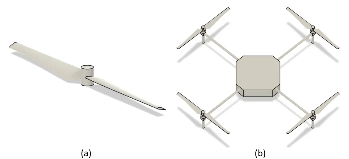
Autodesk Fusion, Ansys Workbench 2025 R1 Student version [16] are used in this study . A simplified quadcopter drone and propeller model was designed using Autodesk Fusion, as illustrated in Figure 1a,b.
 |
 |
|
(c) |
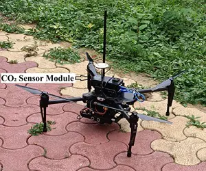
Figure 1. UAV structure: (a) Propeller of the drone, (b) Quadcopter Design, (c) Actual Quadcopter.
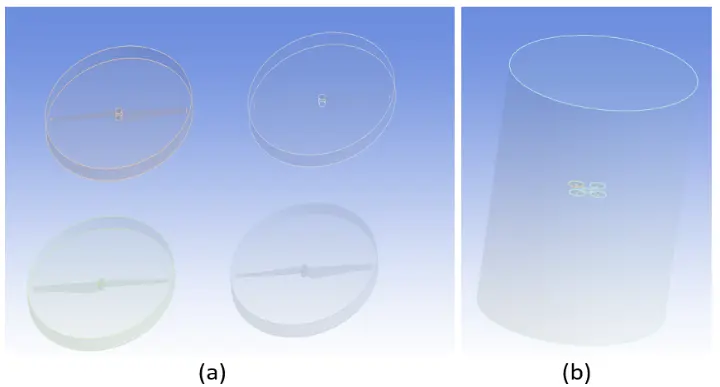
The quadcopter measures 27 mm in height, with a diagonal rotor-to-rotor distance of 212.132 mm and 100-mm-long rotor blades. The model was imported into Ansys Workbench 2025 R1 Student version, as shown in Figure 2a,b, with a cylindrical computational domain of 2 m in height and 0.5 m in radius.
A decent mesh was generated with a good amount of total number of elements, and nodes were formed in the mesh for examination. The aerodynamic layout of the four-rotor system studied in this paper is shown in Figure 3b. The angle between neighbouring rotors/propellers is 90°. The centre coordinates of the four rotors/propellers are s1cw (75,75,0) mm, s2ccw (75,−75,0) mm, s3cw (−75,−75,0) mm, s4ccw (−75,75,0) mm.
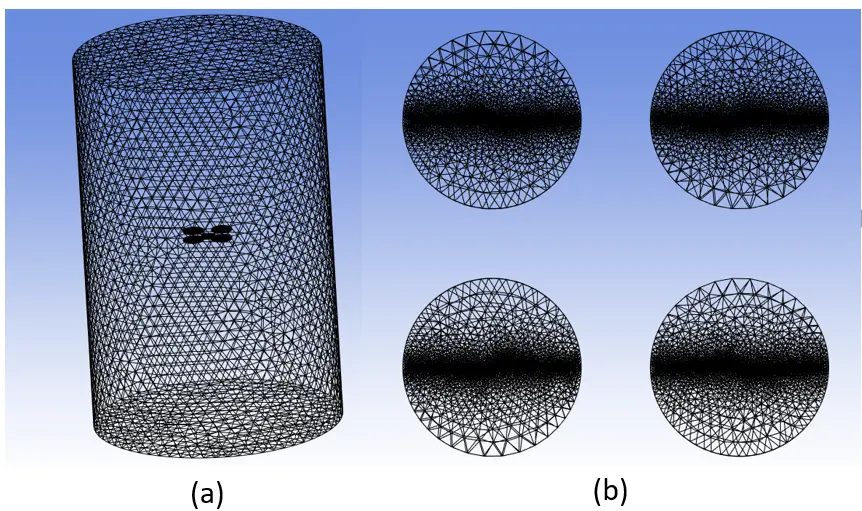
Figure 3. Diagram of grid division in the computational domain: (a) Grid division of static domains and (b) Grid division of rotating domains.
To ensure the accuracy of the numerical simulation, the computational domain is divided into a static domain and four rotating domains, including the rotor, as shown in Figure 2. The structure is named “Outer Cylinder”, and the rotating domains are named clockwise and anticlockwise as s1cw to s4ccw. Then we moved to the next step. Determining a dimensionless value y+15 to enter the height of the mesh’s initial layer is a prerequisite for performing boundary mesh division. This can be expressed as follows:
|
```latex{\mathrm{y}}^{+}=\frac{{\mathrm{u}}^{\mathrm{*}}{\mathrm{y}}_{1}}{\mathrm{\nu }}``` |
In the equation, y1 is the distance from the wall to the first mesh node; u* represents the friction velocity near the wall; and v is the kinematic viscosity of air.
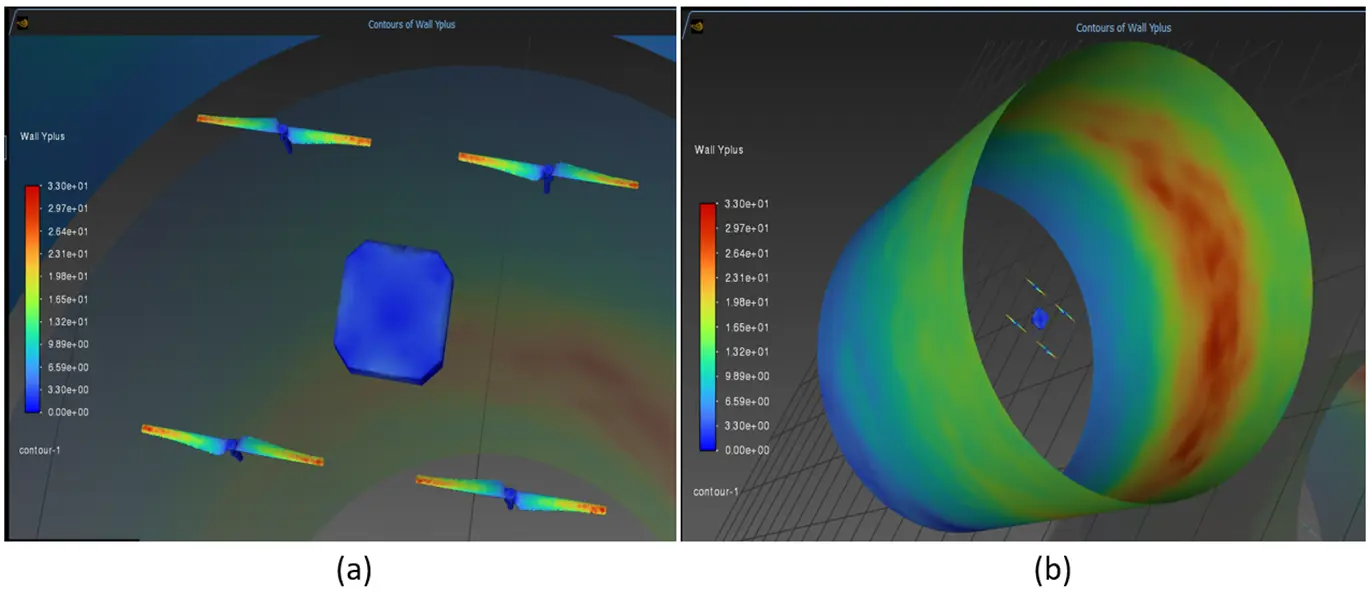
Drone rotors/propellers rotate at fast speeds, which causes significant turbulence in the wind. The simulation used in this study uses a high Reynolds number turbulence model, which well reflects the essential features of the turbulent flow. Figure 4 displays the measured y+ values, which range from 30 to 300 based on accurate numerical simulations. For turbulence models with a high Reynolds number, this range corresponds to the suggested application criteria. Consequently, it can be said that the mesh division approach used in this investigation is appropriate and able to faithfully depict the intense turbulent flow produced by drone rotors and propellers.
The governing fluid dynamics equations are discretized in the numerical simulation using the Finite Volume Method (FVM). Each of the four spinning domains is modelled as a no-slip moving wall because our study only looks at the drone’s hovering condition. The inlet and outlet bounds are specified as velocity inlet (0.2 m/s) and pressure outlet conditions, respectively. Turbulence intensity and viscosity ratio boundary settings are used to specify turbulence; in this case, a 5% turbulence intensity and a 10% viscosity ratio were used. With neighbouring rotors spinning in opposing directions, the rotation axis and direction are set to correspond with the actual configuration. Six rotating speed conditions—1000, 2000, 3000, 4000, 5000, and 6000 rpm—are used to execute the simulations. When setting up the solver, this study chose a pressure-based, absolute velocity, and transient mode, which will help simulate time-dependent fluid flow. To account for the effects of gravity in the simulation, gravitational acceleration was simultaneously adjusted to a value of −9.81 m/s2, directed vertically downward.
Approximately 4000 iterations were required to reach convergence in a steady-state calculation. After that, the generated flow fields are taken out for in-depth examination. Given its extensive use and recognition as one of the most widely used turbulence models for engineering computations with high Reynolds numbers, this study selected the SST k-ω model for the viscous model.
3. Results and Discussion
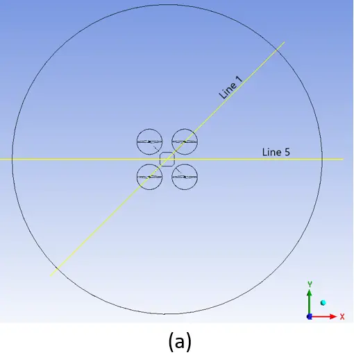
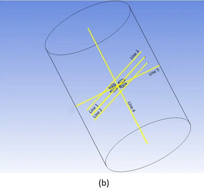
In the simulation, 5 locations were tested for the airflow line velocity as depicted in Figure 5a,b. After solving the calculations, the data are imported into CFD Post for post-processing. As shown in Figure 5, Five-line segments are set in the location. Line 1 Location (0.5,0.5,0) (−0.5,−0.5,0) m. Line 2 Location (0.5,0.5,−0.1) (−0.5,−0.5,−0.1) m. Line 3 Location (0.5,0.5,0.1) (−0.5,−0.5,0.1) m. Line 4 Location (0,0,1) (0,0,−1) m. Line 5 Location (0.75,0,0) (−0.75,0,0) m.
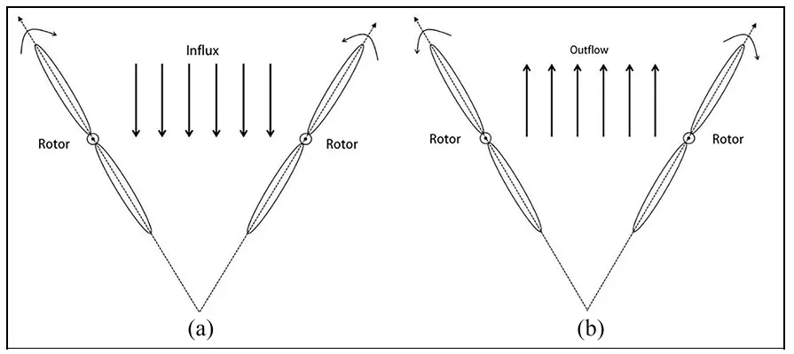
Inflow and Outflow, as shown in Figure 6 below when both adjacent rotors/propellers guide the gas into the inner circle, the motion state is called inflow. However, if the guided gas flows toward the outer circle, the motion state is referred to as outflow, as shown in the figure below.
Distribution of Airflow Velocity Along Different Lines
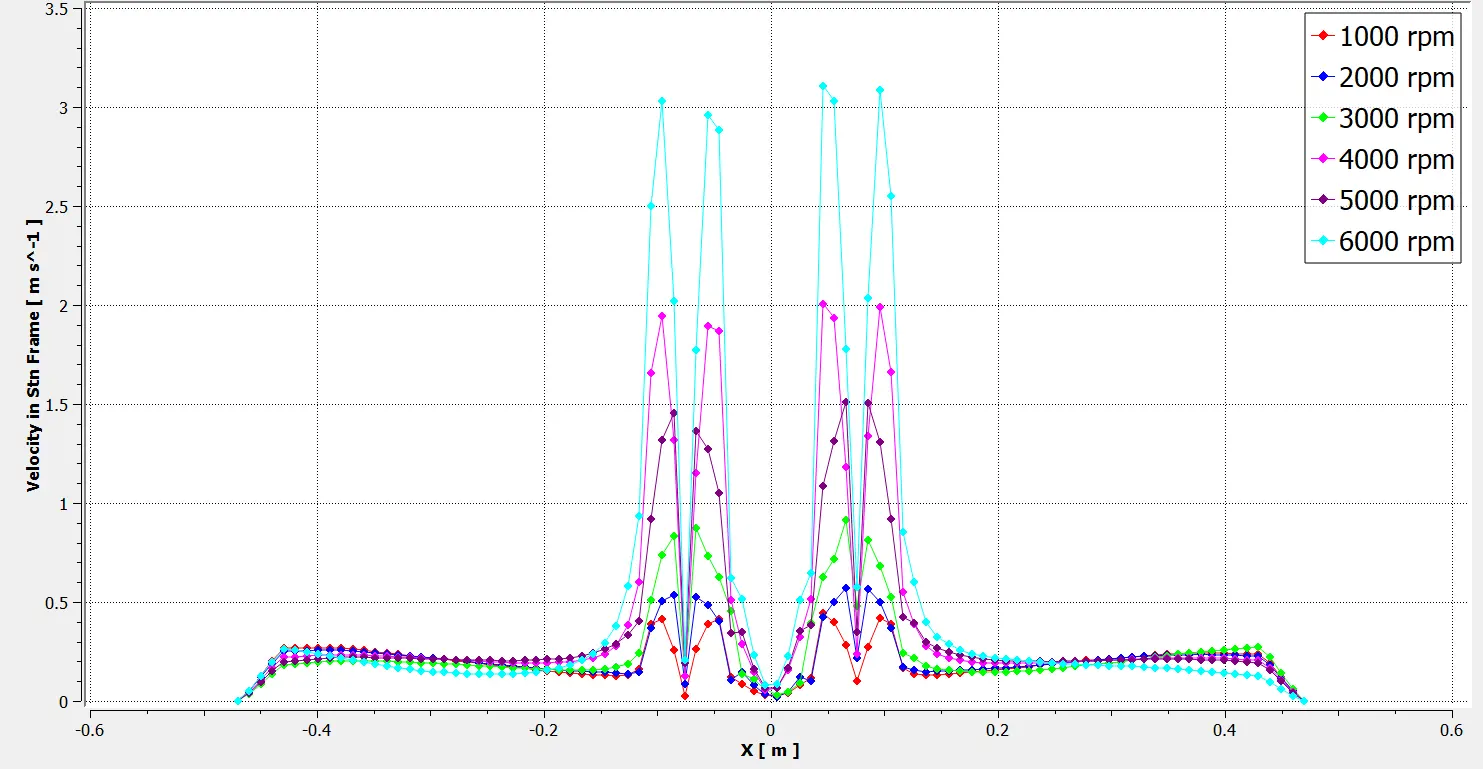
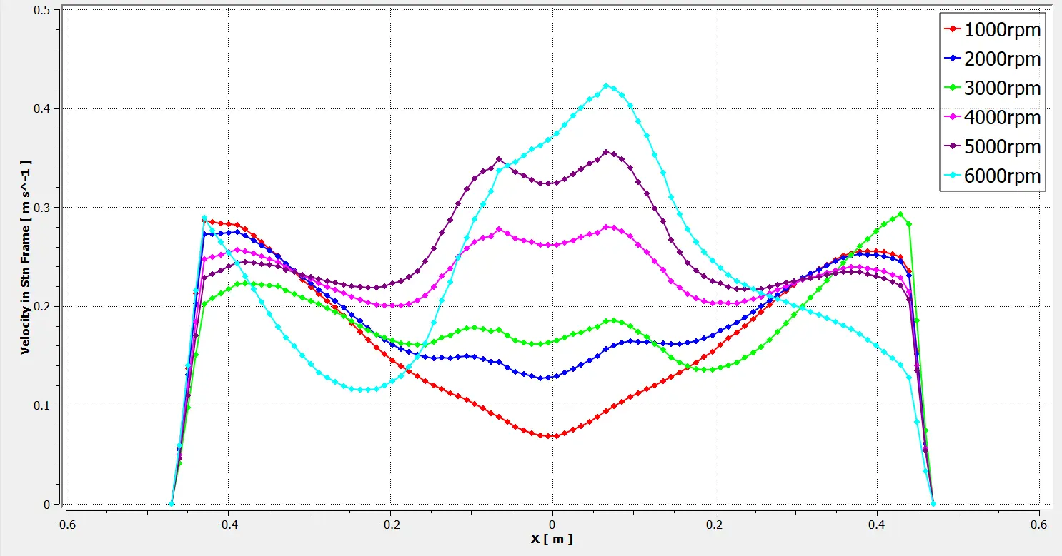
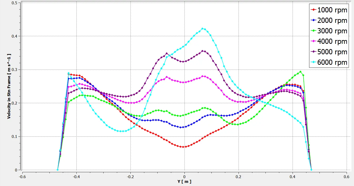
Airflow velocity along Line 1: In Figure 7a,b, the airflow velocity along both the X-axis and Y-axis is nearly symmetric about X = 0 m and Y = 0 m, respectively. Four distinct velocity peaks are observed at the tips of each rotor along the corresponding axis. As RPM increases, the rotor pushes more air downward—a stronger downwash field forms. This is reflected in the increasing central velocity peaks at higher RPMs. For instance, at a rotor speed of 6000 r/min, the velocities from left to right are 3.02, 2.90, 3.10, and 3.12 m/s, respectively. The airflow velocity is 0 m/s at both the central plate and the rotor hub. As the distance from the UAV’s origin increases, the airflow velocities on either side gradually decrease, eventually tending toward 0.5 m/s. It shows four distinct peaks aligned with rotor tips, confirming strong localized downwash right under each propeller. Velocity falls to near zero at the centre hub and outward, reinforcing that the core body area experiences minimal disturbance. Implies sensors should not be placed beneath or near rotor arcs.
 (a) 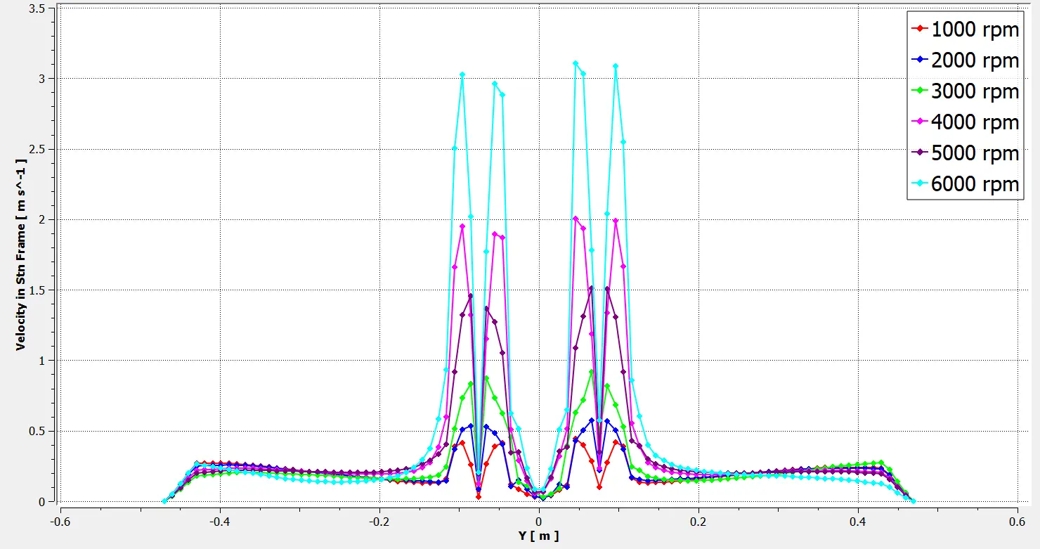 (b) |
Figure 7. Distribution of airflow velocity on line 1 at various rotational speeds (a) on X Axis, (b)Y Axis.
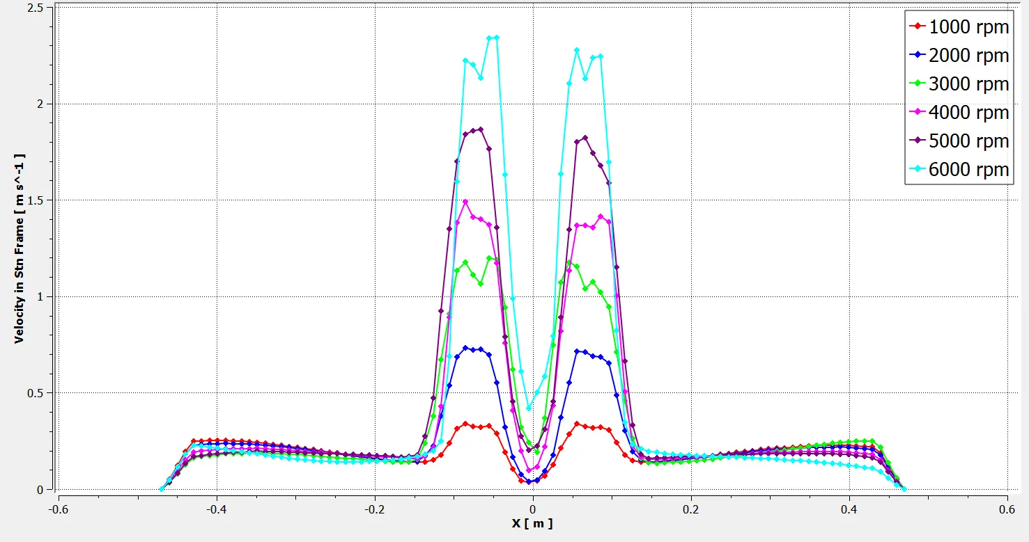
Airflow velocity along Line 2: The variation of airflow velocity on Line 2 is shown in Figure 8a,b. It exhibits four relatively symmetrical peaks below the tip of the rotor. Due to mutual interference of downwash airflow, the middle region between the peaks also experiences higher airflow velocity. The velocities on both sides gradually decrease toward 0 m/s as the distance from the UAV increases. Similar multi-peak structure but with higher disturbance between rotors due to interacting downwash streams. The entire line sits in a higher-energy flow zone, meaning even mid-plane below the frame is aerodynamically noisy. Implies placing sensors below the drone risks significant flow contamination.
 (a) 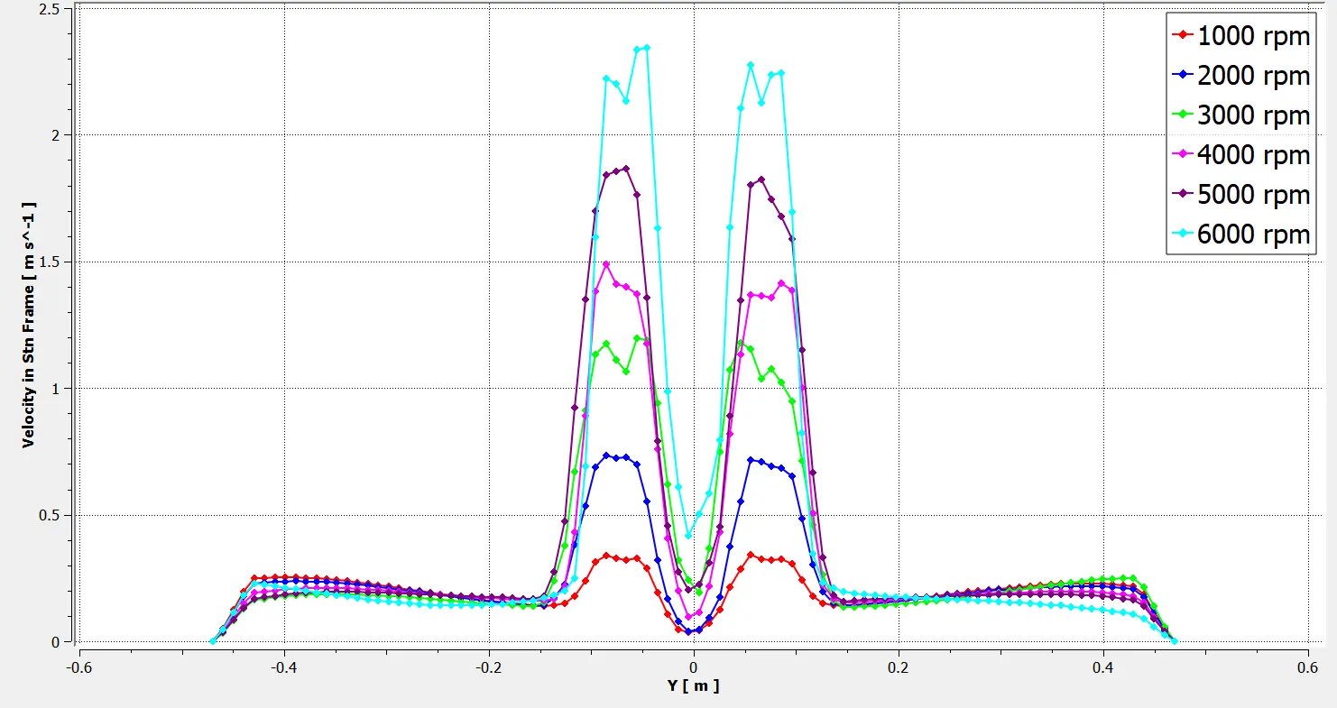 (b) |
Figure 8. Distribution of airflow velocity on line 2 at various rotational speeds. (a) on X Axis, (b)Y Axis.
It shows reduced overall velocities and weaker peak structures above the drone compared to below. Higher RPM cases only begin to show noticeable interaction, but are still lower than the underside. Indicates a cleaner sampling region just above the fuselage.
Airflow velocity along Line 3: The variation of airflow velocity on Line 3 is shown in Figure 9a,b. Two peaks near the ends (~±0.45 m) correspond to propeller tip influence or strong downwash regions. A central velocity jump for higher RPM cases (5000–6000 rpm), indicating intensified interaction of downwash flows from opposing rotors/propellers. At low RPM (1000–2000), the centre region shows a clear velocity trough (~0.12–0.18 m/s), suggesting weak interaction and greater separation between the rotor flows. The curves remain almost symmetric about X = 0, indicating balanced rotor performance. We can see that the airflow velocity above the drone frame (Line 3) is less than at the same height below the drone frame (Line 2).
 |
|
(a) |
 |
|
(b) |
Figure 9. Distribution of airflow velocity on line 3 at various rotational speeds. (a) on X Axis, (b)Y Axis.
Airflow velocity along Line 4: Line 4 coincides with the Z-axis. By analysing the changes in velocity along Line 4, the distribution pattern of airflow velocity in the Z-axis direction is obtained. In Figure 10, we can observe that at a height of 0.5 m above the fuselage, the airflow velocity is close to 0 m/s. The airflow velocity is highest near the rotor, reaching a maximum of 1.75 m/s below the drone frame and 0.4 m/s above the drone frame. The airflow velocity above the fuselage is noticeably lower than that below the fuselage. Airflow drops rapidly to near-zero above the drone but intensifies sharply below the rotors. It demonstrates asymmetric flow: calm stagnation dome above, expanding turbulent jet downward, and confirms that vertical upward mounting is optimal over downward or belly-side placement.
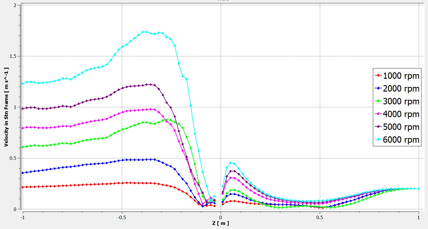
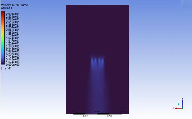
Referring to the X–O–Z plane velocity profile cloud map in Figure 11, due to the disturbance of the rotor and the influence of atmospheric pressure, there is a local turbulent region below the fuselage. Therefore, in Figure 10 shows that the airflow velocity increases again after a decrease in the negative z-direction. The overall trend along line 4 is that the airflow velocity decreases with increasing vertical distance above the drone frame, and the airflow velocity increases with negative Z vertical distance. The airflow velocity is very low close to the aircraft’s solid wall surface. The airflow velocity above the fuselage will drop to 0 m/s more quickly than the airflow velocity at the same distance below the fuselage because the former is substantially smaller.
Airflow velocity along Line 5: The line 5 is the X-axis passing through the origin of the drone frame. The X–O–Y cross-section at Z = 0 m is displayed in Figure 12. It is evident from the image that the four peaks of the airflow velocity on Line 5 are situated at the four tangent circles of the hub’s outer boundary and the rotor’s rotating domain. The airflow velocity on both sides trends toward 0 m/s as the horizontal distance from the drone rises, whereas the hub region’s velocity is 0 m/s.
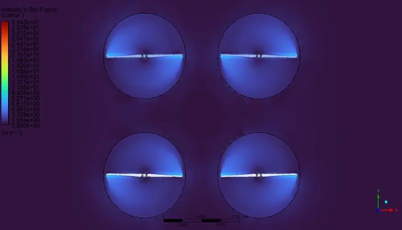
As seen in Figure 13, the airflow velocity along Line 5 is symmetric about Z = 0 m. The velocity in the X-axis’s positive direction is substantially less than the velocity in its negative direction. The maximum value on the negative half-axis is 0.59 m/s, while the maximum value on the positive half-axis is just 0.57 m/s, using 6000 r/min as an example.
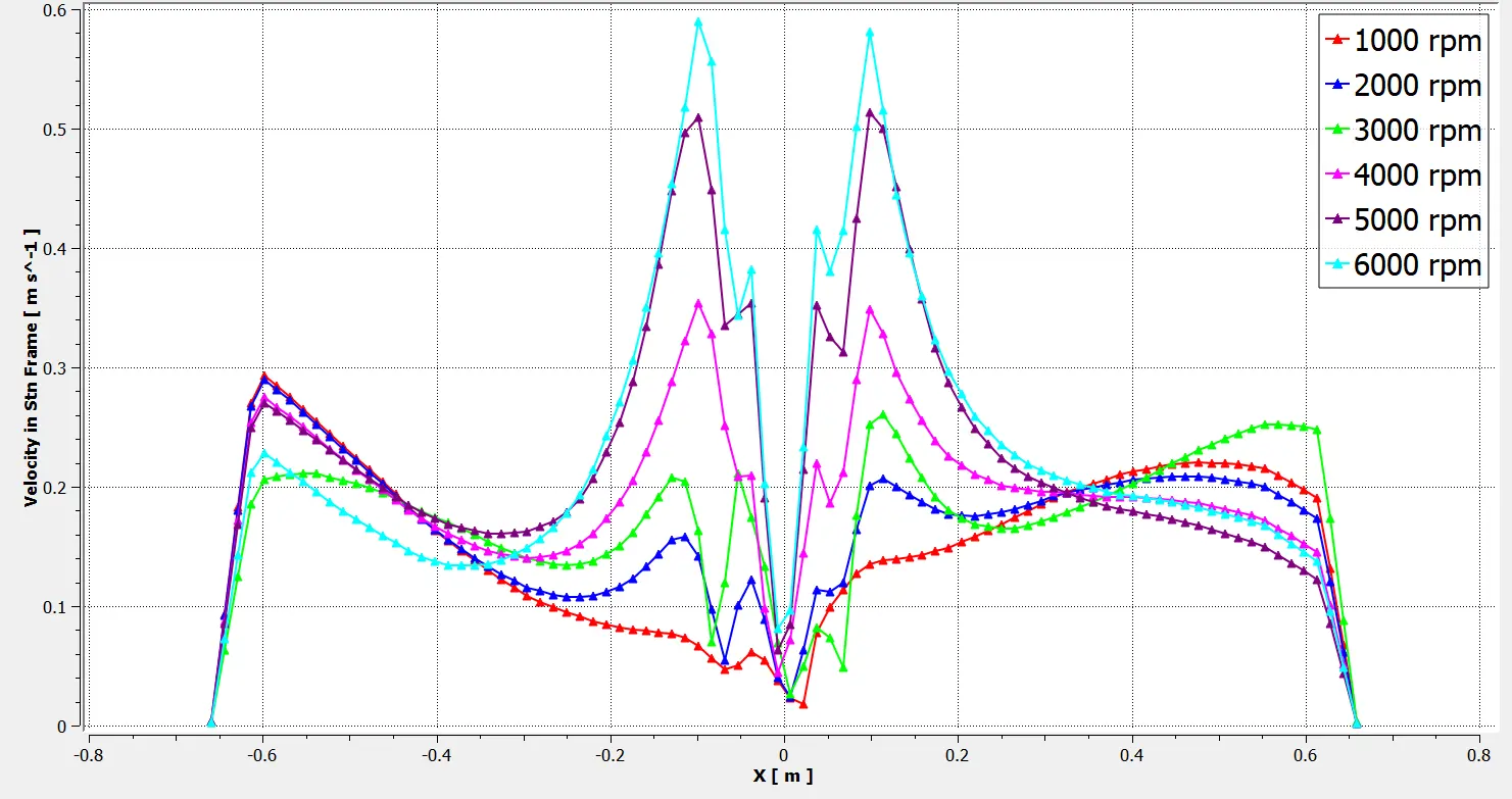
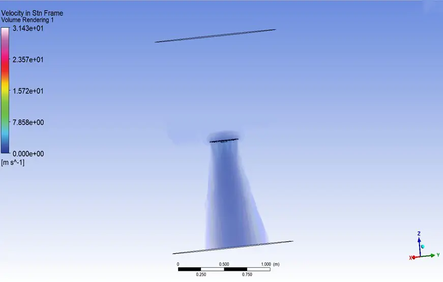
Figure 14 below is the volume rendering plot of the drone, which clearly shows the region of disturbance both above and below the drone. We can observe that the disturbance area is more below the drone than above. Turbulent cloud dominates the lower hemisphere; the upper region remains visibly calmer. Turbulence footprint expands with RPM and extends further downward than laterally. Visually reinforces the need to avoid underside placement.
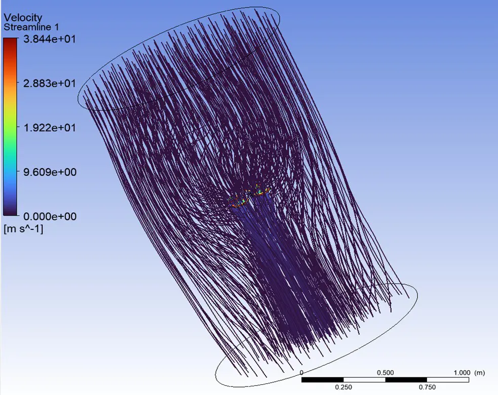
In Figure 15, the streamlines show airflow created by the quadcopter’s rotors/propellers, with flow entering from the top and moving downward from the force of the rotors/propellers. The velocity range (0 to 38 m/s) near the rotor plane (top and centre) suggests significant acceleration, while velocities decrease toward the cylinder walls and bottom. It shows a coherent downward jet forming from converging rotor flows and accelerating toward the lower domain. Flow lines diverge outward at lower heights, indicating plume dilution and strong entrainment. It demonstrates why lightweight gases are most error-prone if sampled below.
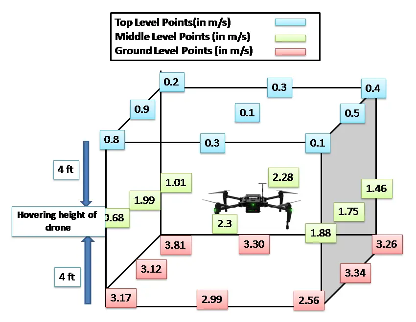
Validation of the results was performed using experimental data. The wind speed during the hovering mode, measured at distances beyond 4 feet, was plotted in three dimensions.It is depicted in Figure 16. Contour lines were generated to analyze the regions of airflow disturbance. The results indicate that the disturbed airflow region is predominantly located above the ground level.
4. Conclusions
This study shows the impact of rotor rotation on the surrounding airflow velocity by simulating the flow field of a quadcopter. The contour plots and line graphs summarize the findings. Using CFD, simulation and result analysis were done on how the surrounding wind speed changed following the drone’s rotor revolution. With the exception of the airflow velocity at the centre plate area, which is 0 m/s, the distribution patterns of airflow velocity in the X-axis and Y-axis directions within the same horizontal plane at a specific height show that the velocity decreases toward 0 m/s as the distance from the drone increases above. As a result, the sensor can be positioned at a suitable distance from the drone’s rotor (approx. 0.3 m horizontally away from the drone’s central plate) or in the middle plate area (approx. 0.4 m above the drone above plate).
This is how air is forced downward and spread outward by the rotor wash effect. Dense, convergent streamlines in the centre indicate strong downward airflow from the propellers. Looping or chaotic patterns may suggest turbulence, which often occurs in rotor-induced flows, especially near the rotor tips. Similar research can be conducted for larger drones to improve the placement of the sensor payload at a comparable height, as this study was conducted on a smaller drone. We need an area with the least amount of disruption when the drone is flying to install our sensors. Our CFD study strongly suggests that sensors should be positioned either horizontally away from the drone or on top side during environmental analysis.
Acknowledgements
G.K. and P.G. thank to Devicha Centre for Climate Change for travel and other support during study.
Author Contributions
Conceptualization: P.K., G.K.; Methodology, P.K.; Software: G.K., P.G.; Validation: A.M., P.K.; Formal Analysis: P.G.; Original Draft Preparation: P.K. & G.K.; Review & Editing: P.G. & A.M.
Ethics Statement
Not Applicable.
Informed Consent Statement
Not Applicable.
Data Availability Statement
The data is available with CSIR-NEERI.
Funding
This research received no external funding.
Declaration of Competing Interest
The authors declare that they have no known competing financial interests or personal relationships that could have appeared to influence the work reported in this paper.
References
-
Jońca J, Pawnuk M, Bezyk Y, Arsen A, Sówka I. Drone-Assisted Monitoring of Atmospheric Pollution—A Comprehensive Review. Sustainability 2022, 14, 11516. DOI:10.3390/su141811516 [Google Scholar]
-
Li XB, Wang DS, Lu QC, Peng ZR, Wang ZY. Investigating vertical distribution patterns of lower tropospheric PM2.5 using unmanned aerial vehicle measurements. Atmos. Environ. 2018, 173, 62–71. DOI:10.1016/j.atmosenv.2017.11.009 [Google Scholar]
-
Osei-Ntansah K, Reliford A, Smith ST. Design and Implementation of 3D Printed Sensor Mounts for sUAS-Based Atmospheric Research. In Proceedings of the AIAA SCITECH 2025 Forum, Orlando, FL, USA, 6–10 January 2025. [Google Scholar]
-
Li S. Wildfire early warning system based on wireless sensors and unmanned aerial vehicle. J. Unmanned Veh. Syst. 2018, 7, 76–91. DOI:10.1139/juvs-2018-0022 [Google Scholar]
-
Ventura Diaz P, Yoon S. High-fidelity simulations of a quadrotor vehicle for urban air mobility. In Proceedings of the AIAA SciTech 2022 Forum, San Diego, CA, USA, 3–7 January 2022. p. 0152. DOI:10.2514/6.2022-0152 [Google Scholar]
-
Ilyas M, Noack BR, Hu G, Xiong H, Gao N, Khan A, et al. Drone anemometry of atmospheric winds—A review. Phys. Fluids 2025, 37, 061302. DOI:10.1063/5.0259355 [Google Scholar]
-
Christodoulou K, Vozinidis M, Karanatsios A, Karipidis E, Katsanevakis F, Vlahostergios Z. Aerodynamic Analysis of a Quadcopter Drone Propeller with the Use of Computational Fluid Dynamics. Chem. Eng. Trans. 2019, 76, 181–186. DOI:10.3303/CET1976031 [Google Scholar]
-
Rangan S, Shanmugam Y, Valluvan G, Prakash T. A customized drone for ocean and atmospheric measurements and its performances. Marit. Technol. Res. 2024, 6, 267638. DOI:10.33175/mtr.2024.267638 [Google Scholar]
-
Yaakub MF, Wahab AA, Abdullah A, Mohd NN, Shamsuddin SS. Aerodynamic prediction of helicopter rotor in forward flight using blade element theory. J. Mech. Eng. Sci. 2017, 11, 2711–2722. [Google Scholar]
-
Kokate P, Middey A, Sadistap S. Drone-Aided Particulate Monitoring System for Industrial Complex to Analyze the Dust Suppressing Capacity. J. Appl. Eng. Sci. 2023, 13, 237–242, DOI:10.2478/jaes-2023-0030 [Google Scholar]
-
Ventura Diaz P, Yoon S. High-Fidelity Computational Aerodynamics of Multi-Rotor Unmanned Aerial Vehicles. In Proceedings of the 2018 AIAA Aerospace Sciences Meeting, Kissimmee, FL, USA, 8–12 January 2018. DOI:10.2514/6.2018-1266 [Google Scholar]
-
Shamsudin SS, Madzni MZ. Aerodynamic Analysis of Quadrotor UAV Propeller using Computational Fluid Dynamic. J. Complex Flow 2021, 3, 28–32. [Google Scholar]
-
Arafat M, Ishak IA, Mohd Maruai N, Muhammad Razif MR, Mohd Sakri F, Anugraha RA. CFD Assessment for Small UAV Propeller Aerodynamics. CFD Lett. 2024, 17, 81–92. DOI:10.37934/cfdl.17.6.8192 [Google Scholar]
-
Umirzakova S, Muksimova S, Shavkatovich Buriboev A, Primova H, Choi AJ. A Unified Transformer Model for Simultaneous Cotton Boll Detection, Pest Damage Segmentation, and Phenological Stage Classification from UAV Imagery. Drones 2025, 9, 555. DOI:10.3390/drones9080555 [Google Scholar]
-
Russell S, Carl R, Martin K. Comprehensive Analysis Modeling of Small-Scale UAS Rotors - NASA Technical Reports Server (NTRS). Available online: https://ntrs.nasa.gov/citations/20170011320 (accessed on 26 January 2026)
-
İnan AT, Çetin B. CFD Analysis of Aerodynamic Characteristics in a Square-Shaped Swarm Formation of Four Quadcopter UAVs. Appl. Sci. 2024, 14, 6820. DOI:10.3390/app14156820 [Google Scholar]