
Normalized Source-Storage-Load Flexibility-Loss Indicators for Day-Ahead Scheduling of Renewable Virtual Power Plants

Normalized Source-Storage-Load Flexibility-Loss Indicators for Day-Ahead Scheduling of Renewable Virtual Power Plants
Lai Jiang 1 Yufeng Guo 1,* Rui Bao 1 Qi Wang 2 Wei Xu 1 Yihang Ouyang 1 Yuxin Jiang 1 Lichaozheng Qin 1
Received: 25 May 2026 Revised: 03 July 2026 Accepted: 20 July 2026 Published: 30 July 2026

© 2026 The authors. This is an open access article under the Creative Commons Attribution 4.0 International License (https://creativecommons.org/licenses/by/4.0/).
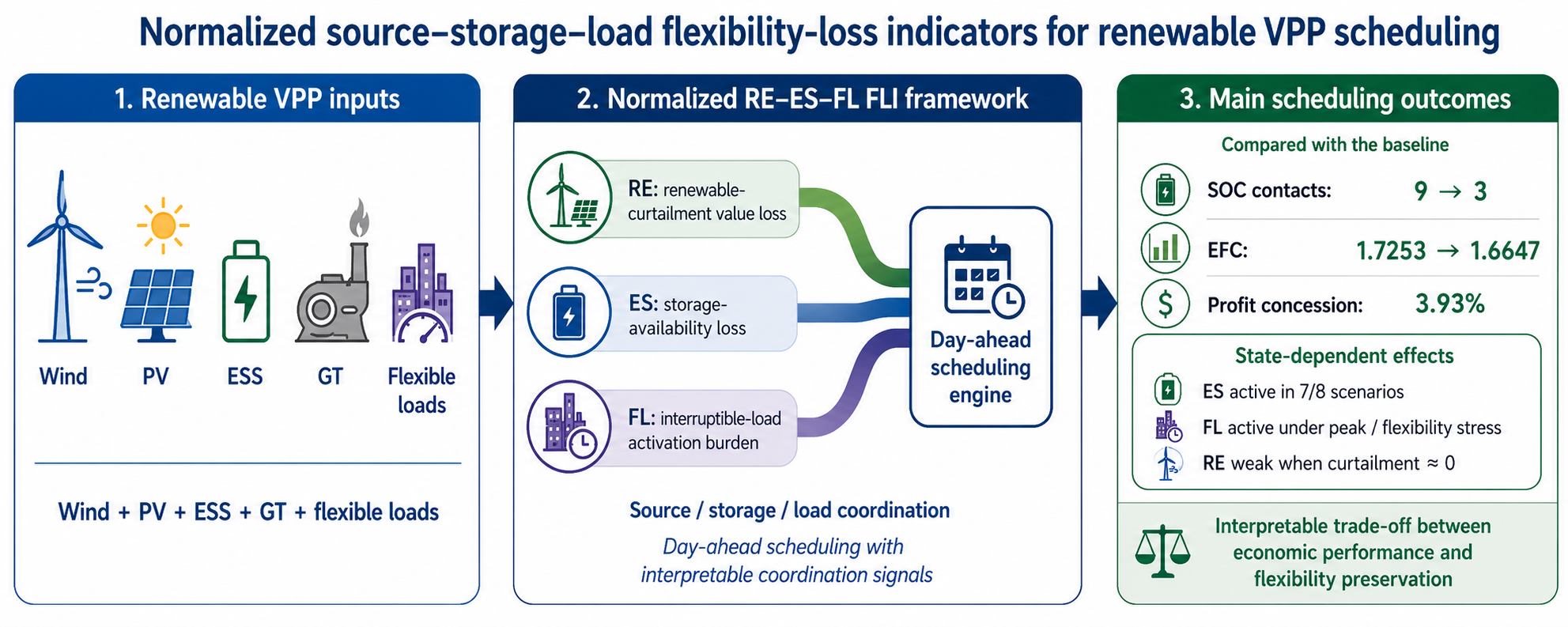
Graphical Abstract
1. Introduction
Smart energy systems are increasingly required to coordinate renewable generation, flexible demand, and distributed operating resources under a common scheduling framework. High renewable penetration increases the importance of dispatch decisions that preserve operating flexibility while maintaining economic performance [1]. Forecasting studies further show that renewable and demand trajectories are becoming more observable, but forecast information must still be translated into dispatchable coordination signals [2,3].
A renewable-based virtual power plant (VPP) offers one practical aggregation structure for this task. Through a VPP operator, wind power, photovoltaic (PV) generation, gas turbines (GTs), energy storage systems (ESSs), interruptible loads (ILs), and shiftable loads (SLs) can be scheduled as an integrated portfolio. Renewable VPP bidding studies have shown that wind, solar, and dispatchable loads can be jointly coordinated in market-facing operation [4]. Multi-aggregator VPP studies further indicate that aggregation structure affects the feasible dispatch space and resource responsibilities [5].
A large body of VPP research addresses uncertainty through stochastic, robust, and interval formulations. Stochastic robust optimization has been used to coordinate VPPs with multiple uncertain resources [6]. Robust scheduling and receding-horizon dispatch have also been developed for VPP service provision under uncertain operation [7]. Endogenous and exogenous uncertainty modeling further improves robust VPP schedules when uncertainty is affected by decisions [8]. Recent work on decomposed stochastic programming and decision-dependent robust operating-region methods extends this line of work to multi-energy and multistage systems [9,10]. Risk-preference and interval bidding studies further consider how uncertainty affects market-facing VPP schedules [11,12]. Decision-driven robust multi-market scheduling and probabilistic-constraint surrogates also address uncertainty in market-coupled VPP operation [13,14].
Another stream of studies focuses on market participation, reserve provision, and multi-service operation. Joint energy-reserve-carbon scheduling broadens the VPP objective beyond energy arbitrage alone [15]. Multi-market trading models consider energy, ancillary-service, and carbon-market interactions [16]. Market-pricing and reserve mechanisms introduce additional settlement and feasibility considerations for dispatch models [17,18]. VPP aggregation models for inertia and primary frequency response further show that participation in ancillary services can reshape the role of distributed resources [19]. Energy-frequency regulation studies extend this perspective to frequency-service scheduling under uncertainty [20]. VPP assembly, profit allocation, and multi-market participation studies further highlight the institutional aspects of VPP coordination [21,22]. Convex hull pricing work also shows that nonconvex market settlement can affect dispatch incentives [23].
Demand response and multi-entity coordination provide complementary sources of operational flexibility. Incentive-based demand-response programs can adjust VPP operation by modifying flexible demand profiles [24,25]. VPP scheduling with demand-response resources has also been studied in electricity-market environments under uncertainty [26]. Game-based and multi-entity VPP models show that coordination rules affect both dispatch outcomes and participant interactions [5,27]. Coordinated operation with multiple DER aggregators further shows that participant-level representation can affect VPP dispatch responsibilities [28]. These studies confirm that load flexibility is not merely a passive demand correction, but a controllable resource that changes the scheduling solution.
Flexible operating regions and scalarized multi-term formulations provide useful ways to describe feasible operation and trade-offs. Flexible-operation-region studies characterize the boundary of available VPP flexibility [29]. Adaptable multi-objective optimization methods show that weighted scalar formulations can represent different scheduling preferences [30]. Multi-timescale scheduling also links load flexibility to storage degradation considerations [31]. Risk-based and mobile-storage multi-objective VPP studies further illustrate how scalarized preferences can change economic and operational trade-offs [32,33]. However, such formulations often report the final dispatch and objective value without explicitly diagnosing which physical flexibility channel has been consumed. As a result, renewable accommodation, storage preservation, and load-side activation may remain difficult to separate in the interpretation of one day-ahead schedule.
The present work, therefore, targets a narrower but important gap: transparent diagnosis of source-storage-load flexibility consumption within a deterministic day-ahead VPP schedule. The paper does not claim that curtailment, SOC-related, or flexible-load penalty terms are new in isolation. Instead, it organizes these effects into a normalized source-storage-load flexibility-loss-indicator (FLI) framework with explicit channel weights, reference scales fixed within each comparative setting, and channel-ablation diagnostics. The term flexibility-loss indicator is used deliberately because the proposed quantities are engineering proxies for selected implicit flexibility losses, not strict market-settled opportunity costs or a complete uncertainty-risk measure.
The proposed framework separates three physical channels. The renewable-side indicator describes curtailment-related value loss, the storage-side indicator describes insufficient storage availability and boundary pressure, and the flexible-load-side indicator describes interruptible-load activation burden. The three channels are normalized before entering the scalarized objective, which reduces the risk that one unscaled term dominates the optimization only because of its numerical magnitude. This structure also allows the effect of each channel to be tested through weight sensitivity and Full-versus-No-channel ablation rather than inferred from a single objective value.
The contributions of this study are threefold. First, a renewable VPP scheduling model is formulated in which dispatchable wind and PV outputs enter both the power-balance equation and the renewable-utilization metric and constraint. Second, normalized RE, ES, and FL indicators are constructed under a unified scalar objective to represent renewable-curtailment value loss, storage availability loss, and interruptible-load activation burden. Third, a main-case comparison, a weight-sensitivity analysis, a channel ablation, and representative operating and stress-test scenarios are used to diagnose the state-dependent effects and practical boundaries of the proposed framework.
2. Methodology
The proposed framework coordinates short-term economic performance, internal operating burden, renewable accommodation, and flexibility preservation within a day-ahead virtual power plant (VPP) scheduling problem. Three normalized flexibility-loss indicators (FLIs) are introduced for renewable generation, energy storage, and interruptible load. These indicators are engineering proxies for selected dispatch-relevant flexibility losses rather than market-settled opportunity costs or comprehensive uncertainty-risk measures.
The scheduling horizon consists of $$T = 24$$ hourly periods, with $$\Delta t = 1\,\text{h}$$. Unless otherwise stated, all time-dependent constraints apply to $$t \in \{1,\dots,T\}$$.
2.1. Scalarized Multi-Term VPP Dispatch Model
The day-ahead VPP scheduling problem is formulated as a scalar mixed-integer quadratic programming (MIQP) problem. The objective combines the net operating-cost term, an internal operating-coordination term, and the normalized FLI term:
where $$C_{\text{tot}}$$ is the net operating-cost expression, $$C_{\text{coord}}$$ represents the controllable internal operating burden, and $$\Phi_{\text{FLI}}$$ is the normalized source–storage–load FLI contribution. The switches $$d_o$$ and $$d_{\text{FLI}}$$ determine whether the coordination and FLI terms are enabled.
The outer coefficients are fixed throughout the comparative analysis as
These coefficients are not claimed to be theoretically optimal. The adopted setting retains the economic term as the dominant component while assigning limited weights to internal operational coordination and the preservation of flexibility. The sensitivity analysis changes only the inner RE, ES, and FL channel weights defined in Section 2.2, while the outer coefficients remain unchanged.
All three comparative models use the same physical constraints and renewable-utilization requirement. Their objective structures are summarized in Table 1.
Table 1. Objective-term definitions of the comparative models.
|
Model |
d_o |
d_FLI |
Economic Term |
Coordination Term |
FLI Term |
|---|---|---|---|---|---|
|
Baseline model |
0 |
0 |
Included |
Not included |
Not included |
|
Scalarized multi-term reference model |
1 |
0 |
Included |
Included |
Not included |
|
Proposed FLI model |
1 |
1 |
Included |
Included |
Included |
2.1.1. Economic Term
The economic performance reported in the case study is the VPP net operating profit:
The complete net operating-cost expression is
where $$C_{\text{grid}}$$ is the signed grid-transaction cost, $$C_{\text{GT}}^{\text{fix}}$$ is the fixed GT fleet charge used in the implemented model, $$C_{\text{op}}$$ is the controllable operating-cost expression, $$C_{\text{ESS}}^{\text{fix}}$$ is the fixed ESS maintenance cost, and $$R_{\text{retail}}$$ is the retail-load revenue term used consistently in all comparative cases.
The fixed GT fleet charge is expressed as
where $$N_{\text{GT}}$$ is the number of GT units and $$c_{\text{GT}}^{\text{fix}}$$ is the fixed charge assigned to each unit. This term is constant within each comparative case and does not represent an endogenous start-up or shut-down payment.
The grid-transaction cost is evaluated using a signed grid-exchange variable:
where $$\rho_{t}^{\text{b}}$$ and $$\rho_{t}^{\text{s}}$$ are the grid purchase and selling prices, respectively. A positive $$P_{\text{grid},t}$$ denotes electricity purchase from the grid, whereas a negative value denotes grid export. During export, the second term in Equation (6) is negative and therefore reduces the net operating cost.
The signed representation avoids treating the purchase and sale of electricity as two independent, simultaneous decisions in the deterministic single-bus formulation. No explicit grid-export capacity limit is imposed in the present model.
2.1.2. Internal Operating-Coordination Term
The controllable non-FLI operating cost is
where $$C_{\text{GT}}^{\text{gen}}$$ is the GT generation cost; $$C_{\text{GT}}^{\text{up}}$$ and $$C_{\text{GT}}^{\text{down}}$$ are the fleet-level upward and downward reserve costs; $$C_{\text{W}}^{\text{dev}}$$ and $$C_{\text{PV}}^{\text{dev}}$$ are wind and PV forecast-deviation penalties; $$C_{\text{ESS}}^{\text{op}}$$ is the variable ESS operating cost; and $$C_{\text{FL}}^{\text{comp}}$$ is the flexible-load compensation cost.
The internal coordination term is
The coordination term deliberately reweights the controllable operating burden that is already included in the economic accounting. It is therefore a scalarization device rather than an additional physical payment charged twice to the VPP. Its role is to express a preference for schedules with lower internal operating burden while retaining net operating profit as the dominant consideration.
2.1.3. Renewable-Utilization Constraint
Renewable utilization is defined as the ratio between scheduled and available wind and PV energy:
where $$P_{\text{W},t}^{\text{av}}$$ and $$P_{\text{PV},t}^{\text{av}}$$ are the available wind and PV upper limits, while $$P_{\text{W},t}^{\text{sch}}$$ and $$P_{\text{PV},t}^{\text{sch}}$$ are dispatch variables.
The renewable-utilization requirement is
Renewable utilization is therefore imposed as a common constraint rather than treated as an additional scalar objective. The same threshold is applied to all three comparative models.
2.1.4. Gas-Turbine and Reserve Costs
The GT generation cost is represented using quadratic unit-level output-cost functions:
where $$P_{\text{GT},i,t}$$ is the output of GT unit $$i$$, and $$a_i$$,$$\,b_i$$, and $$c_i$$ are the corresponding cost coefficients.
The fleet-level reserve costs are
where $$R_{\text{GT},t}^{\text{up}}$$ and $$R_{\text{GT},t}^{\text{down}}$$ denote the total upward and downward reserve scheduled for the GT fleet.
The renewable forecast-deviation penalties are
where $$\varepsilon_{\text{W},t}$$ and $$\varepsilon_{\text{PV},t}$$ are the wind and PV forecast-deviation magnitudes, and $$\pi_{\text{W},t}$$ and $$\pi_{\text{PV},t}$$ are the corresponding penalty coefficients.
2.2. Normalized Flexibility-Loss Indicator Modeling
The FLI framework separates three operational channels:
-
renewable-curtailment value loss;
-
storage-availability loss;
-
interruptible-load activation burden.
The three indicators have different physical meanings and numerical scales. Fixed reference values are therefore used to normalize the indicators before they are combined.
The normalized FLI term is
where $$s_{\text{FLI}} = 2.5$$ is a fixed global scaling factor. The enabling parameters $$e_{\text{RE}}, e_{\text{ES}}, e_{\text{FL}} \in \{0,1\}$$ are used in the channel-ablation analysis.
The normalized channel coefficients are obtained from the specified channel-weight ratios:
The coefficients are normalized before the enabling parameters are applied. Therefore, disabling one channel does not redistribute its coefficient to the remaining channels. The equal ratio 1:1:1 is used as a mechanism-identification baseline rather than as a theoretically unique or optimized preference vector.
Within each sensitivity or ablation comparison, one set of reference scales is fixed and reused across all model variants. The reference scales are not recomputed separately for the Full, No-RE, No-ES, No-FL, and No-FLI cases.
2.2.1. Renewable-Side Indicator
The renewable-side indicator measures the value of available wind and PV power that is not scheduled:
The indicator becomes active only when renewable curtailment is physically or economically possible. When available renewable generation can be accommodated by load, storage, or grid export, $$L_{\text{RE}}$$ the approaches zero and have negligible marginal influence.
2.2.2. Storage-Side Indicator
The storage-side indicator represents insufficient SOC retention relative to future balancing requirements and operation close to the admissible SOC boundaries.
The forecast net load is
where $$P_{\text{D},t}^{\text{f}}$$ is the forecast baseline demand before demand-response adjustment.
The one-step-ahead upward net-load ramp requirement is
The renewable downside-deviation requirement is
where $$\Delta P_{\text{W},t}^{-}$$ and $$\Delta P_{\text{PV},t}^{-}$$ represent possible downward deviations of wind and PV output.
The dynamic SOC reference is constructed as
where
The term $$P_{\mathrm{ES}}^{\max}\Delta t$$ represents a baseline one-hour discharge capability retained in the storage state. The terms $$r_{t}^{+}$$ and $$\ u_{t}$$ add operating-state-dependent ramping and renewable-downside requirements. The clipping operator ensures that the reference remains within the allowable SOC range.
The SOC boundary-pressure term is
where $$\delta=0.10$$ is the adopted SOC boundary margin.
The storage-side indicator is
where $$\gamma_{B}=0.5$$ assigns a secondary weight to boundary-pressure avoidance relative to direct $$SOC$$-reference shortage. This coefficient is a modeling parameter rather than a fitted market price.
Unlike a static $$(1-SOC_{t})$$ expression, Equation (25) does not uniformly encourage high $$SOC$$. The preferred storage state changes with the forecast net-load ramp, renewable downside requirement, and current operating condition.
2.2.3. Interruptible-Load Indicator
The load-side indicator measures the incremental burden of activating interruptible load when its compensation requirement exceeds the value of electricity sold:
where $$\lambda_{\mathrm{IL},t}$$ is the interruptible-load compensation price, and $$\Delta P_{\mathrm{IL},t}$$ is the interrupted load.
The FL indicator is directly associated with interruptible-load activation. Changes in shiftable-load schedules are interpreted only as indirect system-level responses and are not used as direct evidence of the FL channel.
2.2.4. Reference Scales
The renewable-side reference scale is
the storage-side reference scale is
and the interruptible-load reference scale is
where epsilon > 0 is a small positive constant used to prevent division by zero.
2.3. Operational Constraints
2.3.1. Power-Balance Constraint
The optimized wind and PV dispatch variables enter the power-balance equation directly:
Here, $$P_{\mathrm{L},t}^{\mathrm{fix}}$$ is the non-flexible load, $$P_{\mathrm{IL},t}$$ is the actual interruptible load after curtailment, and $$P_{\mathrm{SL},t}$$ is the actual shiftable load after temporal redistribution.
The actual interruptible and shiftable loads are defined as
A positive $$\Delta P_{\mathrm{IL},t}$$ denotes curtailed interruptible demand. The shiftable-load adjustment $$\Delta P_{\mathrm{SL},t}$$ is signed: a positive value reduces demand in the current period, whereas a negative value increases demand because energy has been shifted into that period.
Substituting Equation (31) and Equation (32) into Equation (30) yields the equivalent demand-adjustment form used in the implementation, in which $$\Delta P_{\mathrm{IL},t}$$ and $$\Delta P_{\mathrm{SL},t}$$ appear on the supply side of the balance equation. Therefore, the physical-load representation and the implemented algebraic representation are mathematically equivalent.
Equation (30) ensures that changes in scheduled wind and PV output propagate to GT output, ESS operation, grid exchange, and flexible-load decisions.
2.3.2. Renewable Generation Constraints
The scheduled renewable outputs satisfy
Renewable curtailment is calculated consistently as
2.3.3. Gas-Turbine and Fleet-Level Reserve Constraints
The output of each GT unit is linked to its binary operating state:
The aggregate GT output is
The GT fleet provides aggregate upward and downward reserves:
The aggregate reserves are limited by the available fleet headroom:
The unit-level ramping constraints are
The minimum up-time condition is represented directly using changes in the binary operating-state variable:
and the minimum down-time condition is
These constraints retain binary commitment and minimum up/down-time logic. However, no separate start-up or shut-down cost variables are introduced; the fixed GT fleet charge in Equation (5) is used only for consistent economic accounting and does not independently alter the relative dispatch decisions among the three comparative models.
2.3.4. Energy-Storage Constraints
The ESS is represented using separate charging and discharging power variables:
No additional binary charging/discharging mutual-exclusion variable is introduced in the implemented formulation. The charging and discharging variables are optimized directly under their power limits, efficiency losses, operating costs, and terminal requirements.
The implementation uses $$SOC_{1}$$ as the initial state. For $$t=2,\dots,T,\quad SOC$$ is updated using charging and discharging decisions from the preceding interval:
The admissible SOC range is
The initial and terminal conditions are
The terminal requirement prevents the optimization from obtaining an artificial end-of-horizon benefit through net depletion of the ESS.
The SOC equations follow the state-indexing convention adopted in the implementation. The initial and terminal states are evaluated using the same indexing convention, and the terminal SOC residual is explicitly checked for every reported case.
2.3.5. Flexible-Load Constraints
The interruptible-load adjustment satisfies
The actual interruptible load is defined by Equation (31).
The shiftable-load adjustment satisfies
The actual shiftable load is defined by Equation (32). The total shifted energy is conserved over the scheduling horizon:
This condition permits temporal redistribution of shiftable demand but prevents the model from creating a net load reduction through load shifting.
2.4. Numerical Implementation and Diagnostic Metrics
The quadratic GT generation cost and binary GT operating-status variables make the scheduling problem an MIQP. The piecewise maximum and minimum expressions in the grid-transaction cost and FLI definitions are represented using auxiliary variables and standard epigraph reformulations in YALMIP. The resulting optimization problem is solved using IBM ILOG CPLEX.
The ESS daily throughput is defined as
The equivalent full cycles are
An SOC boundary contact is recorded when
The total GT ramping magnitude is
The total shifted-load energy is
For channel-ablation diagnosis, a continuous physical metric is regarded as changed when its absolute Full-versus-No-channel difference exceeds 1 × 10⁻⁶ in the corresponding reporting unit. For SOC boundary contacts, an integer change of at least one period is regarded as active. Direct FL-channel activity is diagnosed using IL-related metrics, while changes in SL operation are reported only as indirect system-level responses. Metric-specific thresholds used in the multi-scenario analysis are reported in Section 3.6.
For every reported case, numerical validity is checked using the solver status, maximum absolute power-balance residual, and terminal SOC residual. The No-FLI case is additionally compared with the scalarized multi-term reference model to verify that disabling all three FLI channels reproduces the non-FLI formulation within solver tolerance.
3. Case Study
3.1. VPP Structure and Parameter Settings
The case study considers a renewable VPP consisting of wind power, PV generation, GT units, an ESS, IL, SL, and grid exchange over a day-ahead scheduling horizon under exogenous time-of-use tariffs. The wind, PV, and load trajectories are based on public PJM market data for 20 November 2024 and stored in the processed input workbook AMERICA-MID-11.20.xlsx. The 24 hourly samples are interpreted in PJM local market time. In the implemented data interface, raw wind, PV, load, nuclear, and coal traces are first multiplied by 0.01. Negative raw wind and PV values are truncated to zero before scaling because physically available renewable power cannot be negative in the single-day dispatch model. The net load is then computed by subtracting 10% of the scaled nuclear trace and 15% of the scaled coal trace from the scaled load trace and truncating the result at zero. The nuclear and coal traces are used only as exogenous background-generation profiles to construct the study-scale net-load trajectory; they are not aggregated resources for the modeled VPP. Finally, the wind and PV profiles are rescaled so that their peak values equal 55% and 40% of the peak net load, respectively. The time-of-use purchase prices in this study are stylized tariff inputs used by the scheduling model rather than direct PJM locational marginal prices; the selling price is set to 70% of the corresponding purchase price.
The system boundary and internal resource-coordination structure are illustrated in Figure 1.
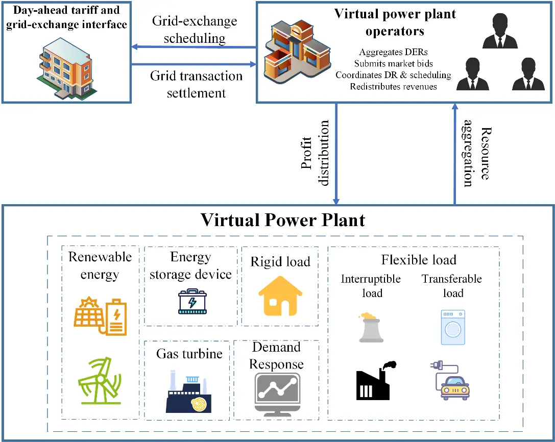
Figure 1. Schematic of the renewable-based VPP operating structure for internal source-storage-load coordination.
The revenue-related arrows in Figure 1 illustrate generic functions of a VPP operator and are included only as contextual information. Revenue allocation is neither an optimization decision nor a research objective in the present scheduling model. The main GT and ESS parameter settings are summarized in Table 2.
Table 2. Parameter settings of gas turbine units and energy storage systems.
|
Gas Turbine Units |
Energy Storage System |
||
|---|---|---|---|
|
Parameter |
Value |
Parameter |
Value |
|
Rated power (MW) |
30 |
Rated capacity (MWh) |
200 |
|
Number of units |
4 |
Rated power (MW) |
50 |
|
Cost coefficient a |
0.008 |
SOC range |
0.1–0.9 |
|
Cost coefficient b |
35 |
Initial SOC |
0.5 |
|
Cost coefficient c |
20 |
Efficiency |
0.98 |
The remaining cost, reserve, forecast-deviation, and demand-response parameters are kept identical across all comparative cases. The time-of-use purchase and selling prices are summarized in Table 3.
Table 3. Electricity purchase and selling prices in different time periods.
|
Period |
Time Range (h) |
Purchase Price ($/MWh) |
Selling Price ($/MWh) |
|---|---|---|---|
|
Valley period I |
1–4 |
24.75 |
17.33 |
|
High-peak period |
5–8 |
207.26 |
145.08 |
|
Valley period II |
9–12 |
27.16 |
19.01 |
|
Flat period I |
13–17 |
38.63 |
27.04 |
|
Peak period |
18–21 |
85.61 |
59.93 |
|
Flat period II |
22–24 |
40.59 |
28.41 |
Figure 2 shows the load-error band to characterize the uncertainty level of the input operating day. In the present deterministic implementation, the explicit reserve requirements are constructed from the wind and PV forecast-deviation margins.
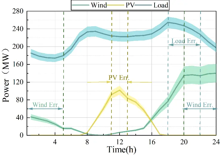
Figure 2. Forecast-deviation bands for wind power, PV generation, and load trajectories under the studied operating day.
3.2. Comparative Model Design
Three models are compared. The baseline model maximizes short-term net operating profit under the same physical constraints. The scalarized multi-term reference model includes economic and operating-coordination terms but does not include the FLI term. The proposed FLI model adds the normalized RE, ES, and FL indicators with the baseline weight ratio $$K_{\mathrm{RE}}: K_{\mathrm{ES}}: K_{\mathrm{FL}} = 1:1:1$$ and $$S_{\mathrm{FLI}} = 2.5$$. Renewable utilization is imposed as a common constraint in all three models.
To ensure consistency, the no-FLI ablation case was checked against the scalarized multi-term reference model. The objective difference was zero within solver tolerance, the maximum dispatch-variable difference was zero, and the main-case power-balance residual was 5.68 × 10⁻¹⁴. This confirms that removing all FLI channels numerically reproduces the non-FLI scalarized formulation. The operational metrics used in the comparative analysis are defined in Section 2.4.
3.3. Main-Case Dispatch Comparison
The main-case results show that the proposed FLI schedule changes resource use through a flexibility-preservation trade-off rather than through unconditional profit maximization. Net operating profit was 69,590.98 USD for the baseline, 60,377.26 USD for the scalarized multi-term reference model, and 66,856.81 USD for the proposed FLI model. Thus, the proposed FLI model accepted a 3.93% profit concession relative to the baseline but improved profit by 10.73% relative to the scalarized multi-term reference model.
Figure 3 shows that the proposed FLI model modifies the aggregate GT output trajectory and the internal substitution among GT generation, storage operation, grid exchange, and demand-side flexibility while keeping feasibility and renewable accommodation unchanged. The result should be interpreted as a change in internal resource substitution, not as evidence of universal GT-output reduction.
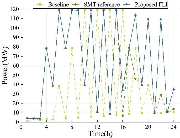
Figure 3. Comparison of aggregate gas-turbine output trajectories under the three scheduling models.
Figure 4 illustrates the system-level redistribution of shiftable load under the three schedules. Because the FL indicator in Equation (26) is defined in terms of interruptible-load activation, this SL figure is interpreted as an indirect load-side scheduling response rather than as direct evidence of the FL indicator itself. The No-FL ablation and multi-scenario activation diagnostics provide direct FL-channel evidence.
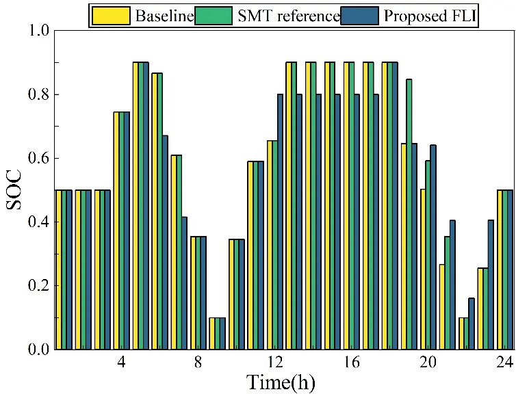
Figure 5 and Table 4 show the clearest main-case effect of the ES channel. SOC boundary contacts decreased from 9 to 3, corresponding to a 66.7% reduction, while equivalent full cycles decreased from 1.7253 to 1.6647, or approximately 3.51%. This indicates a shift from boundary-following arbitrage toward partial storage-state preservation.
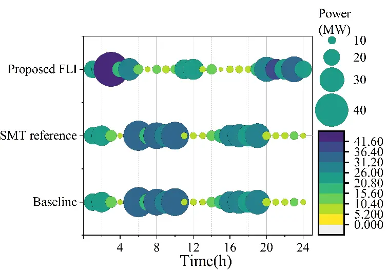
Figure 4. Comparison of shiftable-load power under the three scheduling models. Bubble size and color intensity represent the magnitude of shiftable-load dispatch. SMT reference denotes the scalarized multi-term reference model, and Proposed denotes the proposed FLI model.
Table 4. Main-case economic and operational performance under the three dispatch models.
|
Metric |
Baseline |
SMT Reference |
Proposed FLI |
|---|---|---|---|
|
Net operating profit (USD) |
69,590.98 |
60,377.26 |
66,856.81 |
|
Profit vs. Baseline (%) |
0.00 |
−13.24 |
−3.93 |
|
Profit vs. SMT reference (%) |
15.26 |
0.00 |
10.73 |
|
SOC boundary contacts |
9 |
9 |
3 |
|
SOC mean |
0.5973 |
0.6130 |
0.5865 |
|
ESS throughput (MWh) |
690.13 |
690.13 |
665.90 |
|
Equivalent full cycles |
1.7253 |
1.7253 |
1.6647 |
|
GT ramping total (MW) |
399.09 |
430.40 |
403.71 |
|
SL shifted energy (MWh) |
214.67 |
214.67 |
210.75 |
|
Renewable utilization |
1.0000 |
1.0000 |
1.0000 |
|
Renewable curtailment (MWh) |
<1 × 10⁻¹² |
<1 × 10⁻¹² |
<1 × 10⁻¹² |
SMT reference denotes the scalarized multi-term reference model. Values reported as <1 × 10⁻¹² are below this threshold in the adopted reporting unit.
Raw FLI and reference-scale values are expressed in USD. Normalized and weighted FLI components are dimensionless. The weighted component represents the inner channel weight multiplied by the normalized channel value and does not independently equal the final monetary contribution in the scalar objective.
As reported in Table 5, the RE component is nearly zero in the main case because available wind and PV power are almost fully accommodated. The ES and FL components, therefore, dominate the normalized FLI value in this operating condition.
Table 5. Raw, normalized, and weighted FLI components in the proposed FLI main case.
|
Component |
Raw FLI (USD) |
Reference Scale (USD) |
Normalized FLI (-) |
Weighted FLI (-) |
|---|---|---|---|---|
|
RE |
1.62 × 10⁻¹¹ |
59,145.64 |
2.74 × 10⁻¹⁶ |
9.14 × 10⁻¹⁷ |
|
ES |
4883.44 |
87,344.09 |
0.05591 |
0.01864 |
|
FL |
1252.38 |
18,514.80 |
0.06764 |
0.02255 |
3.4. Weight Sensitivity Analysis
To test whether the result depends on the equal 1:1:1 coefficient setting, seven alternative RE:ES:FL weight ratios were examined: 1:1:1, 2:1:1, 1:2:1, 1:1:2, 0.5:1:1, 1:0.5:1, and 1:1:0.5. Each ratio was internally normalized so that the three coefficients summed to one, while the input data, reference scales, s_FLI, and solver settings were kept fixed.
Figure 6 shows that the storage response is governed primarily by the ES-channel weight. Across the seven cases, net operating profit ranged from 66,609.02 USD to 68,403.97 USD, SOC boundary contacts ranged from 3 to 9, and EFC ranged from 1.6253 to 1.7253. The high-ES case (1:2:1) produced the lowest EFC, while low-ES or high non-ES cases returned to 9 boundary contacts and an EFC of 1.7253. Thus, the effect is not an artifact of the single 1:1:1 point, but it does show a clear threshold dependence on the ES-channel weight. Renewable curtailment remained approximately 2.27 × 10⁻¹³ MWh in all weight cases, confirming that the RE channel had no curtailment margin to act on in this main operating condition.
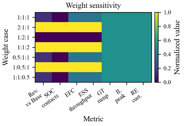
Figure 6. Weight-sensitivity results of the proposed FLI model. Each column is normalized across the seven weight cases.
3.5. Channel Ablation Analysis
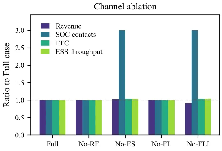
Channel ablation was used to test whether the three indicators act as distinguishable coordination signals. The Full case includes all three channels; No-RE, No-ES, and No-FL remove one channel at a time, and No-FLI removes all FLI channels. The ablation is non-redistributed: the original one-third coefficients are normalized before enabling flags are applied, and a disabled channel is set to zero without reassigning its coefficient to the remaining channels.
As shown in Figure 7, removing the ES channel increased SOC boundary contacts from 3 to 9 and increased EFC from 1.6647 to 1.7253 relative to the Full case, confirming that the storage-side indicator provides a distinct inter-temporal coordination signal. No-FLI reproduced the scalarized multi-term reference model, which verifies implementation consistency. The RE and FL channels produced weaker differences in the main case because renewable curtailment was nearly zero, and the main-case IL activation pattern was not strongly differentiated.
3.6. Multi-Scenario Validation
To reduce reliance on a single operating day, the study evaluated eight representative operating and stress-test scenarios. These scenarios were generated by scaling the 20 November 2024 PJM-based trajectories and should be interpreted as operating-state and stress-test extensions of the available dataset, not as independent multi-season historical operating days. For the multi-scenario ablation, the reference scales were recalculated once from each scenario’s input data and then kept fixed across the Full, No-RE, No-ES, No-FL, and No-FLI variants within that scenario; cross-scenario comparisons therefore emphasize within-scenario channel effects rather than absolute FLI-scale magnitudes. The scenario settings used for multi-scenario validation are summarized in Table 6.
Table 6. Representative operating and stress-test scenarios used for multi-scenario validation.
|
Scenario |
Group |
Load |
Wind |
PV |
Price |
IL Capacity Ratio |
Uncert. |
Purpose |
|---|---|---|---|---|---|---|---|---|
|
Base operating |
Representative |
1.00 |
1.00 |
1.00 |
1.00 |
0.40 |
1.00 |
Main PJM-scaled operating day |
|
Renewable-rich |
Representative |
0.94 |
1.18 |
1.28 |
1.00 |
0.45 |
0.85 |
Higher renewable availability and lower net load |
|
Evening peak |
Representative |
1.12 |
0.92 |
0.82 |
1.18 |
0.45 |
1.15 |
Evening load ramp and high peak price |
|
Flexible-load-rich |
Representative |
1.06 |
1.00 |
0.95 |
1.28 |
0.55 |
1.00 |
Larger flexible-load pool |
|
Renewable-surplus stress |
Stress test |
0.84 |
1.45 |
1.55 |
0.94 |
0.45 |
0.80 |
High renewable input and low midday load |
|
Storage-ramp stress |
Stress test |
1.14 |
0.88 |
0.82 |
1.20 |
0.45 |
1.25 |
Steep net-load ramp and forecast uncertainty |
|
Flexible-load peak stress |
Stress test |
1.16 |
0.96 |
0.90 |
1.75 |
0.65 |
1.05 |
High peak price and flexible-load capacity |
|
Combined stress |
Stress test |
1.08 |
1.18 |
1.18 |
1.38 |
0.58 |
1.12 |
Combined renewable, ramp, and load-side stress |
The listed load, wind, PV, price, and uncertainty entries are dimensionless base multipliers. The uncertainty multiplier scales the wind/PV forecast-deviation bands used in scenario construction. The IL capacity ratio is the share of baseline interruptible load that can be activated and is therefore not a multiplier. Three smooth time-window modifiers are then applied where relevant: morning is centered at hour 8 with standard deviation 2.6 h, midday is centered at hour 13 with standard deviation 3.0 h, and evening is centered at hour 19 with standard deviation 2.8 h.
The additional modifiers are as follows. Renewable-rich operation applies load −0.08 midday and +0.03 evening, wind +0.10 morning, PV +0.18 midday, and price +0.05 evening. Evening-peak operation applies load +0.28 evening, PV −0.12 evening, and price +0.35 evening. Flexible-load-rich operation applies load +0.18 evening and price +0.55 evening. Renewable-surplus stress applies load −0.16 midday, wind +0.18 morning, PV +0.28 midday, and price −0.08 midday. Storage-ramp stress applies load −0.06 midday and +0.30 evening, wind +0.08 morning, PV −0.18 evening, and price +0.50 evening. Flexible-load peak stress applies load +0.34 evening, PV −0.10 evening, and price +0.95 evening. Combined stress applies load −0.08 midday and +0.28 evening, wind +0.12 morning, PV +0.14 midday and −0.06 evening, and price +0.70 evening and −0.10 midday.
The scenario feature map uses four normalized descriptors: renewable-to-load is total available renewable energy divided by total load energy; net-load ramp is the sum of absolute hourly net-load changes; IL capacity is the total available interruptible-load capacity after applying the scenario ratio; and peak-to-mean price is the ratio between the maximum hourly tariff and the daily mean tariff. In Figure 8, Peak, RE-stress, ES-stress, and FL-stress denote evening-peak, renewable-surplus-stress, storage-ramp-stress, and flexible-load-peak-stress scenarios, respectively.
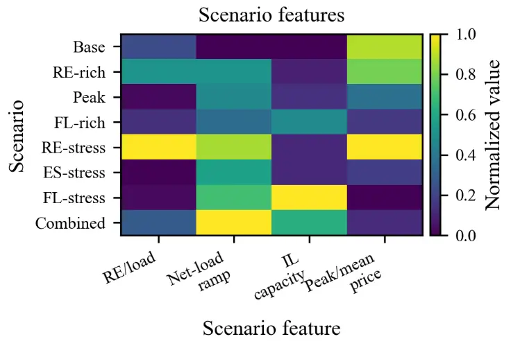
Figure 9 uses a normalized signed log-scaled effect to display positive and negative ablation effects on a common scale. For each metric, the Full-versus-No-channel difference is first divided by the maximum absolute difference of that metric across the eight scenarios, and the signed log transform is then applied. When the maximum absolute difference of a metric is below its numerical activity threshold across all scenarios, the normalized effect is assigned a value of zero in the visualization. Thus, the displayed bars compare relative within-metric effects rather than raw differences in MWh, MW, or dimensionless EFC. A channel is regarded as active when disabling it changes its corresponding physical metric beyond the specified numerical activity threshold: renewable curtailment > 1 × 10⁻⁶ MWh or utilization > 1 × 10⁻⁸ for RE; EFC > 1 × 10⁻⁶, ESS throughput > 1 × 10⁻⁵ MWh, or an integer SOC-boundary-contact change of at least one period for ES; and IL total activation or peak activation > 1 × 10⁻⁵ MW or MWh for FL. Changes in SL shifted energy are reported only as indirect system-level load-side responses because SL does not directly enter the FL indicator in Equation (26). Figure 9 displays one representative physical metric for each channel, whereas the reported channel-activity counts are determined using the complete channel-specific metric set described above.
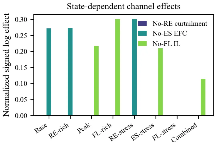
Figure 9. State-dependent channel effects across the representative operating and stress-test scenarios.
All 40 scenario-ablation optimization problems were solved successfully. The maximum power-balance residual was 1.14 × 10⁻¹³, and terminal SOC residuals were zero within numerical tolerance. Across the eight scenarios, the ES channel was active in 7 cases, the FL channel was active in 4 cases, and the RE channel was active in 0 cases. The FL channel was visible in the evening-peak, flexible-load-rich, storage-ramp-stress, and combined-stress scenarios. The RE channel remained inactive because renewable curtailment was essentially zero under the current market-interface assumption.
3.7. Discussion
The results support a bounded interpretation of the FLI framework. The main effect is not a universal increase in short-term profit, but a dispatch trade-off that preserves storage flexibility and changes resource allocation under selected operating states.
First, the ES channel is the most stable and directly observable channel. In the main case, it reduced SOC boundary contacts from 9 to 3 and reduced equivalent full cycles from 1.7253 to 1.6647. Across the representative and stress-test scenarios, removing the ES channel affected SOC-related metrics in 7 of 8 cases, indicating that the storage-side indicator is transmitted through real inter-temporal decisions rather than through a purely accounting term.
Second, the FL channel is state dependent. It is weak in the main operating day but becomes active in the evening-peak, flexible-load-rich, storage-ramp-stress, and combined-stress scenarios. This suggests that the interruptible-load indicator should be interpreted as a conditional coordination signal whose effect depends on whether load-side flexibility is actually marginal in the dispatch problem.
Third, the RE channel is structurally coupled to the optimization model because scheduled wind and PV outputs enter the power-balance equation, renewable utilization, curtailment, and the RE-FLI term consistently. Nevertheless, its marginal effect is limited in the tested cases because wind and PV are almost fully accommodated. The RE activation-space audit also showed no explicit grid-export upper bound, which helps explain why renewable curtailment remains approximately zero. Therefore, the RE channel is treated as a correctly implemented but inactive channel under the current operating and market-interface assumptions.
From an economic perspective, the proposed model should be understood as a flexibility-preservation trade-off. It accepted an approximately 3.93% short-term profit concession relative to the profit-oriented baseline in exchange for a 66.7% reduction in SOC boundary contacts and a 3.51% reduction in equivalent full cycles. This is a more defensible interpretation than claiming that the FLI model is economically superior in all respects.
The main limitation is that the multi-scenario tests are representative operating and stress-test scenarios derived from the available dataset rather than independent multi-season historical operating days. Additional validation with multi-season PJM data, explicit export-capacity limits, stochastic forecast scenarios, and multi-market settlement rules would be needed before generalizing the relative contribution of the RE, ES, and FL channels.
4. Conclusions
This paper presents a normalized flexibility-loss-indicator scheduling framework for a renewable VPP with energy storage and demand flexibility. The framework uses a bounded engineering interpretation: RE, ES, and FL indicators quantify selected flexibility losses and enter the dispatch objective through fixed reference-scale normalization and explicit channel weights.
The main case shows that the proposed model provides a trade-off rather than a universal economic improvement. Compared with the baseline, the proposed FLI model reduced net operating profit by 3.93% and reduced SOC boundary contacts from 9 to 3 and equivalent full cycles from 1.7253 to 1.6647. Compared with the scalarized multi-term reference model, it increased net operating profit by 10.73% while retaining the SOC-preservation effect.
Weight-sensitivity and ablation analyses indicate that the storage benefit is not unique to the 1:1:1 setting, although its magnitude shows a clear dependence on the ES-channel weight, and that the ES channel has a distinct operational effect. Multi-scenario validation further shows that the FL channel is activated under peak-load and flexibility-stressed conditions, whereas the RE channel remains weak because renewable curtailment is nearly zero under the present assumptions. These findings support the conclusion that FLI contributions are state dependent.
Future work should extend the framework to historical multi-season typical days, explicit export-capacity and market-interface constraints, stochastic or robust scenario sets, and multi-VPP or multi-market coordination. Such extensions would help determine when the renewable-side channel becomes marginal and how FLI weights should be calibrated for operational deployment.
Author Contributions
L.J.: Conceptualization, Methodology, Software, Formal analysis, Writing-original draft. Y.G.: Supervision, Project administration, Funding acquisition, Writing-review and editing. R.B.: Validation, Data curation, Investigation. Q.W.: Resources, Data curation, Validation. W.X.: Investigation, Resources, Validation. Y.O.: Methodology, Software, Visualization. Y.J.: Formal analysis, Investigation, Visualization. L.Q.: Writing-review and editing, Validation.
Ethics Statement
Not applicable.
Informed Consent Statement
Not applicable.
Data Availability Statement
The data that support the findings of this study are available from the corresponding author upon reasonable request.
Funding
This work was supported by the Science and Technology Project of State Grid Heilongjiang Electric Power Co., Ltd. (522400250007).
Declaration of Competing Interest
The authors declare that they have no known competing financial interests or personal relationships that could have appeared to influence the work reported in this paper.
References
- Zhu J, Gao M, Xiao P, Dong H, Zhu H, Lin K. Review of offshore wind power grid integration and operation in new energy systems. Smart Energy Syst. Res. 2026, 2, 10002. DOI:10.70322/sesr.2026.10002 [Google Scholar]
- Zhang S, Lu Y, Huang Q, Liu M. Hybrid encoder-decoder model for ultra-short-term prediction of wind farm power. Smart Energy Syst. Res. 2025, 1, 10004. DOI:10.70322/sesr.2025.10004 [Google Scholar]
- Nassreddine G, Hellany A, Al-Khatib O, Rammal A, Nassereddine M. Feature selection technique using multiple linear regression for accurate electricity demand forecasting. Smart Energy Syst. Res. 2025, 1, 10003. DOI:10.70322/sesr.2025.10003 [Google Scholar]
- Shafiekhani M, Ahmadi A, Homaee O, Shafie-khah M, Catalao JPS. Optimal bidding strategy of a renewable-based virtual power plant including wind and solar units and dispatchable loads. Energy 2022, 239, 122379. DOI:10.1016/j.energy.2021.122379 [Google Scholar]
- Shui J, Peng D, Zeng H, Song Y, Yu Z, Yuan X, et al. Optimal scheduling of multiple entities in virtual power plant based on the master-slave game. Appl. Energy 2024, 376, 124286. DOI:10.1016/j.apenergy.2024.124286 [Google Scholar]
- Fang F, Yu S, Xin X. Data-driven-based stochastic robust optimization for a virtual power plant with multiple uncertainties. IEEE Trans. Power Syst. 2022, 37, 456–466. DOI:10.1109/TPWRS.2021.3091879 [Google Scholar]
- Naughton J, Wang H, Cantoni M, Mancarella P. Co-optimizing virtual power plant services under uncertainty: A robust scheduling and receding horizon dispatch approach. IEEE Trans. Power Syst. 2021, 36, 3960–3972. DOI:10.1109/TPWRS.2021.3062582 [Google Scholar]
- Zhang Y, Liu F, Wang Z, Su Y, Wang W, Feng S. Robust scheduling of virtual power plant under exogenous and endogenous uncertainties. IEEE Trans. Power Syst. 2022, 37, 1311–1325. DOI:10.1109/TPWRS.2021.3105418 [Google Scholar]
- Li Z, Hilber P, Li Z, Laneryd T, Ivanell S. Temporally coordinated operation of green multi-energy airport microgrids with climatic correlations and flexible loads via decomposed stochastic programming. IEEE Trans. Sustain. Energy 2026, 17, 1909–1922. DOI:10.1109/TSTE.2025.3639360 [Google Scholar]
- Zeng X, Zheng X, Chen H, Yin X, Li Z, Chen Y. Deriving the robust operating region for multistage dispatch of power systems: A decision-dependent uncertainties based modeling approach. IEEE Trans. Sustain. Energy 2026, 17, 3019–3032. DOI:10.1109/TSTE.2026.3663924 [Google Scholar]
- Xiao D, Lin Z, Chen H, Hua W, Yan J. Windfall profit-aware stochastic scheduling strategy for industrial virtual power plant with integrated risk-seeking/averse preferences. Appl. Energy 2024, 357, 122460. DOI:10.1016/j.apenergy.2023.122460 [Google Scholar]
- Ma Y, Li Z, Liu R, Liu B, Yu SS, Liao X, et al. Data-driven interval robust optimization method of VPP bidding strategy in spot market under multiple uncertainties. Appl. Energy 2025, 384, 125366. DOI:10.1016/j.apenergy.2025.125366 [Google Scholar]
- She B, Xiao JW, Wang YW, He SY. Decision-driven uncertainty management in multi-energy virtual power plant: A robust multi-market scheduling framework. J. Clean. Prod. 2025, 527, 146688. DOI:10.1016/j.jclepro.2025.146688 [Google Scholar]
- Zhou Y, Essayeh C, Morstyn T. A novel surrogate polytope method for day-ahead virtual power plant scheduling with joint probabilistic constraints. Electr. Power Syst. Res. 2024, 234, 110623. DOI:10.1016/j.epsr.2024.110623 [Google Scholar]
- Wei X, Xu Y, Sun H, Bai X, Chang X, Xue Y. Day-ahead optimal dispatch of a virtual power plant in the joint energy-reserve-carbon market. Appl. Energy 2024, 356, 122459. DOI:10.1016/j.apenergy.2023.122459 [Google Scholar]
- Chen Y, Niu Y, Qu C, Du M, Liu P. A pricing strategy based on bi-level stochastic optimization for virtual power plant trading in multi-market: Energy, ancillary services and carbon trading market. Electr. Power Syst. Res. 2024, 231, 110371. DOI:10.1016/j.epsr.2024.110371 [Google Scholar]
- Pandey AK, Jadoun VK, Jayalakshmi NS, Malik H, Garcia Marquez FP. Multi-objective price based flexible reserve scheduling of virtual power plant. Renew. Sustain. Energy Rev. 2024, 192, 114218. DOI:10.1016/j.rser.2023.114218 [Google Scholar]
- Nguyen Hong N, Nguyen Duc H. Virtual power plant’s optimal scheduling strategy in day-ahead and balancing markets considering reserve provision model of energy storage system. Appl. Sci. 2024, 14, 2175. DOI:10.3390/app14052175 [Google Scholar]
- Feng C, Huang Z, Lin J, Wang L, Zhang Y, Wen F. Aggregation model and market mechanism for virtual power plant participation in inertia and primary frequency response. IEEE Trans. Power Syst. 2026, 41, 2101–2117. DOI:10.1109/TPWRS.2025.3637538 [Google Scholar]
- Qin W, Li X, Jing X, Zhu Z, Lu R, Han X. Multi-temporal optimization of virtual power plant in energy-frequency regulation market under uncertainties. J. Mod. Power Syst. Clean Energy 2025, 13, 675–687. DOI:10.35833/MPCE.2024.000118 [Google Scholar]
- Lu X, Qiu J, Zhang C, Lei G, Zhu J. Assembly and competition for virtual power plants with multiple ESPs through a recruitment-participation approach. IEEE Trans. Power Syst. 2024, 39, 4382–4396. DOI:10.1109/TPWRS.2023.3296738 [Google Scholar]
- Shang Y, Li X, Xu T, Cui L. Uncertainty-output virtual power plant participates in multi-electricity market considering the improved Shapley value distribution method. Int. J. Electr. Power Energy Syst. 2025, 165, 110462. DOI:10.1016/j.ijepes.2025.110462 [Google Scholar]
- Schiro DA, Zheng T, Zhao F, Litvinov E. Convex hull pricing in electricity markets: Formulation, analysis, and implementation challenges. IEEE Trans. Power Syst. 2016, 31, 4068–4075. DOI:10.1109/TPWRS.2015.2486380 [Google Scholar]
- Harsh P, Sun H, Das D, Rameshrao AG, Jiang J. Stochastic incentive-based demand response program for virtual power plant with distributed energy resources. IEEE Trans. Ind. Appl. 2025, 61, 4862–4875. DOI:10.1109/TIA.2025.3535847 [Google Scholar]
- Zhou K, Peng N, Yin H, Hu R. Urban virtual power plant operation optimization with incentive-based demand response. Energy 2023, 282, 128700. DOI:10.1016/j.energy.2023.128700 [Google Scholar]
- Ryu J, Kim J. Virtual power plant operation strategy under uncertainty with demand response resources in electricity markets. IEEE Access 2022, 10, 62763–62771. DOI:10.1109/ACCESS.2022.3181163 [Google Scholar]
- Wu JK, Liu ZW, Li C, Zhao Y, Chi M. Coordinated operation strategy of virtual power plant based on two-layer game approach. IEEE Trans. Smart Grid 2025, 16, 554–567. DOI:10.1109/TSG.2024.3440315 [Google Scholar]
- Yi Z, Xu Y, Wang H, Sang L. Coordinated operation strategy for a virtual power plant with multiple DER aggregators. IEEE Trans. Sustain. Energy 2021, 12, 2445–2458. DOI:10.1109/TSTE.2021.3100088 [Google Scholar]
- Ren J, Zeng Y, Qin C, Li B, Wang Z, Yuan Q, et al. Characterization and application of flexible operation region of virtual power plant. Appl. Energy 2024, 371, 123733. DOI:10.1016/j.apenergy.2024.123733 [Google Scholar]
- Finke J, Bertsch V. Implementing a highly adaptable method for the multi-objective optimisation of energy systems. Appl. Energy 2023, 332, 120521. DOI:10.1016/j.apenergy.2022.120521 [Google Scholar]
- Li Q, Zhou Y, Wei F, Li S, Wang Z, Li J, et al. Multi-time scale scheduling for virtual power plants: Integrating the flexibility of power generation and multi-user loads while considering the capacity degradation of energy storage systems. Appl. Energy 2024, 362, 122980. DOI:10.1016/j.apenergy.2024.122980 [Google Scholar]
- Yan X, Gao C, Francois B. Multi-objective optimization of a virtual power plant with mobile energy storage for a multi-stakeholders energy community. Appl. Energy 2025, 386, 125553. DOI:10.1016/j.apenergy.2025.125553 [Google Scholar]
- Ghanuni A, Sharifi R, Farahani HF. A risk-based multi-objective energy scheduling and bidding strategy for a technical virtual power plant. Electr. Power Syst. Res. 2023, 220, 109344. DOI:10.1016/j.epsr.2023.109344 [Google Scholar]