
Multi-Objective Optimization Design of An Integrated Energy System with Ice Storage Based on Deep Reinforcement Learning

Multi-Objective Optimization Design of An Integrated Energy System with Ice Storage Based on Deep Reinforcement Learning
Received: 22 May 2026 Revised: 09 June 2026 Accepted: 29 June 2026 Published: 03 July 2026

© 2026 The authors. This is an open access article under the Creative Commons Attribution 4.0 International License (https://creativecommons.org/licenses/by/4.0/).
1. Introduction
Buildings account for over one-third of global energy consumption [1], significantly contributing to carbon emissions. To achieve carbon neutrality, transitioning building energy systems into distributed energy systems (DESs) has become a critical pathway. By integrating renewable energy (RE) generation and energy storage systems (ESSs), DESs can enhance energy efficiency and improve energy supply independence [2]. However, the intermittency of RE generation, dynamic load fluctuations [3], and thermoelectric coupling effects [4] pose substantial challenges in the optimal design of DESs [5].
The power generation characteristics of RE sources such as photovoltaic (PV) and wind power are highly dependent on weather conditions [6], exhibiting inherent intermittency and volatility. PV output follows diurnal periodic patterns driven by solar irradiance but is subject to random variations caused by cloud cover. Wind power displays more pronounced stochastic variability due to spatiotemporal variations in wind speed. To predict the renewable energy generation, current research has primarily focused on two approaches: mathematical modeling and data-driven forecasting. Zhu et al. [7] applied a mathematical model that linked PV output to solar irradiance and temperature, and correlated wind power with wind speed. By integrating equipment parameters and meteorological data, the model captures the dynamic behavior of RE generation. Hua et al. [8] employed stochastic modeling, characterizing wind speed variations using a Weibull distribution and solar irradiance fluctuations via a Beta distribution. Their probabilistic framework quantifies RE volatility through probability density functions (PDFs), assessing its impact on power system stability. With the widespread adoption of smart sensors, machine learning models have proven effective for PV generation forecasting [9] and short-term load profile prediction [10]. While early studies relied on conventional models such as autoregressive integrated moving average (ARIMA) and support vector machines (SVMs), recent advances in deep learning have demonstrated the superior temporal modeling capabilities of Long Short-Term Memory (LSTM) networks for RE prediction [11]. Wang et al. [12] developed an LSTM-based approach for PV forecasting that integrates ensemble empirical mode decomposition (EEMD) for data preprocessing and Bayesian optimization for hyperparameter tuning. Experimental results demonstrate the model’s superior performance, achieving a root mean square error (RMSE) of 4.157 for 7-day-ahead forecasting, with a 15% improvement in accuracy over conventional methods. Chen et al. [13] developed an LSTM-based approach for wind power forecasting, which combines numerical weather prediction data with turbine monitoring measurements. The proposed LSTM model framework effectively captures temporal characteristics across multiple turbines, outperforming tradition prediction models in distributed wind farm applications.
The dynamic RE generation and fluctuating building loads often lead to supply-demand imbalance [14]. A notable example is the midday solar overgeneration contrasted with evening supply shortages, when PV output declines sharply, and wind generation may simultaneously drop to low levels [15]. To address the temporal mismatch between RE generation and energy demand, ESSs are essential for maintaining grid stability. Battery storage serves as the primary solution for storing surplus renewable electricity, which can then be discharged during periods of insufficient generation. For cooling-dominated buildings, ice thermal energy storage (ITES) systems offer distinct advantages by enabling the temporal shifting of cooling loads to periods of RE surplus, thereby enhancing renewable penetration [16]. This hybrid system, constructed on the principle of “renewable energy coupled with energy storage”, not only achieves significant peak shaving and valley filling effects but also enhances the grid’s absorption capacity for renewable energy through multi-energy complementarity [17]. Studies have revealed the significant benefits of such integrated systems. Saffari et al. [18] demonstrated that combining ITES with RE could result in a 30% annual cost savings. In a case study in Qatar [19,20], the combination of RE and ESS substantially reduced carbon emissions and gas dependency of the power system. Odufuwa et al. [21] developed a PV-integrated ice-thermal storage system. Its effectiveness was proved through optimization, resulting in approximately 33% annual energy cost savings. Christoph Luerssen et al. [22] assessed the net present value (NPV) of various PV-powered cooling system configurations. The results showed that the combination of RE with batteries and thermal storage significantly reduced fuel costs while achieving competitive economics. Similarly, Arévalo et al. [23] conducted a techno-economic evaluation of hybrid renewable systems combining photovoltaic, wind, hydrokinetic, and diesel sources, demonstrating that energy management strategies under site-specific conditions significantly affect system cost, emissions, and renewable penetration.
While hybrid energy systems integrate multiple devices to ensure energy supply, the design optimization of these systems is paramount for enhancing their efficiency, reliability, and economic viability. Conventional approaches typically determine equipment capacity based on peak load demands, resulting in system overcapacity and resource wastage [24]. To bridge the gap, advanced meta-heuristic algorithms have been widely adopted, including Particle Swarm Optimization (PSO) [25], Genetic Algorithms (GA) [26], Ant Colony Optimization (ACO) [27], and Evolutionary Mating Algorithm (EMA) [28]. Despite their effectiveness under specific conditions, metaheuristic algorithms exhibit notable limitations. One major drawback lies in their sensitivity to parameter settings. For instance, the performance of PSO largely depends on the selection of inertia weights and learning factors, while the effectiveness of GA is strongly influenced by crossover and mutation rates. Improper parameter configurations can lead to slow convergence or even failure to converge, rendering these algorithms ineffective in handling dynamic models under complex environments [29].
Deep Reinforcement Learning (DRL) has emerged as a powerful approach for addressing the aforementioned challenges, as it is capable of executing autonomous decisions in complex environments [30]. DRL agents learn optimal control policies through continuous interaction with the environment [31]. This capability makes them particularly suitable for handling uncertainties in hybrid energy systems that integrate multiple sources for energy supply.
Among various DRL algorithms, Proximal Policy Optimization (PPO) has demonstrated superior stability and sample efficiency. It has been successfully tested in energy management [32]. In the context of low-carbon park energy dispatch, Ning et al. [33] developed a PPO-Mix Clip algorithm, with experimental results demonstrating a 3.52% reduction in daily operational costs. For the coordinated optimization of electric vehicles and smart homes, the HEN-PPO approach achieved energy savings ranging from 24% to 29% [34]. Le et al. [35] proposed the DAL-PPO method, which innovatively integrates energy efficiency optimization, indoor comfort maintenance, and system robustness enhancement into a unified reward function, with experimental findings indicating substantial performance improvements within the single-objective optimization framework.
Regarding multi-objective optimization, Ge et al. [36] proposed a multi-objective DRL (MODRL) method for scheduling of wind-solar-hydro-battery complementary system. Compared to NSGA-II, the solutions provided by the MODRL approach were closer to the true Pareto front (PF). However, significant research gaps persist in MODRL applications for building energy system design. Although conventional optimization methods can achieve multi-objective optimization in building energy systems, these approaches often rely on precise mathematical models and struggle to adapt to highly dynamic building energy environments. Deep reinforcement learning (DRL), with its capability to handle high-dimensional state spaces and learn complex nonlinear policies, is particularly suitable for addressing decision-making problems in multi-objective optimization of building energy systems. The development of building-oriented multi-objective DRL frameworks enables autonomous perception of environmental states and learning of optimal control strategies, effectively coordinating the trade-offs among economic viability, environmental sustainability, and energy efficiency. Such frameworks can effectively resolve inherent conflicting mechanisms among objectives and explore Pareto-optimal solution sets, thereby enabling holistic system-wide optimal design.
This study proposes an innovative design strategy for integrated energy systems with high renewable energy penetration by introducing an adaptive reward mechanism to dynamically balance multi-objective optimization. The main contributions are as follows: (1) A novel integrated energy system (IES) architecture is developed, incorporating PV and wind power generation units, a battery, and ITES devices with nonlinear ice-melting characteristics. A time series prediction model based on a LSTM neural network is established for renewable power generation forecasting. (2) The system incorporates an advanced ice thermal energy storage model that accounts for nonlinear ice-melting characteristics, accurately capturing the phase-change heat transfer process of ITES devices. (3) An improved Multi-Objective Proximal Policy Optimization (MOPPO) algorithm is proposed, employing life cycle cost (LCC), carbon dioxide emission reduction rate (CDERR), and renewable energy utilization (RU) as objective functions to optimize system capacity allocation. This algorithm searches for Pareto optimal solutions through policy gradient methods.
2. Methodology
This study proposes a hybrid methodology that integrates mathematical modeling and data-driven prediction to construct IES models, using an improved multi-objective reinforcement learning approach to achieve multi-objective collaborative optimization. The research is structured around the following key areas: (1) Development of an IES: integrating LSTM neural network-based prediction models with physics-based mathematical models for system construction. (2) Optimal design of the IES: from a multi-objective perspective, prioritizing three primary objectives—economic efficiency, environmental impact, and energy sustainability, while accounting for the system’s operational constraints. (3) Solution methodology for the IES: The optimal design problem is formulated as a Markov Decision Process (MDP) through the definition of the state space, action space, and reward function, with optimal design solutions obtained through an improved reinforcement learning-based policy iteration optimization algorithm.
2.1. System Description
The overall system architecture and energy flow are illustrated in Figure 1. It presents an IES that incorporates PV, WT generation, ITES, battery storage, two types of dual-duty chillers with different rated cooling capacities, water pumps, and the power grid. The dual-duty chillers operate in a “daytime cooling and nighttime ice-making” mode, providing cooling services for buildings during the day and producing ice for thermal storage during periods of low nighttime electricity demand, thereby shifting energy consumption.
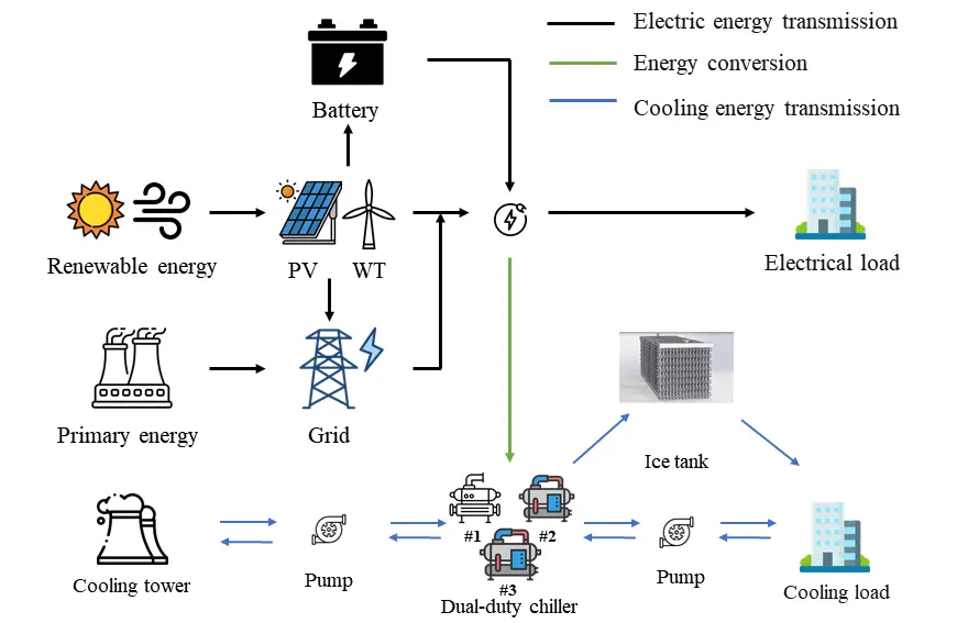
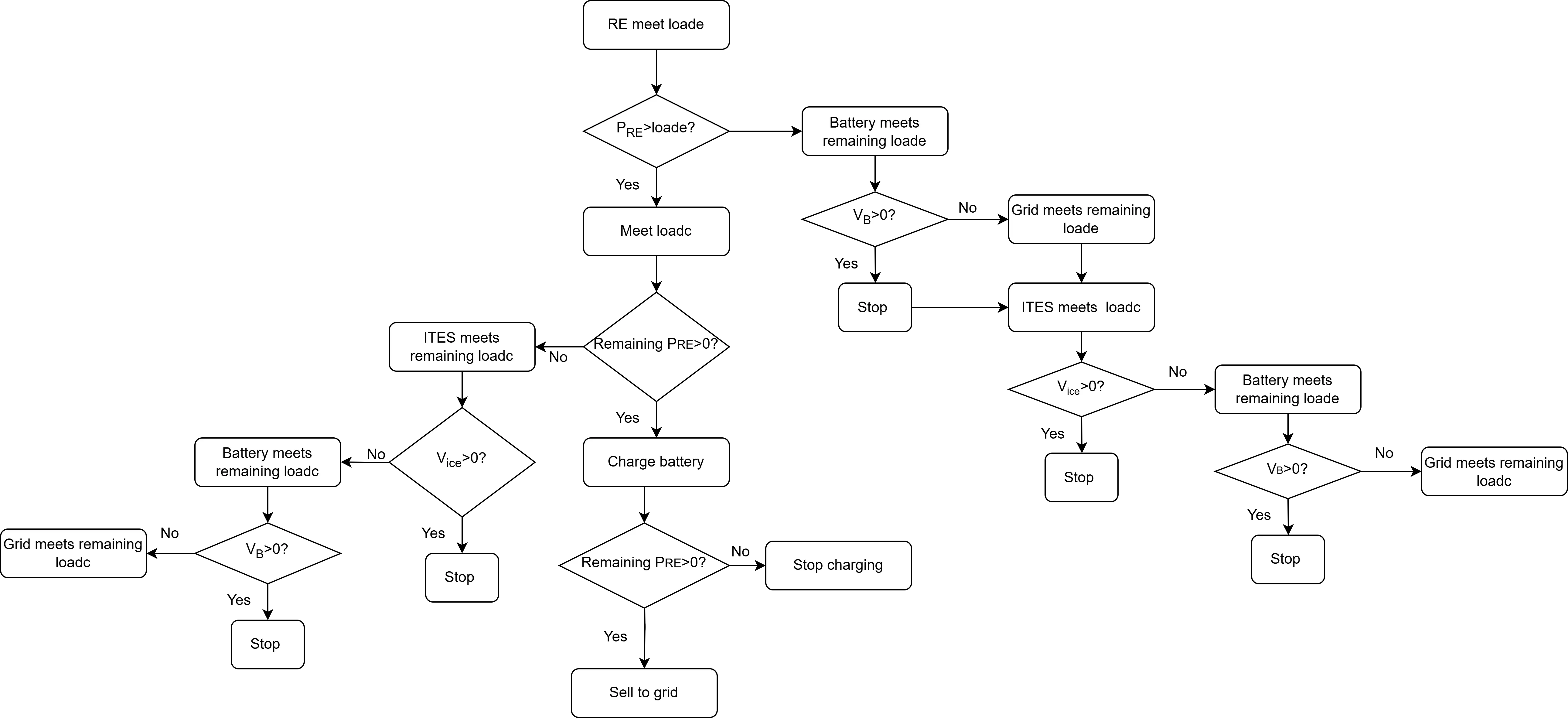
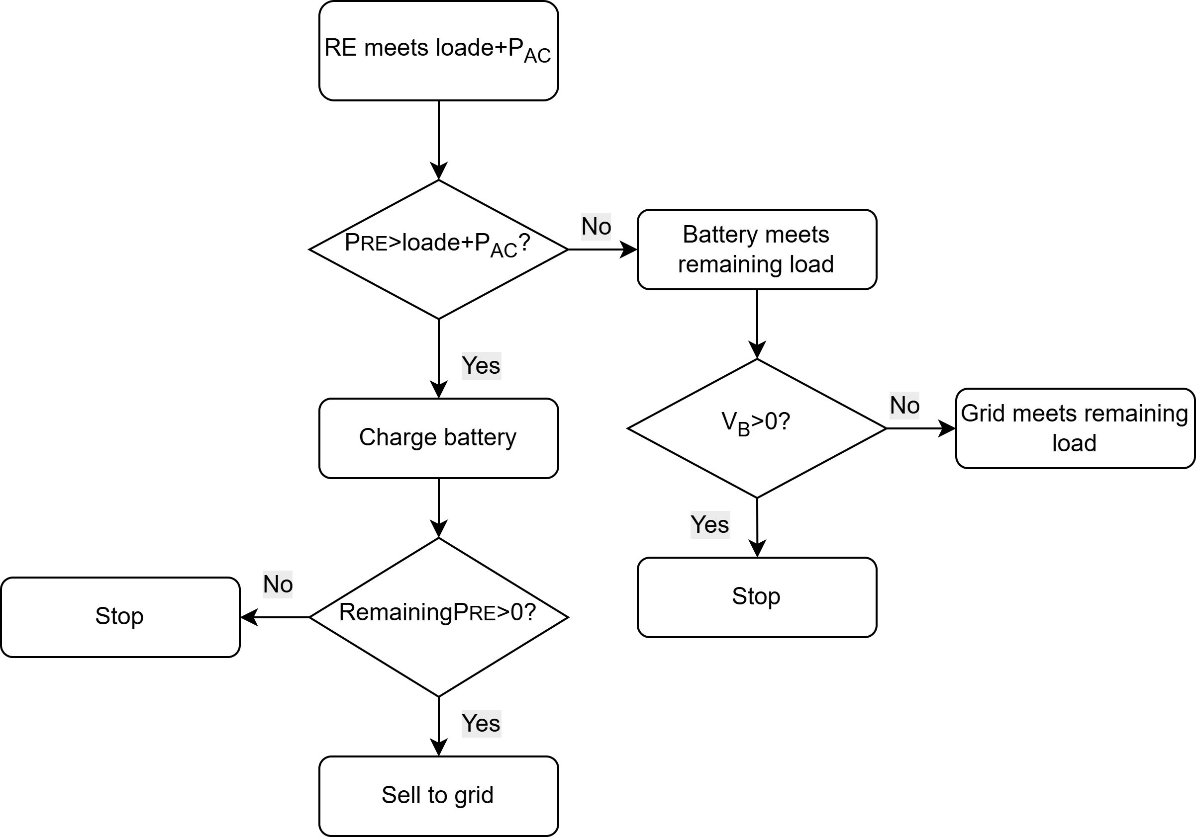
The operational logic is detailed in Figure 2 and Figure 3. Solar energy and wind energy are converted into electricity by PV and wind turbines, which primarily supplies building electric loads. Excess electricity either charges the battery or powers the dual-duty chillers to generate cooling energy. When RE generation exceeds the total demand of electric loads and battery storage capacity, surplus electricity is fed back into the grid. If the RE output is insufficient, the battery is discharged first to compensate for the shortfall. In cases where battery storage capacity is inadequate, electricity is purchased from the grid.
During the cooling season (April to October), the ITES operates in ice charging mode at night when the electricity price is low. The dual-duty chillers convert electrical energy into stored cooling energy. During the daytime, when the electricity price is high, it switches to ice discharging mode, prioritizing the release of stored cooling energy to meet cooling loads. If the ice storage capacity is insufficient to cover cooling demand, the system automatically activates the chillers to provide supplementary cooling. Notably, when RE generation exceeds instantaneous electric load requirements, the system prioritizes utilizing excess RE electricity to power the chillers for real-time cooling load. This mechanism reduces cooling costs during high-price periods while enhancing RE utilization efficiency.
Water pumps, as core components of the refrigerant circulation system, ensure efficient cooling energy transfer among chillers, ITES, and cooling loads. The power grid is a backup energy source, which ensures operational reliability in the system.
2.2. Modeling of IES Devices
This section aims to simulate energy flow dynamics within IES. The modeling comprises: output prediction modeling using LSTM for PV and wind turbines, and the establishment of physics-based mathematical models for equipment, such as chillers, ESSs, with particular attention to the modeling of ice storage devices incorporating nonlinear melting rate curves.
2.2.1. LSTM-Based Renewable Energy Prediction
As a specialized recurrent neural network architecture, the Long Short-Term Memory (LSTM) [37] network is employed in this study for RE generation forecasting due to its exceptional capability in modeling temporal dependencies and processing nonlinear sequential data. A simplified schematic diagram of the LSTM architecture is provided in Figure 4 to illustrate its operational principles. Compared to conventional Recurrent Neural Networks (RNNs), LSTM overcomes the vanishing gradient problem via its gating mechanisms [38], effectively capturing long-term dependencies in historical meteorological data and RE generation records. This advantage is particularly critical for RE forecasting tasks, as RE output exhibits pronounced diurnal and seasonal fluctuations influenced by meteorological factors such as solar irradiance, humidity, and wind speed [12].
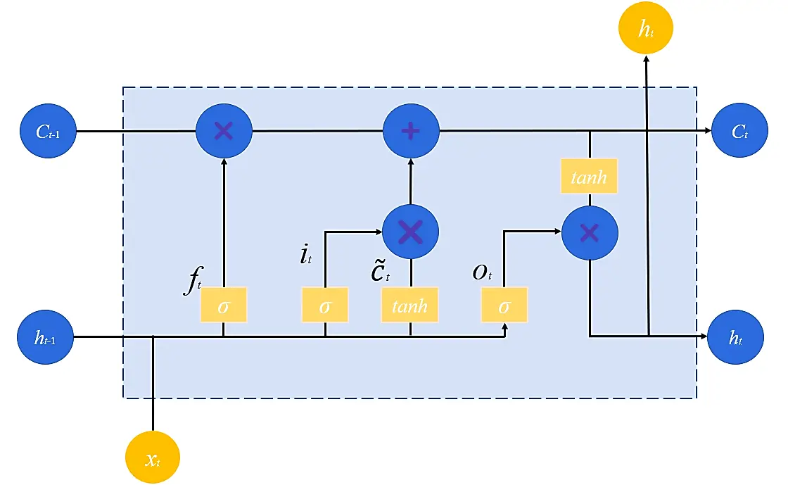
The LSTM unit’s core architecture consists of a cell state and three gating mechanisms (forget gate, input gate, output gate). Each unit processes three input parameters: the previous cell state Ct−1, current input xt, and hidden state ht−1.
The cell state serves as the primary information pathway, enabling direct temporal information propagation. The three gating mechanisms, implemented via sigmoid activation functions (yielding outputs between 0 and 1) and dot product operations, collectively regulate information flow by controlling the elimination of irrelevant information, the incorporation of relevant information, and the generation of the current output.
In this study, the LSTM model is designed to map historical time-series data to future power generation forecasts. Detailed descriptions of input data sources and prediction results are systematically addressed in the Case study section.
2.2.2. Cooling System Modelling
Chillers serve as the core refrigeration equipment in central cooling systems. Their energy consumption is strongly correlated with cooling capacity, operational efficiency, and part load ratio (PLR). The rated parameters of the dual-duty chiller model adopted in this study are listed in Table 1.
Table 1. Chiller rated parameters.
|
No. |
Power (kW) |
COP |
Cooling Capacity (kW) |
|---|---|---|---|
|
1 |
245 |
6.14 |
1502 |
|
2 |
664 |
5.82 |
3868 |
|
3 |
664 |
5.82 |
3868 |
The chiller model is developed using a multivariate gray-box modeling approach [33]. This model achieves high prediction accuracy for key operational parameters, including evaporating temperature, condensing temperature, and coefficient of performance (COP).
|
```latex\mathrm{C}\mathrm{O}\mathrm{P}=\frac{r}{\left(\frac{{t}_{c}+273.15}{{t}_{e}+273.15}-1\right)r+{a}_{1}\frac{{t}_{c}+273.15}{{t}_{e}+273.15}-{a}_{2}}``` |
(1) |
|
```latexr=\frac{{Q}_{e}}{Q}``` |
(2) |
|
```latex{t}_{e}={t}_{w,e,E}-\frac{{Q}_{e}}{{F}_{e}\left({G}_{w,e}\right)}``` |
(3) |
|
```latex{t}_{c}={t}_{w,c,E}+\frac{{Q}_{c}}{{F}_{c}\left({G}_{w,c}\right)}``` |
(4) |
|
```latex{P}_{chiller}=\frac{{Q}_{e}}{COP}``` |
(5) |
|
```latex{F}_{c}\left({G}_{w,c}\right)={a}_{3}\cdot {{G}_{w,c}}^{2}+{a}_{4}\cdot {G}_{w,c}+{a}_{5}``` |
(6) |
|
```latex{F}_{e}\left({G}_{w,e}\right)={a}_{6}\cdot{{G}_{w,e}}^{2}+{a}_{7}\cdot {G}_{w,e}+{a}_{8}``` |
(7) |
where r is the real-time load ratio of the chiller. tc and te represent the condensing temperature and evaporating temperature, respectively, °C. Qc and Qe are the real-time cooling capacity and real-time condensing heat output, respectively, kW. tw,e,E and tw,c,E indicate the chilled water inlet temperature and cooling water outlet temperature, respectively, °C. Gw,c and Gw,e correspond to the cooling water mass flow rate and chilled water mass flow rate, respectively, kg/s. F(Gw,c) and F(Gw,c) are empirical functions dependent on Gw,c and Gw,e, respectively. Coefficients a1 to a8 are fitting parameters determined experimentally using measured data of evaporating temperature, condensing temperature, chilled and cooling water flow rates, and inlet and outlet water temperatures.
Water pumps in central cooling systems are primarily utilized to circulate cooling water or chilled water to critical components such as cooling towers and chillers, thereby maintaining the system’s operational cycle. The rated parameters of the pumps in this system are summarized in Table 2.
Table 2. Pumps rated parameters.
|
Rated Parameters |
Chilled Pump1 |
Chilled Pump2 |
Cooling Pump1 |
Cooling Pump2 |
|---|---|---|---|---|
|
Flow rate (m3/h) |
730 |
280 |
865 |
350 |
|
Power (kW) |
110 |
45 |
90 |
37 |
|
Pressure (m) |
40 |
40 |
25 |
25 |
|
Frequency (Hz) |
50 |
50 |
50 |
50 |
The energy consumption of chilled water pumps and cooling water pumps is predominantly governed by their flow rates, with the corresponding energy consumption models explicitly formulated in Equation (8) and Equation (9).
|
```latex{P}_{c}={b}_{1}\cdot {{G}_{w,c}}^{2}+{b}_{2}\cdot {G}_{w,c}+{b}_{3}``` |
(8) |
|
```latex{P}_{e}={b}_{4}\cdot {{G}_{w,e}}^{2}+{b}_{5}\cdot {G}_{w,e}+{b}_{6}``` |
(9) |
where Pc and Pe are the power consumption of the cooling water pump and chilled water pump, respectively. b1~b6 represent the fitting coefficients for the pump models.
Cooling towers serve as the critical component in the heat rejection process of central cooling systems. The rated parameters of the cooling towers in this system are summarized in Table 3.
Table 3. Cooling Tower rated parameters.
|
Rated Parameters |
Value |
Unit |
|---|---|---|
|
Rated power |
51 |
kW |
|
Cooling capacity |
2326 |
kW |
|
Water flow rate |
400 |
m3/h |
The energy consumption model of cooling towers is similar to that of water pumps. It is developed based on their actual operating frequency, as suggested by existing literature. The corresponding energy consumption is expressed as shown in Equation (10).
|
```latex{P}_{co}={e}_{0}\cdot {f}^{3}+{e}_{1}\cdot {f}^{2}+{e}_{2}\cdot f+{e}_{3}``` |
(10) |
where Pco is the real-time power consumption of the cooling tower, f represents its operating frequency.
The model parameters for various components of the central cooling system were determined through experimental fitting and existing literature review, as listed in Table 4.
Table 4. Model parameters.
|
Model Parameters |
Value |
|---|---|
|
a1 |
−0.41527 |
|
a2 |
−0.49308 |
|
a3 |
−0.00521 |
|
a4 |
2.88287 |
|
a5 |
13.45778 |
|
a6 |
−0.01786 |
|
a7 |
4.96740 |
|
a8 |
8.52341 |
|
b1 |
−0.02668 |
|
b2 |
6.35890 |
|
b3 |
−4.33009 |
|
b4 |
−0.00268 |
|
b5 |
1.03823 |
|
b6 |
−0.20544 |
|
e0 |
0.00000381 |
|
e1 |
0.0001815 |
|
e2 |
−0.0064332 |
|
e3 |
0.091875 |
2.2.3. Battery
This paper utilizes the Deli NP100-12UPS model of storage battery, which is a 12 V, 100 Ah lead-acid battery. When there is renewable electricity, the excess energy is stored in the battery. When the renewable electricity is insufficient to meet the load demand, the stored energy in the battery is discharged.
The state of charge (SOC) is commonly used to represent the charging and discharging process of a battery.
Charging:
|
```latexSOC\left(t\right)=SOC\left(t-\mathrm{\Delta }t\right)+\frac{{P}_{bat}{\eta }_{b}\mathrm{\Delta }t}{{N}_{bat}}``` |
(11) |
Discharging:
|
```latexSOC\left(t\right)=SOC\left(t-\mathrm{\Delta }t\right)+\frac{{P}_{bat}\mathrm{\Delta }t}{{N}_{bat}{\eta }_{b}}``` |
(12) |
where Δt is the time duration for charge or discharge. Pbat is the charge and discharge power (positive value is charge, while negative value is discharge). ηb is the charge and discharge efficiency, which is 0.95 in this paper. Nbat is the battery capacity.
2.2.4. Ice Tank
As the cooling energy storage device in the integrated energy system, the ice storage tank enables peak shaving and valley filling. By leveraging time-of-use electricity pricing strategies, it stores cooling energy via ice formation during off-peak nighttime hours and releases stored energy during daytime peak periods. This operational strategy significantly reduces cooling costs during high-tariff intervals and alleviates grid load pressure [39].
Under ice storage mode, the ice storage rate can be considered constant [40]. The energy conversion efficiency from the chiller to the ice storage is influenced by losses in the distribution network and the operational characteristics of the ice storage equipment. The real-time ice storage capacity is expressed as:
|
```latex{Q}_{i}=\eta \cdot\sum\nolimits _{n=1}^{N}\sum\nolimits _{t={t}_{0}}^{{t}_{k}}{PLR}_{n}\left(t\right)\cdot{Q}_{n,cap}\left(t\right)``` |
(13) |
where $$\eta$$ is the cooling capacity conversion efficiency, set as 0.96. N represents the number of ice-making units. t0 and tk are the start and end times of the ice-making cycle, respectively. $${PLR}_{n}\left(t\right)\,$$indicates the partial load ratio of the n-th ice-making unit at time t. $${Q}_{n,cap}\,$$is the rated cooling capacity of the n-th ice-making unit, kW.
The ice melting rate is time-varying. In ice storage systems, the ice gradually melts inward from the outer layer of the storage tank. The thermal resistance of the ice-water mixture increases with melting duration, leading to a decay in melting rate, as depicted in the Figure 5. Studies [41] have demonstrated that the maximum instantaneous melting capacity during this process is a function of the remaining ice volume in the storage device.
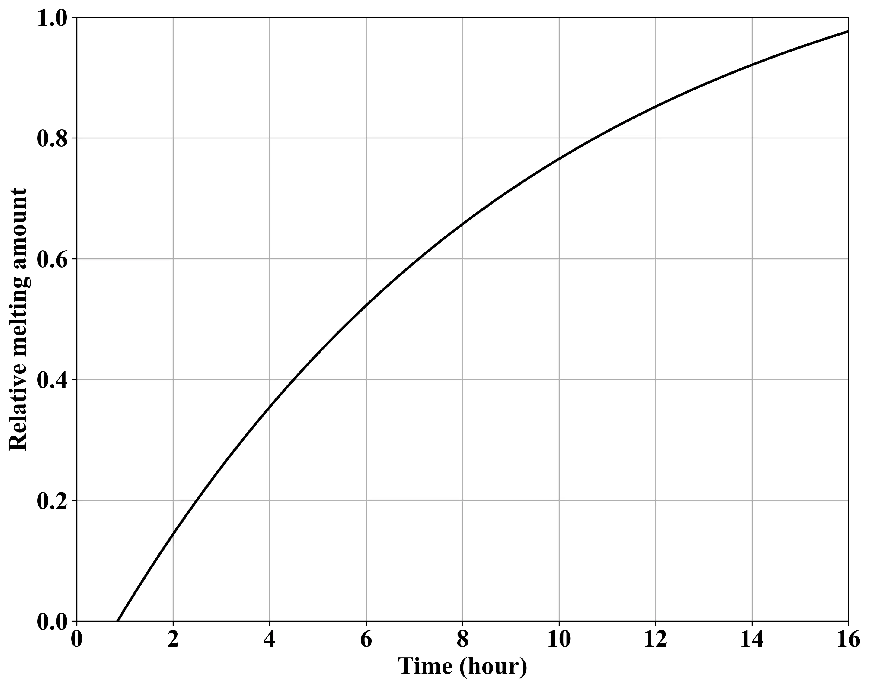
At time t, the maximum releasable cooling capacity of the ice storage tank is constrained by the residual ice volume and the instantaneous melting rate. The melting rate is formulated in Equation (14) and Equation (15). This nonlinear melting model has been experimentally validated in Ref. [41].
|
```latex{\epsilon }_{\beta }=0.1463\cdot\left(1.1992-\beta \right)/1.3176``` |
(14) |
|
```latex\beta =1.1992-1.3176\cdot {e}^{-1.11106t}``` |
(15) |
where $$\beta$$ is the percentage of melted ice relative to the total ice storage capacity.
The maximum ice melting capacity of the ice storage tank at time t is:
|
```latex{Q}_{m}=\frac{{Q}_{it}\cdot {\epsilon }_{\beta }}{H}``` |
(16) |
where Qit is the total capacity of the ice tank. H is the ice melting time.
2.3. Optimization Problem
2.3.1. Objective Functions
In the design of IES, this study considers the daily operating cost (Cost), CO2 emission reduction rate (CDERR), and renewable energy utilization rate (RU) as objectives for optimizing the system from the perspectives of economy, environment, and energy.
|
```latex\left\{ \begin{array}{l} min(\mathit{Cost}) \\ max(\mathit{CDERR}) \\ max(\mathit{RU}) \end{array} \right.``` |
(17) |
The daily operating cost is expressed as:
|
```latexCost=\frac{LCC}{N*365}``` |
(18) |
LCC is the life cycle cost [42]. N is the life span of the system, which is 20 years in this study. It should be noted that the current economic assessment assumes constant component efficiency over the system lifetime and fixed energy prices.
|
$$LCC=ICC-\sum _{n=1}^{N}\frac{{d}_{n}}{{\left(1+i\right)}^{n}}tr+\sum _{n=1}^{N}\frac{{a}_{n}}{{\left(1+i\right)}^{n}}\left(1-tr\right)+\sum _{r=1}^{R}\frac{{ICC}_{n}}{{\left(1+i\right)}^{r{l}_{c}}}\left(1-tr\right)-\frac{s}{{\left(1+i\right)}^{N}}$$ |
(19) |
where ICC is the initial capital cost of the system (US$). i represents the interest rate, set at 7% in this study. dn is the annual depreciation (US$). tr indicates the tax rate, defined as 5% in this study. an is the annual maintenance and operational costs. R refers to the number of equipment replacements over the system lifecycle. ICCn signifies the replacement cost of the n-th component. lc is the lifecycle of the n-th replaced component. s stands for the system salvage value.
|
```latexICC={N}_{PV}{C}_{PV}+{N}_{WT}{C}_{WT}+{N}_{B}{C}_{B}+{N}_{ICE}{C}_{ICE}``` |
(20) |
where NPV and NWT are the number of installed PV panels and Wind turbines in the system, respectively. NB and NICE represent the capacity of the battery storage and ice storage tank, respectively (kWh); C is the unit cost of the equipment, defined as the price per unit quantity or capacity.
|
```latexCDERR=\frac{{m}_{C{O}_{2},tra}-{m}_{C{O}_{2},new}}{{m}_{C{O}_{2},tra}}``` |
(21) |
where mCO2,tra and mCO2,new are the CO2 emission in the tradition energy supply mode and the proposed method in this paper.
The traditional energy supply mode typically generates electricity through coal combustion. The production of 1 kWh of electricity requires the consumption of 360 g of standard coal.
|
```latex{m}_{C{O}_{2},tra}=0.36{u}_{C{O}_{2}}sum\left({E}_{load}+{E}_{AC}\right)``` |
(22) |
|
```latex{m}_{C{O}_{2},new}=0.36{u}_{C{O}_{2}}sum\left({E}_{grid,in}\right)``` |
(23) |
where uCO2 is the CO2 emission of standard coal. sum(Eload) and sum(EAC) are the total electric load and the total power of the air conditioning system. Sum(Egrid,in) is the electricity purchased from the grid.
|
```latexRU=1-\frac{sum\left({E}_{grid,out}\right)}{sum\left({P}_{RE}\right)}``` |
(24) |
where sum(Egrid,out) is the electricity sold to the grid. $$sum\left({P}_{RE}\right)$$ is the total RE power.
2.3.2. Decision Variables
Based on the composition and operational strategies of the IES, this optimization problem requires the determination of four key variables: $${N}_{PV}{,N}_{WT},{N}_{B},{N}_{ICE}$$. NB and NICE represent the energy storage capacity of the system. It should be noted that this optimization focuses solely on the design capacities of the system components. The operational dispatch follows fixed rule-based strategies as described in Section 2.1 and Figure 2 and Figure 3.
2.3.3. Constraints
The constraints of an IES can be divided into equality constraints and inequality constraints.
Equality Constraints
The equality constraints primarily refer to the operational requirements and energy balance constraints of the system. The following equation gives the energy balance constraint at each time:
Electricity balance:
|
```latexE_{pv,i} + E_{wt,i} = E_{load,i} + E_{AC} + d(E_{bat})_i + E_{grid,out,i}``` |
(25) |
where d(Ebat)i is the battery electricity change at time period i.
Cooling balance:
Ice storage period:
|
```latex{Q}_{AC,i}={Q}_{storage,i}+{Q}_{load,i}``` |
(26) |
Ice melting period:
|
```latex{Q}_{load,i}={Q}_{storage,i}+{Q}_{AC,i}``` |
(27) |
Inequality Constraints
The inequality constraints primarily include constraints on equipment capacity, constraints on equipment power, constraints on states of equipment such as SOC of battery.
|
```latex{N}_{PV}^{min}\le {N}_{PV}\le {N}_{PV}^{max}``` |
(28) |
|
```latex{N}_{WT}^{min}\le {N}_{WT}\le {N}_{WT}^{max}``` |
(29) |
|
```latex{N}_{B}^{min}\le {N}_{B}\le {N}_{B}^{max}``` |
(30) |
|
```latex{N}_{ICE}^{min}\le {N}_{ICE}\le {N}_{ICE}^{max}``` |
(31) |
|
```latex0\le {Q}_{ICE,STO}\le {Q}_{ICE,STO}^{max}``` |
(32) |
|
```latex0\le SOC\left(t\right)\le 1``` |
(33) |
2.4. Optimization Solution
2.4.1. Overview of PPO
As a prominent reinforcement learning algorithm, PPO is designed to optimize policies by iteratively updating them within a trust region, ensuring stable and efficient training [43]. Unlike traditional policy gradient methods, PPO introduces a clipped surrogate objective function to limit policy updates, preventing drastic changes that could destabilize learning. This mechanism balances exploration and exploitation by constraining the policy’s deviation from its previous version. The core innovation of PPO lies in its clipped surrogate objective:
|
```latexL^{CLIP}(\theta) = \widehat{E}_t\big[\min\big(r_t(\theta)\widehat{A_t},\,clip\big(r_t(\theta),\,1-\epsilon,\,1+\epsilon\big)\widehat{A_t}\big)\big]``` |
(34) |
|
```latex{r}_{t}\left(\theta \right)=\frac{{\pi }_{\theta }\left({a}_{t}\mid {s}_{t}\right)}{{\pi }_{\theta old}\left({a}_{t}\mid {s}_{t}\right)}``` |
(35) |
where $$\widehat{A_t}$$ is the estimated advantage function at timestep t. $${r}_{t}\left(\theta \right)$$ is the probability ratio between the new and old policies. $$ϵ$$ defines the clipping range to prevent excessively large policy updates.
The Critic network in PPO estimates the state-value function, which is trained to minimize the mean squared error (MSE) between predicted and target values:
|
```latexL^{VALUE}(\phi) = \widehat{E}_t\left[\left(V_\phi(s_t) - \widehat{R}_t\right)^2\right]``` |
(36) |
where $$\widehat{R}_t$$ is the discounted cumulative reward calculated using Generalized Advantage Estimation (GAE). The advantage function $$\widehat{A}_t$$ is derived as:
|
```latex\hat{A}_t = \hat{R}_t - V_\phi(s_t)``` |
(37) |
PPO employs an Actor-Critic architecture. The Actor updates the policy $${\pi }_{\theta }\left(a\mid s\right)$$ using the clipped objective $${L}^{CLIP}$$, and the Critic updates the value function $${V}_{\phi }\left(s\right)$$ via $${L}^{VALUE}$$, providing a baseline to reduce variance in policy gradients. This dual-network design enables efficient exploration-exploitation trade-offs while maintaining training stability.
PPO’s simplicity and robustness enable it to be widely applied in single-objective optimization tasks, such as robotic control and game playing. However, its reliance on a single reward function limits its adaptability to complex scenarios requiring multi-objective trade-offs (e.g., balancing energy efficiency, cost, and environmental impact). To address this, this study extends PPO to a multi-objective framework, addressing challenges in reward shaping and optimization stability through adaptive mechanisms.
2.4.2. MOPPO
Traditional PPO employs a scalar reward function $$r(s,a) \in \hat{R}$$ to direct the agent toward optimizing a single objective, where policy gradient updates are dominated by the value function of that singular goal. In contrast, complex scenarios such as IES necessitate the simultaneous optimization of multi-dimensional objectives (e.g., economic efficiency, environmental sustainability, and energy utilization), which inherently constitutes a multi-objective optimization problem. To address this, the proposed framework confronts two critical challenges:
-
Reward Dimensionality Expansion: Multi-Objective Reinforcement Learning (MORL) redefines rewards as a vector r(s,a) = [r1, r2, r3]T∈$$\hat{R}_d\,$$where each dimension corresponds to a distinct objective (e.g., cost minimization, CO2 reduction, and photovoltaic utilization).
-
Pareto Optimality: Optimization must generate a Pareto front (PF), representing a set of non-dominated trade-off solutions in the objective space.
To address these challenges, this study proposes a MOPPO framework, as outlined in Algorithm 1. Key innovations include:
Vectorized Reward Processing: Extends the scalar reward function in traditional single-objective reinforcement learning to a multi-dimensional vector form, explicitly preserving trade-offs among objectives.
| Algorithm 1 Multi-Objective Proximal Policy Optimization | |
|---|---|
| 1 | Initialize: Policy network πθ, value network Vϕ, Pareto frontier PF ←, state normalizer Ns, reward normalizer Nr |
| 2 | for episode = 1 to Nmax do |
| 3 | Collect trajectory D = {(st, at, rt)} via πθ |
| 4 | Update Ns with states, Nr with rewards |
| 5 | for step t = 1 to T in episode do |
| 6 | Extract multi-objective reward vector $$\mathrm{rt}=\begin{bmatrix}r_t^1&,...,\mathrm{r}_t^M&\end{bmatrix}$$ |
| 7 | if rt non-dominated by PF then |
| 8 | Remove solutions in PF dominated by rt |
| 9 | PF ← PF ∪ {rt} |
| 10 | end if |
| 11 | end for |
| 12 | for objective m = 1 to M do |
| 13 | Compute $$A^m\quad\leftarrow\mathrm{GAE}(\lambda)$$ using Vϕ |
| 14 | end for |
| 15 | Randomly select k solutions {Rp} from PF |
| 16 | Compute advantage direction: $$\bar{A}\leftarrow1/k\sum\nolimits_{p=1}^k(R_p-V_\phi(s))\cdot A$$ |
| 17 | Update policy using Ā as advantage signal |
| 18 | for epoch = 1 to K do |
| 19 | Compute value target: Vtarget ← Vϕ(s) + Ā |
| 20 | Update value network: $$\min\phi\parallel V\phi(s)-Vtarget\parallel_2^2$$ |
| 21 | Compute ratio ρ(θ) ← πθ(a|s) / πold(a|s) |
| 22 | Calculate loss Lclip ← E[min(y, clip(ρ, 1 ± ε)Ā)] |
| 23 | Compute entropy Lent ← H(πθ) |
| 24 | Update θ ← Adam(∇θ(Lclip + 0.01Lent)) |
| 25 | end for |
| 26 | end for |
Pareto Policy Selection: At the end of each training episode, non-dominated sorting is applied to state-action trajectories within the trajectory buffer to dynamically generate the current Pareto front. The frontier solution set directly guides policy network updates, ensuring balanced convergence across competing objectives.
In the design of IES, this study redefines the core elements of the reinforcement learning framework to accommodate multi-objective optimization:
State Space: The state vector s = [s1, s2, s3, s4], where:
s1: installed capacity of PV (m2). s2: installed capacity of wind turbine (number of units). s3: battery storage capacity (kWh). s4: ice storage tank capacity (kWh). Each state variable is normalized to the range [0, 1] based on its predefined upper and lower bounds (as given in Section 2.3.3, Constraints).
Action Space: The action vector shares the same dimensionality as the state vector. Each dimension ai governs the directional adjustment and magnitude of the corresponding state parameter si, thereby transforming the continuous design optimization problem into a learnable policy search process.
Reward: The reward vector is defined as r = [r1, r2, r3]T, where:
r1: −Cost (negative daily operating cost, to be minimized). r2: CDERR (CO2 emission reduction rate, to be maximized). r3: RU (renewable energy utilization rate, to be maximized).
According to Algorithm 1, the workflow of MOPPO can be divided into four stages:
- (1)
-
Multi-objective Reward Processing and Pareto Front Maintenance (Lines 4–7): At every step of episode, the multi-dimensional reward vector rt = [r1, r2, r3] is extracted. To avoid dominance by any single objective during optimization due to differences in units and scales, all reward components are normalized to a comparable numerical interval. Specifically, each reward component ri (i.e., Cost, CDERR, RU) is normalized linearly to the range [0, 1] based on the minimum and maximum values observed in the current Pareto front. This ensures that no objective inherently dominates the policy update because of its absolute magnitude. The normalized reward vector is then used for non-dominated sorting and advantage computation. The PF is dynamically updated based on non-dominated criteria: if rt is not dominated by any solution in PF, it is added to PF, while existing solutions dominated by rt are removed, which ensures PF consistently represents the optimal trade-off solutions. Thus, at each episode step, the reward vector of the current state-action trajectory is compared against all stored solutions in the Pareto set. Dominance is determined using standard Pareto dominance rules (i.e., solution A dominates solution B if A is no worse than B in all objectives and strictly better in at least one). This mechanism guarantees that only non-dominated solutions are retained, and the frontier evolves monotonically toward the true Pareto front.
- (2)
-
Advantage Computation (Lines 8–10): Instead of a scalar advantage, we compute a global advantage direction. k reference solutions {Rp}are selected from PF. The advantage is then calculated as $$\bar{A}=\frac{1}{k}\sum \left({R}_{p}-{V}_{\mathrm{\phi }}\left(s\right)\right)\cdot A$$, where $$\bar{A}$$ is the original advantage from the critic. This projects the multi-objective reward differences into a scalar advantage that reflects the overall improvement direction toward the Pareto front.
- (3)
-
Policy Network Optimization (Lines 11–15): The clipped surrogate objective of PPO is adapted to use this $$\bar{A}$$
```latexL^{CLIP}(\theta)=\hat{E}[\min{(r_t(\theta)\bar{A},clip(r_t(\theta),1-\epsilon,1+\epsilon)\bar{A})}]```
(38)
An entropy regularization term Lent = H(πθ) is introduced to enhance exploration.
- (4)
-
Critic Network Training (Lines 16–19): For M optimization objectives, critic networks {Vϕm} are trained by minimizing the mean squared error (MSE), which provides accurate state-value estimates for each objective, enabling the actor to learn a policy that balances all objectives simultaneously.
2.4.3. MOPPO Evaluation
DTLZ2 and DTLZ5 are classic multi-objective optimization benchmarks designed to evaluate algorithmic performance in high-dimensional objective spaces, focusing on convergence, distribution characteristics, and adaptability to complex geometric structures. Specifically:
DTLZ2: Its PF is a segment of a hypersphere, serving to assess global convergence in uniformly distributed objective spaces. The mathematical formulation of DTLZ2 is given by:
|
$$Minimize\begin{cases}f_1(x)=\left(1+g(x)\right)\cos\left(\frac{x_1\pi}{2}\right)\cos\left(\frac{x_2\pi}{2}\right)...\cos\left(\frac{x_{M-2}\pi}{2}\right)\cos\left(\frac{x_{M-1}\pi}{2}\right)\\f_2(x)=\left(1+g(x)\right)\cos\left(\frac{x_1\pi}{2}\right)\cos\left(\frac{x_2\pi}{2}\right)...\cos\left(\frac{x_{M-2}\pi}{2}\right)\sin\left(\frac{x_{M-1}\pi}{2}\right)\\ \,\,\,\,\,\,\,\,\,\,\,\,\,\,\,f_3(x)=\left(1+g(x)\right)\cos\left(\frac{x_1\pi}{2}\right)\cos\left(\frac{x_2\pi}{2}\right)...\sin\left(\frac{x_{M-2}\pi}{2}\right)\\\,\,\,\,\,\,\,\,\,\,\,\,\,\,\,\,\,\,\,\,\,\,\,\,\,\,\,\,\,\,\,\,\,\,\,\,\,\,\,\,\,\,\,\,\,\,\,\,\,\,\,\,\,\,\,\,\,\,\,\,\,\,\,\,\,\,\,\,\,\,\,\,\,\,\,\vdots\\\,\,\,\,\,\,\,\,\,\,\,\,\,\,\,\,\,\,\,\,\,\,\,\,\,\,\,\,\,\,\,\,f_k(x)=\left(1+g(x)\right)\cos\left(\frac{x_1\pi}{2}\right)...\sin\left(\frac{x_{M-k+1}\pi}{2}\right)\\ \,\,\,\,\,\,\,\,\,\,\,\,\,\,\,\,\,\,\,\,\,\,\,\,\,\,\,\,\,\,\,\,\,\,\,\,\,\,\,\,\,\,\,\,\,\,\,\,\,\,\,\,\,\,\,\,\,\,\,\,\,\,\,\,\,\,\,\,\,\,\,\,\,\,\,\vdots\\\,\,\,\,\,\,\,\,\,\,\,\,\,\,\,\,\,\,\,\,\,\,\,\,\,\,\,\,\,\,\,\,\,\,\,\,\,\,\,\,\,\,\,\,\,\,\,f_M(x)=\left(1+g(x)\right)\sin\left(\frac{x_1\pi}{2}\right)&\end{cases}$$ |
(39) |
|
Subject to: $$0<{x}_{i}<1, \forall i=1, 2, \dots , n$$ |
(40) |
|
where: $$g\left(x\right)={\sum }_{i=M}^{n}{\left({x}_{i}-0.5\right)}^{2}$$ |
(41) |
DTLZ5: By introducing nonlinear variable correlations, it constructs a non-uniform PF to test solution uniformity and local search capability in geometrically complex scenarios. The mathematical formulation of DTLZ5 is given by:
|
```latexMinimize\begin{cases}f_1(x)=\left(1+g(x)\right)\cos\left(\frac{\theta_1\pi}{2}\right)\cos\left(\frac{\theta_2\pi}{2}\right)...\cos\left(\frac{\theta_{M-1}\pi}{2}\right)\\f_2(x)=\left(1+g(x)\right)\cos\left(\frac{\theta_1\pi}{2}\right)\cos\left(\frac{\theta_2\pi}{2}\right)...\sin\left(\frac{\theta_{M-1}\pi}{2}\right)\\ \,\,\,\,\,\,\,\,\,\,\,\,\,\,\,\,\,\,\,\,\,\,\,\,\,\,\,\,\,\,\,\,\,\,\,\,\,\,\,\,\,\,\,\,\,\,\,\,\,\,\,\,\,\,\,\,\,\,\,\,\,\vdots\\ \,\,\,\,\,\,\,\,\,\,\,\,\,\,\,\,\,\,\,\,\,\,\,\,\,\,\,\,\,\,\,\,\,\,\,\,\,\,\,\,\,\,\,\,\,\,\,\,\,\,\,\,\,\,\,\,\,\,\,\,\,\vdots\\ \,\,\,\,\,\,\,\,\,\,\,\,\,\,\,f_k(x)=\left(1+g(x)\right)\cos\left(\frac{\theta_1\pi}{2}\right)...\sin\left(\frac{\theta_{M-k+2}\pi}{2}\right)\\ \,\,\,\,\,\,\,\,\,\,\,\,\,\,\,\,\,\,\,\,\,\,\,\,\,\,\,\,\,\,\,\,\,\,\,\,\,\,\,\,\,\,\,\,\,\,\,\,\,\,\,\,\,\,\,\,\,\,\,\,\,\vdots\\ \,\,\,\,\,\,\,\,\,\,\,\,\,\,\,\,\,\,\,\,\,\,\,\,\,\,\,\,\,\,f_M(x)=\left(1+g(x)\right)\sin\left(\frac{\theta_1\pi}{2}\right)&&\end{cases}``` |
(42) |
|
Subject to: $$0<{x}_{i}<1, \forall i=1, 2,\dots ,n$$ |
(43) |
|
```latex\theta=\begin{cases}\,\,\,\,\,\,\frac{\pi}{4\left(1+g(x)\right)}\left(1+2g(x)x_i\right)i=1\\\frac{\pi}{4\left(1+g(x)\right)}\left(1+2g(x)x_i\right)i=2,3,...,n&\end{cases}``` |
(44) |
|
```latexg\left(x\right)={\sum }_{i=M}^{n}{\left({x}_{i}-0.5\right)}^{2}``` |
(45) |
The Inverted Generational Distance (IGD) is a multi-objective optimization performance metric that evaluates the distribution and convergence of solution sets by calculating the average Euclidean distance between the algorithm-derived solutions and the true Pareto front. A smaller IGD value indicates closer proximity to the true front and better distribution uniformity. The key parameter configurations for MOPPO, MOPSO, and MOSFO are shown in Table 5.
Table 5. Algorithm parameters.
|
Algorithm |
The Setting of the Relevant Parameters |
|---|---|
|
MOPPO |
Episode = 200, step = 10, boundary of action = [0, 1], gamma = 0.99 |
|
MOPSO |
MaxIt = 200, Pop = 50, ω= 0.5 |
|
MOSFO |
MaxIt = 200, Pop = 50, pollination rate = 0.1, mortality rate = 0.1 |
2.4.4. Decision-Making Method
It is noteworthy that the Pareto front inherently characterizes a fundamental attribute of multi-objective optimization problems: trade-offs exist among competing objectives, making it impossible to achieve optimal results for all of them. Consequently, no single solution absolutely dominates all others. To resolve this decision-making challenge, this study employs the Technique for Order Preference by Similarity to Ideal Solution (TOPSIS) for further refinement and ranking of the Pareto solution set.
The core concept of TOPSIS lies in constructing positive and negative ideal solutions within the multi-objective space, then measuring the Euclidean distance between each candidate solution and these reference points. The relative closeness derived from these distances serves as the metric for solution ranking. To eliminate dimensional heterogeneity among objectives, all objective values undergo normalization via linear scaling to the [0, 1] interval prior to distance computation. For the normalized value zij the j-th objective in the i-th solution, the following formulation applies:
|
```latexZ=\begin{cases}\frac{x_{ij}-x_j^{min}}{x_j^{max}-x_j^{min}}\\\frac{x_j^{max}-x_{ij}}{x_j^{max}-x_j^{min}}&\end{cases}``` |
(46) |
The positive ideal solution Z+ and negative ideal solution Z− are defined as the sets of maximum and minimum values across all normalized objectives, respectively. Subsequently, the Euclidean distances between the i-th solution and these ideal references are computed as follows [44]:
|
$${D}_{i}^{+}=\sqrt{\sum _{j=1}^{m}{\left({z}_{ij}-{z}_{j}^{+}\right)}^{2}}$$ |
(47) |
|
$${D}_{i}^{-}=\sqrt{\sum _{j=1}^{m}{\left({z}_{ij}-{z}_{j}^{-}\right)}^{2}}$$ |
(48) |
The relative closeness is expressed as follow:
|
```latex{C}_{i}=\frac{{D}_{i}^{-}}{{D}_{i}^{+}+{D}_{i}^{-}}``` |
(49) |
A Ci value closer to 1 indicates better solution performance.
3. Case Study
3.1. Meteorological and Load Analysis
The building electricity and cooling load data used in this study were obtained through an 8760-h annual dynamic simulation of an office building in Shanghai using EnergyPlus. The meteorological data, sourced from the Shanghai Typical Meteorological Year (TMY) file available at https://energyplus.net/weather (accessed on 8 October 2024), include hourly dry-bulb temperature, relative humidity, solar irradiance (direct and diffuse), and wind speed.
The annual solar radiation, temperature, as well as wind speed variation profiles are shown in Figure 6. It can be seen that the solar radiation is concentrated from late spring to summer, characterized by high intensity and long duration, while the temperature exhibits distinct seasonal fluctuations, with prolonged higher temperatures in summer and lower temperatures in winter. The annual wind speed variation indicates that the region possesses relatively abundant wind resources, demonstrating potential to develop and utilize wind energy for RE generation.
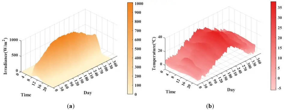
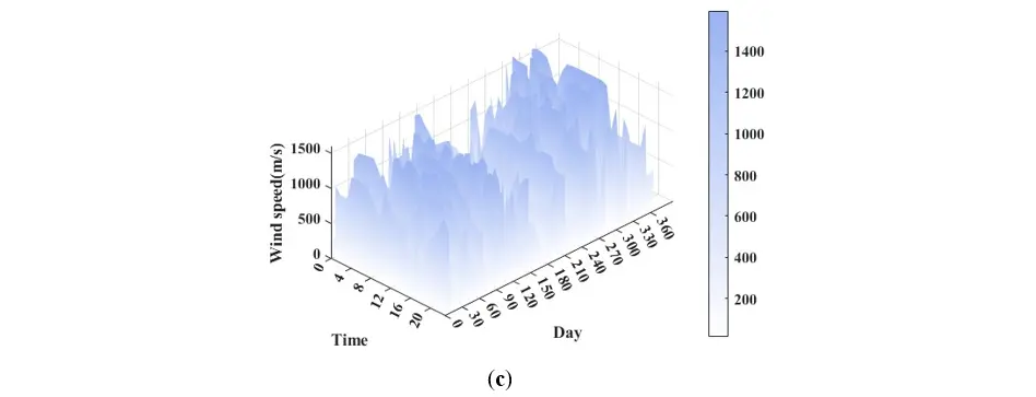
Figure 7 illustrates the hourly cooling and electricity load profiles across summer, transitional seasons, and winter. In summer, the cooling load peaks during daytime hours, particularly from noon to afternoon, driven by intensive cooling demand. Transitional seasons exhibit significantly lower cooling loads, with minor fluctuations concentrated around midday. In contrast, winter cooling demand is negligible, reflecting minimal refrigeration requirements. Meanwhile, the electricity load consistently demonstrates a dual-peak pattern (midday and evening) throughout all seasons. However, the magnitude and temporal characteristics of these peaks are strongly modulated by seasonal cooling load variations.
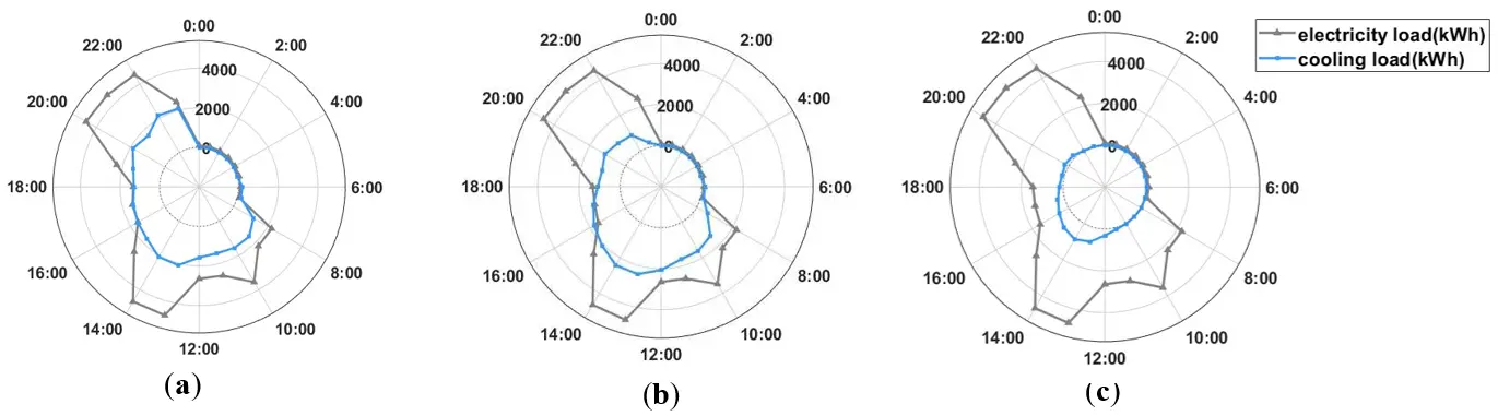
Figure 7. Typical-day load profiles of different seasons. (a) Summer; (b) Transitional seasons; (c) Winter.
3.2. Parameter Settings
The parameter configuration for this case study comprises equipment economic parameters, energy pricing parameters, and algorithmic parameters. The specifications for the first two are detailed in Table 6 and Table 7 [45], while the algorithmic parameters are given in Table 8.
Table 6. Economic parameters of each device.
|
Device |
Value |
|---|---|
|
PV |
1.05 $/W |
|
Wind turbine |
1.45 $/W |
|
Ice tank |
0.5 $/W |
|
Battery |
0.5 $/W |
Table 7. Time-of-use (TOU) Electricity Pricing Structure.
|
Period Type |
Time Range |
Value (US$) |
|---|---|---|
|
Peak |
8:00–23:00 |
0.086 |
|
Off Peak |
0:00–7:00 |
0.043 |
|
feed in tariff |
0:00–23:00 |
0.056 |
Table 8. MOPPO and LSTM parameters.
|
Item |
Value |
|
|---|---|---|
|
MOPPO |
Episode |
1000 |
|
Step of every episode |
2 |
|
|
Hidden Layer Dimension |
128 |
|
|
Actor Learning Rate |
0.0003 |
|
|
Critic Learning Rate |
0.00003 |
|
|
Discount Factor (γ) |
0.99 |
|
|
Clipping Epsilon (ε) |
0.2 |
|
|
GAE parameter (λ) |
0.95 |
|
|
Entropy coefficient |
0.01 |
|
|
LSTM |
Train |
80% |
|
Test |
20% |
|
|
Learning rate |
0.001 |
|
|
Batch size |
32 |
|
|
R2 (PV) |
0.89 |
|
|
RMSE (PV) |
6.83% |
|
|
R2 (wind) |
0.87 |
|
|
RMSE (wind) |
8.41% |
3.3. Wind and Solar Power Prediction Model
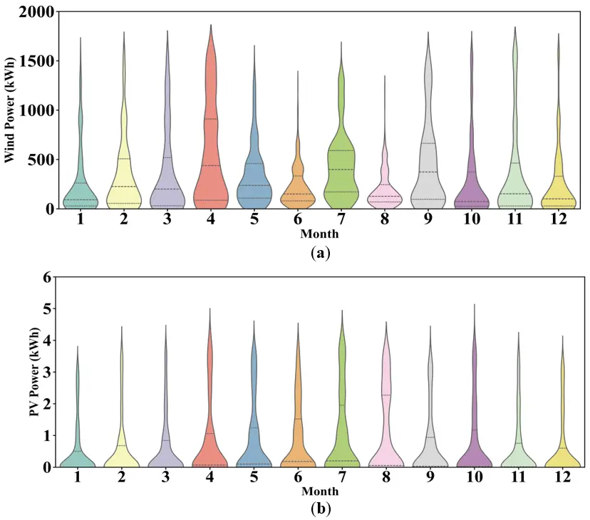
In this study, LSTM-based prediction models were developed for PV and wind power generation forecasting. The specifications of the components are provided in Table 9. The PV power model was trained using meteorological data and PV output records from the Alice Springs Solar Centre in Australia [46], with each PV unit having a rated capacity of 5.4 kW as the basic prediction unit, and was applied to estimate PV power generation in Shanghai. The wind power model was trained on wind speed and direction data from a wind farm in China [47], and was transferred to estimate wind power generation in Shanghai. This is under the assumption of similar PV and wind turbine characteristics. According to prior research by the author team [48,49], such model transfer methods based on physical similarity have been validated to be effective in cross-regional applications. The annual distributions of PV and wind power generation are illustrated in Figure 8.
Table 9. Rated Technical Parameters of PV Panels and Wind Turbines.
|
Device Type |
Parameter |
Value |
Unit |
|---|---|---|---|
|
PV |
Panel Type |
BP 3165 |
/ |
|
Panel Rateing |
165 |
W |
|
|
Panel Area |
1.26 |
m2 |
|
|
WT |
Turbine Type |
XE72 |
|
|
Capacity |
2000 |
kW |
|
|
Hub height |
65.0 |
m |
|
|
Rotor diameter |
70.7 |
m |
4. Results and Discussion
4.1. Comparison of Different Optimization Algorithms
This section presents a comprehensive performance evaluation of the proposed MOPPO algorithm, comparing it against state-of-the-art multi-objective optimization methods: Multi-Objective Particle Swarm Optimization (MOPSO) and Multi-Objective Sunflower Optimization (MOSFO). Two widely recognized multi-objective test functions (DTLZ2 and DTLZ5), together with the IGD, are adopted as the performance metrics to evaluate both distribution and convergence of the solution sets.
4.1.1. PF Analysis of MOPPO on Benchmark Problems
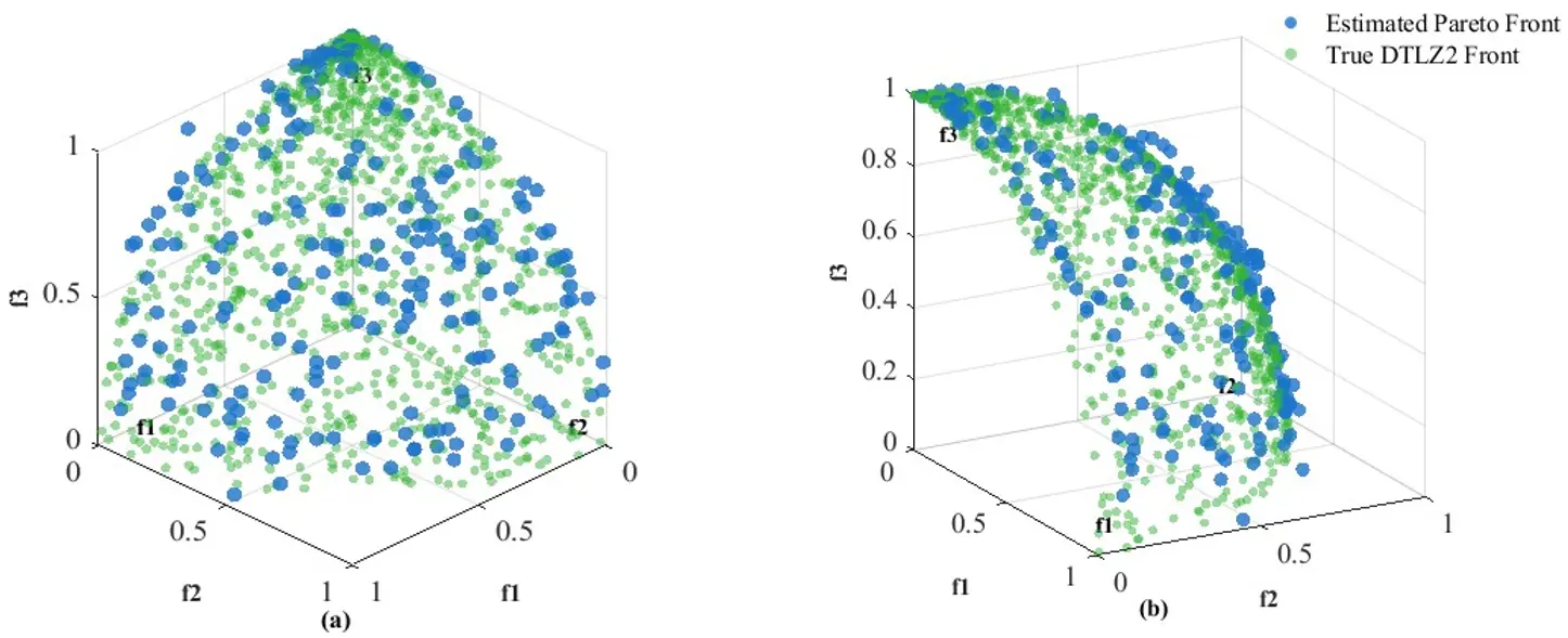
Figure 9 illustrates the three-dimensional comparison between the Pareto optimal solutions (blue points) generated by the MOPPO and the true PF (green points) for DTLZ2. The results show that MOPPO’s solution set closely aligns with the true PF surface and exhibits a uniform distribution along the objective axes (f1, f2, and f3), demonstrating its superior convergence and diversity preservation in balancing multi-objective conflicts.
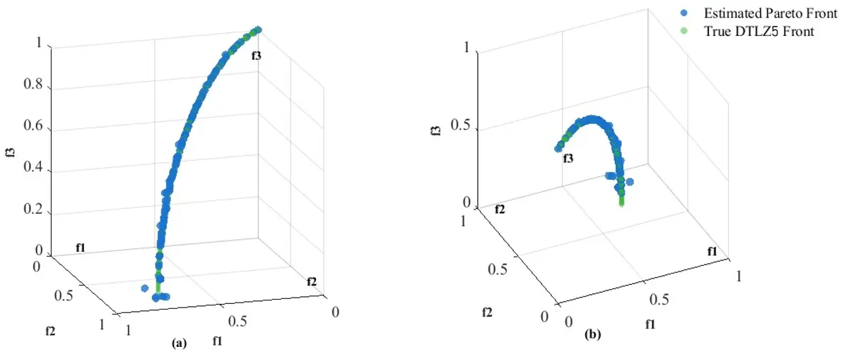
MOPPO’s solution set of DTLZ5 achieves precise coverage of the PF, as shown in Figure 10. Although the nonlinear objective correlations in the DTLZ5 problem pose significant optimization challenges, resulting in a slightly sparse distribution of solutions in the high-f1 and high-f2 regions compared to the true PF, MOPPO demonstrates remarkable adaptability to nonlinear objective interactions, maintaining strong alignment with the true PF.
4.1.2. Convergence Analysis of MOPPO on Benchmark Problems
Figure 11 and Figure 12 present the IGD convergence curves of the three algorithms tested with DTLZ2 and DTLZ5, respectively. MOPPO demonstrates significant advantages in both functions. For test function DTLZ2, MOPPO’s IGD value rapidly declines at early iterations (<50) and stabilizes after approximately 150 iterations. This fast convergence stems from its policy gradient mechanism, which accurately captures intricate objective interactions and effectively resolves high-dimensional trade-offs. In contrast, MOPSO exhibits minor oscillations after 100 iterations due to parameter sensitivity and ultimately converges to a higher IGD value than MOPPO, indicating suboptimal convergence accuracy of the solution set. While MOSFO stagnates at higher IGD values owing to premature convergence, reflecting deviation from the true PF and poor distribution characteristics.
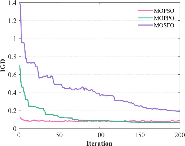
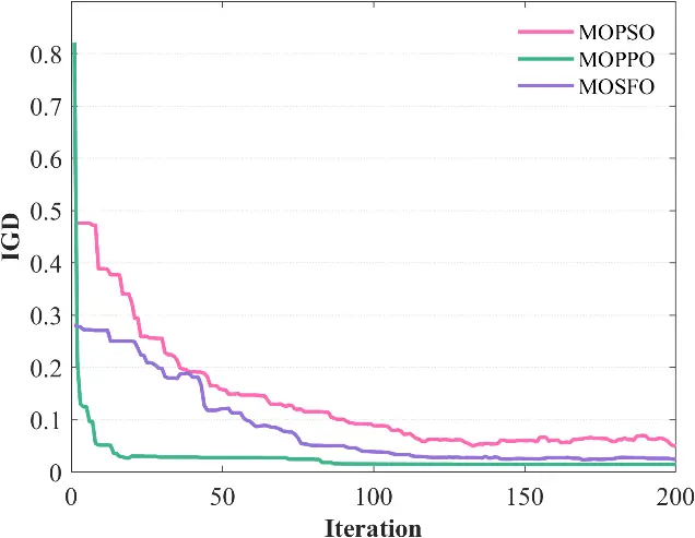
For test function DTLZ5, MOPPO’s IGD curve shows a sharp initial descent. Conversely, MOPSO stalls in later iterations (>150) due to limited local search capability, and MOSFO experiences IGD rebound caused by distribution entropy fluctuations.
The average IGD convergence values of the three algorithms are presented in Table 10. These values were obtained by averaging the final converged IGD results from 50 independent runs on the benchmark problems. Compared to MOPSO and MOSFO, MOPPO achieves 20.8% and 64.0% lower IGD values on DTLZ2, and 41.2% and 75.3% lower on DTLZ5, respectively. These substantial reductions signify that MOPPO’s solution sets exhibit significantly enhanced convergence precision when approximating the true PF.
Table 10. Performance of Algorithms on DTLZ2 and DTLZ3.
|
Algorithm |
IGD of DTLZ2 |
IGD of DTLZ5 |
|---|---|---|
|
MOPPO |
0.0680 |
0.0147 |
|
MOPSO |
0.0859 |
0.0596 |
|
MOSFO |
0.1890 |
0.0250 |
In summary, MOPPO not only maintains a uniform distribution of solutions in the objective space but also rapidly converges to the true PF. This dual advantage makes it particularly suitable for addressing complex multi-objective optimization problems.
4.2. Optimization Results
4.2.1. PF Analysis of MOPPO on IES
To verify the effectiveness and superiority of the proposed MOPPO algorithm in solving the optimal design of the IES, the MOPSO was introduced as a benchmark for comparison. Figure 13 illustrates the Pareto optimal frontiers obtained by MOPPO and MOPSO, explicitly revealing the trade-offs among operational cost, CDERR, and RU. The training of MOPPO on the IES design problem converged after approximately 800 episodes, as evidenced by the stabilization of the average episode reward and the hypervolume of the Pareto front. The PF of MOPPO exhibits the following characteristics: The optimal solution set for daily cost spans from $8730.86 to $15,064.02. Regarding environmental performance, CDERR values cover 48–60%, while the RU range spans 76–97%, with peak values occurring in high-cost regions.
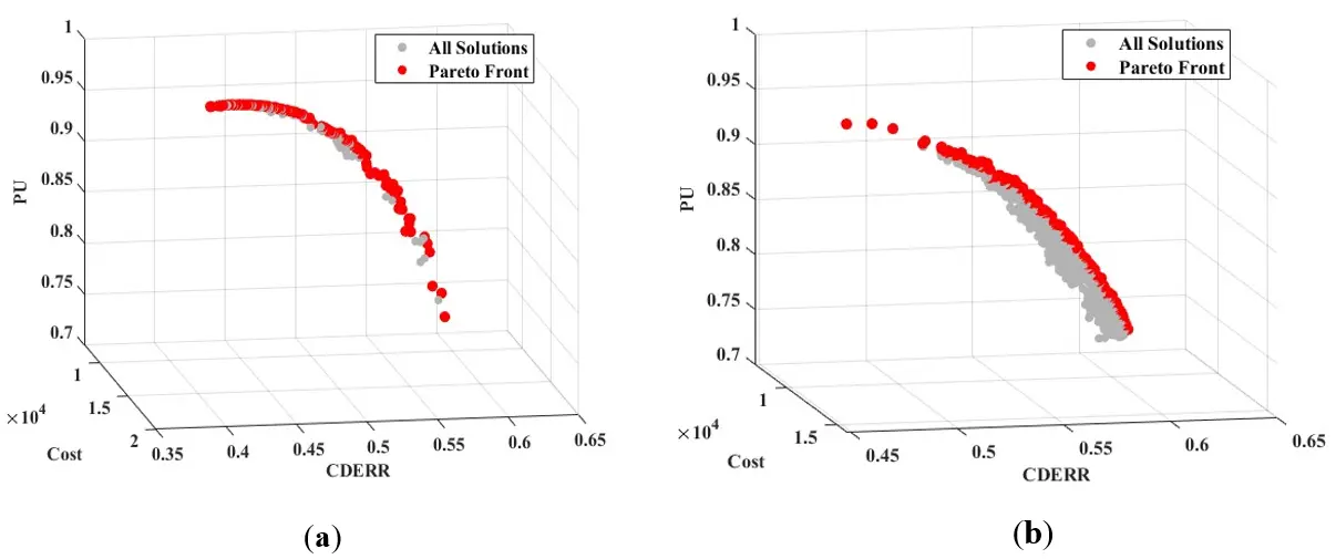
Observation of the Pareto fronts reveals that the solution sets generated by MOPPO and MOPSO exhibit similar distribution trends and coverage ranges in the objective space. This similarity verifies the convergence capability of the MOPPO algorithm, demonstrating that the DRL-based approach can effectively approximate the true Pareto front.
Further analysis of the Pareto front reveals intricate interactions among the three objectives. As RU approaches 1 (indicating near-full renewable utilization), the system requires a high penetration of renewable generation, leading to substantial initial investment costs and consequently an increase in total cost. Concurrently, the CDERR exhibits a slight decline. This inverse relationship originates from an inherent conflict between the optimization objectives: the definition of the RU (Equation (24)) rate inherently discourages electricity sales, while the definition of the CDERR (Equation (21)) necessitates maximizing the total generation from renewables. Consequently, the pursuit of a higher renewable energy utilization rate inhibits the deployment of large-scale renewable capacity to avoid power sales, thereby limiting the achievable carbon emission reduction rate.
The solution distribution shows dense clustering in economically favorable low-cost regions, offering decision-makers flexible options to balance environmental targets within budget constraints. For instance, In scenarios with high carbon trading costs or stringent emission mandates, solutions prioritizing CDERR can be selected. Under energy cost pressures, solutions near the low-cost Pareto region are optimal.
4.2.2. Comprehensive Evaluation of Pareto-Optimal Solutions Using TOPSIS Method
Table 11 presents the comparison of the final optimal design solutions selected by TOPSIS for both algorithms. As indicated in Table 3, although both algorithms provide feasible design schemes, the optimal solution derived from MOPPO outperforms the MOPSO solution in terms of comprehensive performance. Specifically, the MOPPO solution achieves a lower Cost of $16,834.87, representing a 6.52% reduction compared to the $18,009.32 cost of MOPSO. Furthermore, MOPPO demonstrates superior environmental performance, with a CDERR of 59.49%, corresponding to a 9.54% improvement over MOPSO. This superiority can be attributed to the proximal policy optimization mechanism, which enables more stable updates and fine-grained search in the continuous action space of equipment capacity configuration. Consequently, the MOPPO-optimized configuration was selected as the final design scheme for further analysis in the subsequent sections.
Table 11. Optimal capacity configuration.
|
Algorithm |
Cost |
CDERR |
RU |
PV |
WT |
Battery |
Ice Tank |
|---|---|---|---|---|---|---|---|
|
MOPPO |
16,834.87 |
59.49 |
87.02 |
824 |
4 |
9301 |
37,949 |
|
MOPSO |
18,009.32 |
54.31 |
89.96 |
765 |
4 |
9283 |
39,727 |
|
Unit |
USD |
% |
% |
m2 |
- |
kWh |
kWh |
4.3. Analysis of Energy and Economy
In this section, the cooling and electricity balance analysis are presented to show the operational strategies of the IES.
4.3.1. Cooling and Electricity Balance
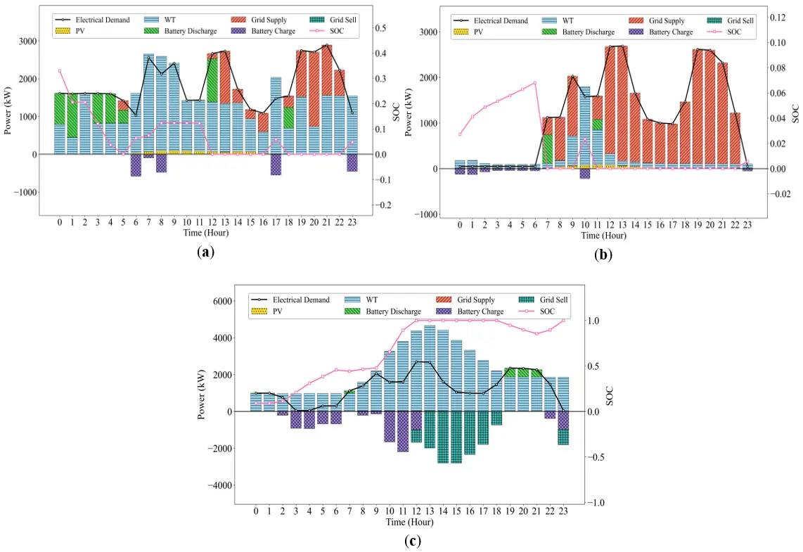
As illustrated in the typical daily electricity balance diagrams for summer, winter, and the transitional seasons in Figure 14, the system shows clear seasonal differences in demand profile, RE usage, and battery storage strategies. During the summer period, the electricity demand between 0:00–5:00 remains relatively higher compared to other seasons due to significantly increased cooling requirements. Wind power generation is insufficient during the 00:00–01:00 and 03:00–05:00 periods. To meet the load gap, the system satisfies the load demand through battery discharge and purchasing power from the grid. After 12:00, except for a local peak at 17:00, renewable energy generation is generally inadequate: photovoltaic power generation is constrained by installed capacity, and wind power output is intermittent, leading to occasional reliance on battery discharge.
In winter, electricity demand is relatively lower, and nighttime load decreases significantly. This is primarily because ice storage cooling mode is not activated in winter, and electricity is mainly used to meet basic cooling load. Although wind power generation is limited between 00:00 and 06:00, it still meets the baseline nighttime load demand, with surplus power used to charge the battery. Daytime wind power exhibits significant fluctuations: except for the peak in wind power generation between 09:00 and 11:00, renewable energy output is noticeably lower during other periods. The battery is depleted by 11:00 and remains at a 0% SOC thereafter. The system primarily relies on grid power to maintain stable operation. By midday, the battery is often fully discharged, and the system relies on grid electricity. Unlike summer, no ice storage is used, and the operational strategy focuses purely on electricity balance.
Transition seasons demonstrate significant advantages in wind power resources. Between 02:00–06:00 and 08:00–12:00, The system prioritizes storing excess electricity in the battery, and by 12:00, the battery’s SOC reaches the upper limit of its rated capacity. Thereafter, all excess wind power is directly transmitted to the grid between 12:00 and 18:00. Throughout this period, the battery remains fully charged at its maximum capacity. This operational mode not only facilitates the utilization of renewable energy but also significantly enhances the system’s economic performance via revenue generated from electricity sales.
The cooling balance across seasons is illustrated in Figure 15. Summer is characterized by high cooling demand and strong solar irradiance, but moderate wind speeds. Due to the temporal mismatch between solar generation and cooling demand, the system relies heavily on ice storage to shift cooling loads. By relying on overnight ice storage, the system meets part of the daytime cooling demand in summer. Specifically, during the nighttime period from 00:00 to 05:00, the system initiates ice-making mode to convert electrical energy into ice for cooling storage. This ice-storage strategy reduces peak power demand during daytime operation. The discharge process of the ice storage from 10:00 to 22:00 shows a gradual decrease in the cooling energy supplied by the ice tank, attributable to the declining melting rate as discussed in Section 2.2.4. It is noteworthy that no ice charging occurs at 17:00, as this period coincides with the peak wind power generation shown in Figure 14. The system prioritizes the use of green electricity to directly drive the chillers for cooling, thereby reducing ice consumption and enhancing the utilization of clean energy.
Because of the residual ice from the previous day, less ice is stored at night on the typical transitional season day than on a summer day. As shown in Figure 15, the duration of ice storage operation in these seasons is only 3 h, significantly shorter than the 6 h in summer. During the daytime (08:00–18:00) of that day, wind and photovoltaic power generation are relatively abundant, enabling renewable electricity to directly power the chillers and meet most of the cooling demand. As a result, the ice storage system remains in standby mode. Between 19:00 and 21:00, when renewable generation declines, the system activates the ice storage to discharge cooling energy, supplementing the chiller output to ensure stable coverage of the cooling load.
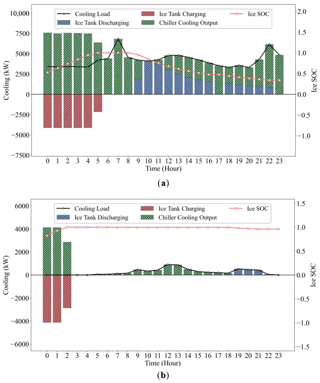
Throughout the summer, the ITES effectively shifts daytime peak electricity demand via coordinated charging and discharging strategies. By prioritizing direct use of surplus green electricity for cooling, the system not only guarantees cooling reliability but also improves economic and environmental performance. In transitional seasons, the operational strategy focuses on maximizing renewable energy consumption, with the ice storage system serving as a supplementary regulation measure. This further enhances the utilization of clean energy and increases the overall economic efficiency of the system.
4.3.2. Seasonal Power Generation Analysis
Figure 16 depicts the energy mix of the system. The results reveal the dominance of RE sources, which maintains a share between 76.7% and 86.8%. It should be noted that the term “Renewable” here refers to direct generation from sources such as wind and PV, while the electricity labeled as “Battery” also originates entirely from renewable sources. Essentially, battery storage captures surplus renewable electricity and discharges it when needed, thereby enabling a temporal shift in the power supply. Renewable contribution reaches its lowest level, at 76.7%, during summer. This decline stems from seasonal attenuation in wind power output and high cooling loads, which elevate grid-supplied electricity to 20.8%. Winter shows negligible cooling demand, and the ice storage system is not activated. The electricity load is dominated by lighting and office equipment. Wind power is generally stronger in winter due to seasonal monsoon effects, contributing to a renewable share of 80.9%.
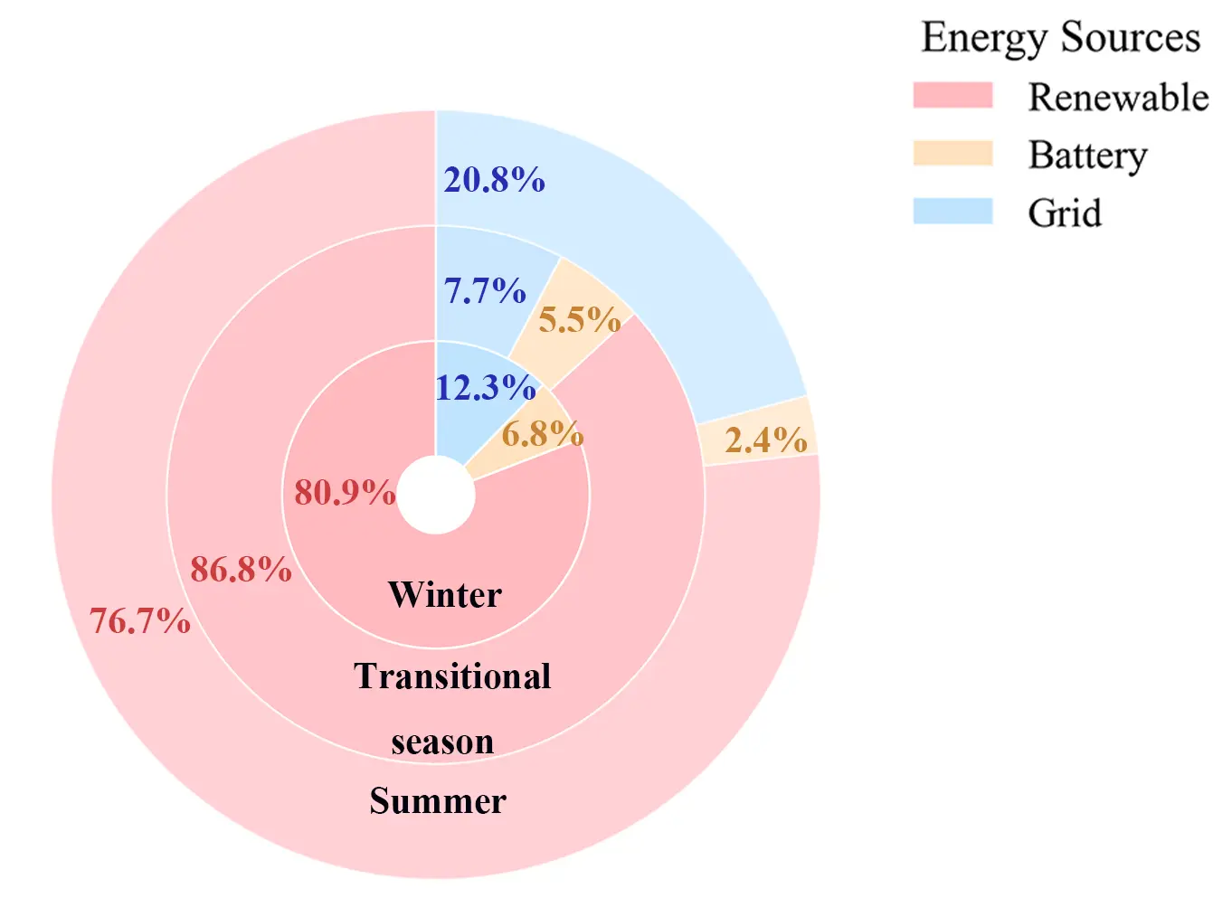
Concurrently, battery output rises to 6.8%, indicating the effectiveness of storage system integration in managing renewable generation. Transition seasons demonstrate optimal performance where mild climates ensure stable wind output and photovoltaic generation, minimizing grid reliance to 7.7%.
Such power generation behavior confirms the climatic resilience of IES. During transition seasons, 92.3% of electricity comes from clean energy sources—renewables together with battery storage. In extreme seasons, grid support becomes essential to maintain power supply reliability. Future optimization can prioritize long-term storage to further reduce dependence on grid supply.
In summary, the seasonal analysis reveals that: (i) summer is the most challenging season due to high cooling demand and moderate wind resources, requiring ice storage and grid backup; (ii) winter relies on battery storage to manage wind variability, with no cooling demand; (iii) transition seasons achieve near-grid-independence through abundant wind resources and low cooling loads. These seasonal differences justify the need for a multi-objective optimization that accounts for year-round performance rather than a single representative day.
4.4. Sensitivity Analysis
4.4.1. Sensitivity Analysis of Design Parameters
In order to further investigate the relationships between the design variables and the objectives, a sensitivity analysis was conducted. The results are shown in Figure 17. The analysis indicates a significant strong correlation between the number of wind turbines and the objective functions. The number of wind turbines is negatively correlated with LCC, demonstrating that increasing the number of turbines significantly reduces system costs. Concurrently, a strong negative correlation exists between the number of wind turbines and the RU. This is primarily attributed to the fact that an increased number of turbines leads to a higher proportion of excess electricity being sold back to the grid, which consequently reduces the system’s renewable energy self-sufficiency. This demonstrates the multifaceted effects of turbine quantity on system performance, necessitating comprehensive trade-offs between cost-effectiveness and dependence on the grid.
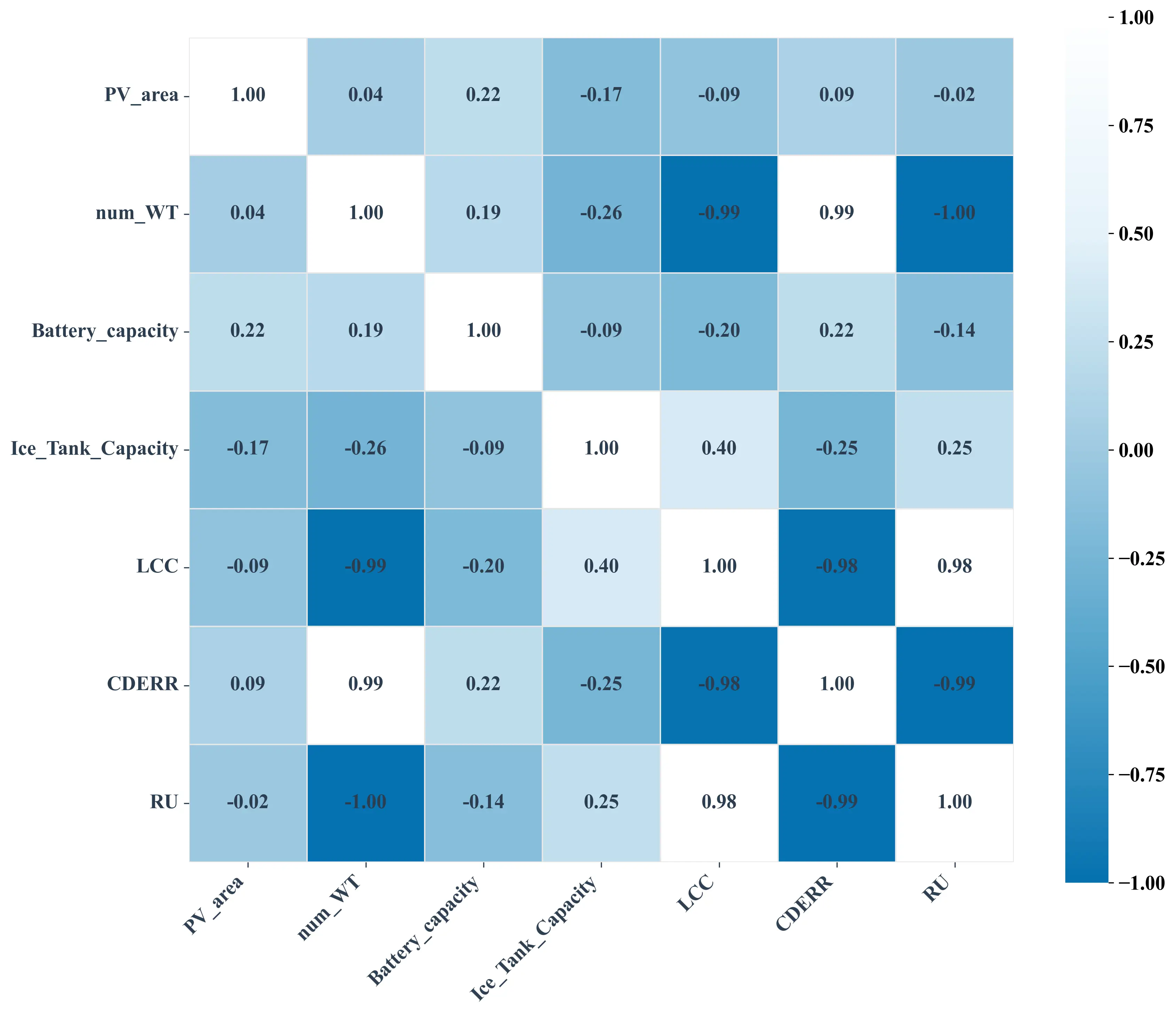
Although PV area exhibits a relatively smaller impact on the objective function, it contributes positively to improving energy efficiency, particularly in enhancing the system’s green benefits. However, the installation of the PV panels is limited by the roof areas. Ice storage capacity shows a positive correlation with LCC, indicating a marginal increase in system lifecycle cost. Nevertheless, it plays an important role in boosting energy utilization efficiency by shifting system load.
Overall, the number of wind turbines exerts the most significant influence during optimization, significantly reducing the LCC of the system while enhancing energy utilization efficiency through improved RE accommodation, and elevating environmental quality via clean energy substitution. Other design variables—PV area, battery capacity, and ice storage capacity—demonstrate varying degrees of impact but remain essential contributors to the optimization process.
Regarding inter-variable relationships, a weak positive correlation exists between the number of wind turbines and battery capacity. This means a potential complementary coordination may emerge during system scaling. For example, batteries could store extra wind power when it’s windy and supply power when the wind slows down. Conversely, a negative correlation between the number of wind turbines and ice storage capacity implies a possible competitive relationship in system design. For instance, with an increase in wind turbines, more renewable energy can be used to power the chillers. The requirement of ice storage is reduced. Furthermore, the positive correlation between ice storage capacity and LCC underscores its substantial contribution to economic burden. In contrast, battery capacity has a weaker impact on cost, indicating that battery energy storage has a comparative advantage over ice storage in terms of economic viability.
4.4.2. Analysis of System Optimization Triggered by Ice Storage Cost
With the continuous technology advancement and large-scale application of ice storage, the unit investment cost is expected to decline steadily. To prospectively evaluate the positive influence of this trend on future integrated energy systems, Figure 18 analyzes the critical role of ice storage unit cost in the optimal configuration of the system.
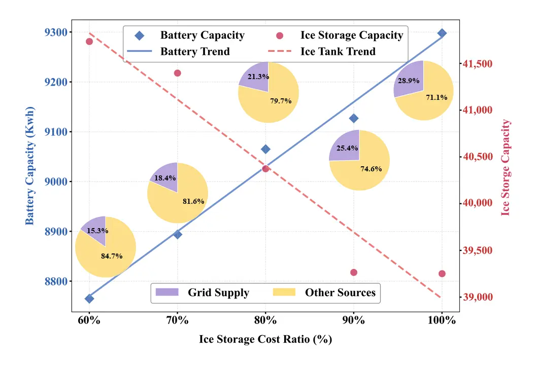
The results indicate that the decrease in the unit cost of the ice storage system not only significantly increases the installed capacity of the ice storage but also triggers an optimization effect on other components of the system. The battery capacity decreases from 9301 kWh to 8765 kWh, which is primarily attributed to the fact that the ice storage system partially substitutes the “peak shaving” function of the battery by shifting cooling loads and reducing daytime electricity peaks, thereby economically reducing the demand for battery capacity. Furthermore, the capacity of renewable energy generation also increases accordingly. This is due to growing electricity demand for ice-making driven by expanded ice storage capacity, as well as the need to generate more power in real time to match daytime loads to compensate for the reduction in battery storage capacity.
In terms of energy, the proportion of grid power supply significantly decreases from 28.9% to 15.3%. This reduction stems from the excellent peak shaving and valley filling capabilities of the ice storage system, synergizing with the increased RE capacity. This combination markedly reduces reliance on the grid during peak periods while promoting the integration of renewable energy.
5. Conclusions
This study proposes an IES incorporating PV, wind turbine, battery storage, ice storage, chillers, and the power grid. An improved MOPPO reinforcement learning algorithm is introduced to address the multi-objective optimization design problem for this system. The algorithm demonstrates suitability for multi-objective reinforcement learning problems. Its effectiveness is validated using standard test functions, and a comprehensive analysis of the system’s energy economics is conducted. Key findings are summarized as follows:
- (1)
-
The superior performance of the improved MOPPO algorithm is validated on standard multi-objective test functions DTLZ2 and DTLZ5. The obtained Pareto fronts closely approximate the true Pareto fronts. When compared with multi-objective metaheuristic algorithms (MOPSO and MOSFO), MOPPO achieves significant reductions in IGD values of 20.8–64.0% on DTLZ2 and 41.2–75.3% on DTLZ5, indicating markedly improved solution accuracy and convergence.
- (2)
-
The improved MOPPO is successfully applied to the optimal design of the IES. The TOPSIS method is used for decision-making, demonstrating that the optimal solution derived from MOPPO outperforms the MOPSO benchmark, achieving a 6.52% reduction in daily operating costs and a 9.54% improvement in the carbon dioxide emission reduction rate.
- (3)
-
Analysis of daily operation across seasons indicates that the designed IES effectively balances the supply and demand. This is achieved through the synergistic operation of electrical and ice storage to enhance system flexibility and efficiency. Battery storage plays a crucial role in storing surplus renewable generation during peak production periods and discharging it to cover supply shortfalls. Simultaneously, the ice storage system significantly contributes to load management by shifting cooling demand from peak to off-peak hours, which effectively reduces daytime electrical loads and enhances the utilization of overnight excess renewable energy. This strategy not only flattens the daily load profile but also significantly increases the self-consumption of renewable energy.
- (4)
-
This study further reveals that a 40% reduction in ice storage unit cost leads to a 6.3% increase in its stalled capacity and a corresponding 5.7% decrease in battery capacity, demonstrating a clear technological substitution effect. Meanwhile, grid dependence decreased significantly from 28.9% to 15.3%, highlighting the system’s improved economic efficiency and renewable self-consumption capability. These findings underscore the importance of cost-effective ice storage in developing future low carbon buildings.
It should be noted that while this study has taken into account factors such as equipment aging and operational maintenance costs, the modeling approach remains relatively simplified. In practical engineering applications, more refined and dynamic modeling analysis tailored to specific scenarios is required. Future work will focus on developing highly detailed models considering equipment performance degradation and energy price uncertainty.
Statement of the Use of Generative AI and AI-Assisted Technologies in the Writing Process
During the preparation of this manuscript, the authors used Generative AI for language polishing and grammar checking. After using this tool, the authors reviewed and edited the content as needed and take full responsibility for the content of the published article.”
Author Contributions
Conceptualization, X.Y. Yang and Y. Li; Methodology, X.Y. Yang; Software, X.Y. Yang; Validation, X.Y. Yang and Y. Li; Formal Analysis, X.Y. Yang; Investigation, X.Y. Yang; Resources, Y. Li; Data Curation, X.Y. Yang; Writing—Original Draft Preparation, X.Y. Yang; Writing—Review & Editing, X.Y. Yang and Y. Li; Visualization, X.Y. Yang; Supervision, Y. Li; Project Administration, Y. Li. All authors have read and agreed to the published version of the manuscript.
Ethics Statement
Not applicable.
Informed Consent Statement
Not applicable.
Data Availability Statement
The data presented in this study are available from the corresponding author upon reasonable request.
Funding
This research received no external funding.
Declaration of Competing Interest
The authors declare that they have no known competing financial interests or personal relationships that could have appeared to influence the work reported in this paper.
Abbreviations
|
Abbreviations |
|
|
IES |
Integrated energy system |
|
DESs |
Distributed energy systems |
|
ACO |
Ant Colony Optimization |
|
PV |
Photovoltaic |
|
SOC |
State of charge |
|
ESSs |
Energy storage systems |
|
PSO |
Particle Swarm Optimization |
|
RE |
Renewable energy |
|
ITES |
Ice thermal energy storage |
|
NSGA |
Non-dominated Sorting Genetic Algorithm |
|
LCC |
Lifecycle cost |
|
ICC |
Initial capital cost |
|
CDERR |
CO2 emission reduction rate |
|
RU |
Renewable energy utilization rate |
|
EMA |
Evolutionary Mating Algorithm |
|
DRL |
Deep Reinforcement Learning |
|
PPO |
Proximal Policy Optimization |
|
NPV |
Net present value |
|
PF |
Pareto front |
|
LSTM |
Long Short-Term Memory |
|
Symbols |
|
|
Qc |
real-time cooling capacity |
|
Qe |
real-time condensing heat output |
|
Gw,c |
cooling water mass flow rate |
|
Gw,e |
chilled water mass flow rate |
|
Pc, Pe |
power consumption of the cooling water pump and the chilled water pump |
|
Pco |
real-time power consumption of the cooling tower |
|
Δt |
time duration for charge or discharge |
|
Pbat |
charge and discharge power |
|
Cbat |
battery capacity |
|
PLRn(t) |
partial load ratio of the n-th ice-making unit at time t |
|
Qn,cap |
rated cooling capacity of the n-th ice-making |
|
Qit |
total capacity of the ice tank |
|
H |
ice melting time |
|
Qm |
maximum ice melting capacity |
|
N |
life span of the system |
|
tr |
tax rate |
|
an |
annual maintenance and operational costs |
|
R |
number of equipment replacements over the system lifecycle |
|
NPV, NWT |
area of installed PV panels and number of wind turbines in the system |
|
NB/NICE |
capacity of the battery storage/ice storage tank |
|
$$\widehat{A_t}$$ |
estimated advantage function at timestep t |
|
$$r_t(\theta)$$ |
probability ratio between the new and old policies |
|
Greeks |
|
|
$$\eta$$ |
The cooling capacity conversion efficiency |
|
$$\beta$$ |
The percentage of melted ice relative to the total ice storage capacity. |
|
$$\epsilon$$ |
clipping range to prevent excessively large policy updates. |
References
- IEA. Buildings—Energy System. Available online: https://www.iea.org/energy-system/buildings (accessed on 1 April 2025).
- Xiong J, Ye Y, Wang Q, Dong X, Lu T, Ma D. A comprehensive review on distributed energy cooperative control and optimization method for energy interconnection system. Electr. Power Syst. Res. 2024, 237, 111007. DOI:10.1016/j.epsr.2024.111007 [Google Scholar]
- Wang M, Yu H, Yang Y, Lin X, Guo H, Li C, et al. Unlocking emerging impacts of carbon tax on integrated energy systems through supply and demand co-optimization. Appl. Energy 2021, 302, 117579. DOI:10.1016/j.apenergy.2021.117579 [Google Scholar]
- Sehar F, Pipattanasomporn M, Rahman S. An energy management model to study energy and peak power savings from PV and storage in demand responsive buildings. Appl. Energy 2016, 173, 406–417. DOI:10.1016/j.apenergy.2016.04.039 [Google Scholar]
- Ullah K, Ali S, Khan TA, Khan I, Jan S, Shah IA, et al. An Optimal Energy Optimization Strategy for Smart Grid Integrated with Renewable Energy Sources and Demand Response Programs. Energies 2020, 13, 5718. DOI:10.3390/en13215718 [Google Scholar]
- Karimi H. A tri-objectives scheduling model for renewable-hydrogen-based microgrid system considering hydrogen storage system and demand-side management. Int. J. Hydrogen Energy 2024, 68, 1412–1422. DOI:10.1016/j.ijhydene.2024.04.330 [Google Scholar]
- Zhu X, Gui P, Zhang X, Han Z, Li Y. Multi-objective optimization of a hybrid energy system integrated with solar-wind-PEMFC and energy storage. J. Energy Storage 2023, 72, 108562. DOI:10.1016/j.est.2023.108562 [Google Scholar]
- Hua LG, Bilal M, Hafeez G, Ali S, Alghamdi B, Alsafran AS, et al. An energy-efficient system with demand response, distributed generation, and storage batteries for energy optimization in smart grids. J. Energy Storage 2025, 117, 115491. DOI:10.1016/j.est.2025.115491 [Google Scholar]
- Sabareesh SU, Aravind KSN, Chowdary KB, Syama S, Devi VSK. LSTM Based 24 hours Ahead Forecasting of Solar PV System for Standalone Household System. Procedia Comput. Sci. 2023, 218, 1304–1313. DOI:10.1016/j.procs.2023.01.109 [Google Scholar]
- Cui X, Zhu J, Jia L, Wang J, Wu Y. A novel heat load prediction model of district heating system based on hybrid whale optimization algorithm (WOA) and CNN-LSTM with attention mechanism. Energy 2024, 312, 133536. DOI:10.1016/j.energy.2024.133536 [Google Scholar]
- Liu B, Xie Y, Wang K, Yu L, Zhou Y, Lv X. Short-Term Multi-Step Wind Direction Prediction Based on OVMD Quadratic Decomposition and LSTM. Sustainability 2023, 15, 11746. DOI:10.3390/su151511746 [Google Scholar]
- Wang L, Mao M, Xie J, Liao Z, Zhang H, Li H. Accurate solar PV power prediction interval method based on frequency-domain decomposition and LSTM model. Energy 2023, 262, 125592. DOI:10.1016/j.energy.2022.125592 [Google Scholar]
- Chen B, Li Z, Li S, Zhao Q, Liu X. A Wind Power Prediction Framework for Distributed Power Grids. Energy 2024, 121, 1291–1307. DOI:10.32604/ee.2024.046374 [Google Scholar]
- Ma Y. Multi-objective optimization model and algorithm implementation of the distributed power generation system for renewable energy in China and Russia. Unconv. Resour. 2025, 7, 100201. DOI:10.1016/j.uncres.2025.100201 [Google Scholar]
- Wang C, Jiao S, Zhang Y, Li Y, Li Y, Zhang Q. A new transfer evolutionary multi-task optimization algorithm for bi-level optimal configuration of distributed generations and energy storage systems considering uncertainties. J. Energy Storage 2025, 113, 115556. DOI:10.1016/j.est.2025.115556 [Google Scholar]
- Yau YH, Rismanchi B. A review on cool thermal storage technologies and operating strategies. Renew. Sustain. Energy Rev. 2012, 16, 787–797. DOI:10.1016/j.rser.2011.09.004 [Google Scholar]
- Curto D, Favuzza S, Franzitta V, Guercio A, Amparo Navarro Navia M, Telaretti E, et al. Grid Stability Improvement Using Synthetic Inertia by Battery Energy Storage Systems in Small Islands. Energy 2022, 254, 124456. DOI:10.1016/j.energy.2022.124456 [Google Scholar]
- Saffari M, de Gracia A, Fernández C, Belusko M, Boer D, Cabeza LF. Optimized demand side management (DSM) of peak electricity demand by coupling low temperature thermal energy storage (TES) and solar PV. Appl. Energy 2018, 211, 604–616. DOI:10.1016/j.apenergy.2017.11.063 [Google Scholar]
- Al-Aali I, Narayanaswamy A, Modi V. Design of chiller system with thermal and battery storage for enhanced integration with on-site PV. J. Build. Eng. 2024, 87, 109072. DOI:10.1016/j.jobe.2024.109072 [Google Scholar]
- Al-Aali I, Modi V. Decarbonizing the electricity sector in Qatar using PV combined with ice thermal and battery storage. Energy Strategy Rev. 2022, 44, 101014. DOI:10.1016/j.esr.2022.101014 [Google Scholar]
- Odufuwa OY, Kusakana K, Numbi BP, Tartibu LK. Optimal energy management of grid-connected PV for HVAC cooling with ice thermal storage system. J. Energy Storage 2024, 77, 109844. DOI:10.1016/j.est.2023.109844 [Google Scholar]
- Luerssen C, Gandhi O, Reindl T, Sekhar C, Cheong D. Life cycle cost analysis (LCCA) of PV-powered cooling systems with thermal energy and battery storage for off-grid applications. Appl. Energy 2020, 273, 115145. DOI:10.1016/j.apenergy.2020.115145 [Google Scholar]
- Arévalo P, Benavides D, Lata‐García J, Jurado F. Techno‐economic evaluation of renewable energy systems combining PV‐WT‐HKT sources: Effects of energy management under Ecuadorian conditions. Int. Trans. Electr. Energy Syst. 2020, 30, e12567. DOI:10.1002/2050-7038.12567 [Google Scholar]
- Qiao Q, Yunusa-Kaltungo A, Edwards RE. Feature selection strategy for machine learning methods in building energy consumption prediction. Energy Rep. 2022, 8, 13621–13654. DOI:10.1016/j.egyr.2022.10.125 [Google Scholar]
- Cha JH, Park J, Yeon SH, Yoon Y, Lee KH. Particle Swarm Optimization for multi-chiller system: Capacity configuration and load distribution. J. Build. Eng. 2024, 98, 110953. DOI:10.1016/j.jobe.2024.110953 [Google Scholar]
- Chen C, Duan S, Cai T, Liu B, Hu G. Optimal Allocation and Economic Analysis of Energy Storage System in Microgrids. IEEE Trans. Power Electron. 2011, 26, 2762–2773. DOI:10.1109/TPEL.2011.2116808 [Google Scholar]
- Benfatma H, Khouidmi H, Bessedik B. Neural network and ACO algorithm-tuned PI controller for MPPT in a hybrid battery-supercapacitor energy storage system within DC micro-grid photovoltaic installations. J. Energy Storage 2025, 120, 116499. DOI:10.1016/j.est.2025.116499 [Google Scholar]
- Zakaria NF, Sulaiman MH, Mustaffa Z. Feature optimization with metaheuristics for Artificial Neural Network-based chiller power prediction. J. Build. Eng. 2025, 105, 112561. DOI:10.1016/j.jobe.2025.112561 [Google Scholar]
- Chen B, Zeng W, Nie H, Deng Z, Yang W, Yan B. Optimal load distribution control for airport terminal chiller units based on deep reinforcement learning. J. Build. Eng. 2024, 97, 110787. DOI:10.1016/j.jobe.2024.110787 [Google Scholar]
- Biemann M, Scheller F, Liu X, Huang L. Experimental evaluation of model-free reinforcement learning algorithms for continuous HVAC control. Appl. Energy 2021, 298, 117164. DOI:10.1016/j.apenergy.2021.117164 [Google Scholar]
- Mnih V, Kavukcuoglu K, Silver D, Rusu AA, Veness J, Bellemare MG, et al. Human-level control through deep reinforcement learning. Nature 2015, 518, 529–533. DOI:10.1038/nature14236 [Google Scholar]
- Peng H, Yuan D, Jiang K, Xu W. PPO-based fluctuation-consumption co-optimized energy management for wind-disturbed fuel cell hybrid electric flying car. J. Power Sources 2025, 647, 237349. DOI:10.1016/j.jpowsour.2025.237349 [Google Scholar]
- Ning D, Chen X, Chen J, Meng T, Xu B, Zhang H. PPO-MixClip: An energy scheduling algorithm for low-carbon parks. Energy Rep. 2024, 12, 4195–4207. DOI:10.1016/j.egyr.2024.09.042 [Google Scholar]
- Singh A, Panigrahi BK. A HEN-PPO strategy for home energy management system with reduce EV anxieties. e-Prime Adv. Electr. Eng. Electron. Energy 2024, 10, 100871. DOI:10.1016/j.prime.2024.100871 [Google Scholar]
- Bai L, Tan Z. Optimizing energy efficiency, thermal comfort, and indoor air quality in HVAC systems using a robust DRL algorithm. J. Build. Eng. 2024, 98, 111493. DOI:10.1016/j.jobe.2024.111493 [Google Scholar]
- Ge Y, Xie J, Chang J, Feng S. A multi-objective deep reinforcement learning method for intelligent scheduling of wind-solar-hydro-battery complementary generation systems. Int. J. Electr. Power Energy Syst. 2025, 167, 110635. DOI:10.1016/j.ijepes.2025.110635 [Google Scholar]
- Long Short-Term Memory—An Overview|ScienceDirect Topics. Available online: https://www.sciencedirect.com/topics/engineering/long-short-term-memory (accessed on 17 May 2025).
- Diniz APM, Ciarelli PM, Salles EOT, Coco KF. Use of deep neural networks for clogging detection in the Submerged Entry Nozzle of the continuous casting. Expert Syst. Appl. 2024, 238, 121963. DOI:10.1016/j.eswa.2023.121963 [Google Scholar]
- Tang C, Li N, Bao L. Predictive Control Modeling of Regional Cooling Systems Incorporating Ice Storage Technology. Buildings 2024, 14, 2488. DOI:10.3390/buildings14082488 [Google Scholar]
- Kang J, Wang J, Liu C, Ye S, Yang M. Coordinated optimization of configuration and operation of a photovoltaic integrated building cooling system with electricity and ice storages under source-load uncertainties. Energy Build. 2024, 320, 114600. DOI:10.1016/j.enbuild.2024.114600 [Google Scholar]
- Chen Q, Wei W, Li N. Techno-economic control strategy optimization for water-source heat pump coupled with ice storage district cooling system. Int. J. Refrig. 2022, 138, 148–158. DOI:10.1016/j.ijrefrig.2022.03.010 [Google Scholar]
- Ren X, Han Z, Ma J, Xue K, Chong D, Wang J, et al. Life-cycle-based multi-objective optimal design and analysis of distributed multi-energy systems for data centers. Energy 2024, 288, 129679. DOI:10.1016/j.energy.2023.129679 [Google Scholar]
- Schulman J, Wolski F, Dhariwal P, Radford A, Klimov O. Proximal Policy Optimization Algorithms. arXiv 2017, arXiv:1707.06347. DOI:10.48550/arXiv.1707.06347 [Google Scholar]
- Dingcheng H, Metwally ASM, Ali S, Sillanpaa M, Yassen W, Sobhani B. Sustainable and environmentally-friendly multi-generation system of power, cooling, and hydrogen; Multi-objective optimization using particle swarm algorithm. Appl. Therm. Eng. 2023, 225, 120093. DOI:10.1016/j.applthermaleng.2023.120093 [Google Scholar]
- He W, Xu Q, Guo R, Liu S, Wang Y, Guo H, et al. Optimization analysis of different distributed energy configurations for data centers. Sustain. Mater. Technol. 2024, 41, e01005. DOI:10.1016/j.susmat.2024.e01005 [Google Scholar]
- DKA Solar Centre. Available online: https://dkasolarcentre.com.au/ (accessed on 3 June 2025).
- Chen Y, Xu J. Solar and wind power data from the Chinese State Grid Renewable Energy Generation Forecasting Competition. Sci. Data 2022, 9, 577. Available online: https://www.nature.com/articles/s41597-022-01696-6 (accessed on 3 June 2025).
- Yan R, Zhao T, Rezgui Y, Kubicki S, Li Y. Transferability and robustness of a data-driven model built on a large number of buildings. J. Build. Eng. 2023, 80, 108127. DOI:10.1016/j.jobe.2023.108127 [Google Scholar]
- Yan R, Chen Z, Zhang X, Zhao T, Rezgui Y, Li Y. A novel model ensemble method based on self-adaptive weight for building energy transfer learning. J. Build. Eng. 2025, 109, 113024. DOI:10.1016/j.jobe.2025.113024 [Google Scholar]