
An Effective and Computationally Efficient Similarity-Based Method for Fault Region Identification in Electrical Distribution Systems

An Effective and Computationally Efficient Similarity-Based Method for Fault Region Identification in Electrical Distribution Systems
Joaquim Siqueira de Lima
Ricardo Caneloi dos Santos
*
 Eduardo Werley Silva dos Ângelos
Edmárcio Antônio Belati
Guilherme Torres de Alencar
Alisson Mesquita da Silva
Eduardo Werley Silva dos Ângelos
Edmárcio Antônio Belati
Guilherme Torres de Alencar
Alisson Mesquita da Silva
Received: 02 June 2026 Revised: 03 July 2026 Accepted: 14 August 2026 Published: 28 August 2026

© 2026 The authors. This is an open access article under the Creative Commons Attribution 4.0 International License (https://creativecommons.org/licenses/by/4.0/).
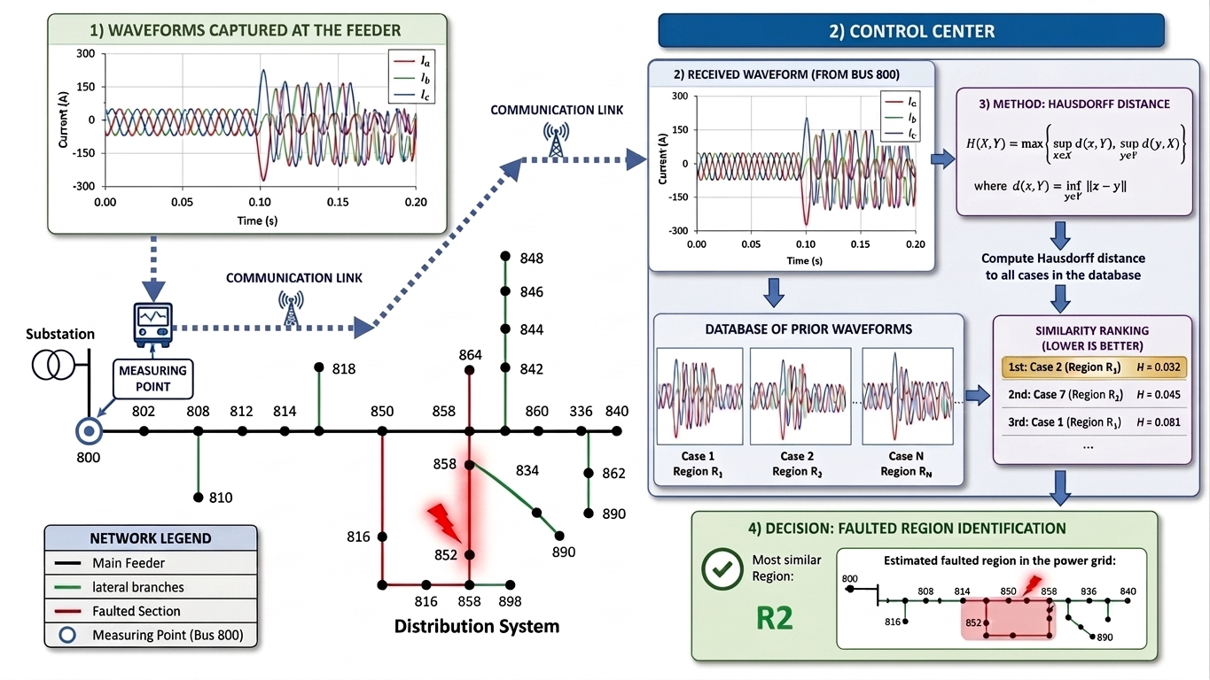
Graphical Abstract
1. Introduction
As power distribution systems continue to grow in size and complexity, distribution line outages increasingly affect customers, requiring more time and resources to locate and repair potential faults. As a result, it is important for utilities to identify fault locations as quickly as possible to improve system availability and minimize economic losses.
The effectiveness of fault location algorithms depends on the operating conditions and the availability of information related to the power grid. With advances in computational power, Artificial Intelligence (AI)-based methods have emerged as an attractive alternative to perform this function, primarily because they do not require detailed distribution system parameters. In this context, Refs. [1,2,3,4,5] developed methodologies based on Artificial Neural Networks (ANNs), however, always requiring a previous training step with a large amount of data.
Another important aspect to consider in distribution systems is the growing penetration of distributed generation (DG). By considering this issue, Refs. [6,7,8,9,10] employed different techniques such as ANNs, Support Vector Machine (SVM), and Wavelet Transform (WT) for locating faults in distribution networks. It is important to note that the accuracy of such methods is directly influenced by three main factors: unbalanced conditions, fault resistance (FR), and the existence of multiple generation sources on the grid. Depending on the levels of these three factors, the methods discussed may be inefficient.
The problem of fault detection and location can also be addressed using concepts of similarity between electrical signals. In [11,12], the authors proposed a fault location method based on similarity analysis. The Fréchet distance is applied to estimate the fault direction by comparing current waveforms, thereby identifying the most probable location of the faulty section. In [13,14], the authors employed the Euclidean distance as a similarity measure to perform the FD function, demonstrating that this approach is a simple and robust alternative that does not require complex formulations or significant computational effort.
More elaborate metrics for assessing similarity, such as the Hausdorff distance (HD), may have greater potential for applications in electrical distribution systems [15]. In [16] was demonstrated that, by analyzing the similarity of transient zero-sequence current waveforms, the fault point can be determined by comparing the modified HD of the transient zero-sequence current in each section of the faulted feeder. In [17] was proposed a new section location method for multistage feeders in distribution grids, based on the use of Spearman’s correlation coefficient. In this study, by analyzing the characteristics of the zero-sequence component of the fault current at buses upstream and downstream of the fault point, and employing the HD, the faulted section can be effectively located. With respect to distribution system applications, Ref. [18] employed the HD to develop a novel load prediction method. The method was tested in a real system, yielding promising results and demonstrating the potential of HD-based methods for applications in real-world problems related to electrical systems. Although the methods discussed demonstrate potential applications, some of them assume the availability of a Wide Area Monitoring System (WAMS), which requires Phasor Measurement Units (PMUs) and data concentrators. This fact is not yet a reality in many power grids, making fault location methods more complex and expensive.
It is worth noting that, as highlighted in the literature, the HD is particularly suitable for fault waveform comparison because it evaluates waveform similarity without requiring time synchronization or point-to-point data correspondence. Furthermore, it can be implemented to be inherently robust to noise, data outliers, and phase shifts, which are common disturbances that affect fault transient [19]. Therefore, Ref. [20] proposed a faulty feeder selection method based on HD to address the low accuracy of faulty feeder selection caused by the complex structure of AC distribution systems. Similarly, Ref. [21] presented an adaptive current differential protection method based on HD, employing waveform similarity comparison to improve the accuracy of protection systems applied to power grids with distributed generation. In [22] was developed a robust faulted line-section location method based on HD algorithm for detecting single-phase-to-ground faults in distribution networks.
Considering the changes experienced by modern distribution power grids, the promising results obtained with similarity-based methods in power system applications, and the need for new solutions to improve utility indices and power system availability, this work proposes a new faulted region identification method based on HD.
The proposed method is simple, fast, and robust, relying only on basic concepts, local current signals, and available resources, which makes it readily applicable to practical situations. The main advantages and contributions of the proposed method are as follows:
-
-
Only local fault current waveforms are required, without the need for communication links;
-
-
The method can be improved over time by updating the database with additional real cases or simulation data;
-
-
Accurate performance was achieved under different fault characteristics and operating conditions;
-
-
No additional hardware resources are required, as the method is based on a waveform pattern-matching approach that can be executed on a conventional personal computer;
-
-
The method is simple, robust, and accurate, representing an excellent alternative to conventional procedures used by utilities.
This paper is organized as follows. Section 2 presents the key concepts related to the adopted technique and the proposed similarity-based method. Section 3 discusses the steps involved in developing and testing the faulted region identification method using a simple distribution system with distributed generation. In Section 4, the proposed HD-based method is validated using the IEEE 34-bus test system. Finally, the conclusions are presented in Section 5.
2. Hausdorff Distance in Fault Analysis
Establishing a certain level of similarity is fundamental to the high performance of various automated systems, whether comparing characters, linguistic expressions, or images. The task of measuring the degree of proximity between two sets remains a persistent challenge for developers, particularly when considering factors such as efficiency and computational cost. The fault region identification problem can also be framed in this context, where decisions can be made based on the degree of similarity between sets of samples from a faulty electrical system, such as voltage or current measurements. As will be shown, by comparing current waveforms acquired from the field with those previously stored in a database, HD enables the implementation of a waveform pattern-matching mechanism, allowing the identification of faulted regions in distribution systems.
2.1. Hausdorff Distance and Evaluation of Signals Similarity
The Hausdorff distance (HD) owes its definition to the efforts of Felix Hausdorff and is widely used in computer vision [15]. Originally, HD is defined as shown in Equations (1) to (3):
where $$A=\left\{{a}_{1}, {a}_{2}, \cdots , {a}_{m}\right\}$$ and $$B=\left\{{b}_{1}, {b}_{2}, \cdots , {b}_{n}\right\}$$ are two finite sets, and ∥⋅∥ is a measure of distance between two points, such as the Euclidean distance or the Manhattan distance.
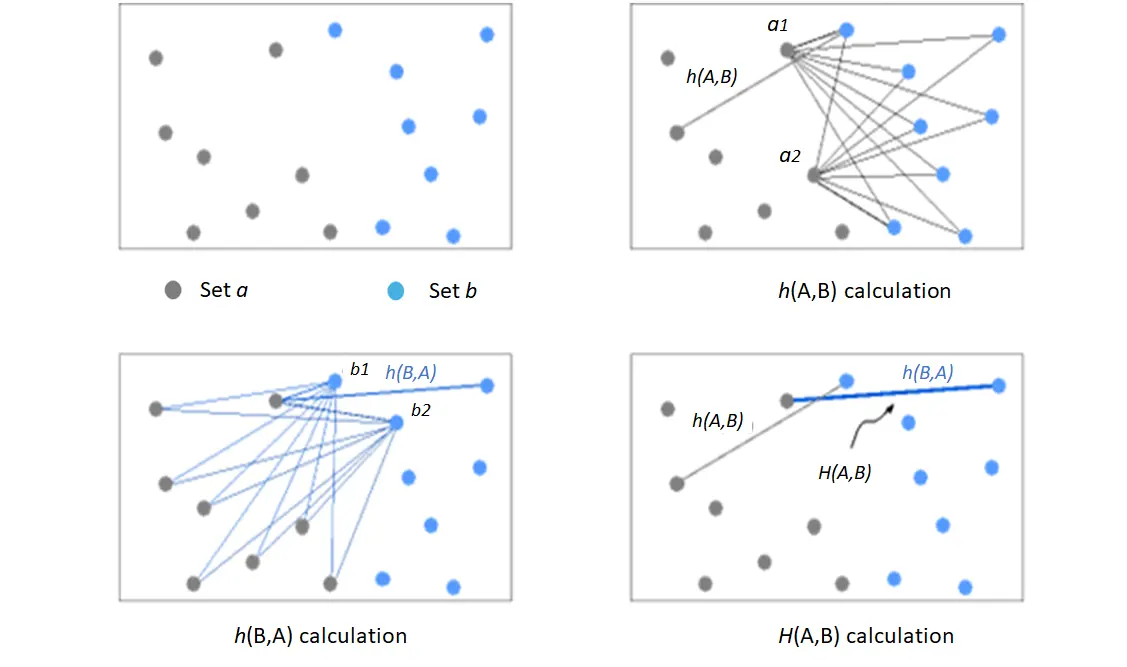
The function $$h\left(A,B\right)$$ is called the Hausdorff directed distance from $$A$$ to $$B$$ for identifying the farthest point $${a}_{i}\in A$$ from its nearest neighbors in $$B$$. The expression $$h\left(B,A\right)$$ is defined similarly, but considers the distance from $$B$$ to $$A$$ instead. In general, $$h\left(A,B\right)\ne h\left(B,A\right)$$. Finally, the Hausdorff Distance $$H\left(A,B\right)$$ will be given by the maximum value between $$h\left(A,B\right)$$ and $$h\left(B,A\right)$$, representing the degree of compatibility between the two sets. A graphical representation of the HD for two-dimensional sets is shown in Figure 1.
The HD can be used to establish the similarity between any two discrete signals or sets of samples. In this case, a measured waveform is represented by a set of samples, and each sample from that waveform is compared to another set of samples relative to a reference waveform. This process is illustrated in Figure 2.
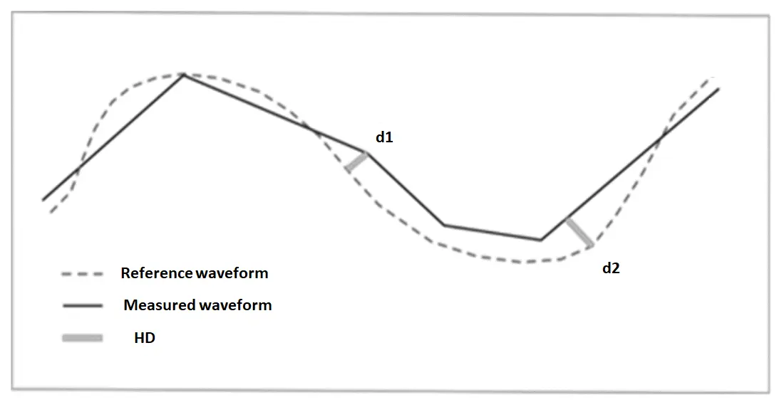
In the case illustrated in Figure 2, after sampling a measured waveform, the comparison between these samples and the previously stored samples that represent the reference waveform must be performed. Thus, the HD is calculated as follows:
-
Calculate the shortest distance from each sample of the measured waveform to all samples of the reference waveform;
-
Store the largest value of all the smallest calculated distances ($${d}_{1}$$);
-
Calculate the shortest distance from each sample of the reference waveform to all samples of the measured waveform;
-
Store the largest value of all the smallest calculated distances ($${d}_{2}$$);
-
Define the HD as the highest value found in steps 2 and 4.
2.2. Methodology for Fault Location Using Hausdorff Distance
This paper proposes a method that identifies the faulted region in primary distribution feeders, based on the comparison between fault signals measured in the field and reference signals stored in a database. In this context, the proposed HD-based method will be applied to assess the similarity between fault current signals measured at the substation and stored signals obtained from simulations or historical events. It is assumed that the fault has already been detected and that the fault current waveform is recorded and available in the digital relay responsible for the feeder. Thus, the oscillography can be recovered (automatically or on demand) and processed at a local or regional operational center.
To exemplify how the method works, it is assumed that for a given fault event, the current $${I}_{a}^{F}$$ was measured (and stored) in the substation digital relay using a sampling rate $${t}_{A}$$. Additionally, it is assumed that a set with $${n}_{f}$$ reference current signals ($${I}_{a}^{{R}_{1}}, {I}_{a}^{{R}_{2}}, \dots , {I}_{a}^{{R}_{{n}_{f}}}$$), representative of different fault events, are available in the database located at the operational center. For each event included in the database, there is a unique fault location associated with it. At this point, it is important to mention that phase a was used to develop this explanation, but a similar procedure can be extended to phases b and c. Once again, it is emphasized that the fault has already been detected, as this method is intended to support operators in the decision-making process, operating in offline mode. Regarding this proposal, the fault location problem in distribution feeders can be formulated as follows:
where $$HD\left({I}_{a}^{F},{I}_{a}^{{R}_{i}}\right)$$ is the Hausdorff distance between the measured fault current $${I}_{a}^{F}$$ and the one recorded in the database $${I}_{a}^{{R}_{i}}$$. In this way, the most likely fault location should correspond to the lowest HD.
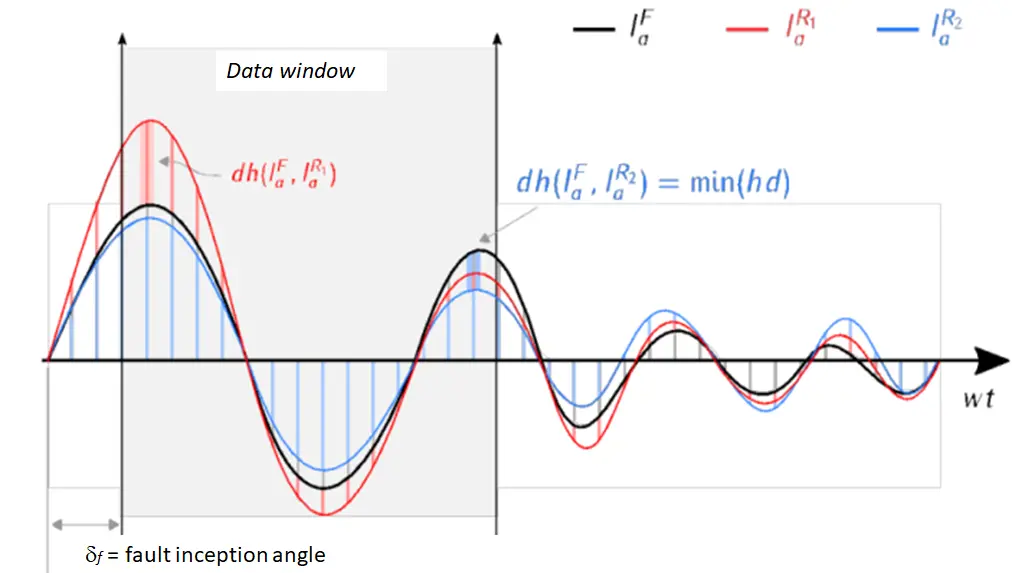
This process is illustrated in Figure 3, where the initial and final instants define the data window length. In this context, $${\delta }_{f}$$ denotes the fault inception angle (FIA). After assessing the similarity between the measured fault current $${I}_{a}^{F}$$ and all historical records of fault events, the lowest HD value will indicate the most likely fault location.
As can be seen, the idea behind this proposal is simple, as the measured current waveform from the field is compared one-to-one with all other waveforms stored in a database. With respect to the example shown in Figure 3, where the database has only two historical events (red and blue fault current waveforms), the blue waveform is the found solution, as it has the shortest HD to the test current waveform. Therefore, the location associated with the blue waveform will be presented as the possible fault location, providing support to the system operator during the decision-making process, when specifying the right place to send the maintenance team. In real-world scenarios, the database may include thousands of historical events obtained from simulations and/or oscillography records from IEDs stored over time.
3. Electrical System and Analysis
The HD-based method presented was developed and validated by considering two different distribution systems, i.e., the IEEE 5-bus test system and the IEEE 34-bus test system. The first one is a distribution network with three generation sources and loads distributed throughout the system. This one, smaller than the second one, was adopted for developing and testing the proposed solution, while the second one, larger and more complex, was used to validate the proposed method, showing its comprehensiveness and accuracy.
3.1. Method’s Evaluation Using the IEEE 5-Bus Test System
The first test system is shown in Figure 4. The diagram represents a 9 MW wind farm equipped with asynchronous generators that export power to a 120 kV grid via a 25 kV distribution feeder. The 120 kV main power supply is modeled as a voltage source with a short-circuit capacity of 1200 MVA. A smart meter (IED) is assumed to be installed upstream of bus B120, where the fault signals are measured and subsequently compared with the corresponding signals stored in the database (DB).
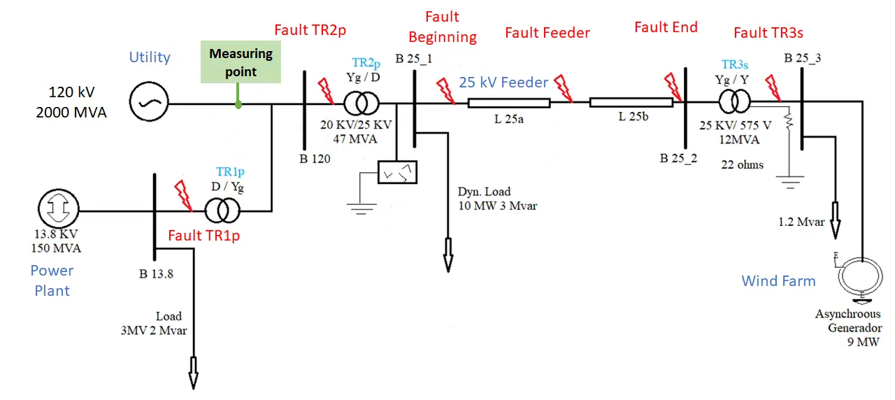
To build the database of fault current waveforms, single-phase faults were simulated at six locations, as shown in Figure 4. These locations were labeled as follows: TR1p (primary side of transformer TR1), TR2p (primary side of transformer TR2), Bus (beginning of the feeder), Feeder (along the feeder), End (end of the feeder), and TR3s (secondary side of transformer TR3). Several fault events were generated assuming different fault resistances, fault locations, and fault inception angles. This work focuses exclusively on single-phase faults, as they constitute the vast majority of faults in distribution systems, accounting for approximately 85% of all fault events. Therefore, they represent the main concern for electric utilities [22].
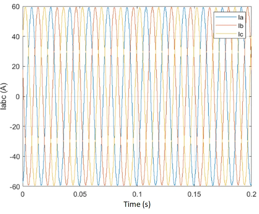
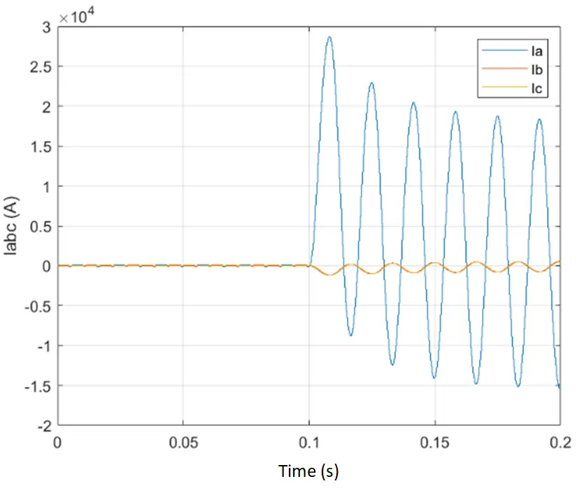
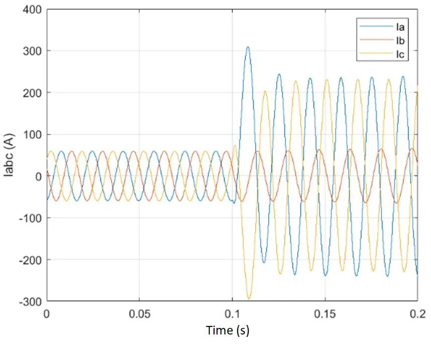
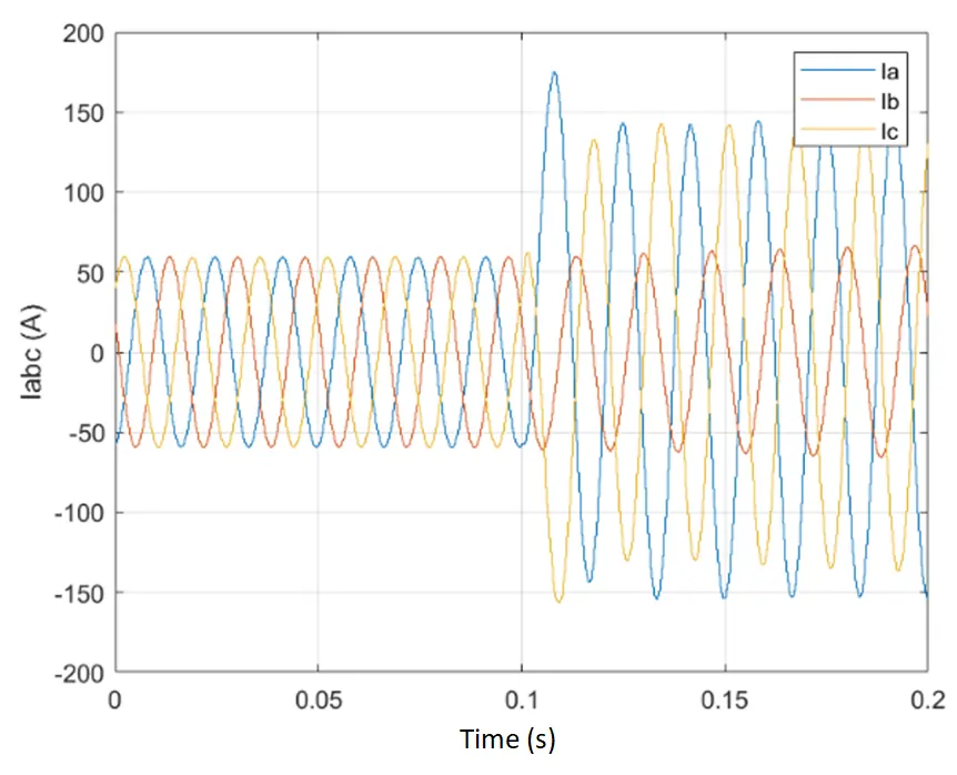
As demonstrated in Figure 5, each fault location presents a distinct fault current signal, which can be considered a fault signature.
 (a) |
 (b) |
 (c) |
 (d) |
Figure 5. Different faults cases in the IEEE 5-bus test system, where: (a) fault at TR1p; (b) fault at TR2p; (c) fault at the midpoint of the feeder (12.5 km); and (d) fault at the far end of the feeder (25 km).
The DB was generated considering the following parameters:
-
-
Fault resistance: $$FR$$ {0; 5; 10; 15; 20} [Ω];
-
-
Fault inception angle: $$FIA$$ {0; 45; 90; 135} [°];
-
-
Fault location on the 25 kV feeder: {2.5; 7.5; 12.5; 17.5; 22.5} [km].
Considering all possible combinations of the mentioned parameters, a DB containing 100 cases was generated. Firstly, when developing the method, a sensitivity analysis was performed with different values of sampling rate ($${t}_{A}$$) and number of windows ($${n}_{j}$$). Subsequently, when testing the method, scenarios with variation of fault resistances and fault inception angles were considered.
3.1.1. Sensitivity Analysis with Respect to Sample Rate and Number of Windows
The first test aims to analyze the sensitivity of the proposed method, considering different sampling rates ($${t}_{A}$$) and number of windows ($${n}_{j}$$). It is worth noting that all these tests considered only single-phase faults, which are more frequent in distribution systems. The main goal of this section is to define the values of $${t}_{A}$$ and $${n}_{j}$$ that make the method more accurate and feasible for practical applications. The following values for $${t}_{A}$$ (in samples by cycle) and $${n}_{j} \left(\mathrm{i}\mathrm{n}\mathrm{ }\mathrm{c}\mathrm{y}\mathrm{c}\mathrm{l}\mathrm{e}\right)$$ were considered, totaling nine combinations:
| $${t}_{A}=64,\mathrm{ }{\mathrm{ }n}_{j}=1/2$$; $${\mathrm{ }t}_{A}=64,\mathrm{ }{\mathrm{ }n}_{j}=1$$; $${t}_{A}=64,\mathrm{ }{\mathrm{ }n}_{j}=2$$; $${t}_{A}=128,\mathrm{ }{\mathrm{ }n}_{j}=1/2$$; $${t}_{A}=128,\mathrm{ }{n}_{j}=1$$; $${t}_{A}=128,\mathrm{ }{n}_{j}=2;\mathrm{ }{t}_{A}=256,\mathrm{ }{n}_{j}=1$$; $${t}_{A}=256,\mathrm{ }{\mathrm{ }n}_{j}=1$$ ; $${t}_{A}=256,\mathrm{ }{\mathrm{ }n}_{j}=2$$. |
The results are presented in Table 1 and Table 2. For each fault case tested, the HD was calculated, and the response associated with the nearest stored event was given. A green symbol “✓” is used in cases where the event with the lowest HD matched the exact fault location. Cases that did not match are indicated by the red symbol “✓”. Initially, only test faults pre-existing in the DB were considered (Table 1), i.e., those with both fault resistance and fault inception angle equal to zero. Subsequently, new cases were tested under conditions not previously included in the DB (Table 2).
Table 1. Sensitivity test for $$FR=0 \, \mathrm{\Omega }$$ and $$FIA=0°$$.
|
Fault Location |
tA = 64 |
tA = 128 |
tA = 256 |
||||||
|---|---|---|---|---|---|---|---|---|---|
|
1/2 |
1 |
2 |
1/2 |
1 |
2 |
1/2 |
1 |
2 |
|
|
TR1p |
✓ |
✓ |
✓ |
✓ |
✓ |
✓ |
✓ |
✓ |
✓ |
|
TR2p |
✓ |
✓ |
✓ |
✓ |
✓ |
✓ |
✓ |
✓ |
✓ |
|
TR3s |
✓ |
✓ |
✓ |
✓ |
✓ |
✓ |
✓ |
✓ |
✓ |
|
Beginning |
✓ |
✓ |
✓ |
✓ |
✓ |
✓ |
✓ |
✓ |
✓ |
|
Feed. 2.5 km |
✓ |
✓ |
✓ |
✓ |
✓ |
✓ |
✓ |
✓ |
✓ |
|
Feed. 7.5 km |
✓ |
✓ |
✓ |
✓ |
✓ |
✓ |
✓ |
✓ |
✓ |
|
Feed. 12.5 km |
✓ |
✓ |
✓ |
✓ |
✓ |
✓ |
✓ |
✓ |
✓ |
|
Feed. 17.5 km |
✓ |
✓ |
✓ |
✓ |
✓ |
✓ |
✓ |
✓ |
✓ |
|
Feed. 22.5 km |
✓ |
✓ |
✓ |
✓ |
✓ |
✓ |
✓ |
✓ |
✓ |
|
End |
✓ |
✓ |
✓ |
✓ |
✓ |
✓ |
✓ |
✓ |
✓ |
Table 2. Sensitivity test for $$FR=12 \, \mathrm{ }\mathrm{\Omega }$$ and $$FIA=70°$$.
|
Fault Location |
tA = 64 |
tA = 128 |
tA = 256 |
||||||
|---|---|---|---|---|---|---|---|---|---|
|
1/2 |
1 |
2 |
1/2 |
1 |
2 |
1/2 |
1 |
2 |
|
|
TR1p |
✓ |
✓ |
✓ |
✓ |
✓ |
✓ |
✓ |
✓ |
✓ |
|
TR2p |
✓ |
✓ |
✓ |
✓ |
✓ |
✓ |
✓ |
✓ |
✓ |
|
TR3s |
✓ |
✓ |
✓ |
✓ |
✓ |
✓ |
✓ |
✓ |
✓ |
|
Beginning |
✓ |
✓ |
✓ |
✓ |
✓ |
✓ |
✓ |
✓ |
✓ |
|
Feed. 2.5 km |
✓ |
✓ |
✓ |
✓ |
✓ |
✓ |
✓ |
✓ |
✓ |
|
Feed. 7.5 km |
✓ |
✓ |
✓ |
✓ |
✓ |
✓ |
✓ |
✓ |
✓ |
|
Feed. 12.5 km |
✓ |
✓ |
✓ |
✓ |
✓ |
✓ |
✓ |
✓ |
✓ |
|
Feed. 17.5 km |
✓ |
✓ |
✓ |
✓ |
✓ |
✓ |
✓ |
✓ |
✓ |
|
Feed. 22.5 km |
✓ |
✓ |
✓ |
✓ |
✓ |
✓ |
✓ |
✓ |
✓ |
|
End |
✓ |
✓ |
✓ |
✓ |
✓ |
✓ |
✓ |
✓ |
✓ |
As can be seen from Table 1 and Table 2, when the method is tested by using pre-existing events, the results are always correct, regardless tA and nj. On the other hand, when using new events, the sampling rate of 64 samples per cycle must be disregarded, regardless of the number of windows employed. For the other cases, a hit rate of 90% was achieved, regardless of tA and nj. As will be discussed, this performance can be further improved by including additional cases in the DB.
3.1.2. Analysis of Different Fault Resistances, Locations, and Inception Angles
This section presents the results considering fault cases with different resistances, locations, and inception angles. The tested faults were located at 5, 10, 15, and 20 km, with fault resistances and inception angles as listed in Table 3. These test cases do not correspond to any fault configurations stored in the historical database. The test faults were evaluated using the two best sampling rates identified in the previous section (tA = 128 and 256), with nj = 1.
The performance in locating faults is evaluated considering the error of the estimated distance in relation to the actual distance of the fault, according to Equation (5):
where $${distance}_{real}$$ is the real fault distance from the substation and $${distance}_{HD}$$ the distance computed by using HD, while $${L}_{s}$$ is the section length under analysis.
It is worth noting that Equation (5) represents the standard approach for measuring the error in fault distance estimation for distribution feeders and transmission lines. The factor (L) expresses the estimation error as a percentage, making it possible to compare fault location methods across different power systems [23].
Table 3 presents the fault distance estimation errors, expressed as a percentage of the distance to the fault location. Larger errors were observed for faults located at the remote end of the feeder. However, new cases can be added to the DB to improve the method’s performance under these conditions, emphasizing that updating the DB is a quick and straightforward process.
Table 3. Percentage errors for different fault distances and fault parameters ($${t}_{A}=128$$, $${n}_{j}=1$$).
|
Fault (km) |
2.5 Ω |
7.5 Ω |
12.5 Ω |
||||||
|---|---|---|---|---|---|---|---|---|---|
|
20° |
60° |
100° |
20° |
60° |
100° |
20° |
60° |
100° |
|
|
0 |
|||||||||
|
5 |
|||||||||
|
10 |
|||||||||
|
15 |
|||||||||
|
20 |
|||||||||
|
25 |
|||||||||
|
|
|||||||||

Table 4 shows the percentage errors when the HD is computed with $${t}_{A}=256$$ and $${n}_{j}=1$$. As can be seen, there was a slight improvement in the performance of the proposed method. However, this improvement was achieved by increasing the computational cost. This trade-off between performance and computational burden depends on the requirements of each application and should be carefully evaluated, taking into account the expected accuracy, the number of cases available for inclusion in the DB, and the hardware infrastructure (e.g., memory size and processing power).
Table 4. Percentage errors for different fault distances and fault parameters ($${t}_{A}=256$$, $${n}_{j}=1$$).
|
Fault (km) |
2.5 Ω |
7.5 Ω |
12.5 Ω |
||||||
|---|---|---|---|---|---|---|---|---|---|
|
20° |
60° |
100° |
20° |
60° |
100° |
20° |
60° |
100° |
|
|
0 |
|||||||||
|
5 |
|||||||||
|
10 |
|||||||||
|
15 |
|||||||||
|
20 |
|||||||||
|
25 |
|||||||||
|
|
|||||||||
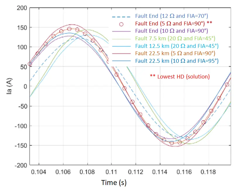
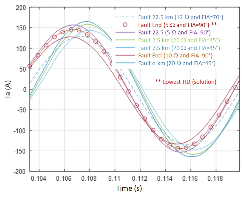
Figure 6a,b compare the test fault current (dashed line) with other fault current waveforms stored in the database for faults located at 25 km (end of the feeder) and 22.5 km, respectively. This suggests that each fault signal exhibits distinct characteristics and that, even with a small number of cases, identifying the closest signals would be nearly impossible without an appropriate similarity measure, such as the Hausdorff distance (HD). For illustration purposes, Figure 6 was elaborated using only the current signal from phase A.
 |
 |
|
(a) |
(b) |
Figure 6. Comparison between the test fault current waveform (dashed line) and the reference fault current waveforms stored in the database for the IEEE 5-bus system, considering: (a) faults applied at 25 km (end of the feeder) and (b) faults applied at 22.5 km from de feeder origin.
3.1.3. General Considerations on the Proposed Method
The findings presented in this section indicate that the proposed methodology is able to effectively identify the faulted region at different locations along the distribution feeder, thereby fulfilling the primary objective of this study.
It was observed that the method accurately identifies the faulted region when using sampling rates of 128 and 256 samples per cycle, but demonstrates poor performance at 64 samples per cycle. Regarding the data window length, no significant difference was observed between using one or two cycles of fault current (either for the test fault and the recorded samples). Therefore, to ensure the simplest and most efficient implementation, the proposed method is applied and tested throughout this work using 128 samples per cycle and a data window of one cycle. As will be shown, this configuration effectively achieves the goal of identifying faults along the feeder, regardless of fault characteristics or grid operating conditions. It is also worth noting that the method’s performance improves as the size of the database increases, which can be dynamically expanded over time.
It should be emphasized that, in the proposed methodology, the HD is not intended to establish a direct relationship with individual fault parameters, such as fault resistance, fault inception angle, or feeder location. Instead, HD is employed exclusively as a waveform similarity metric to compare a fault current measured in the field with a database of previously simulated or registered fault currents. Therefore, the effectiveness of the proposed method relies on the ability of the database to adequately represent the range of expected fault scenarios, rather than on a deterministic mapping between HD values and specific fault electrical parameters.
The main objective of this section was to highlight the potential of the proposed method despite the simplicity of its underlying concept. For validation purposes, the next section evaluates the proposed method on a second, more complex electrical system widely recognized by the technical community.
4. Validating the Proposed Method
The proposed method is tested against the IEEE 34-bus system, whose single-line diagram is illustrated in Figure 7. The network operates with a nominal frequency of 60 Hz and a distribution voltage of 24.9 kV, with multiphase loads, either balanced and unbalanced. The main features of this network are:
-
-
Overhead single- and three-phase distribution lines;
-
-
Single-phase voltage regulators between buses 814–850 and 832–852;
-
-
Shunt capacitor banks located at buses 844 and 848;
-
-
Autotransformer connected between buses 832 and 888, with a 24.9/4.16 kV ratio;
-
-
The existence of centralized (spot) and distributed loads.
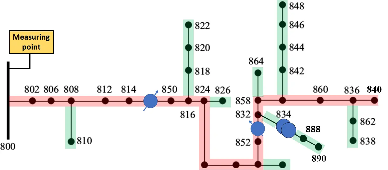
For analysis purposes, the system is divided into two parts, according to Figure 7. The first (in red) corresponds to the main three-phase section, while the second (in green) includes the single-phase and two-phase lateral sections.
To construct the database, a large number of fault scenarios were simulated under various operating conditions and fault characteristics, by varying the fault location, fault parameters (resistance and inception angle), and loading levels. For each scenario, a data window of one cycle and 128 samples per cycle is considered, and the resulting fault current waveform is stored in the database and associated with a specific location along the feeder.
4.1. Effect of System Load Variation
To test the method under more comprehensive and practical conditions, the loads had their active and reactive power reduced by 50% and 70%. The objective of this variation was to verify the impact of the loading system on the performance of the proposed method and to identify possible limits of its operation. Three cases were considered: (1) nominal loading; (2) 50% of the nominal load; (3) 70% of the nominal load.
4.1.1. Analysis Criteria
Single-phase faults were simulated at multiple locations along the distribution feeder, considering variations in both fault impedance and fault inception angle. As before, once a fault occurs, the fault current waveform at bus 800 is stored and then compared with a historical database using the HD method. Since approximately 85% of faults in distribution systems are single-phase, they are the main concern for electric utilities and therefore the primary focus of this study [22].
Unlike the previous tests, which used only the phase-A current waveform to calculate the HD, this section analyzes combinations of voltage and current waveforms from all phases, as illustrated in Figure 8. The input signals are labeled according to the waveform(s) used to compute the HD, as follows: HD Ia (phase-a current waveform), HD Va (phase-a voltage waveform), HD Iabc (three-phase current waveforms), and HD IabcVabc (combination of three-phase voltage and current waveforms).
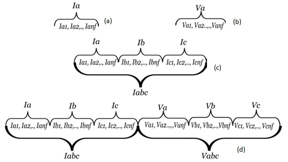
Figure 8. Input vectors employed to calculate the HD, where: (a) HD Ia; (b) HD Va; (c) HD Iabc; and (d) HD IabcVabc.
By considering different load conditions and fault locations, both in the main feeder and in the lateral branches, the accuracy and robustness of the proposed method were verified using the IEEE 34-bus system. It is worth noting that the test fault cases were simulated using fault parameters that are not represented in the constructed database, as indicated in Table 5.
Table 5. Parameter used for database construction and test case generation.
|
Database |
Tests |
|
|---|---|---|
|
FR (Ω) |
7, 12, 18, 25, 30 |
2.5, 5.5, and 7.5 |
|
FIA (°) |
10, 15, 30, and 70 |
20, 50, and 80 |
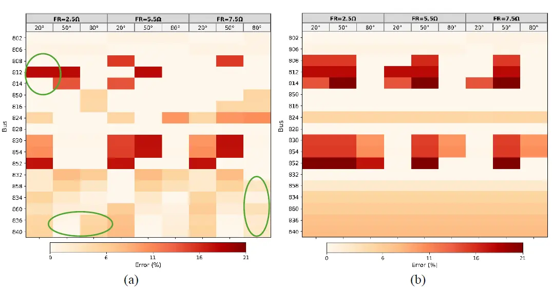
Table 6 presents the results of the proposed method for each input signal configuration, considering different sampling rates and data window sizes. This analysis supports selecting an appropriate configuration to implement an accurate fault-region identification scheme in distribution systems. As observed from the results, the best trade-off between performance and simplicity is achieved with a configuration of 128 samples per cycle and a data window size of one cycle. To illustrate how this configuration performs with different input signals, Figure 9 presents the method’s results, represented as heatmaps derived from Equation (5), for a large number of fault cases. The database comprises 360 cases (5 fault resistances × 4 fault inception angles × 18 fault locations), while 162 additional cases (3 fault resistances × 3 fault inception angles × 18 fault locations) are used for testing.
As shown in Figure 9, when the input signals Ia and Iabc are used, the proposed method exhibits better performance compared with the cases employing Va and IabcVabc. It is also important to note that, in general, between Ia and Iabc, the latter provides slightly superior performance, as illustrated in the figure.
Table 6. Number of test fault cases correctly identified for different input signals and configuration parameters.
|
Input Signal |
Sample by Cycle/Data Window Size |
||||
|---|---|---|---|---|---|
|
128/1 |
128/2 |
256/1 |
256/2 |
Average |
|
|
Ia |
63 |
63 |
66 |
60 |
63 |
|
Va |
44 |
44 |
48 |
49 |
46.25 |
|
Iabc |
68 |
73 |
62 |
51 |
63.5 |
|
IabcVabc |
59 |
59 |
62 |
58 |
59.5 |
 |
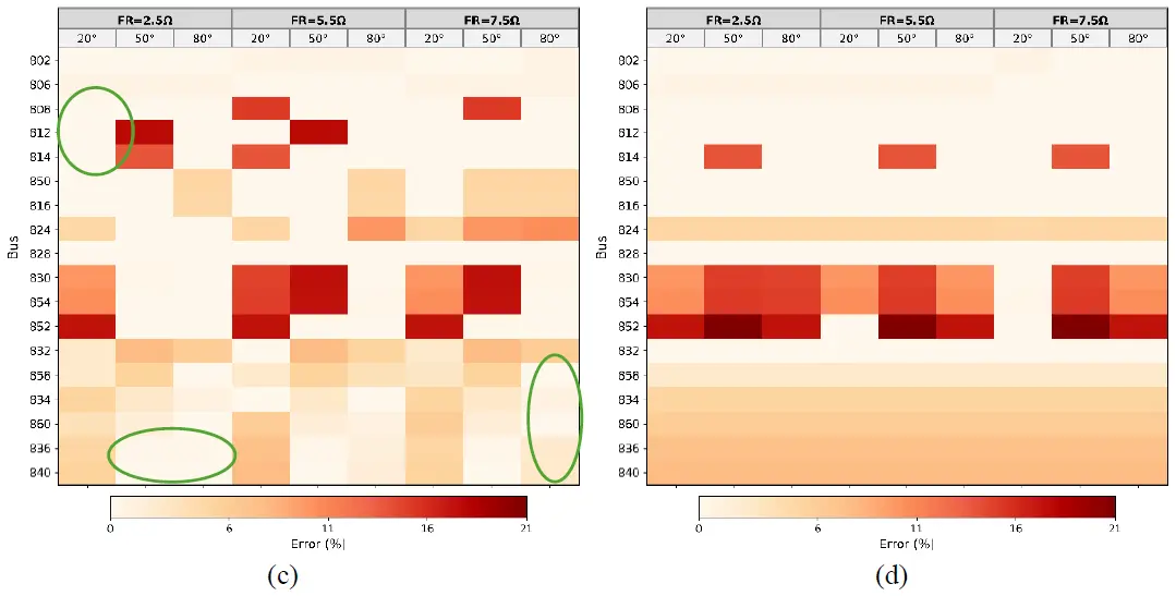 |
Figure 9. Percentage error distribution by bus location (vertical axis) as a function of fault resistance, and inception angle (horizontal axes) for the following input signals: (a) Ia, (b) Va, (c) Iabc, and (d) IabcVabc ($${t}_{A}=128$$ and $${n}_{j}=1$$).
To evaluate the method’s performance under different operating conditions, the tests were repeated with 70% and 50% of the nominal load, considering the two best-performing input signals identified in the previous analysis, namely the current waveforms Ia (Figure 10a,c) and Iabc (Figure 10b,d). The results suggest a weak correlation between fault location estimation errors and load levels. The observed variations are mainly attributed to the different input signal waveforms used. The number of test fault cases correctly identified for each operating condition is presented in Table 7.
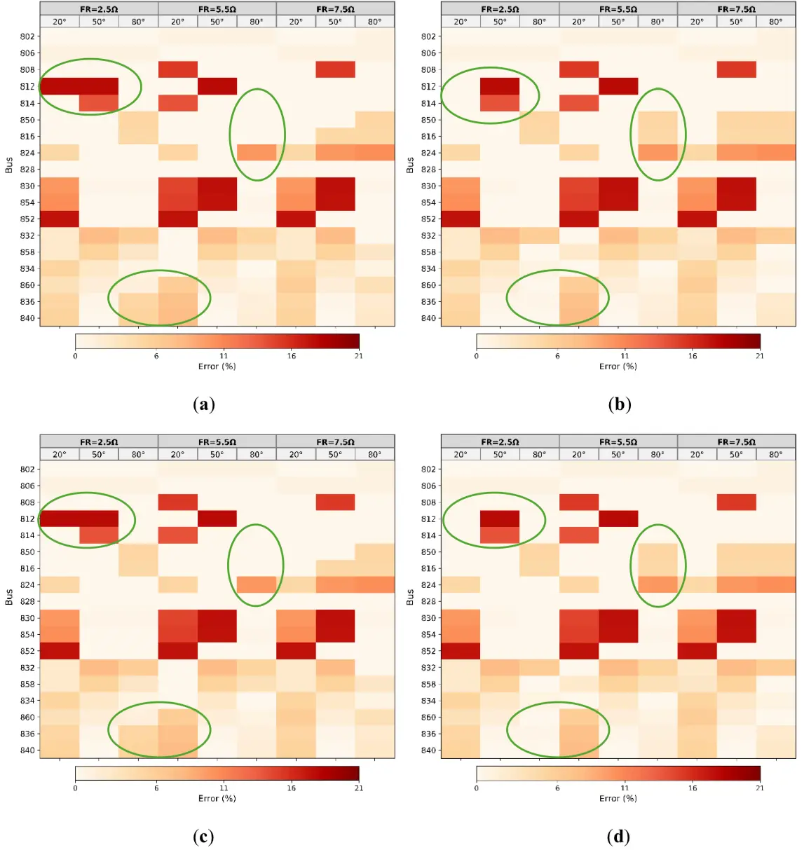
Figure 10. Percentage error distribution by bus location (vertical axis) as a function of fault resistance and inception angle (horizontal axes) for different input signals and load levels: (a) Ia, 70% load; (b) Iabc, 70% load; (c) Ia, 50% load; and (d) Iabc, 50% load.
Table 7. Number of test faults correctly identified, by input signal and loading levels.
|
Input Signals |
100% of Nominal Load |
70% of Nominal Load |
50% of Nominal Load |
Total |
|---|---|---|---|---|
|
Ia |
63 |
62 |
63 |
188 |
|
Va |
44 |
44 |
44 |
132 |
|
Iabc |
68 |
68 |
68 |
204 |
|
IabcVabc |
59 |
59 |
58 |
176 |
Another important aspect of the evaluation concerns the impact of the database size on the method’s performance. To this end, the database was expanded using the parameters listed in Table 8, considering only single-phase faults, given their prevalence in distribution systems. As shown in Table 8, combining the new values assigned to each variable yields dataset DB-1, comprising 1584 fault cases, and dataset DB-2, comprising 6336 fault cases, thereby enabling a more comprehensive analysis. Using the values presented in the last column of Table 8, new test cases were generated to evaluate the performance of the proposed method.
Table 8. Parameter used to construct new databases and test cases.
|
DB-1 |
DB-2 |
Test |
|
|---|---|---|---|
|
FR (Ω) |
1, 3, 7, 12, 16, 18, 20, 23, 25, 28, and 30 |
0, 1, 3, 5, 7, 12, 14, 16, 18, 20, 23, 25, 26, 28, 30, 35, 38, 40, 45, 50, 55, and 60 |
2, 15, and 27 |
|
Fault Inception Angle—FIA (°) |
10, 15, 25, 30, 50, 70, 75, and 85 |
3, 5, 10, 12, 15, 18, 25, 30, 45, 50, 60, 70, 75, 78, 85, and 90 |
20, 40, and 80 |
After completing all simulations and tests, the results were compiled and summarized in Table 9, which, as in the previous analyses, presents the fault location estimation error for fault cases occurring along the main feeder from bus 802 to bus 840. To comprehensively assess the impact of the database size on the method’s performance, a total of 324 test fault cases were evaluated (18 buses × 3 fault resistances × 3 fault inception angles × 2 databases). It is important to emphasize that the primary purpose of this table (and its correspondent heatmaps) is to illustrate the influence of the database size on the accuracy of the proposed solution by comparing the color patterns across the heatmaps, while the variable axes are maintained the same for all analyzed cases. The results show that the database size has a significant impact on the method’s performance. The performance obtained using datasets DB-1 and DB-2 was generally improved compared with that achieved using the previous database containing 360 fault cases (see Table 5, Figure 9 and Figure 10). Moreover, in general, DB-2 yielded more accurate results than DB-1, indicating that larger databases lead to higher fault-location accuracy. Also, it can be observed that DB-2 renders the method independent of the load condition.
Table 9. Comparison of fault location accuracy between BD-1 and BD-2 under 70% and 100% load conditions for input signals Ia and Iabc.
|
Load Condition |
Input Signals for FR [2 Ω; 15 Ω; 27 Ω] and FIA [20°; 40°; 80°] |
||
|---|---|---|---|
|
Ia |
Iabc |
||
|
100% |
BD-1 |
|
|
|
BD-2 |
|
|
|
|
70% |
BD-1 |
|
|
|
BD-2 |
|
|
|
|
50% |
BD-1 |
|
|
|
BD-2 |
|
|
|
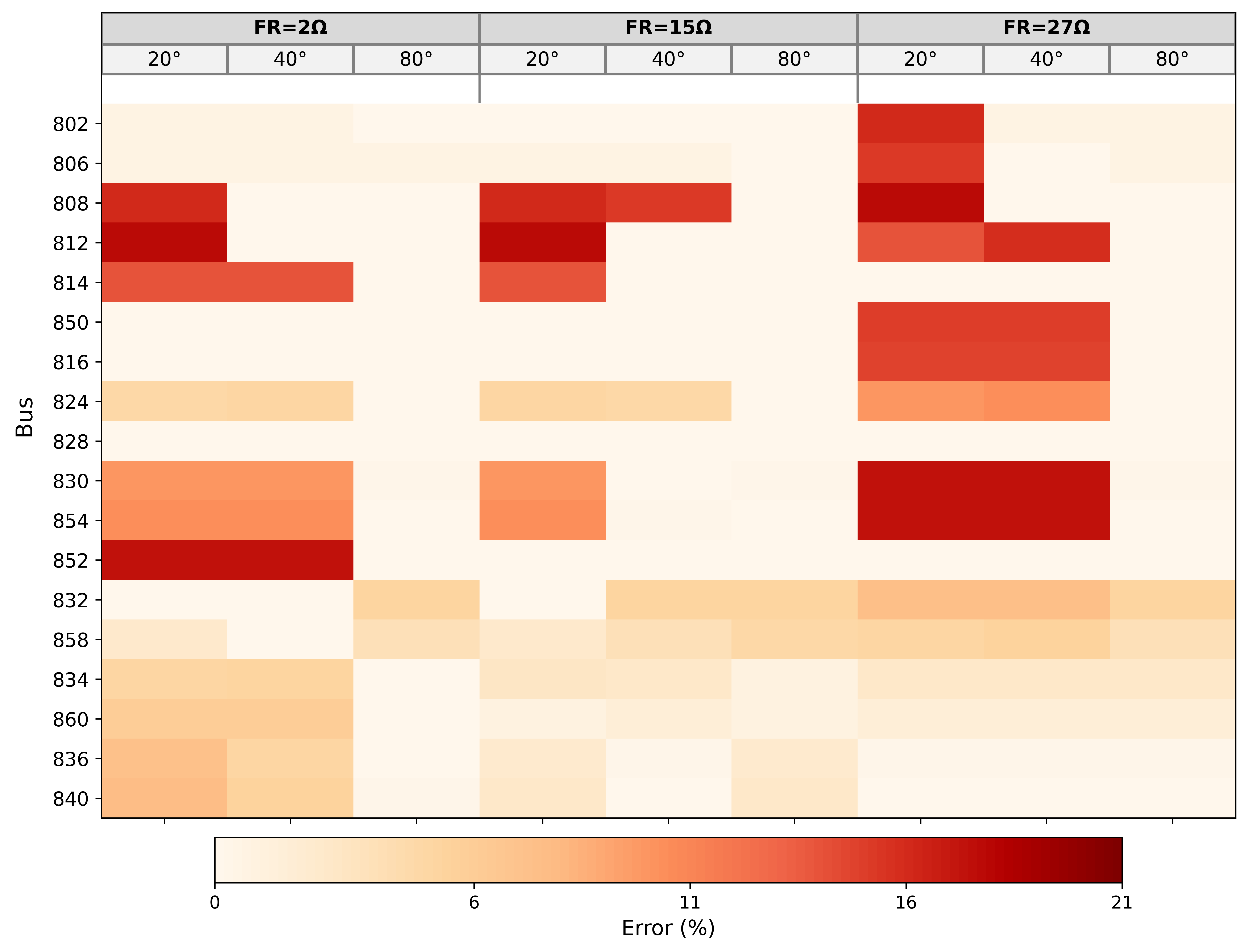
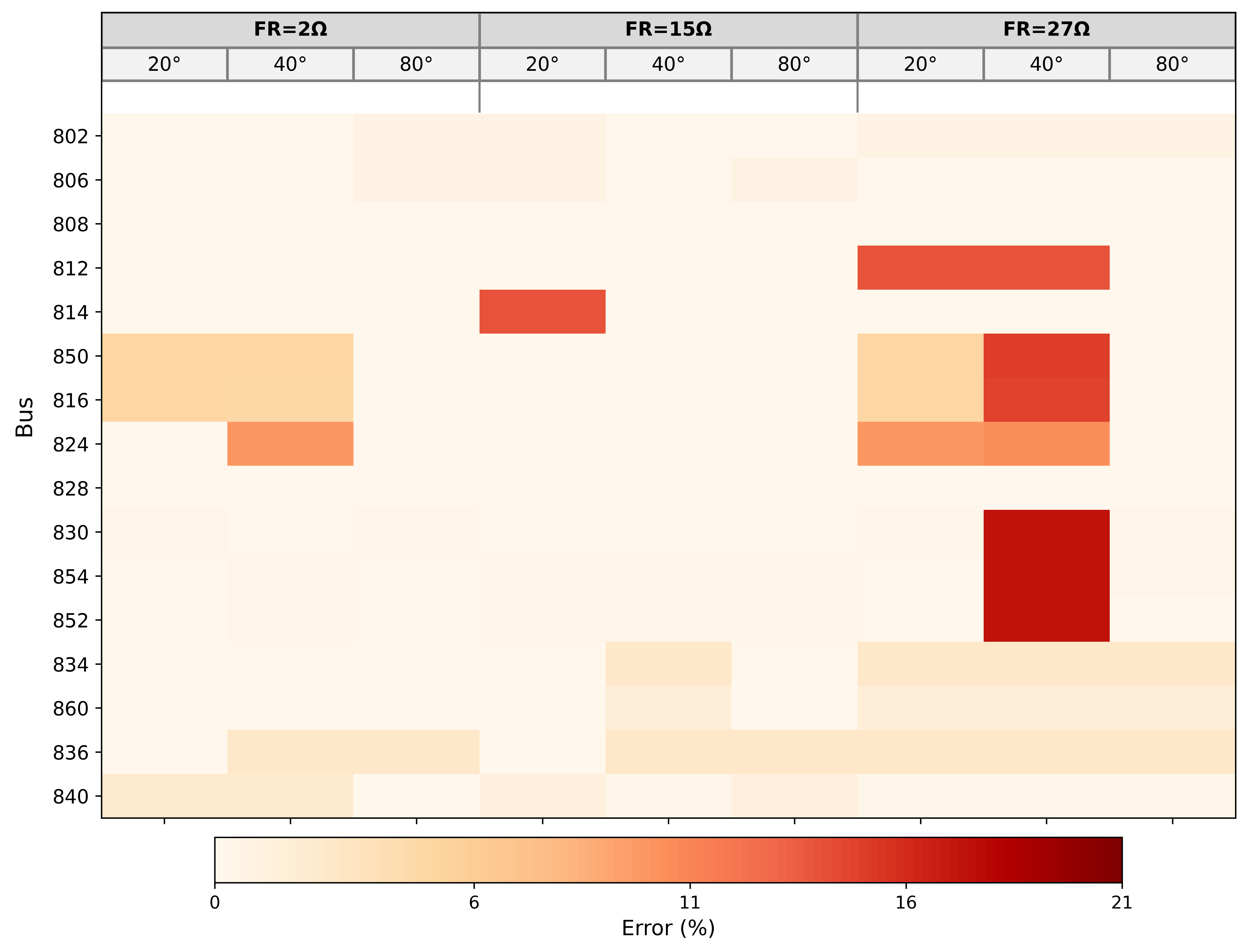
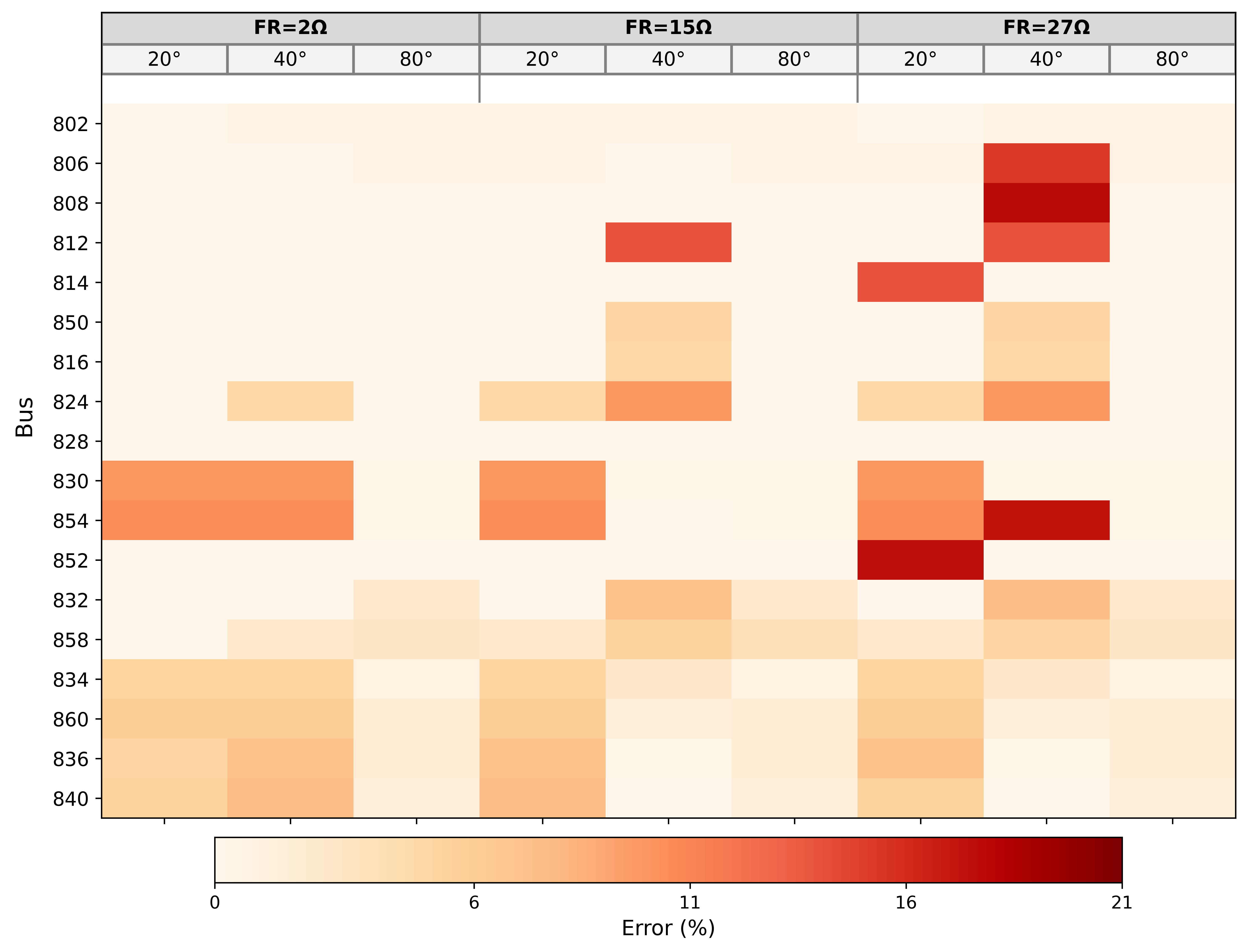
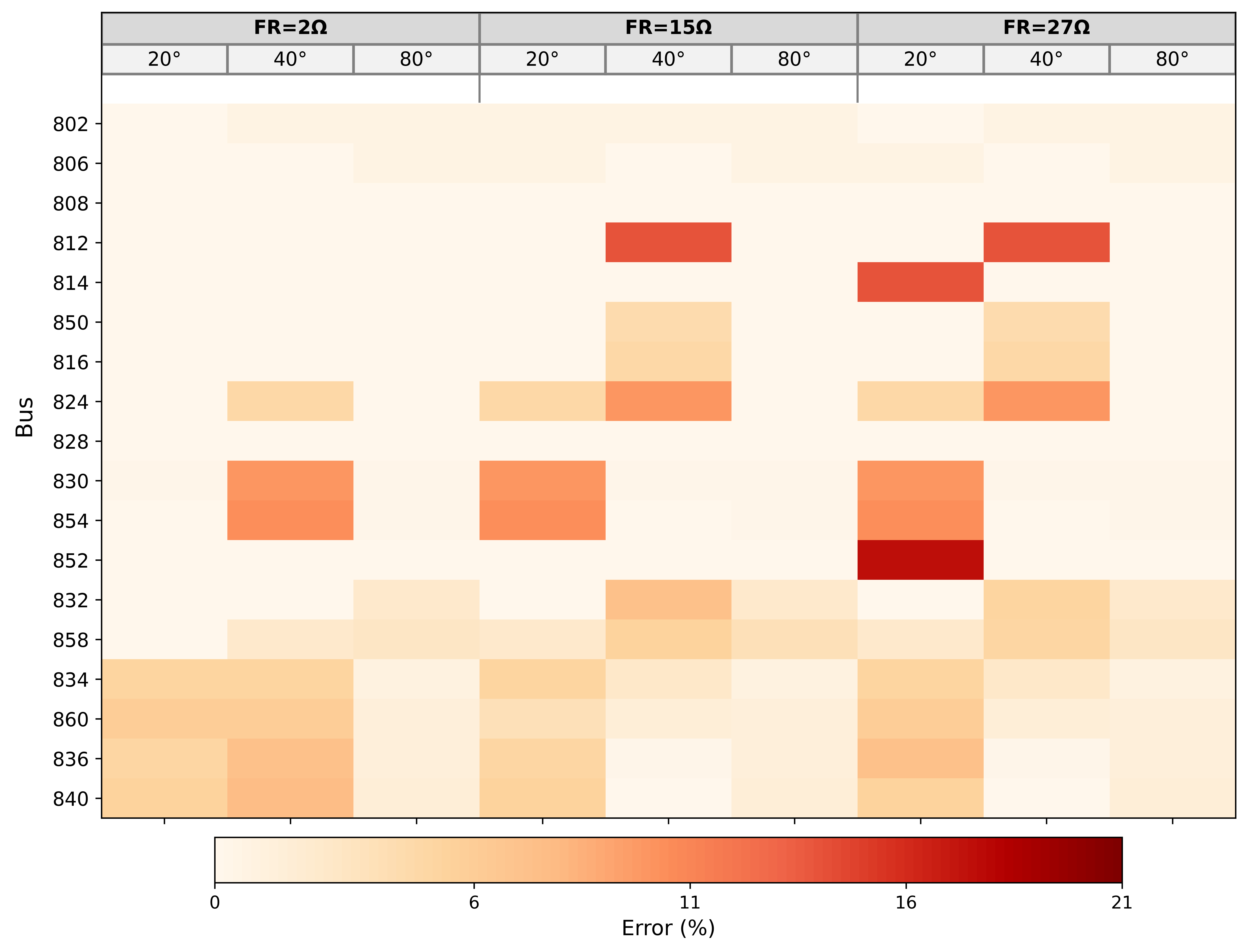
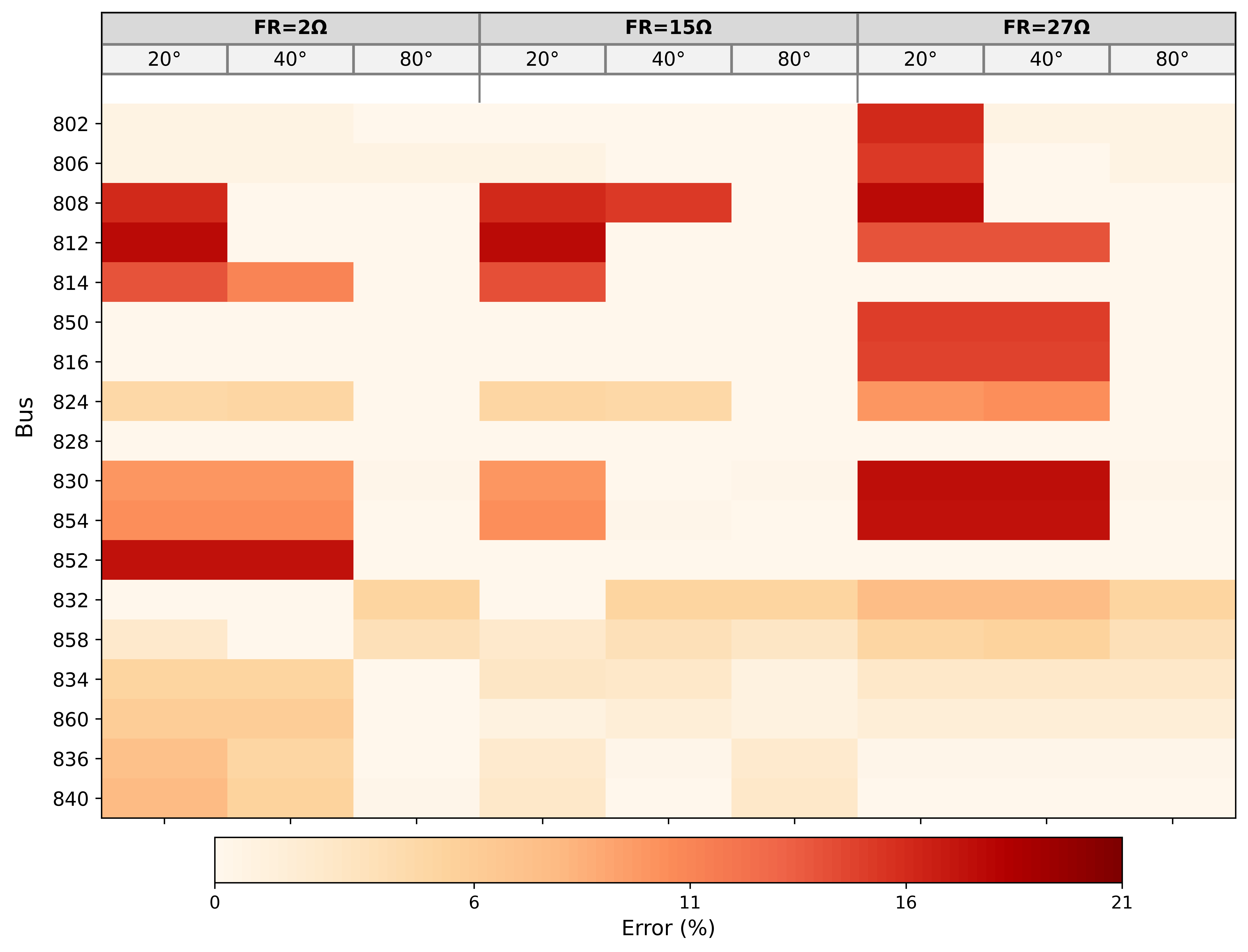
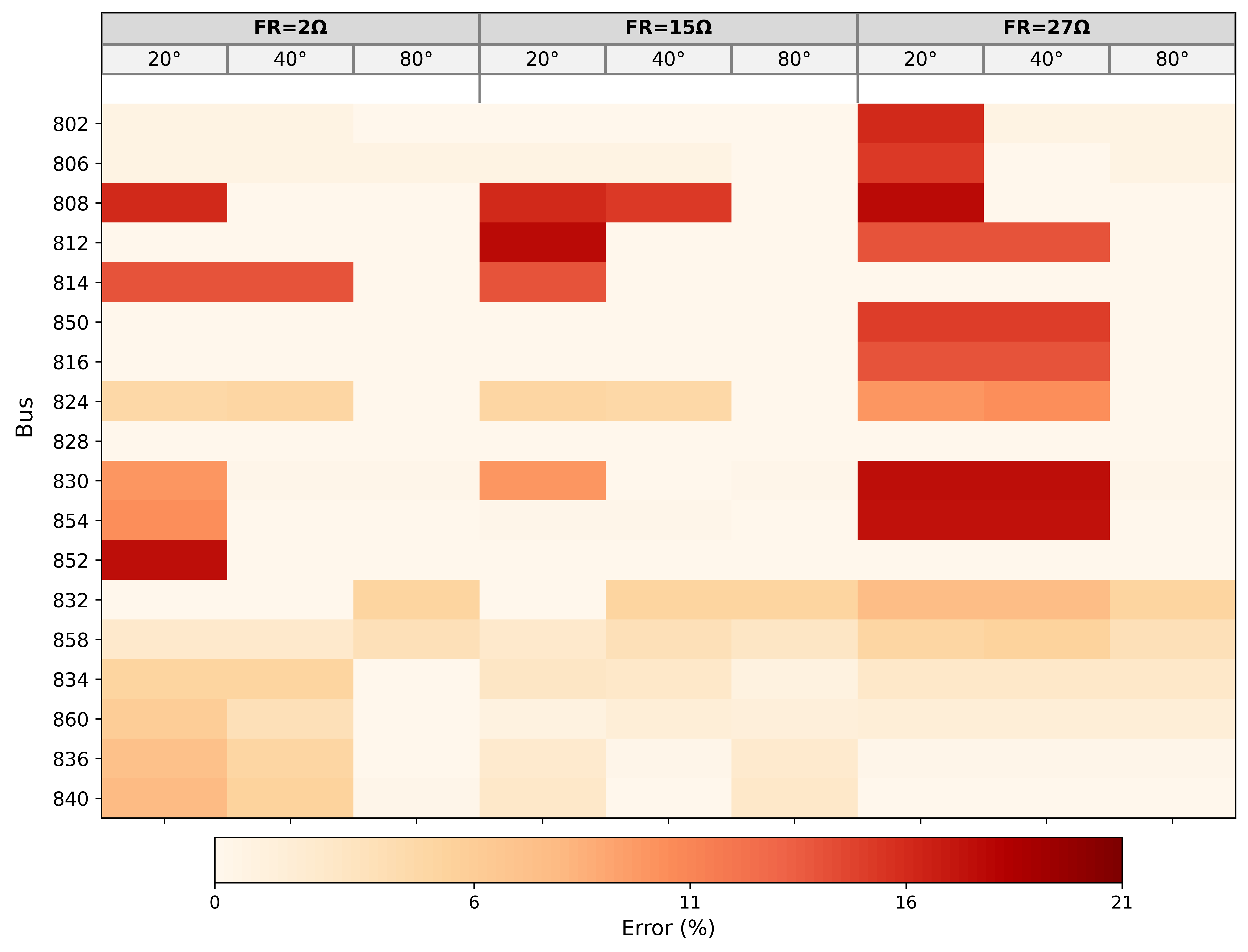
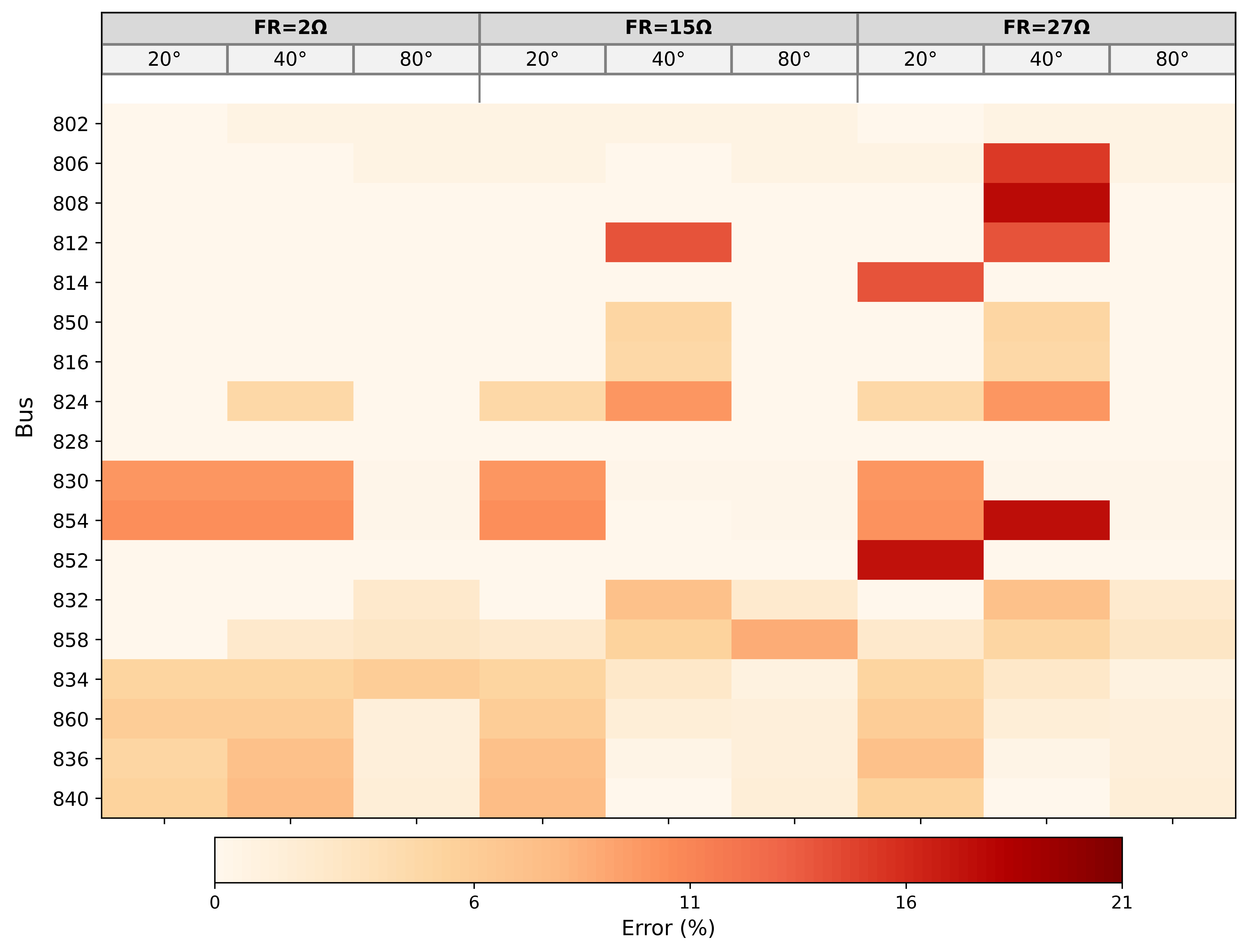
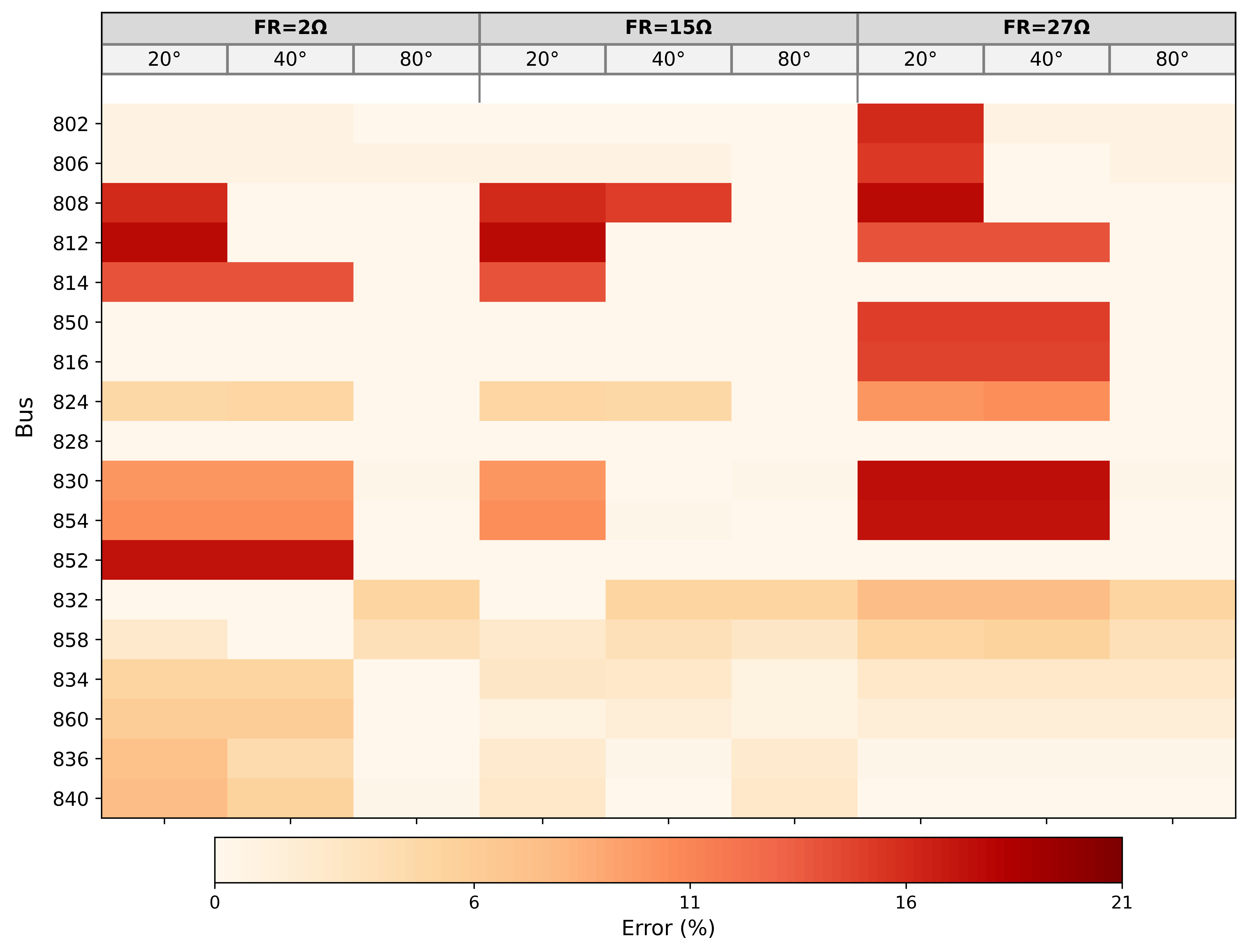
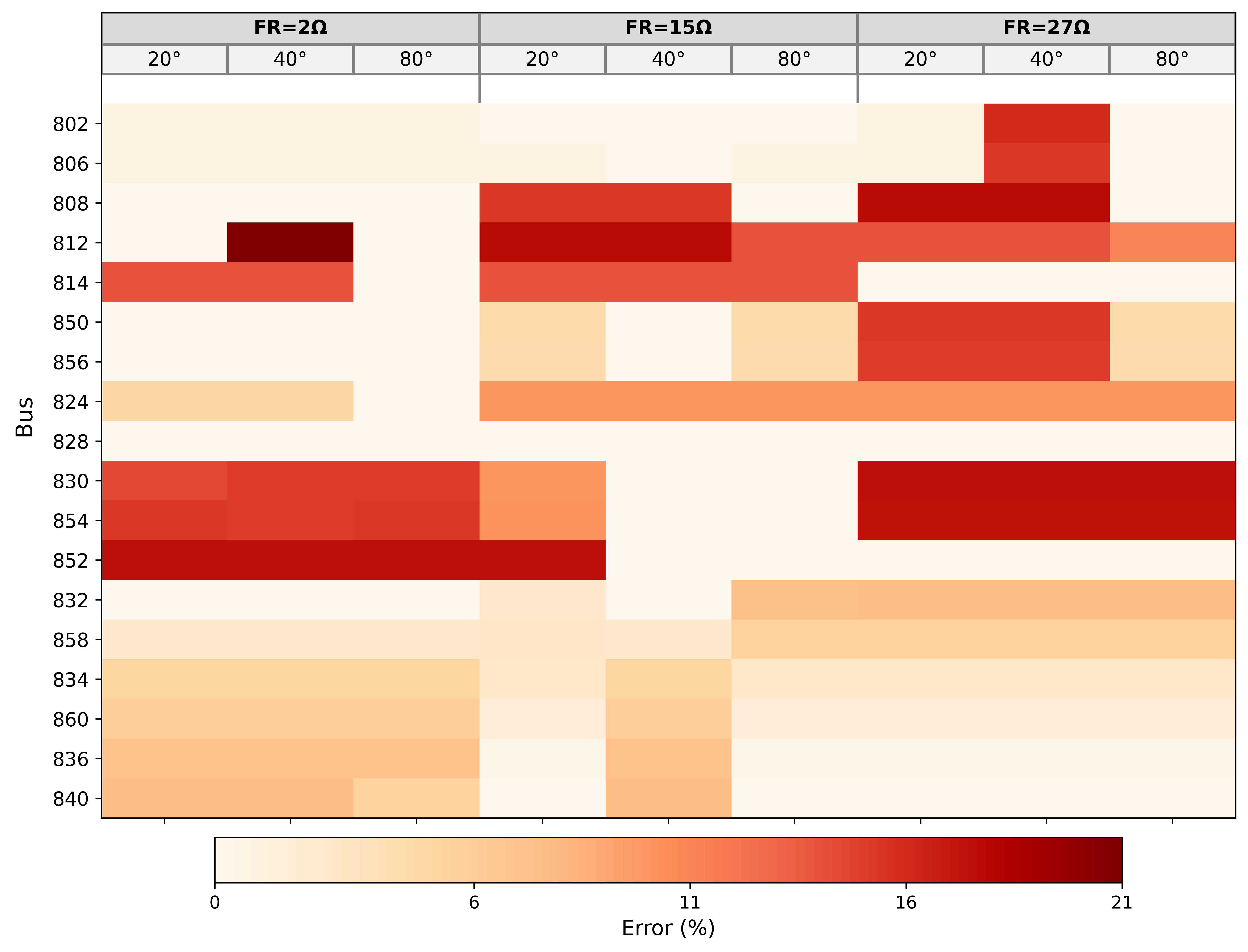
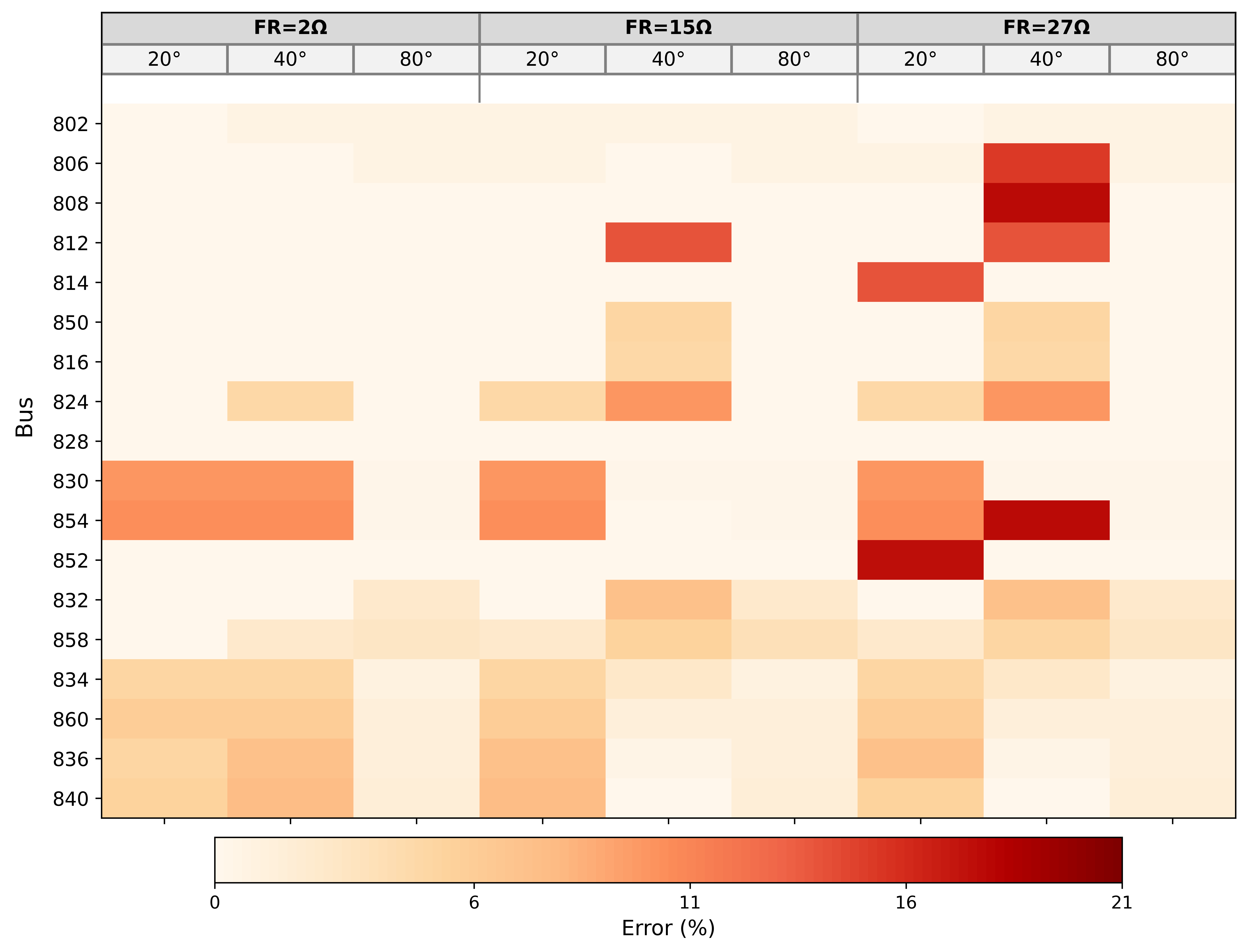
Note: In each figure, the vertical axis represents the bus location, while the primary horizontal axis represents the fault resistance values (2 Ω, 15 Ω, and 27 Ω), and the secondary horizontal axis represents the fault inception angle values (20°, 40°, and 80°).
Another important conclusion drawn from the observed results concerns the selection of the input signal. As can be observed, in most cases, the use of Iabc resulted in higher accuracy than Ia. Therefore, the configuration using Iabc as the input signal is adopted for the subsequent evaluations, considering the lateral branches, consistently maintaining 128 samples per cycle and a one-cycle data window, as previously discussed.
4.1.2. Evaluation of Faults in Lateral Branches
In this section, the proposed similarity-based method is evaluated for faults occurring along the lateral branches of the IEEE 34-bus system. Initially, a new database (DB-3) was constructed using the input signal Iabc, selected based on its previously demonstrated superior performance. An important aspect is that DB-3 contains fault signals only from the main feeder and does not include fault signals from the lateral branches. Consequently, the method is expected to identify the fault location in DB-3 that is closest to the fault point in the lateral branch. For this simulation, the FR and FIA parameters are those listed in Table 10, with test fault cases applied at buses 816, 818, 819p, 820, 821p, 822, 863p, and 864.
Table 10. Parameters variation to construct DB-3 and perform tests in lateral branches.
|
Values of the DB-3 |
Values for Test |
|
|---|---|---|
|
FR (Ω) |
0, 1, 3, 5, 7, 12, 14, 16, 18, 20, 23, 25, 26, 28, 30, 35, 38, 40, 45, 50, 55, and 60 |
2, 15 and 27 |
|
$$FIA$$ (°) |
3, 5, 10, 12, 15, 18, 25, 30, 45, 50, 60, 70, 75, 78, 85, and 90 |
20, 40, and 80 |
|
Location (bus) |
802, 806, 808, 812, 814, 850, 816, 824, 828, 830, 854, 852, 832, 858, 834, 860, 836, and 840 |
816, 818, 819p, 820, 821p, 822, 863, and 864 |
Figure 11 illustrates the poor performance of the method in this test scenario. In fact, regardless of the loading condition, the absence of fault cases in the lateral branches significantly reduces the accuracy of the proposed solution, since a sufficient level of similarity is not achieved between the faulted signal (from the field) and those stored in DB-3. As can be observed, since the method always provides discrete responses through a waveform pattern-matching approach, and the approximation error depends on the database size, all cases were similarly affected regardless of their operating conditions.
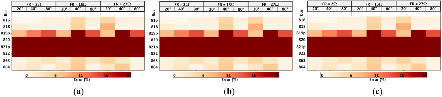
Figure 11. Fault location estimation errors for fault cases at buses of the lateral branches under different load levels using the Iabc input signal: (a) nominal load, (b) 70% load, and (c) 50% load.
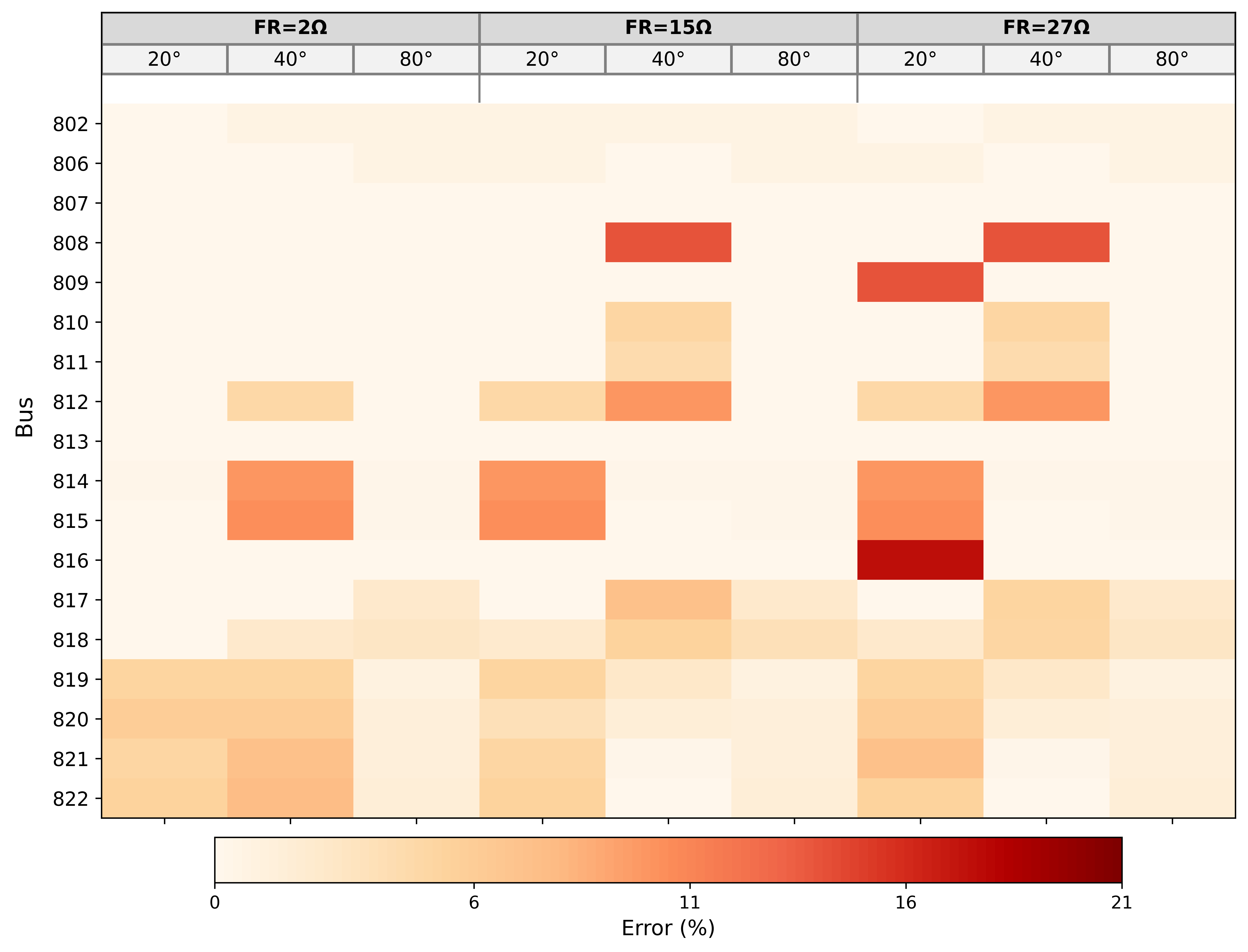
To address the previously identified issue of low accuracy for faults occurring in the lateral branches, the original DB-3 dataset was updated to include fault signals from the lateral branches. The final dataset includes fault records from both the main feeder and the lateral branches, expanding from 6336 to 9152 fault cases through the inclusion of different fault locations, FR, and FIA values, as previously defined in Table 10.
The simulation results are presented in Figure 12. As expected, once DB-3 is updated with the fault records from the newly introduced buses, a higher level of accuracy is reached, regardless of the operating condition. The results also confirm that using 128 samples per cycle and a one-cycle data window for computing the HD yields robust performance across the scenarios considered, as all evaluations consistently produced similar heatmaps.
Once again, it becomes evident that the method’s performance depends on the size of the database, which can be updated as needed to meet specific requirements and desired levels of accuracy. It should be noted that the proposed similarity-based method, which employs the HD, is simple and relies only on readily available resources (from simulations or historical field data). Moreover, it can serve as an important tool to help utility maintenance teams accurately identify faulted regions, thereby speeding system restoration and enhancing distribution system availability.
It should be noted that the results presented in this section are intended to illustrate the influence of database density on the performance of the proposed methodology rather than to establish a universal minimum database size. The optimal database configuration should be selected according to the requirements of each specific application, considering factors such as network characteristics, desired identification resolution, and computational constraints. Furthermore, the performance of the proposed approach is always evaluated in terms of correct identification of the faulted region rather than the absolute fault-distance error.
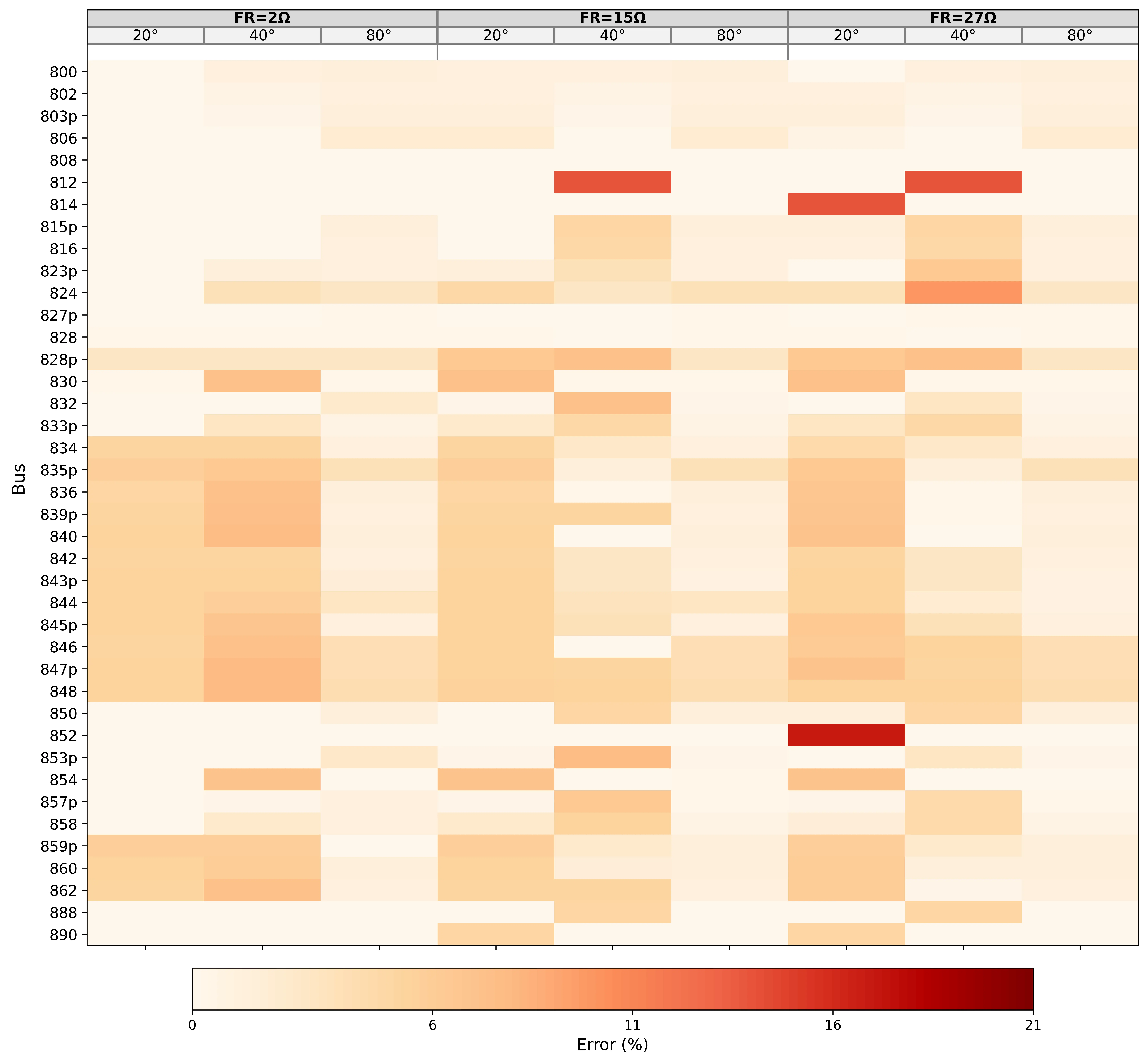
Figure 12. Percentage fault location estimation errors by bus location (vertical axis) and fault parameters (horizontal axes) for the Iabc input signal, evaluated using the extended DB-3 dataset (tA = 128, nj = 1, and nominal load).
4.1.3. Comparisons with Other Methods
Compared with the alternative approaches summarized in Table 11, the primary advantage of the proposed method is its computational simplicity. The method quantifies the similarity between electrical signals using HD to identify the faulted region and relies solely on simple mathematical operations applied directly to the sampled current, without requiring any complex preprocessing stage. Moreover, the method performs well at low sampling frequencies, reducing the requirements imposed on existing hardware and making it readily applicable in real-world scenarios.
As shown in Table 11, approaches with different complexity levels offer distinct capabilities and can address different fault scenarios depending on the required accuracy. The solution proposed in this work provides an acceptable trade-off between simplicity and performance, supporting operators in routine tasks while enabling rapid identification of fault regions and timely restoration of the distribution system.
In general terms, the main advantage of the proposed method is its ability to support utility maintenance teams without requiring additional investment, as it relies solely on available resources and appropriate processing of fault current waveforms. As shown in Table 11, other methods that achieve higher robustness generally require higher sampling frequencies, communication links, and more complex signal processing schemes, which may limit their practical applicability.
Table 11. Comparison of the proposed method with other works.
|
References |
Input Signal |
Algorithm |
Fault Resistance (Ω) |
Complexity |
Sampling Frequency (Hz) |
Test System |
Commun. Link |
|---|---|---|---|---|---|---|---|
|
Proposed Method |
I |
Hausdorff Distance |
30 |
Low |
7680 |
(a) 5-bus system (b) IEEE 34-bus |
No |
|
[6] |
V and I |
Artificial Neural Network |
0 |
Moderate |
50,000 |
Real power grid modeled in Matlab |
No |
|
[17] |
I |
Hausdorff Distance |
1000 |
Moderate |
10,000 |
Typical 10 kV power grid |
Yes |
|
[8] |
V and I |
Impedance matrix |
50 |
High |
Not mentioned |
(a) Hypothetical power grid (b) IEEE 37-bus |
Yes |
|
[20] |
I |
Normalized Hausdorff Distance |
1000 |
High |
10,000 |
(a) 10 kV radial system (b) IEEE 33-bus |
Yes |
It should be noted that the methods summarized in Table 11 were developed for different distribution systems, datasets, fault scenarios, and evaluation criteria. Therefore, a direct quantitative comparison of performance metrics is not possible. The purpose of this comparison is to highlight the methodological differences and practical contributions of the proposed approach with respect to related studies, rather than to establish a benchmark under identical experimental conditions.
4.1.4. Final Considerations
After an extensive evaluation, the final configuration of the proposed method (three-phase currents (Iabc), sampling rate of 128 samples per cycle, and one-cycle data window) was found to be insensitive to load variations but sensitive to the sampling rate, data window size, and database construction. In addition, the method demonstrated robustness to variations in fault resistance and fault inception angle. When the objective is limited to identifying faulted regions in the main feeder, either the phase-A current (Ia) or the three-phase currents (Iabc) can be used interchangeably, although Ia results in a lower computational burden. However, when faulted region identification in the lateral branches is also required, the three-phase currents (Iabc) constitute the more suitable input, providing higher accuracy at the expense of increased computational cost.
As demonstrated, the accuracy of faulted region identification mainly depends on the comprehensiveness of the database. Therefore, it is possible to create a general database representing the original power system configuration, as well as secondary databases representing the distribution system under different network configurations resulting from topology changes, for example, after switching operations.
The proposed methodology is intended for offline post-fault analysis, where oscillographic records obtained after fault occurrence are compared with a database of previously simulated or recorded fault waveforms. Therefore, it can be periodically expanded and refined offline as new fault records become available, allowing utilities to tailor its size and coverage according to network characteristics, operational requirements, and maintenance policies.
Considering all the evaluations performed in this study, the favorable trade-off between performance and implementation cost makes the proposed method an attractive and readily applicable solution for supporting engineers responsible for power system operation.
5. Conclusions
This paper presents a method for identifying the faulted region in distribution systems. The method was initially developed and evaluated using a small system with distributed generation and was subsequently applied to a larger distribution network to validate its effectiveness and demonstrate its applicability.
Several input signals, sampling rates, and data window lengths were evaluated to determine the most suitable configuration for the proposed method. The selected configuration was capable of identifying the faulted region under varying load conditions, fault inception angles, and fault resistances. In addition, the proposed method was found to be insensitive to load variations but strongly dependent on the size and completeness of the database, which can be readily updated to meet the specific requirements of a given distribution system.
A key characteristic of the proposed HD-based fault region identification method is its simplicity: it relies solely on basic mathematical operations and incurs low computational cost. The method requires only existing, readily available infrastructure, offering a promising low-cost solution without additional IEDs or communication networks. Consequently, it can assist utility operators by rapidly identifying the faulted region, thereby facilitating fault isolation and service restoration.
As future work, the proposed method could be evaluated in larger and more complex modern distribution systems with a high penetration of converter-interfaced renewable energy sources. In addition, its performance could be investigated under high levels of measurement noise and high-impedance fault conditions, in which the fault and load currents are often very similar.
This study focuses exclusively on single-phase-to-ground faults because they represent the vast majority of fault events in distribution systems and therefore constitute the primary application of interest for the proposed methodology. Extending the database and validation procedure to include two-phase, two-phase-to-ground, and three-phase faults is also left as future work.
Acknowledgments
The authors would like to thank the Coordination for the Improvement of Higher Level Personnel (CAPES) and the Ministry of Education of Brazil for its financial support, and also the National Institute of Science and Technology of Electric Energy-Brazil (INCT-INERGE).
Author Contributions
Conceptualization, R.C.d.S. and J.S.d.L.; Methodology, R.C.d.S. and J.S.d.L.; Software, E.W.S.d.Â. and J.S.d.L.; Validation, E.W.S.d.A. and J.S.d.L.; Formal Analysis, R.C.d.S. and E.A.B.; Investigation, J.S.d.L.; Data Curation, J.S.d.L.; Writing—Original Draft Preparation, R.C.d.S., E.W.S.d.Â. and E.A.B.; Writing—Review & Editing, G.T.d.A., A.M.d.S. and R.C.d.S.; Visualization, J.S.d.L., G.T.d.A. and A.M.d.S.; Supervision, R.C.d.S.
Ethics Statement
Not applicable.
Informed Consent Statement
Not applicable.
Data Availability Statement
The data supporting the findings of this study are not publicly available.
Funding
This research was funded by CAPES Brazil, Finance Code 001.
Declaration of Competing Interest
The authors declare that they have no known competing financial interests or personal relationships that could have appeared to influence the work reported in this paper.
References
- Dashtdar M, Dashtdar M. Fault Location in Radial Distribution Network Based on Fault Current Profile and the Artificial Neural Network. Sci. Bull. Electr. Eng. Fac. 2020, 20, 14–21. DOI:10.2478/sbeef-2020-0103 [Google Scholar]
- Liang J, Jing T, Niu H, Wang J. Two-Terminal Fault Location Method of Distribution Network Based on Adaptive Convolution Neural Network. IEEE Access 2020, 8, 54035–54043. DOI:10.1109/ACCESS.2020.2980573 [Google Scholar]
- Shi X, Xu Y. A fault location method for distribution system based on one-dimensional convolutional neural network. In Proceedings of the 2021 IEEE International Conference on Power, Intelligent Computing and Systems (ICPICS), Shenyang, China, 29–31 July 2021; pp. 333–337. DOI:10.1109/ICPICS52425.2021.9524222 [Google Scholar]
- Yu Y, Li M, Ji T, Wu QH. Fault location in distribution system using convolutional neural network based on domain transformation. CSEE J. Power Energy Syst. 2021, 7, 472–484. DOI:10.17775/CSEEJPES.2020.01620 [Google Scholar]
- Zhou C, Gui S, Liu Y, Ma J, Wang H. Fault Location of Distribution Network Based on Back Propagation Neural Network Optimization Algorithm. Processes 2023, 11, 1947. DOI:10.3390/pr11071947 [Google Scholar]
- Awasthi S, Singh G, Ahamad N. Identification of type and location of a fault in a Distributed Generation System. Int. J. Comput. Digit. Syst. 2023, 14, 39–48. DOI:10.12785/ijcds/140104 [Google Scholar]
- Hong FK, Wong JKR, Heong OK, Kuan TM. Fault Classification and Location for Distribution Generation Using Artificial Neural Networks. In Proceedings of the 2020 IEEE International Conference on Power and Energy (PECon), Penang, Malaysia, 7–8 December 2020; pp. 315–320. DOI:10.1109/PECon48942.2020.9314535 [Google Scholar]
- Hosseinimoghadam SMS, Dashtdar M, Dashtdar M. Fault Location in Distribution Networks with the Presence of Distributed Generation Units Based on the Impedance Matrix. J. Inst. Eng. India Ser. B 2021, 102, 227–236. DOI:10.1007/s40031-020-00520-2 [Google Scholar]
- Lucas F, Costa P, Batalha R, Leite D, Škrjanc I. Fault detection in smart grids with time-varying distributed generation using wavelet energy and evolving neural networks. Evol. Syst. 2020, 11, 165–180. DOI:10.1007/s12530-020-09328-3 [Google Scholar]
- Sun Z, Wang Q, Wei Z. Fault location of distribution network with distributed generations using electrical synaptic transmission-based spiking neural P systems. Int. J. Parallel Emergent Distrib. Syst. 2021, 36, 11–27. DOI:10.1080/17445760.2019.1682145 [Google Scholar]
- Hou S, Han S. Fault location in distribution network based on discrete Fréchet distance algorithm. In Proceedings of the 2017 9th International Conference on Advanced Infocomm Technology (ICAIT), Chengdu, China, 22–24 November 2017; pp. 44–410.1109/ICAIT.2017.8388886 [Google Scholar]
- Luo H. Fault section location method for distribution network based on waveform difference clustering. J. Phys. Conf. Ser. 2023, 2530, 012012. DOI:10.1088/1742-6596/2530/1/012012 [Google Scholar]
- Prasad CD, Nayak PK. A DFT-ED based approach for detection and classification of faults in electric power transmission networks. Ain Shams Eng. J. 2019, 10, 171–178. DOI:10.1016/j.asej.2018.02.004 [Google Scholar]
- Alencar GT, Santos RC, Neves A. Euclidean Distance-Based Method for Fault Detection and Classification in Transmission Lines. J. Control. Autom. Electr. Syst. 2022, 33, 1466–1476. DOI:10.1007/s40313-022-00918-x [Google Scholar]
- Huttenlocher DP, Kedem K. Computing the minimum Hausdorff distance for point sets under translation. In Proceedings 10.1145/98524.98599 [Google Scholar]
- Zhao J, Zhang G, Shi X, Shi W. Fault section location method using wide area centralized structure based on modified Hausdorff distance. In Proceedings of the 2017 IEEE Conference on Energy Internet and Energy System Integration (EI2), Beijing, China, 26–28 November 2017; pp. 1–6. DOI:10.1109/EI2.2017.8245372 [Google Scholar]
- Chen Y, Wang L, Ji H, Wang J, Yu X, Gu J. Fault location of multistage feeders in distribution network. In Proceedings of the 2019 4th International Conference on Intelligent Green Building and Smart Grid (IGBSG), Yichang, China, 6–9 September 2019; pp. 49–10.1109/IGBSG.2019.8886231 [Google Scholar]
- Zhou W, Li Y, Guo Y, Qiao X, Deng W. Daily Maximum Load and Its Occurrence Time Forecasting of Distribution Network Based on Hausdorff Distance and ElasticNet. In Proceedings of the 2021 3rd Asia Energy and Electrical Engineering Symposium (AEEES), Chengdu, China, 26–29 March 2021; pp. 674–678. DOI:10.1109/AEEES51875.2021.9403105 [Google Scholar]
- Maiseli BJ. Hausdorff Distance with Outliers and Noise Resilience Capabilities. SN Comput. Sci. 2021, 2, 358. DOI:10.1007/s42979-021-00737-y [Google Scholar]
- Zhang G, Xiao G, Liu X, Xu Y, Wang P. Robust Faulted Line-section Location for Distribution Networks Based on Normalized Quantile Hausdorff Distance. J. Mod. Power Syst. Clean Energy 2026, 14, 273–285. DOI:10.35833/MPCE.2024.001299 [Google Scholar]
- Liang Y, Chen H, Sui S. Adaptive Current Differential Protection Method Based on the Hausdorff Distance Algorithm. In Proceedings of the 2024 IEEE 7th International Conference on Information Systems and Computer Aided Education (ICISCAE), Dalian, China, 27–29 September 2024; pp. 497–501. DOI:10.1109/ICISCAE62304.2024.10761675 [Google Scholar]
- Wu W, Zhang PX, Qiao D, Sun Q, Wang W. A Faulty Feeder Selection Method based on Improved Hausdorff Distance Algorithm for Neutral Non-effectively Grounded System. Electr. Power Syst. Res. 2022, 203, 107628. DOI:10.1016/j.epsr.2021.107628 [Google Scholar]
- Mokhlis H, Awalin LJ, Bakar AHA, Illias HA. Fault location estimation method by considering measurement error for distribution networks. Int. Trans. Electr. Energ. Syst. 2014, 24, 1244–1262. DOI:10.1002/etep.1775 [Google Scholar]
- Kersting WH. Radial distribution test feeders. In Proceedings of the 2001 IEEE Power Engineering Society Winter Meeting, Columbus, OH, USA, 28 January–1 February 2001; pp. 908–912. DOI:10.1109/PESW.2001.916993 [Google Scholar]