
Research on Trajectory Generation Method for Multi-Objective Optimization of Thrust Vector Vehicle in Constrained Space
Research on Trajectory Generation Method for Multi-Objective Optimization of Thrust Vector Vehicle in Constrained Space
Yongjie Shu
1
 Wei Wei
1,2,*
Mingkai Ding
1
Yunyi Wang
1
Xubo Zhao
1
Jianfeng Liu
1
Wei Wei
1,2,*
Mingkai Ding
1
Yunyi Wang
1
Xubo Zhao
1
Jianfeng Liu
1
Received: 26 November 2025 Revised: 10 December 2025 Accepted: 27 March 2026 Published: 07 May 2026

© 2026 The authors. This is an open access article under the Creative Commons Attribution 4.0 International License (https://creativecommons.org/licenses/by/4.0/).
1. Introduction
With the development of multi-rotor UAVs, various types of multi-rotor UAV-related technologies have received more and more extensive attention, including target detection [1], trajectory generation, and autonomous navigation. Compared to conventional multi-rotor UAVs with fixed thrust directions, such as quadrotors and hexrotors, thrust-vectoring UAVs capable of changing the orientation of thrust can improve the characteristics of attitude and position coupling of underactuated rotor UAVs [2,3]. This improvement allows it to maintain positional stability with a certain tilted attitude while performing airborne maneuvers and physical interactions, which greatly enhances its ability to carry out complex missions [4]. Meanwhile, motion decoupling also gives the UAV a more flexible attitude adjustment capability during motion, allowing it to select a more appropriate attitude to pass through narrow passages [5], thereby enabling it to have a wider range of applications across various indoor scenarios.
The concept of thrust-vectoring aircraft first appeared in aerospace and is defined as the engine thrust being produced by specialized devices (e.g., vector nozzles) that produce a change in direction, rather than just along the engine axis. In this paper, it is applied to multi-rotor UAVs and is defined as the total thrust generated by a rotor that produces a change in direction via a specialized device, not just along the direction perpendicular to the airframe’s plane. Thus, the thrust vectoring vehicle defined in this paper is different from the fully actuated vehicle defined by Rashad et al. [6], which generates thrust and torque in all three directions, and is more like the multidirectional thrust (MDT) vehicle of Hamandi et al. [7], where the UAV may still be underactuated [8]. According to the reason for thrust vector generation, thrust-vectoring UAVs can be categorized into fixed inclination configuration, passive inclination configuration, and active inclination configuration.
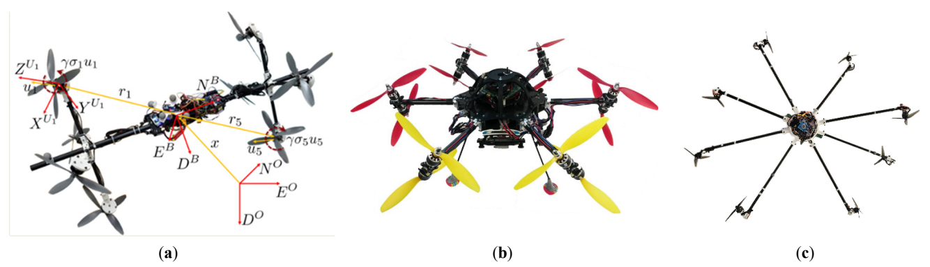
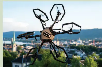
Fixed inclination configuration means that the orientation of a single rotor is fixed with respect to the airframe, and different driving capabilities can be realized by designing the positions and orientations of different rotors during the design process. In actual flight, the total thrust direction can only be adjusted by changing the rotational speed configuration of different rotors. Typical configurations include the eight bi-directional rotor Omni-directional Aerial Robot (ODAR) designed by Park et al. [9], the six-tilt-arm 12-rotor UAV designed by Allenspach et al. [10], and the omni-directional eight-rotor UAV (OmniOcta) designed by Hamandi et al. [11], as shown in Figure 1.
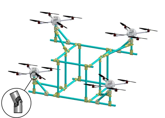
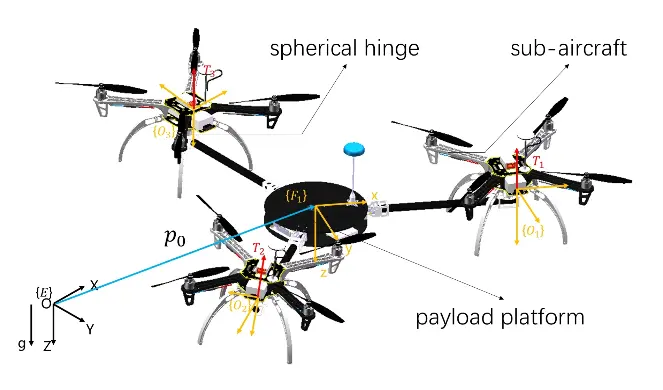
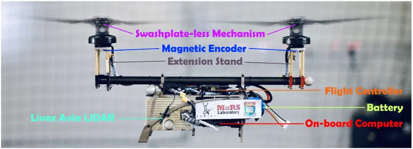
The passive inclination type, i.e., the platform is unable to actively change the direction of rotor thrust, but rather changes the direction of thrust relative to the airframe by means of passive joints (including gimbals and ball joints), is usually constructed by using several quadrotor modules spliced onto the airframe [12,13]. There is also the servo-free dual-rotor unmanned Gemini II proposed by Qin et al. [14] in 2022. These configurations are shown in Figure 2.
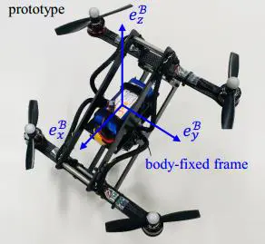
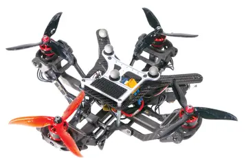
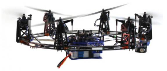
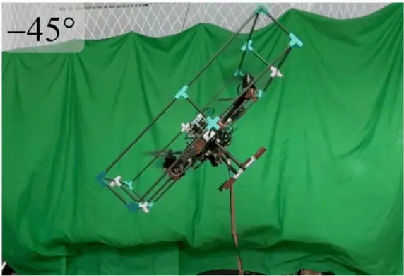
Active inclination thrust-vectoring UAVs offer greater flexibility and have the most research associated with them due to the use of actuators (usually servos) to actively change the direction of thrust. Further, according to whether the change of thrust direction of different rotors is associated or not, they can be further classified into synchronized inclination type and non-synchronized inclination type. The synchronized inclination type usually achieves simultaneous changes in thrust direction across all rotors via parallel mechanical structures or controllers, i.e., the thrust directions of different rotors are correlated. Typical configurations include the parallel-link tilt-quadrotor designed by Sakaguchi et al. [15], the dual-axis tilt-quadrotor TiltDrone designed by Zheng et al. [16], and FAST-Hex designed by Ryll et al. [17]. Non-synchronized inclination type, i.e., the thrust direction of multiple rotors can be changed independently with a greater degree of freedom of control, including Voliro [18], the three-axis tilt-rotor flight platform proposed by Cuniato et al. [19], and Quad3DV [20]. These configurations are shown in Figure 3.
Existing trajectory generation methods mainly focus on coplanar underactuated UAVs, particularly quadrotors. Representative open-source frameworks include Ego-planner [21] and Fast-planner [22], which have been widely used in applications such as agile flight [23], narrow-space traversal [24], and exploration in unknown environments [25]. However, unlike conventional quadrotors that generate 4D trajectories, thrust-vectoring UAVs possess additional actuation degrees of freedom, requiring the simultaneous planning of vehicle states and actuator configurations. Several studies have explored trajectory generation for thrust-vectoring or over-actuated aerial vehicles. For example, Liu et al. [26,27,28] proposed trajectory generation approaches based on quaternion parameterization and polynomial optimization, combined with safe corridor generation and stereographic projection techniques for 6-DoF trajectory construction. Hamandi et al. [29] introduced trajectory optimization with control input smoothing to improve tracking performance, while Hachem et al. [30] employed a direct multiple shooting formulation to enhance maneuverability for fully actuated aerial vehicles. Su et al. [31] proposed a VKC-based motion planning framework for over-actuated UAV systems and later extended the approach using a two-step quadratic programming formulation [32]. Other studies focused on specialized applications, including mixed-reality trajectory generation [33], minimum-time trajectory optimization for articulated thrusters [34], and trajectory planning in confined spaces for tilting bi-rotor UAVs [5]. These works demonstrate the growing interest in trajectory planning for thrust-vectoring aerial vehicles. In addition to motion planning for aerial robots, UAV trajectory optimization has also been widely studied in communication and data collection systems. For example, Liu et al. [35] investigated UAV trajectory optimization for time-constrained environmental monitoring and formulated the problem by considering both Age of Information (AoI) and onboard energy constraints. They decomposed the problem into velocity and path optimization subproblems and proposed an AoI-and-energy-aware trajectory optimization algorithm that combines successive convex approximation (SCA) with a genetic algorithm (GA). Memos et al. [36] proposed an optimized UAV-based data collection strategy for mobile wireless sensor networks (MWSNs). Furthermore, Cui et al. [37] modeled UAV trajectory planning as a Markov decision process (MDP) in scenarios where sensor locations and data volumes are unknown, and developed two model-free trajectory optimization algorithms based on SARSA and Q-learning. These studies demonstrate the broad applicability of UAV trajectory optimization across different application domains.
Although several trajectory generation methods have been proposed for thrust-vectoring or over-actuated UAVs, most existing work focuses on full trajectory optimization without explicitly accounting for constrained corridor environments or the coupled influence of vehicle dynamics and spatial safety margins. In addition, current studies usually rely on conventional quadratic objective functions and lack a systematic evaluation framework for trajectory quality under constrained spaces. As a result, generating dynamically feasible trajectories for thrust-vectoring UAVs while simultaneously considering safety, stability, and efficiency in constrained environments remains insufficiently addressed. Based on this, the main contributions of this paper are as follows: (1) A trajectory generation framework for UAVs operating in pipe-shaped constrained environments; (2) A multi-objective optimization method for generating thrust-vectoring aircraft trajectories is proposed, applicable to both thrust-vectoring aircraft and conventional quadrotors; (3) It establishes a systematic trajectory generation evaluation metric. By comparing it with conventional quadratic objective functions, this study demonstrates the superiority of this multi-objective trajectory generation method. Furthermore, by comparing it with quadrotor flight performance, this method illustrates how it leverages the motion-decoupling advantages of thrust-vectoring aircraft.
The remainder of this paper is organized as follows: Section 2 presents the proposed trajectory generation framework for thrust-vectoring UAVs in pipe-shaped constrained spaces, including the problem formulation, thrust-vectoring UAV modeling, spatial constraint modeling, and the multi-objective optimized trajectory generation method. Section 3 describes the simulation conditions and evaluation metrics, followed by trajectory-generation results for the thrust-vectoring aircraft and comparisons with conventional quadcopter UAVs. Section 4 discusses the characteristics and implications of the proposed trajectory generation method. Finally, Section 5 concludes the paper.
2. Method
2.1. Problem Formulation
It is assumed that the world coordinate system is defined according to the Northeast sky, and the body coordinate system of the UAV is $$x$$-axis facing forward, $$y$$-facing left, as well as $$z$$-facing up. In this paper, the problem of trajectory generation and maneuver planning for a rotorcraft UAV is studied in the $$XOZ$$ plane. Due to the pipe-shaped constrained environment, the lateral motion of the UAV is significantly restricted by the surrounding walls. As a result, the vehicle’s dominant motion occurs primarily in the longitudinal plane of the pipe. Therefore, modeling the UAV motion in the XOZ plane captures the primary translational and attitude dynamics relevant to trajectory generation in such environments, while significantly reducing the complexity of the optimization problem. The trajectory generation problem is formulated as a constrained optimization problem over a finite prediction horizon:
|
```latex\begin{array}{cc}\underset{U}{\text{min}}& J\left(U\right)=\sum\limits _{i=1}^{n}{\alpha }_{i}{L}_{i}+{L}_{terminal}\\ s.t.& {X}_{k+1}=f\left({X}_{k},{U}_{k}\right)\\ & g\left(env,{X}_{k},{U}_{k},params\right)\le 0\\ & {U}_{min}\le {U}_{k}\le {U}_{max}\\ & {X}_{min}\le {X}_{k}\le {X}_{max}\end{array}``` |
(1) |
where $$U=\left\{{u}_{0},{u}_{1},\dots ,{u}_{p-1}\right\}$$ denotes the sequence of control inputs to be optimized over the prediction horizon $$p$$. The UAV state at step $$k$$ is defined as $$X_k=[x_k,z_k,\theta_k,\dot{x}_k,\dot{z}_k,\dot{\theta}_k]^T$$, where $${x}_{k}$$ and $${z}_{k}$$ represent the UAV position in the horizontal and vertical directions, respectively. $${\theta }_{k}$$ denotes the pitch angle, and $${\dot{x}}_{k}$$, $${\dot{z}}_{k}$$ and $${\dot{\theta }}_{k}$$ represent the corresponding velocities. The control input at step $$k$$ is defined as $$U_{k}=[F_{1,k},F_{2,k},\beta_{1,k},\beta_{2,k}]^{T}$$, where $${F}_{1,k}$$ and $${F}_{2,k}$$ denote the thrust generated by the front and rear rotors, respectively, and $${\beta }_{1,k}$$ and $${\beta }_{2,k}$$ denote the corresponding servo tilting angles. For a conventional quadrotor configuration, only the thrust inputs are considered, resulting in two control inputs. The variable $$p$$ denotes the prediction horizon. $${L}_{i}$$ represents the $$i$$-th process cost with the corresponding weight $${\alpha }_{i}$$, and $${L}_{terminal}$$ denotes the terminal cost:
|
```latex{L}_{terminal}=\left({X}_{end}-{X}_{ref}\right){Q}_{t}{\left({X}_{end}-{X}_{ref}\right)}^{T}``` |
(2) |
where $${X}_{end}$$ represents the terminal state of the generated trajectory and $${X}_{ref}$$ represents the desired terminal state.
The process cost consists of four parts: the first part combines the optimization of safety and path length by minimizing the difference from the ideal path, the second part minimizes the time consumption by minimizing the distance to the end point at each step, and the third part reduces the attitude variation by minimizing the attitude angle at each step, which will be presented in 2.4 Multi-Objective Trajectory Generation.
The constraints that need to be satisfied include the dynamics constraints of the UAV itself $$\dot{x}=f\left(x,u\right)$$, the collision-free constraints with the environment $$g\left(env,x,u,params\right)\le 0$$, the control input constraints $${U}_{min} \le U\le {U}_{max}$$, and the state constraints $${X}_{min} \le X\le {X}_{max}$$. The collision-free constraints are modeled as a function of the constraints on the spatial environment $$env$$, the state $$x$$, the control inputs $$u$$, and other parameters $$params$$. The dynamics model is presented in Section 2.2. Thrust-vectoring UAV Modeling, and the characterization of the constrained spatial environment and the construction of collision constraints are presented in Section 2.3. Spatial Constraint Modeling. After this optimization problem is constructed, it is solved using the SQP (Sequential Quadratic Programming) algorithm.
2.2. Thrust-Vectoring UAV Modeling
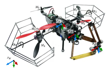
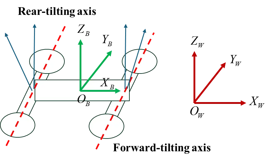
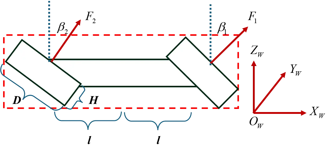
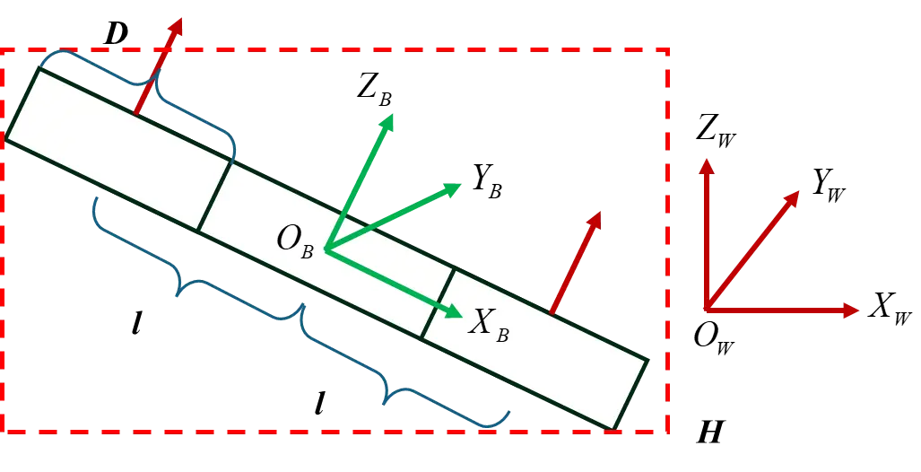
The tilt-tilt quadrotor thrust-vectoring UAV used in this paper is shown in Figure 4, and its structure is similar to the platform proposed by Shu et al. [3]. The front two rotors are fixed on an arm that can tilt around the $$Y$$-axis of the fuselage at an angle that conforms to the right-hand rule, and similarly, the rear two rotors are fixed on a rotating arm. The four rotors are positioned at the four vertices of a square, and at the same time, the four rotors have identical characteristics. Therefore, when the two rotors on the left and right sides of each arm have the same rotational speed, the whole airplane can be simplified to a planar forward flight model as in Figure 5a, while the conventional four-rotor Figure 5b can be regarded as a special case of it (with both rudders swinging at $$0°$$).
 |
 |
|
(a) |
(b) |
Figure 5. Simplified model in forward flight. (a) Tilt-rotor quadcopter. (b) Conventional quadcopter.
When simplified to a planar model, the whole system at this point is a 4-input, 3-output system with the following dynamics model:
|
```latex\begin{cases} \ddot{x} = \dfrac{F_{1}\sin(\beta_{1}+\theta)+F_{2}\sin(\beta_{2}+\theta)}{m} \\ \ddot{z} = \dfrac{F_{1}\cos(\beta_{1}+\theta)+F_{2}\cos(\beta_{2}+\theta)}{m} - g \\ \ddot{\theta} = \dfrac{-F_{1}l\cos\beta_{1}+F_{2}l\cos\beta_{2}}{I_{\mathrm{YY}}} \end{cases}``` |
(3) |
where $${F}_{1}$$, $${F}_{2}$$, $${\beta }_{1}$$ and $${\beta }_{2}$$ are four inputs, which are the total lift provided by the two rotors on the frontside and backside arms as well as the arm tilting angles of the frontside and backside arms, respectively. $$x$$, $$z$$, and $$\theta$$ are the longitudinal position, the vertical position, and the pitch angle, respectively. $$l$$ is half of the center distance between the front and backside rotors, and the other shape parameters are the envelope diameter of the duct rotor $$D$$ as well as the envelope height $$H$$, which will be used to generate the collision judgment point of the UAV. $$m$$ is the mass of the whole aircraft, $$g$$ is the gravitational acceleration, and $${I}_{YY}$$ is the rotational inertia around the $$Y$$-axis.
For a single rotor blade, the following model is used to describe it:
|
```latex\begin{cases} F = k_{T}N^{2} \\ M = k_{M}N^{2} \\ P = MN/9.55 \end{cases}``` |
(4) |
where $$F$$ is the rotor lift, $$M$$ is the rotor torque, $$P$$ is the rotor power, $$N$$ is the rotor rotational speed, and $${k}_{T}$$ and $${k}_{M}$$ are the integrated lift coefficient and integrated torque coefficient of the rotor, respectively.
Before constructing the collision inequality constraints under the pipeline boundary constraints, it is necessary to set the collision determination rules for the UAV. In this paper, the UAV is constructed as a 3 rectangular rigid body, then its 12 vertices are used as the set of judgment collision points. $${\mathcal{P}}_{UAV}$$, which is the mapping of states as well as inputs. For a quadrotor UAV, it can be simplified as a rectangle of length $$\left(2l+D\right)$$ and height $$H$$. The rectangle can be used to determine the collisions of the UAV.
|
```latex{\mathcal{P}}_{UAV}=\left\{{p}_{UAV}^{\left(i\right)}\left(x,z,\theta ,{\beta }_{1},{\beta }_{2}\right)\in {\mathbb{R}}^{2}\mid i=1,\dots ,12\right\}``` |
(5) |
2.3. Spatial Constraint Modeling
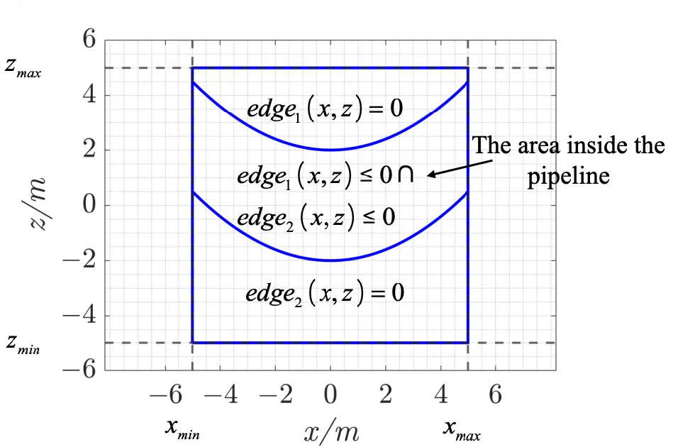
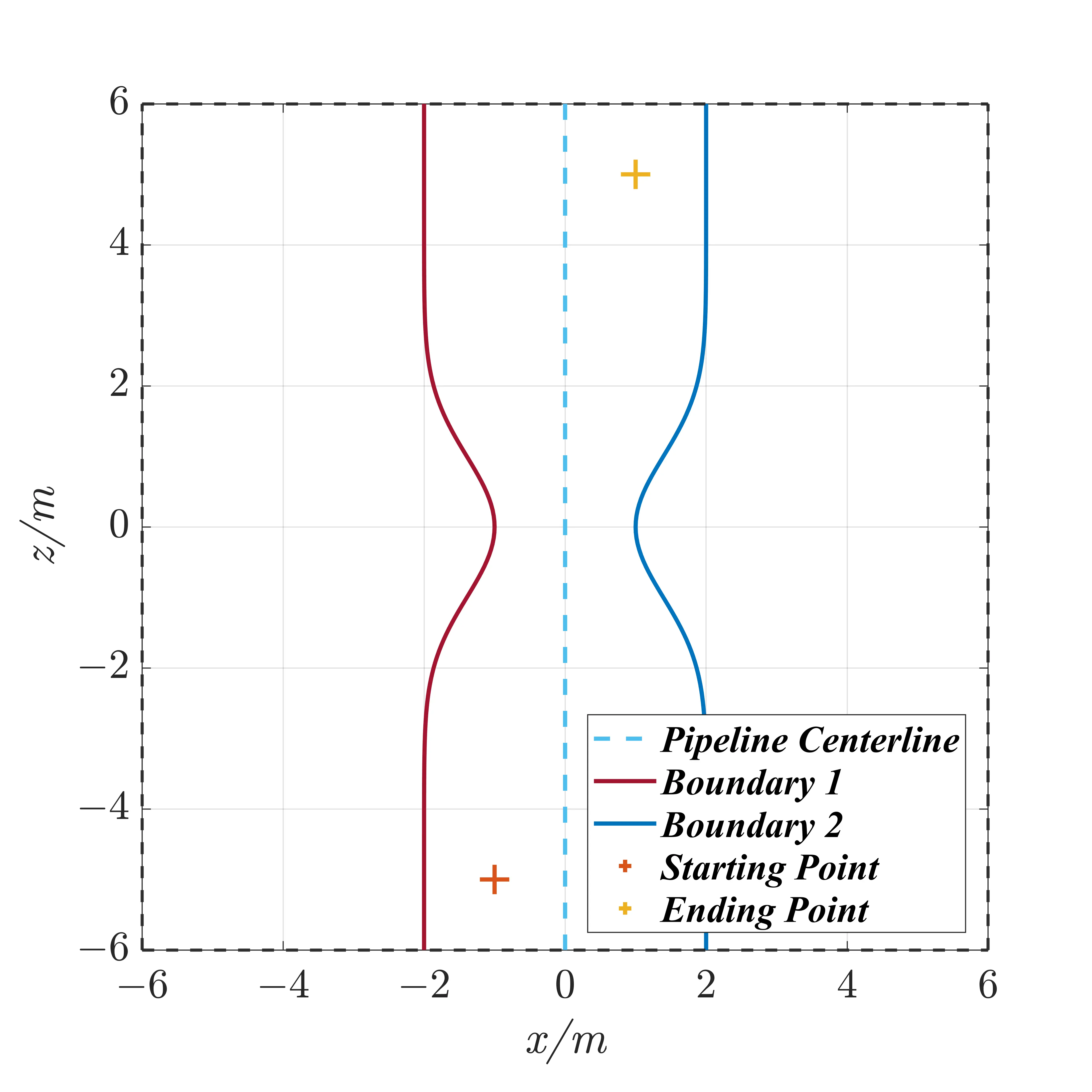
In this paper, the constraint space is defined as a region surrounded by bounding rectangles and curves, and a typical pipeline constraint space is shown in Figure 6, which contains the range boundaries of the coordinates as well as the shape boundaries of the pipeline, and can be defined in the following mathematical form:
|
```latexenv = \{(x,z) \mid x_{\min} \leq x \leq x_{\max}, z_{\min} \leq z \leq z_{\max}, \forall i \in \{1,\dots,n\}, edge_i(x,z) \leq 0\}``` |
(6) |
where $$env$$ denotes the set of points in the feasible region of the constraint space, which needs to satisfy the range constraints of the coordinates as well as the boundary judgment conditions. $$edg{e}_{i}\left(x,z\right)=0$$ denotes the curve equation corresponding to the boundary $$i$$ of the pipeline. The uniform definition of $$edg{e}_{i}\left(x,z\right)\le 0$$ indicates that within this boundary, it is a feasible region. $$n$$ denotes the number of boundaries, and to simplify the problem and without loss of generality, this paper studies the case of the case of $$n=2$$ is studied.
After defining the environmental parameters $$env$$ and the vertex coordinate set of the UAV $${\mathcal{P}}_{UAV}$$, the inequality constraint of the corridor boundary under a given safety distance $${d}_{safe}$$ can be expressed as follows:
|
```latex\forall {p}_{i}\in {\mathcal{P}}_{UAV},j\in \left\{1,\dots ,n\right\},-d\left({p}_{i},edg{e}_{j}\right)+{d}_{safe}\le 0``` |
(7) |
where $$d\left({p}_{i},edg{e}_{j}\right)$$ represents the minimum distance from the point $${p}_{i}$$ to the boundary $$edg{e}_{j}\left(x,z\right)=0$$. The boundary curve is discretized into $${N}_{j}$$ points $${\mathcal{E}}_{j}$$, and the minimum distance between $${p}_{i}$$ and these points are computed as follows:
|
```latexd\left({p}_{i},edg{e}_{j}\right)=\underset{q\in {\mathcal{E}}_{j}}{\mathrm{min}}\parallel {p}_{i}-q{\parallel }_{2},where\, {\mathcal{E}}_{j}=\left\{\left({x}_{k},{z}_{k}\right)\in {\mathbb{R}}^{2}\mid edg{e}_{j}\left({x}_{k},{z}_{k}\right)=0,k=1,\dots ,{N}_{j}\right\}``` |
(8) |
2.4. Multi-Objective Optimized Trajectory Generation
During the trajectory generation process, it is necessary to comprehensively consider factors such as trajectory safety, stability, and rapidity. Based on the optimization framework established in Section 1, this section provides a detailed introduction to the trajectory cost function. First, the first part of the cost function is defined as the deviation between the generated and reference trajectories, using the multi-edge wheel distance evaluation method in PoLis [1]. The deviation between two trajectories is defined by the following metric:
|
```latex{L}_{1}=D\left(T,R\right)=\frac{1}{2q}\sum\limits _{i=1}^{q}\underset{\mathbf{r}\in \mathcal{R}}{\text{min}}\parallel {\mathbf{e}}_{i}-\mathbf{r}{\parallel }_{2}+\frac{1}{2r}\sum\limits _{j=1}^{r}\underset{\mathbf{e}\in \mathcal{E}}{\text{min}}\parallel {\mathbf{r}}_{j}-\mathbf{e}{\parallel }_{2}``` |
(9) |
The symbols used in the formula are defined as follows: $${\mathbf{e}}_{i}\in {\mathbb{R}}^{2}$$ denotes the $$i$$-th sampled point on the generated trajectory, belonging to the set of generated trajectory points $$T$$; $${\mathbf{r}}_{j}\in {\mathbb{R}}^{2}$$ denotes the $$j$$-th sampled point on the reference trajectory, belonging to the reference trajectory point set $$R$$; $$q$$ and $$r$$ are the numbers of points in the generated and reference trajectories, respectively, i.e., $$\left|T\right|=q$$, $$\left|R\right|=r$$; $$\parallel \cdot {\parallel }_{2}$$ denotes the Euclidean norm, representing the distance between two points. Ideally, the trajectory should be located at the centerline of the corridor boundary and should move synchronously within the corridor during trajectory generation. The corridor curve defined in this paper is symmetric and parallel to the central axis, where the central axis is defined as the trajectory obtained by translating or scaling the symmetric curve by half of the corridor width. Since the distance between the central axis points and the corridor boundary is usually the largest, this metric is used to evaluate the safety of the generated trajectory.
The second part of the cost function minimizes the deviation between the predicted terminal position and the target position at each prediction step, so as to guide the vehicle to reach the target state more quickly. This term takes the form of a standard quadratic function, and its expression is as follows:
|
```latex{L}_{2}=\sum\limits _{i=1}^{p}{\left({\mathbf{x}}_{\mathbf{i}}-\mathbf{r}\right)}^{T}{Q}_{p}\left({\mathbf{x}}_{\mathbf{i}}-\mathbf{r}\right)``` |
(10) |
The third part of the cost function minimizes the control effort, aiming to reduce energy consumption and thus achieve the goal of energy efficiency. Its expression is as follows:
|
```latex{L}_{3}=\sum _{i=1}^{p}{u}^{T}{R}_{p}u``` |
(11) |
The fourth part of the cost function is the average pitch angle of the planned trajectory, penalizing excessive attitude changes during motion. Its expression is as follows:
|
```latex{L}_{4}=\frac{1}{p}\sum _{i=1}^{p}{\theta }_{i}``` |
(12) |
where $${\theta }_{i}$$ denotes the pitch angle at each prediction step.
The cost function is designed to balance multiple objectives involved in UAV motion within pipe-shaped constrained environments. Specifically, the trajectory smoothness terms are introduced to ensure dynamically feasible and smooth motion, while the control-related terms are used to limit excessive actuator maneuvers and improve tracking stability. In addition, distance-related terms are incorporated to maintain safe clearance from obstacles and the pipe boundary. These objectives jointly reflect the key requirements of trajectory generation in constrained environments, including safety, smoothness, and maneuverability.
The resulting trajectory generation problem is nonlinear and nonconvex due to the UAV dynamics and obstacle-avoidance constraints. In this work, a sequential quadratic programming (SQP) solver is adopted to handle the nonlinear constrained optimization problem. To improve convergence reliability, the optimization is initialized using the centerline of the pipe-shaped corridor, which provides a feasible initial trajectory. In the tested scenarios, the solver consistently converges to feasible solutions without numerical instability. In addition, the spatial constraint formulation is based on smooth geometric representations, ensuring that the distance function remains continuous and avoiding severe discontinuities during optimization.
3. Results
3.1. Simulation Conditions and Evaluation Metrics
The trajectory optimization simulations were implemented in MATLAB, and the nonlinear constrained optimization problem was solved using the Sequential Quadratic Programming (SQP) algorithm. The sampling time is $${T}_{s}=0.1$$ s, and both the prediction horizon and control horizon are set to 50 steps. The main parameters of the thrust-vectoring aircraft used in this study are shown in Table 1.
Table 1. Main parameters of the thrust-vectoring aircraft.
|
Parameter |
Symbol |
Value |
|---|---|---|
|
Total mass of aircraft |
$$m$$ |
$$2.5\, \mathrm{k}\mathrm{g}$$ |
|
Gravitational acceleration |
$$g$$ |
$$9.8\, \mathrm{m}/{\mathrm{s}}^{2}$$ |
|
Maximum thrust of front/rear rotor |
$${F}_{\mathrm{m}\mathrm{a}\mathrm{x}}$$ |
$$28.5\, \mathrm{N}$$ |
|
Moment of inertia about $$y$$-axis |
$${I}_{yy}$$ |
$$6.7×{10}^{-2} \,\mathrm{k}\mathrm{g}/{\mathrm{m}}^{2}$$ |
|
Half distance between front and rear rotors |
$$l$$ |
$$0.2\, \mathrm{m}$$ |
|
Ducted rotor outer diameter |
$$D$$ |
$$0.2\, \mathrm{m}$$ |
|
Ducted rotor height |
$$H$$ |
$$0.05 \,\mathrm{m}$$ |
|
Thrust coefficient |
$${k}_{T}$$ |
$$1.23×{10}^{-7} \,\mathrm{N}/\mathrm{r}\mathrm{p}{\mathrm{m}}^{2}$$ |
|
Torque coefficient |
$${k}_{M}$$ |
$$2.22×{10}^{-6}\, \mathrm{N}\cdot \mathrm{m}/\mathrm{r}\mathrm{p}{\mathrm{m}}^{2}$$ |
|
Average power of servos (both 2) |
$${P}_{\mathrm{s}\mathrm{e}\mathrm{r}\mathrm{v}\mathrm{o}}$$ |
$$22\, \mathrm{W}$$ |
The main optimization parameters used in the trajectory generation framework are summarized in Table 2. These parameters were selected based on empirical tuning to balance trajectory smoothness, control effort, and obstacle avoidance performance. In all tested scenarios, the optimization solver consistently converged to feasible solutions without numerical instability. The optimization typically converges within several seconds on a standard desktop computer.
Table 2. Main optimization parameters.
|
Parameter |
Description |
Value |
|---|---|---|
|
Optimization solver |
Nonlinear programming solver |
Sequential Quadratic Programming (SQP) |
|
State dimension |
UAV state vector dimension |
6 |
|
Control dimension (quadrotor) |
Number of control inputs |
2 |
|
Control dimension (tilting UAV) |
Number of control inputs |
4 |
|
Prediction state weight matrix ($${Q}_{p}$$) |
State tracking weight during prediction horizon |
$$diag\left(1,1,10,0,0,0\right)$$ |
|
Control weight matrix ($${R}_{p}$$) |
Control effort weight |
$$diag\left(1,1\right)$$ |
|
Terminal state weight ($${Q}_{t}$$) |
Terminal state penalty |
$$diag\left(1,1,1,1,1,1\right)$$ |
|
Terminal control weight ($${R}_{t}$$) |
Terminal control penalty |
$$0$$ |
|
Initial trajectory |
Initial guess for optimization |
pipeline centerline |
|
Optimization type |
Problem formulation |
Nonlinear constrained optimization |
|
Sampling time ($${T}_{s}$$) |
Discrete sampling time |
0.1 s |
|
Prediction horizon ($${N}_{p}$$) |
Prediction steps |
50 |
|
Control horizon ($${N}_{c}$$) |
Control steps |
50 |
|
Simulation time |
Total simulation duration |
5 s |
|
Safety distance ($${d}_{safe}$$) |
Minimum obstacle clearance |
0.4 m |
|
Maximum solver iterations |
Maximum iterations of optimization |
50 |
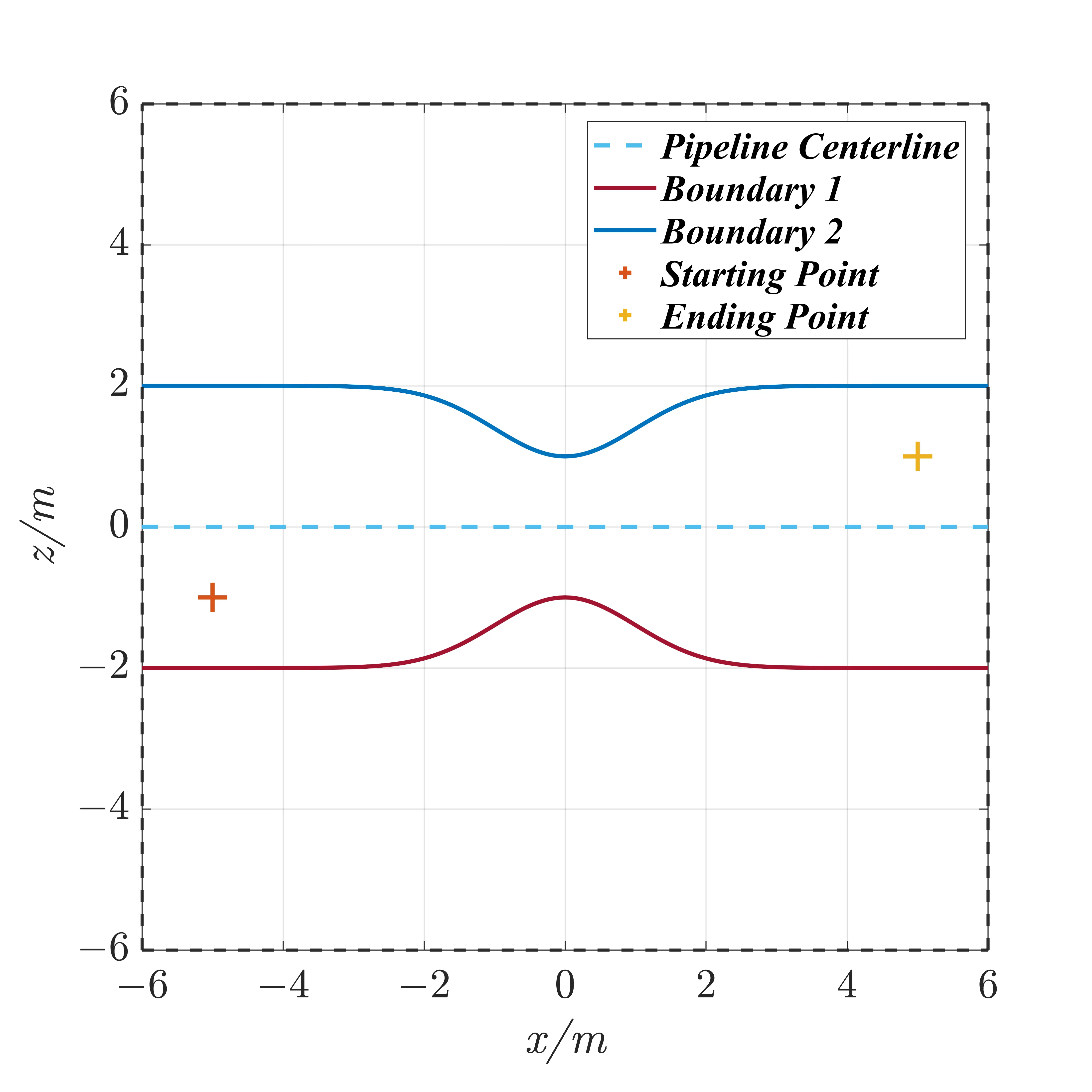
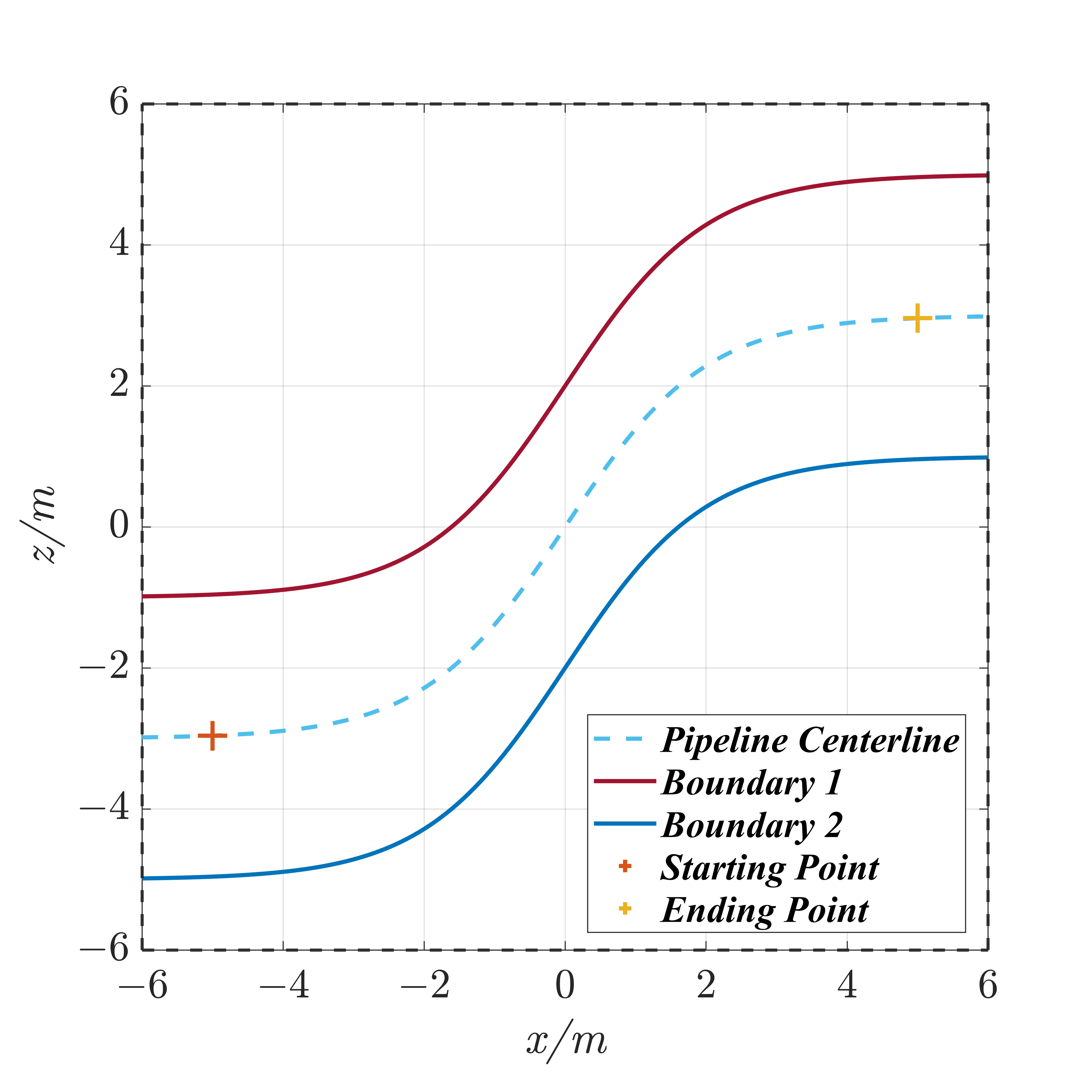
The simulation conditions are set as follows: according to the above configuration, three types of corridor spaces are constructed as shown in Figure 7. The start and end points are specified, and the multi-objective trajectory generation method proposed in this paper is applied. The generated trajectories are used to plan and evaluate the path of the thrust-vectoring aircraft under different spatial constraints.
 |
 |
 |
|
(a) |
(b) |
(c) |
Figure 7. Three typical pipeline scenarios. (a) Horizontal transition radius. (b) Vertical transition radius. (c) S-shaped transition radius.
Referring to the evaluation framework for ground vehicle trajectories proposed by Shu et al. [38], this paper establishes the following metrics to evaluate the generated trajectories:
-
Proximity to the ideal trajectory: This index measures how closely the generated trajectory matches the ideal reference path. The notation is defined as $$D\left(T,R\right)$$, and its calculation method is consistent with the previously defined $${L}_{3}$$.
-
Attitude variation: This term includes the range of pitch angle variation $$\mathrm{\Delta }\theta$$ and the integral average pitch angle $$\bar{\theta }$$, which are calculated as follows:
```latex\begin{aligned}&\Delta\theta=\theta_{max}-\theta_{min}\\&\overline{\theta}=\frac{1}{t}\int_{0}^{t}\lvert\theta\rvert d\tau\end{aligned}```
(13)
where $${\theta }_{max}$$ and $${\theta }_{min}$$ represent the maximum and minimum pitch angles, respectively, and $$t$$ is the total time duration. The comprehensive attitude variation index $${L}_{\theta }$$ is defined as the combination of the two terms, given by:
|
```latexL_\theta=\Delta\theta+\bar{\theta}``` |
(14) |
- 3.
-
Total Energy Consumption: For the thrust-vectoring aircraft, the total energy consumption $$W$$ consists of the energy consumed by the rotors and by the servos. Assuming the servo power remains constant during operation, the instantaneous total power $$P$$ can be expressed as:
```latexP={P}_{rotots1}+{P}_{rotors2}+{P}_{servo}```
(15)
where $${P}_{\text{rotors}\left\{i\right\}}\left(i=1,2\right)$$ denotes the power of the front and rear rotors, respectively. Based on the previously established propulsion system model, the rotor power is calculated as:
|
```latex{P}_{rotors\left\{i\right\}}=\frac{{k}_{M}}{9.55{k}_{T}^{1.5}}{F}^{1.5}, i=1,2``` |
(16) |
The total energy consumption $$W$$ is then given by:
|
```latexW=\frac{1}{t}{\int }_{0}^{t}Pd\tau``` |
(17) |
- 4.
-
Time to Reach Target: The time to reach the target, denoted as $${t}_{reach}$$, is defined as follows to characterize the rapidity of the trajectory:
```latex{t}_{reach}=\mathrm{min}\left\{{t}_{i}\in \left[0,t\right] | \forall {t}_{j}\ge {t}_{i}, D\left({t}_{j}\right)\le {\delta }_{d} \wedge {E}_{\theta }\left({t}_{j}\right)\le {\delta }_{\theta }\right\}```
(18)
where $$D\left(t\right)=\sqrt{{\left(x\left(t\right)-{x}_{d}\right)}^{2}+{\left(z\left(t\right)-{z}_{d}\right)}^{2}}$$ represents the distance between the current position and the target position, $${\delta }_{d}$$ is the predefined position tolerance, and $${E}_{\theta }\left(t\right)=\left|\theta \left(t\right)-{\theta }_{d}\right|$$ denotes the pitch angle error. $${\delta }_{\theta }$$ is the specified pitch angle tolerance.
- 5.
-
Trajectory Safety: Trajectory safety is characterized by the minimum distance $${D}_{min}$$ and the average distance $$\stackrel{‾}{D}$$ between the UAV and the constraint boundaries, defined as follows:
```latexD_{min}=\min D_{i}\left(\mathcal{P}_{UAV},en\nu\right)\\\bar{D}=\frac{1}{p}\sum_{i=1}^{p}D_{i}\left(\mathcal{P}_{UAV},en\nu\right)```
(19)
where $${D}_{i}\left({\mathcal{P}}_{{UAV}},env\right)$$ represents the distance between the UAV and the surrounding environment at the $$i$$-th prediction step. Similar to the definition above, each collision-checking point in the UAV point set $${\mathcal{P}}_{{UAV}}$$ is used to calculate the minimum distance to the environmental boundary. During optimization, the curve distance is discretized into a sequence of points, and the SQP algorithm is used to find the minimum distance between the trajectory point and the implicit surface function representing obstacles. For comparison, a trajectory risk index $${L}_{{risk}}$$ is defined as follows:
|
```latexL_{risk}=\frac{1}{D_{min}}+\frac{1}{\bar{D}}``` |
(20) |
- 6.
-
Radar Chart Area: Finally, the indicators $$D\left(T,R\right)$$, $${L}_{\theta }$$, $$W$$, $${t}_{{reach}}$$, and $${L}_{{risk}}$$ are used to evaluate the stability, economy, rapidity, and safety of the generated trajectories. Since all indicators are designed such that smaller values correspond to better performance, they are normalized for comprehensive comparison. According to these five indicators, a radar chart is plotted, and each indicator is normalized as follows:
```latex\hat{L}_i=\frac{L_i}{L_{i,max}}```
(21)
where $${L}_{i}$$ represents the value of the $$i$$-th indicator under the current condition, and $${L}_{i,max}$$ denotes the maximum value of the indicator among all test cases. For $${t}_{{reach}}$$, if the target condition is not reached during the simulation, the corresponding value is set to half of the total simulation time. After normalization, all indicators fall within the range $$\left[0,\mathrm{ }1\right]$$, and the radar chart is plotted with evenly distributed angles. The total area is computed as a polygon area.
3.2. Trajectory Generation Results of the Thrust-Vectoring Aircraft
To verify the effectiveness of the proposed multi-objective trajectory generation method, a comparison is made with a conventional quadratic objective function. The conventional quadratic cost function includes only the process-related terms $${L}_{2}$$ and $${L}_{3}$$, as well as the terminal cost term, expressed as:
|
```latex{L}^{\prime}={\alpha }_{2}{L}_{2}+{\alpha }_{3}{L}_{3}+{L}_{terminal}``` |
(22) |
Other simulation conditions remain consistent. The generated trajectory diagrams (Figure 8), state change sequences (Figure 9 and Figure 10), input change sequences (Figure 11), evaluation metrics (Table 3), and radar charts (Figure 12) under the aforementioned three operating conditions are shown in the figure below.
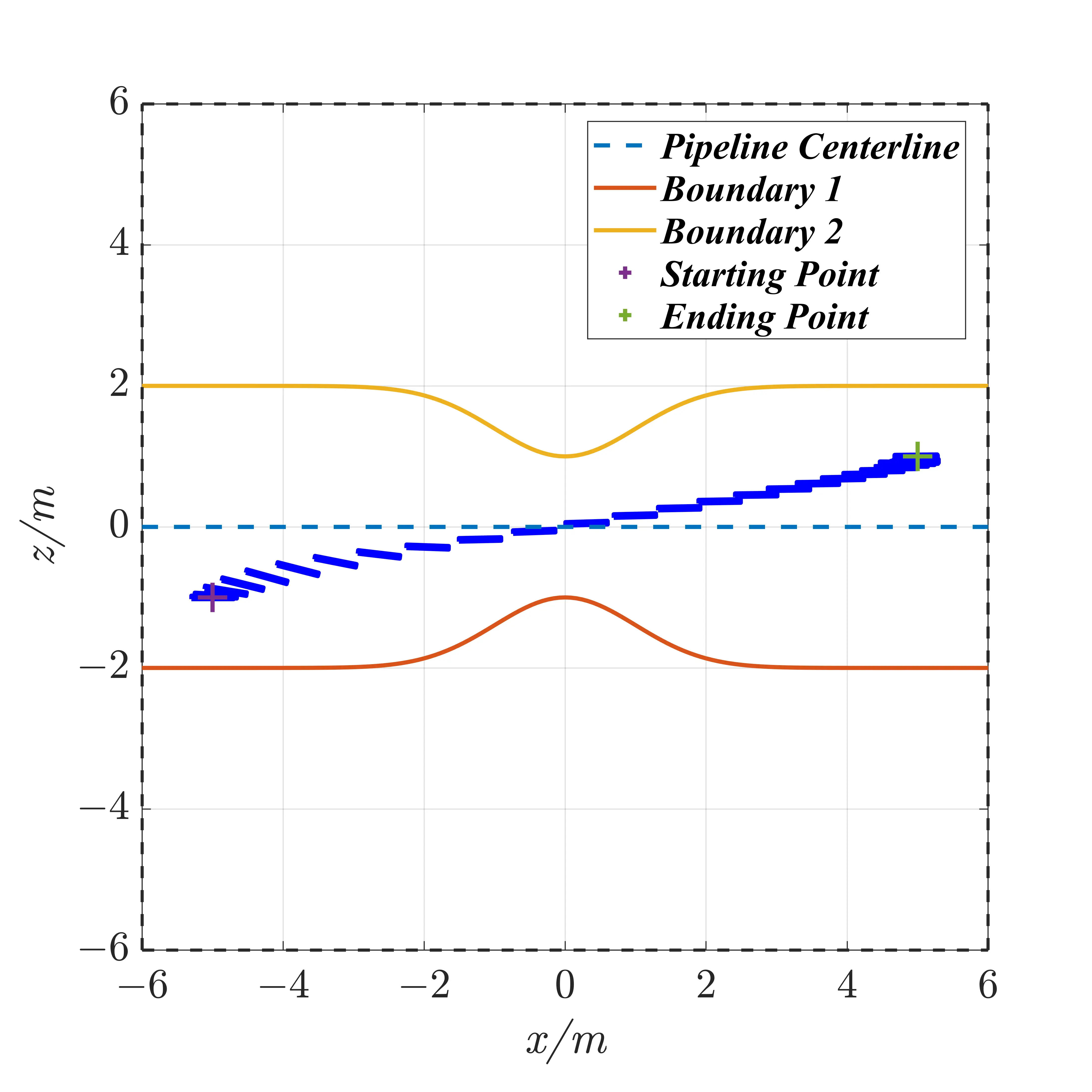
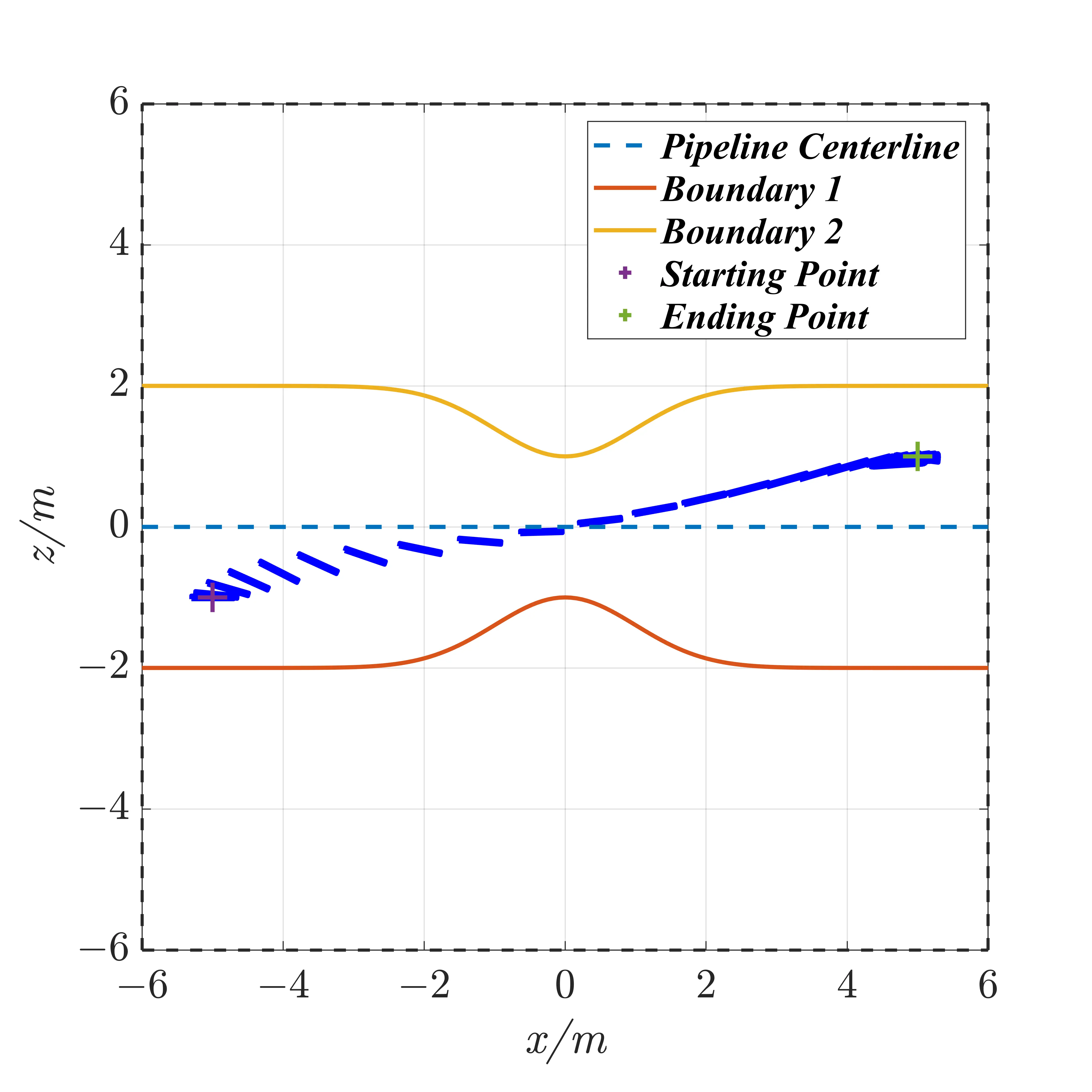
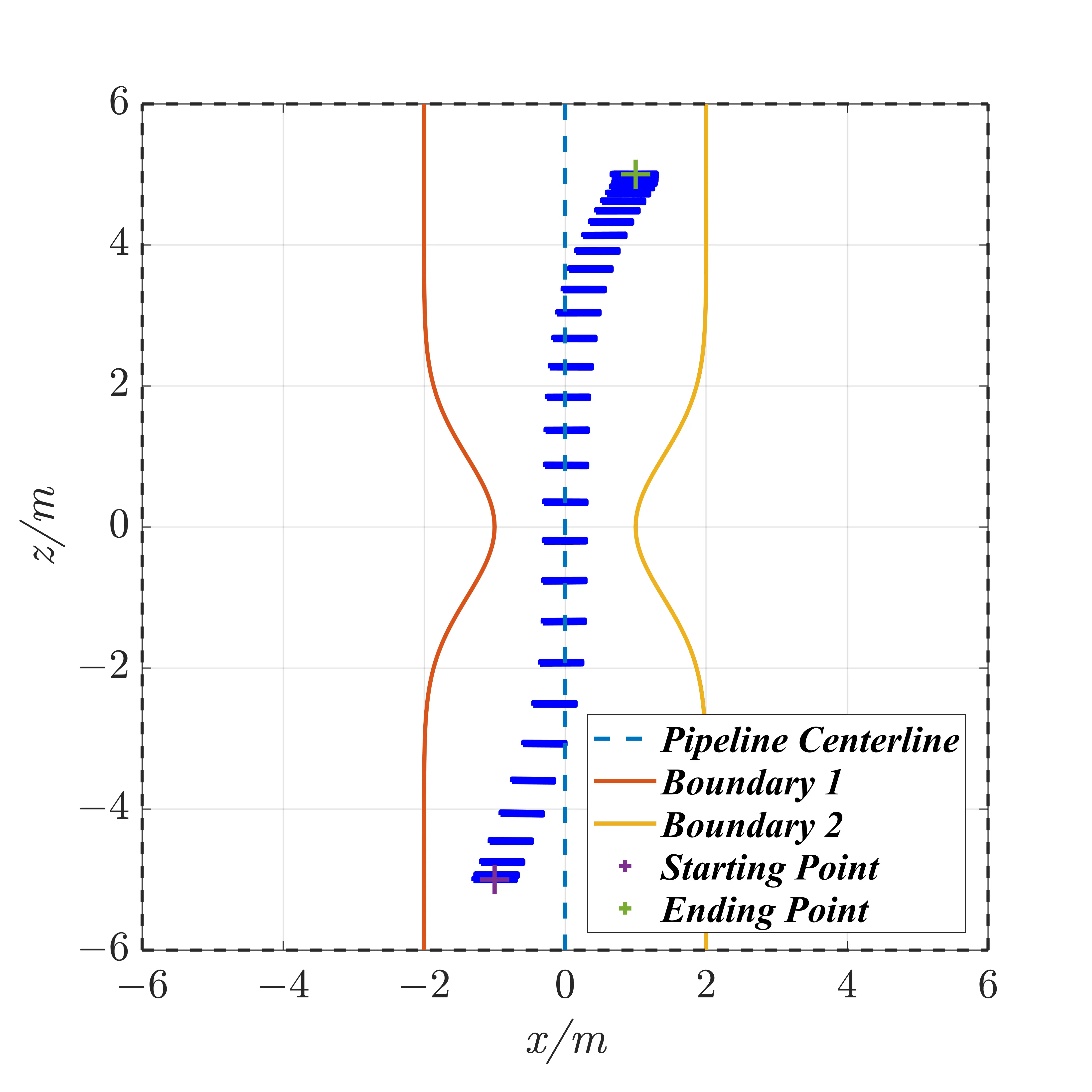
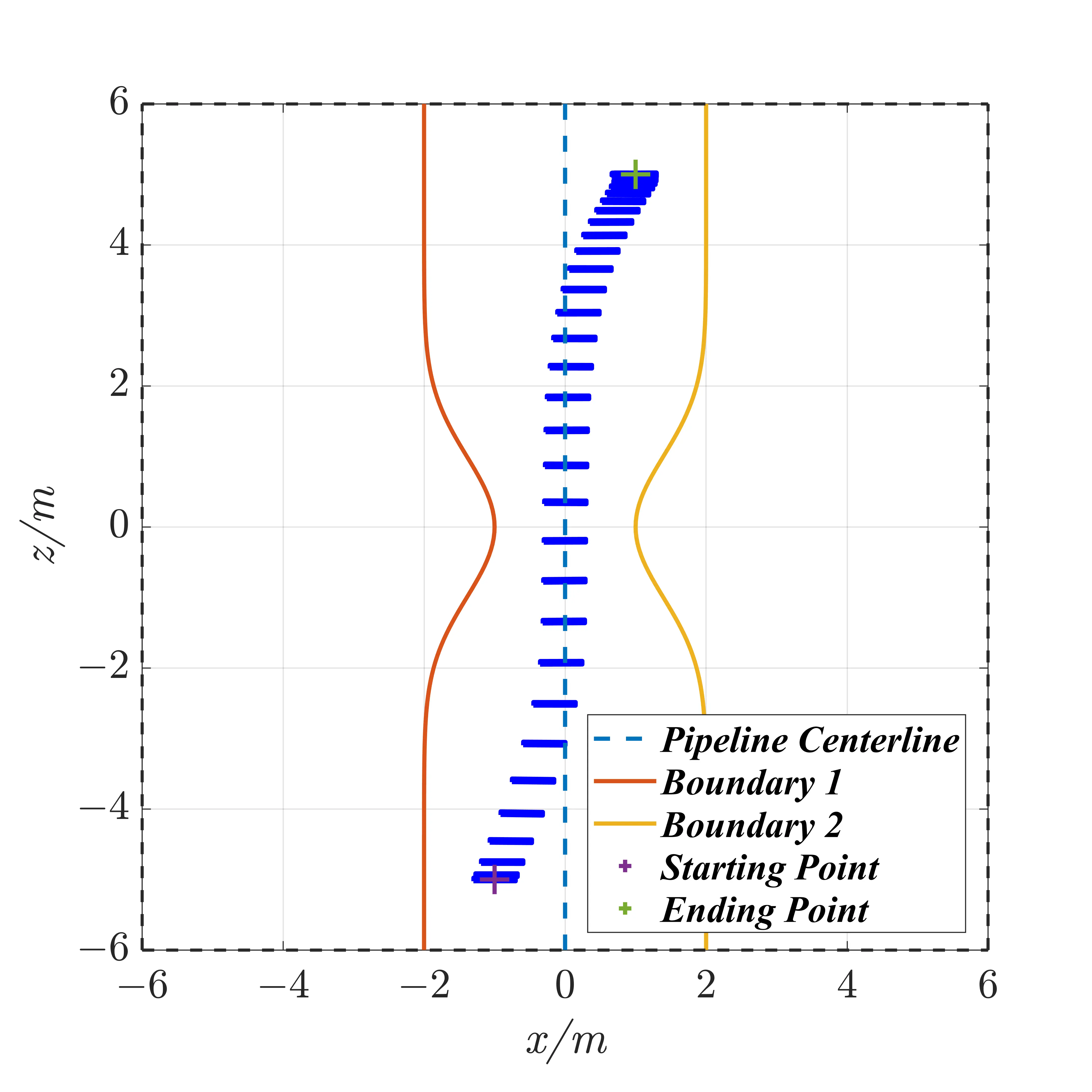
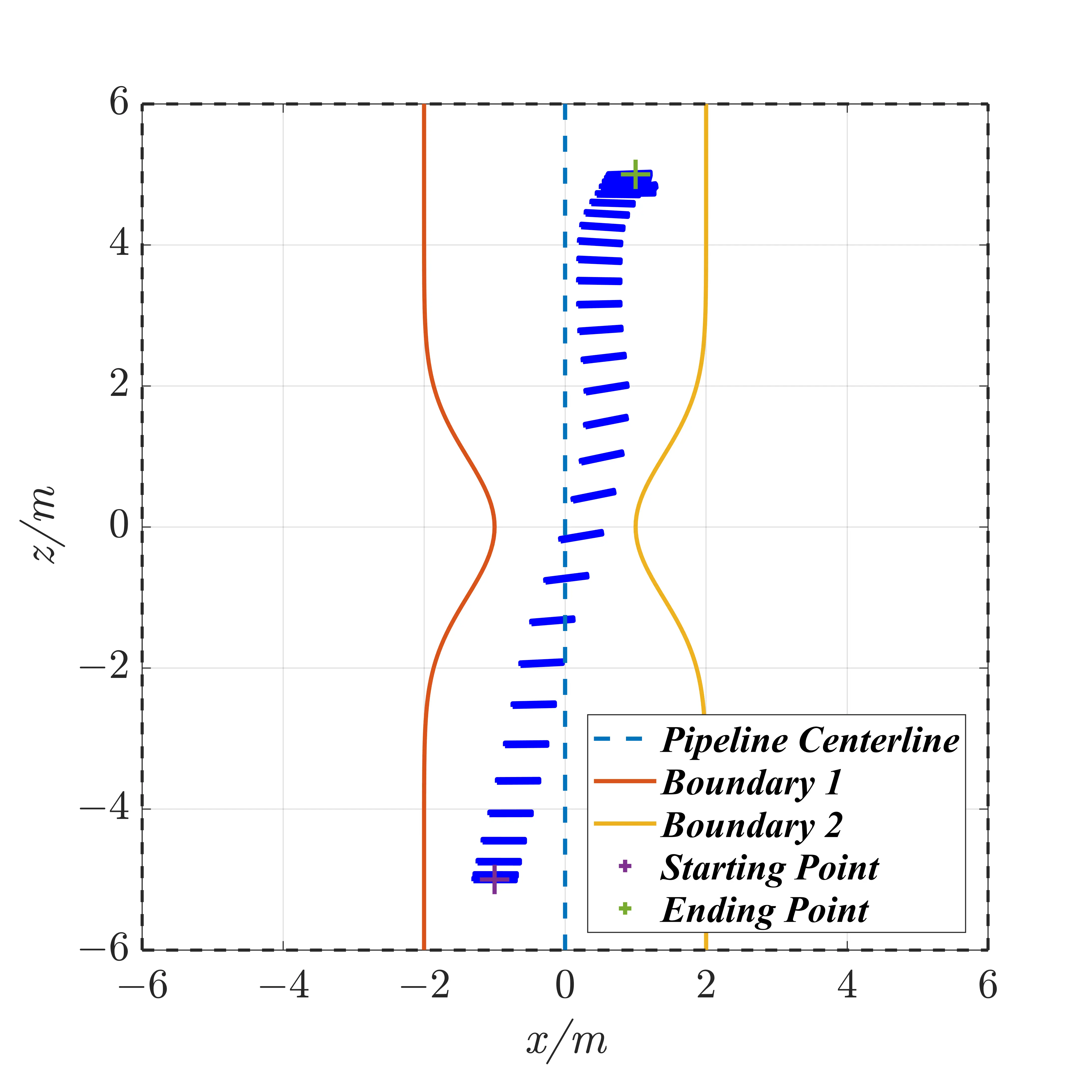
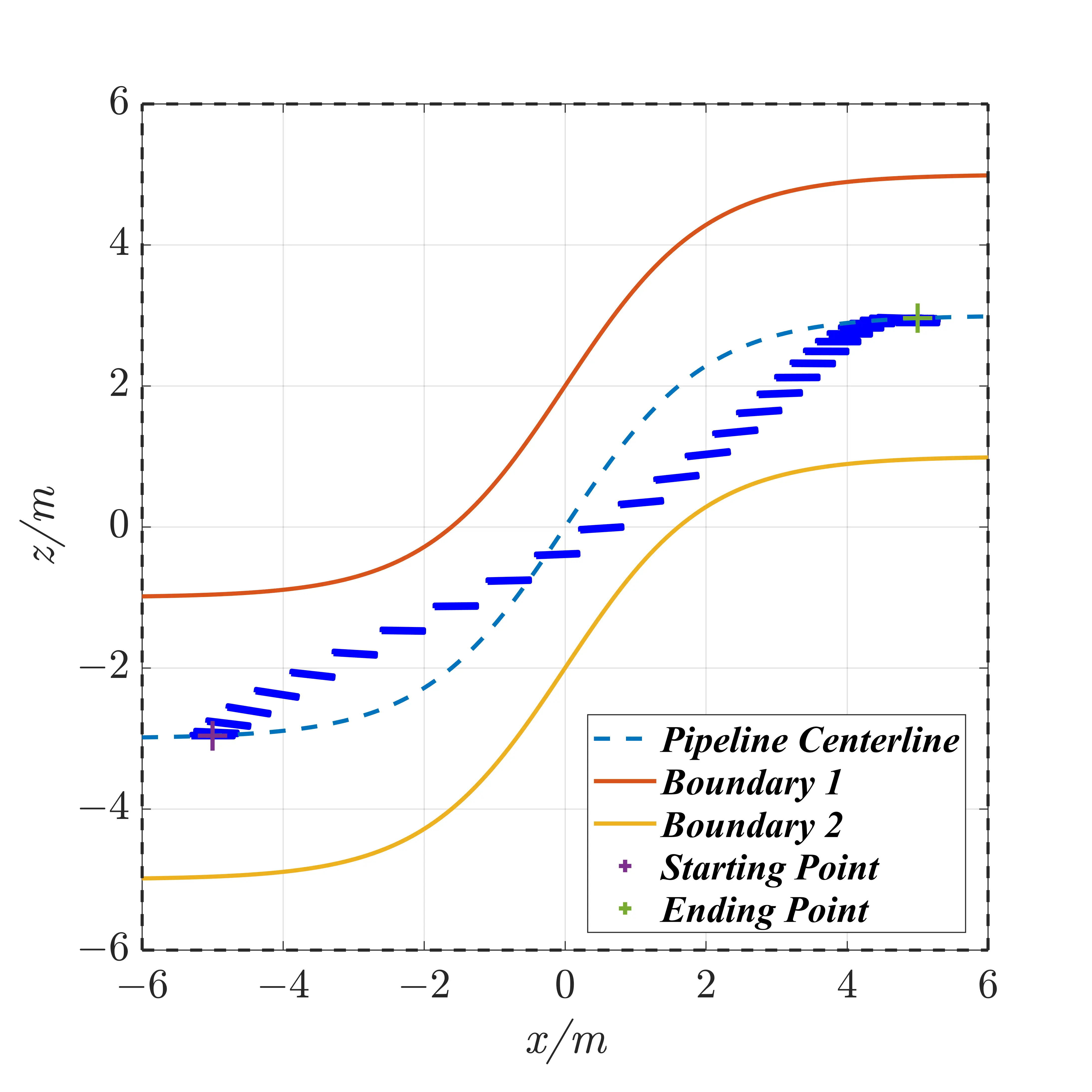
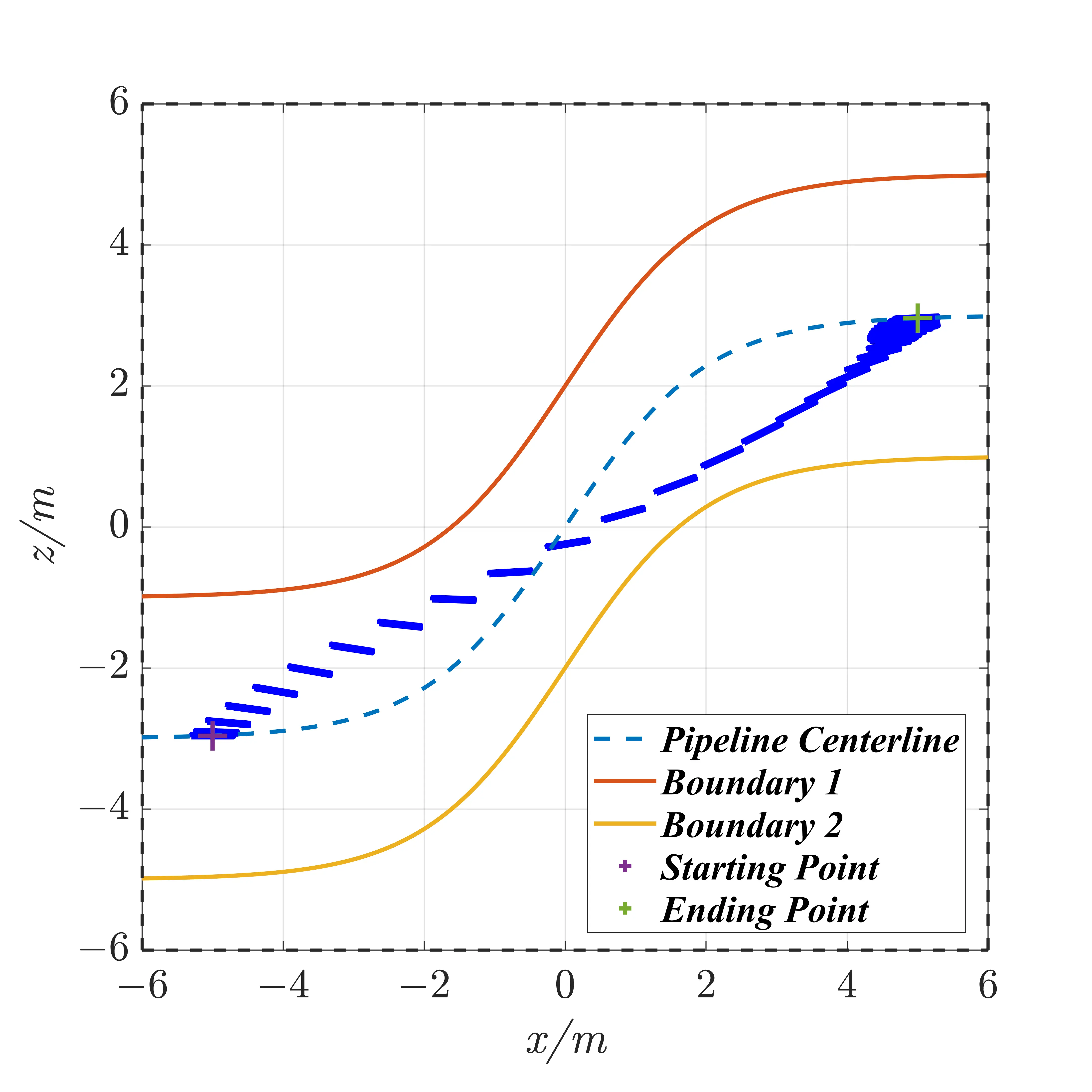
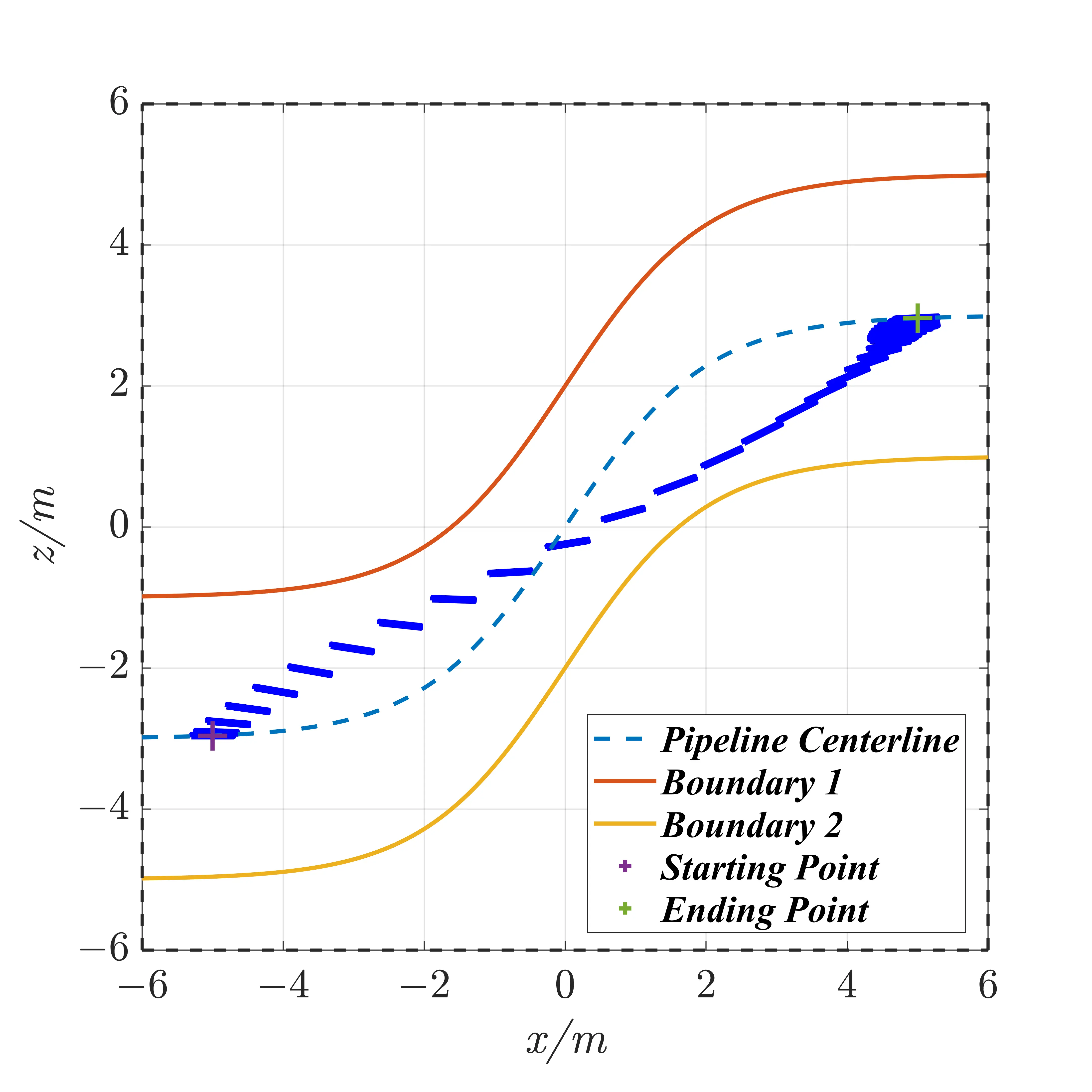
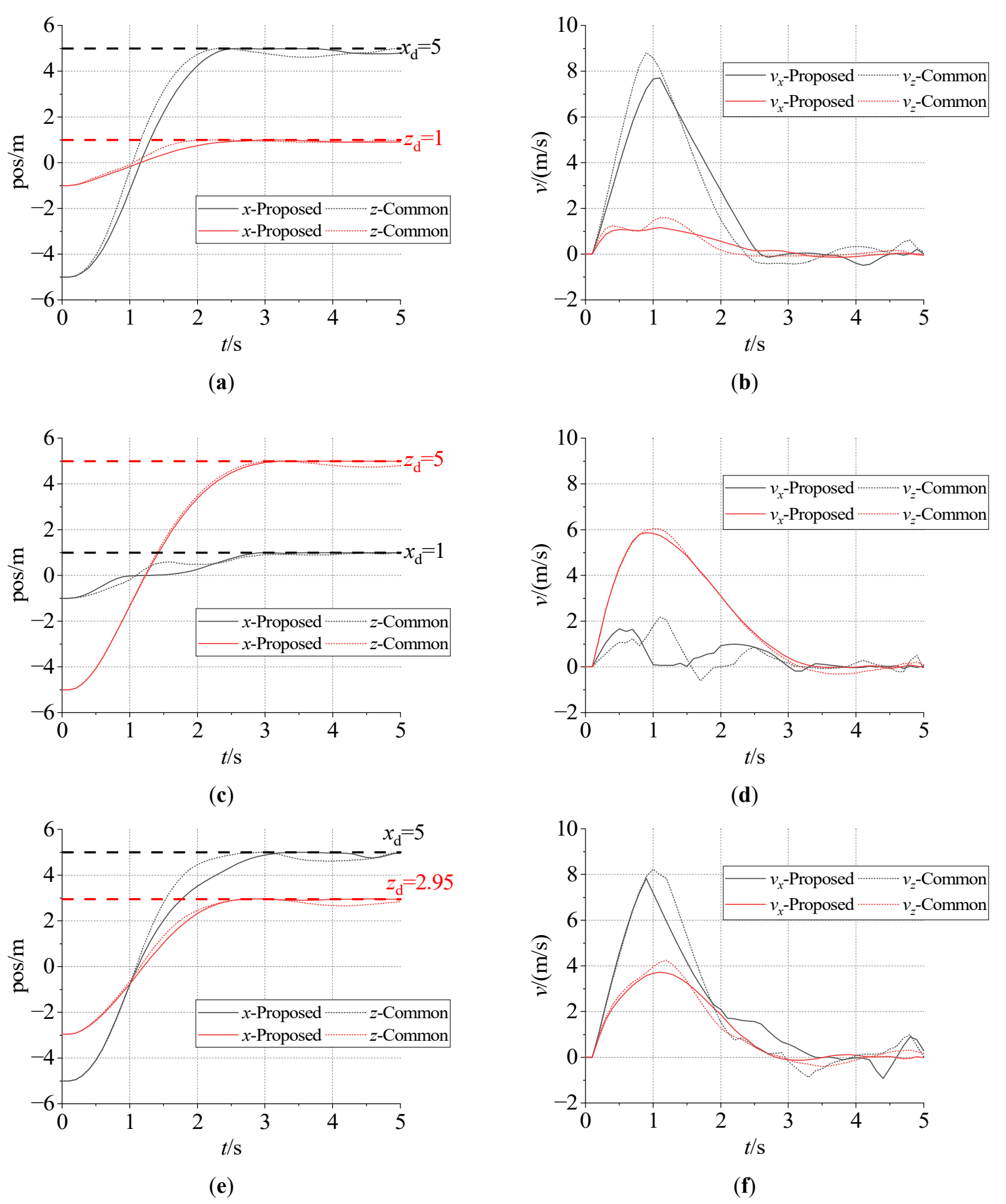
Figure 9. Position and Attitude Planning Results. (a) Position of the transverse pipeline. (b) Velocity of the transverse pipeline. (c) Position of the vertical pipeline. (d) Velocity of the vertical pipeline. (e) Position of the S-pipeline. (f) Velocity of the S-pipeline.
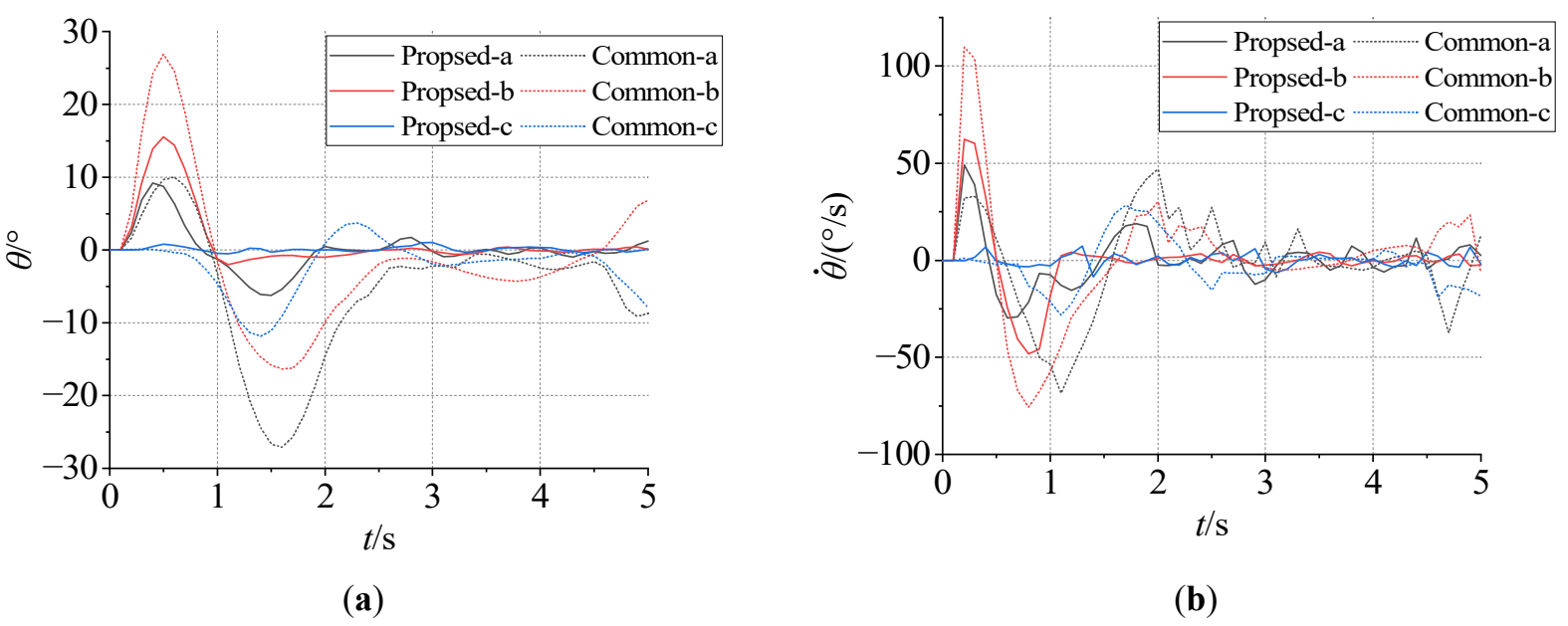
Figure 10. Angle and angular velocity planning results. (a) Pitch angle variation. (b) Pitch angular velocity variation.
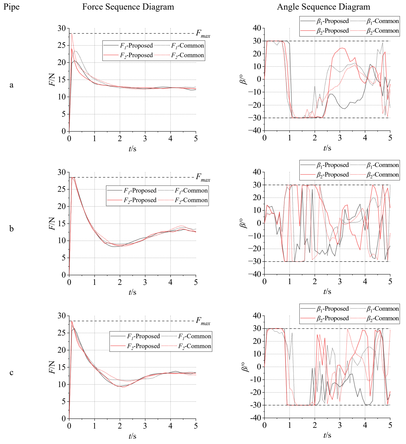
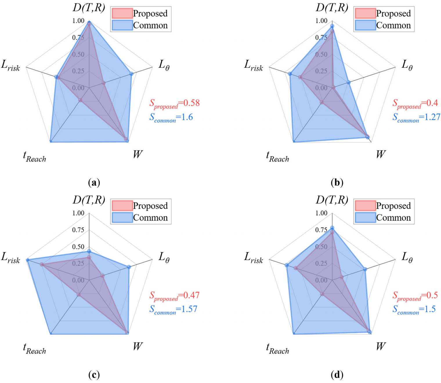
Figure 12. Radar Chart Comparison. (a) Horizontal pipeline. (b) Vertical pipeline. (c) S-shaped pipeline. (d) Comprehensive results.
Table 3. Summary of Evaluation Indicators.
|
Method |
Pipe |
$$\bm{D}\left(\bm{T},\bm{R}\right)$$ |
$${\bm{L}}_{\bm{\theta }}$$ |
$$\bm{\Delta }\bm{\theta }/°$$ |
$$\bar{\boldsymbol{\theta}}/°$$ |
$$\bm{W}/\bm{J}$$ |
$${\bm{t}}_{\bm{r}\bm{e}\bm{a}\bm{c}\bm{h}}/\bm{s}$$ |
$${\bm{L}}_{\bm{r}\bm{i}\bm{s}\bm{k}}$$ |
$${\bm{D}}_{\bm{m}\bm{i}\bm{n}}/\bm{m}$$ |
$$\bar{\boldsymbol{D}}/\boldsymbol{m}$$ |
|---|---|---|---|---|---|---|---|---|---|---|
|
Proposed |
a |
0.28 |
24.5 |
15.4 |
9.1 |
2701 |
2.7 |
3.62 |
0.34 |
1.47 |
|
b |
0.79 |
27.2 |
17.6 |
9.6 |
2616 |
2.3 |
2.38 |
0.73 |
0.99 |
|
|
c |
0.7 |
2.9 |
1.6 |
1.3 |
2496 |
2.7 |
2.48 |
0.7 |
0.95 |
|
|
Average |
0.59 |
18.2 |
11.53 |
6.67 |
2604 |
2.57 |
2.83 |
0.59 |
1.14 |
|
|
Conventional |
a |
0.36 |
74.4 |
37.1 |
37.3 |
2789 |
- |
4.73 |
0.25 |
1.37 |
|
b |
0.83 |
79.4 |
43.2 |
36.2 |
2752 |
- |
2.52 |
0.7 |
0.92 |
|
|
c |
0.76 |
30.5 |
15.6 |
14.9 |
2526 |
- |
3.24 |
0.46 |
0.94 |
|
|
Average |
0.65 |
61.43 |
31.97 |
29.47 |
2689 |
- |
3.5 |
0.47 |
1.08 |
Note: $${t}_{reach}$$ being “-” indicates that the requirement was not met within the simulation time.
From the radar charts and evaluation data, it can be observed that when using the objective function proposed in this paper, the radar chart areas decrease on average across all working conditions, with a mean reduction of 6.7%. Meanwhile, all performance indicators improve to varying degrees, indicating that the overall quality of the generated trajectories is enhanced. Specifically, $$D\left(T,R\right)$$ decreases by 9.2%, suggesting that the dynamic trajectories generated are closer to the corridor centerline. Furthermore, differences in trajectory shape and attitude variation are smaller, indicating smoother, more stable motion. Under the vertical-radius-changing condition, trajectories generated by the proposed objective function are closer to the corridor’s centerline in the constricted section, particularly in the shrinking region, thereby significantly improving trajectory safety. The proposed pitch variation index $${L}_{\theta }$$ is considerably reduced compared with the conventional quadratic objective function, by 70.4%. Specifically, $$\mathrm{\Delta }\theta$$ decreases from 31.97° by 11.53° (a 63.9% reduction), and $$\bar{\theta }$$ decreases from 29.47° by 6.67° (a 77.4% reduction). It can also be seen that, under all test conditions, the upper and lower bounds of the pitch angle appear at approximately the same time (0–2 s). Both the proposed and the conventional cost functions maintain the same timing characteristics, but the pitch-angle extremes in the proposed method are smaller. This shows that the proposed objective function reduces unnecessary oscillations, leading to smoother attitude transitions and improved flight stability. The total energy consumption $$W$$ decreases by 3.1%. Since the propeller thrust varies smoothly under all conditions, this demonstrates that the proposed method achieves more efficient energy use than the conventional quadratic objective. Regarding the time to reach the target, $${t}_{reach}$$ shows a smaller deviation; when using the conventional quadratic cost, the average convergence time is 2.57 s, whereas the proposed method converges in 2.1 s, indicating faster trajectory convergence. The trajectory risk index $${L}_{risk}$$ decreases by 7.1%, indicating that the generated trajectories have better safety margins and smoother proximity to the corridor boundaries. The minimum distance $${D}_{min}$$ increases by an average of 0.12 m, and the average distance $$\bar{D}$$ increases by 0.06 m, showing that the generated trajectories maintain safer clearance from obstacles. In summary, the objective function proposed in this paper effectively reduces attitude variation, improves the trajectory’s approach speed to the target state, and enhances overall stability, rapidity, and safety during flight.
3.3. Comparison with Quadcopter UAVs
For comparison, the trajectory diagrams (Figure 13), state change sequences (Figure 14 and Figure 15), input change sequences (Figure 16), evaluation metrics (Table 4), and radar charts (Figure 17) of a quadcopter under the same parameters across the aforementioned three operating conditions are shown below.
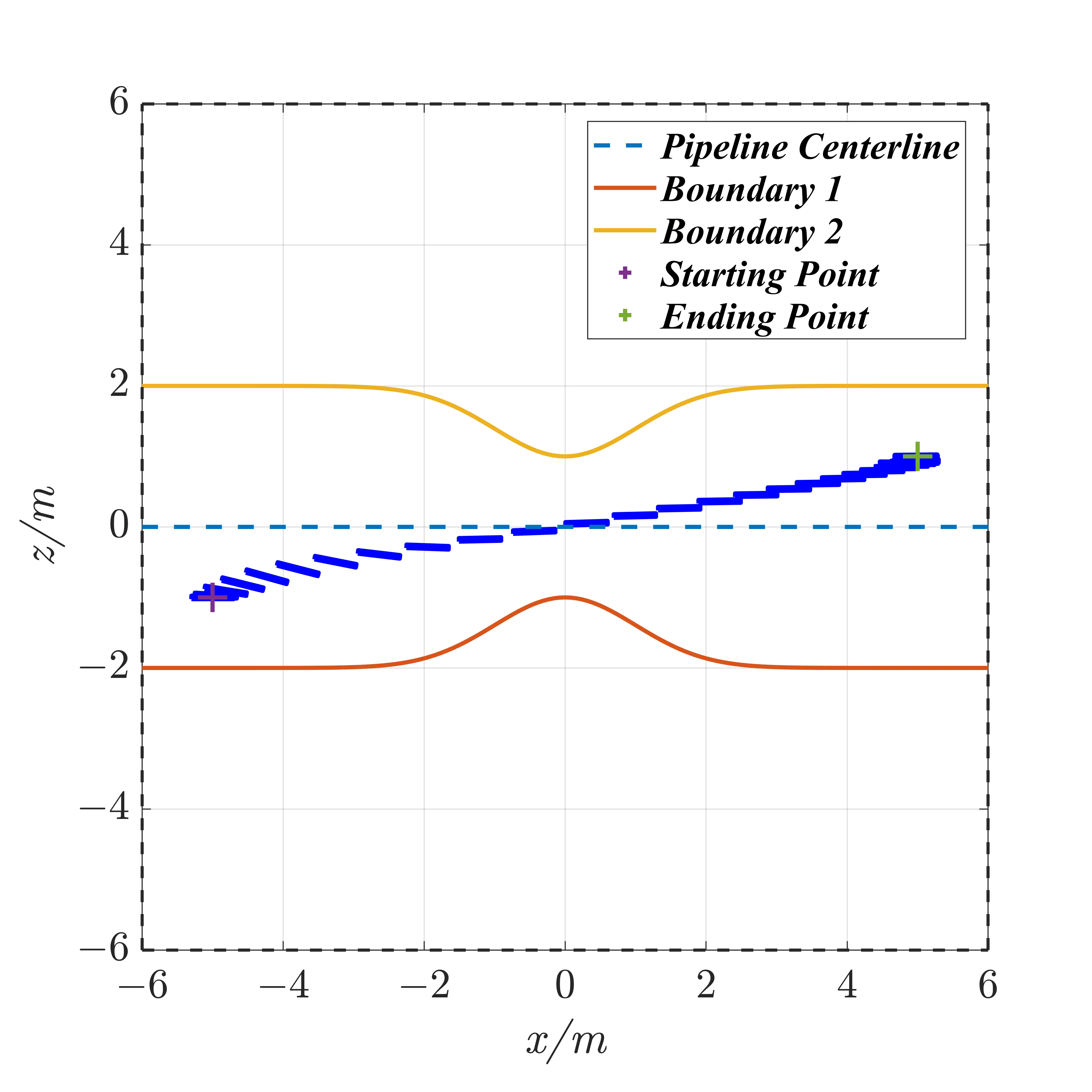
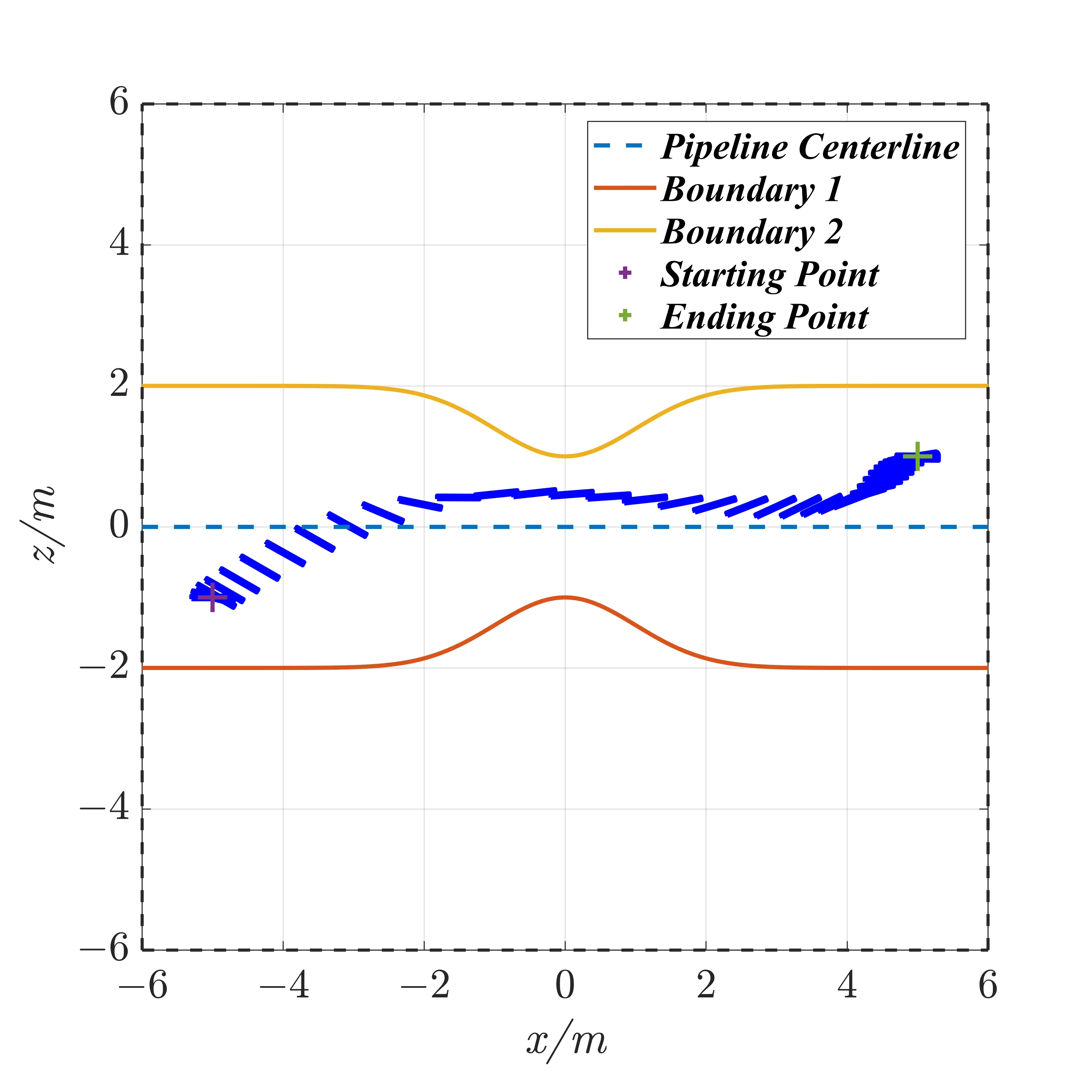
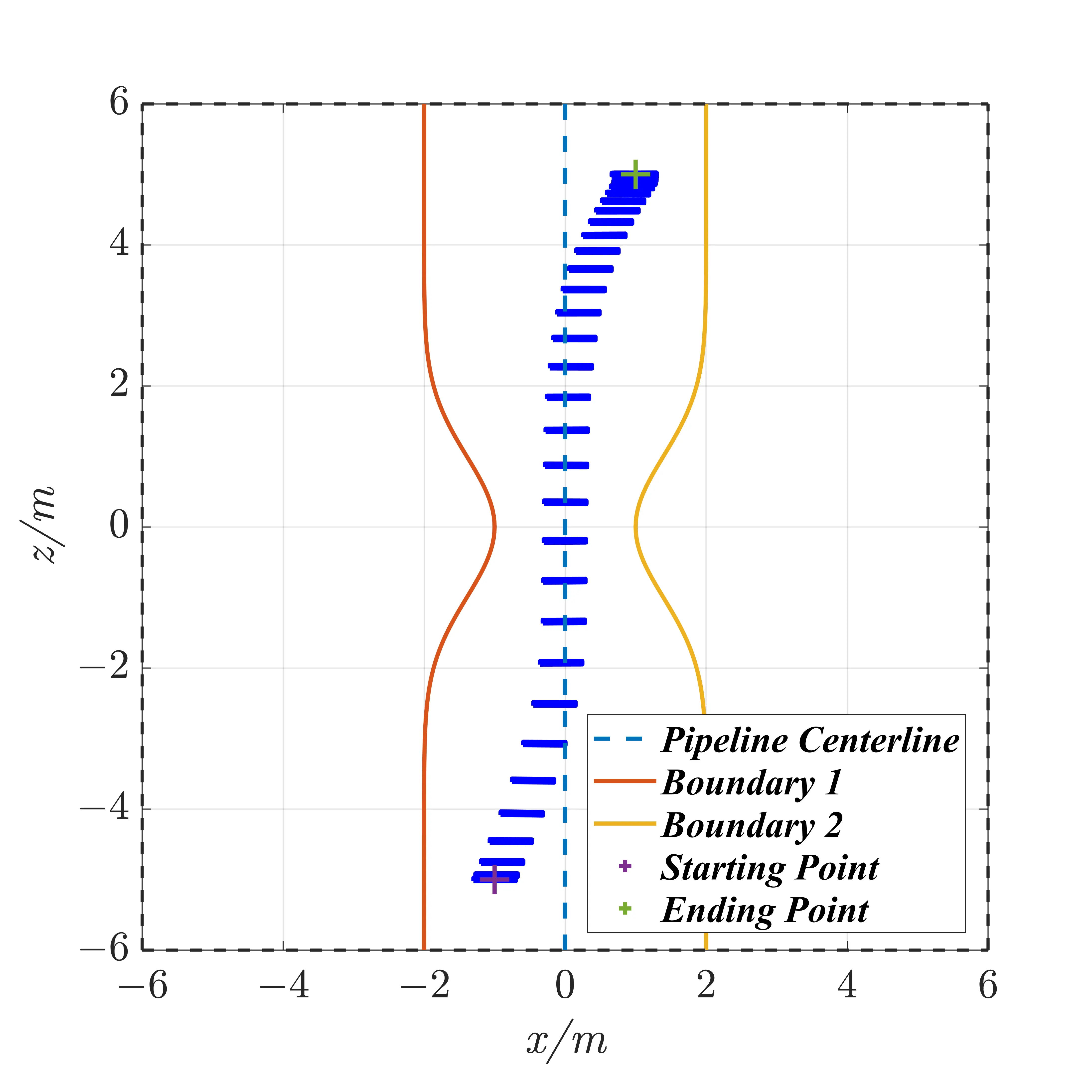
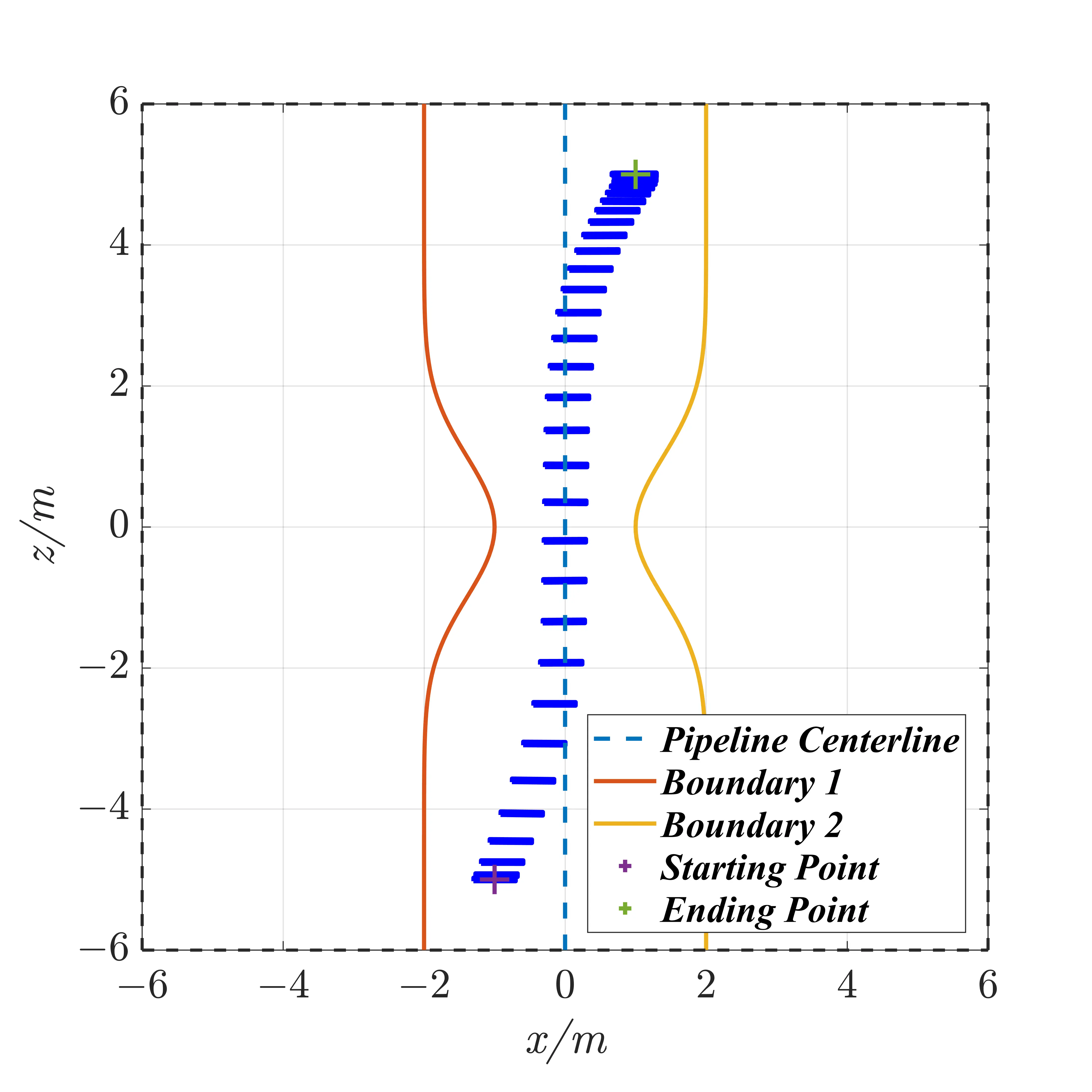
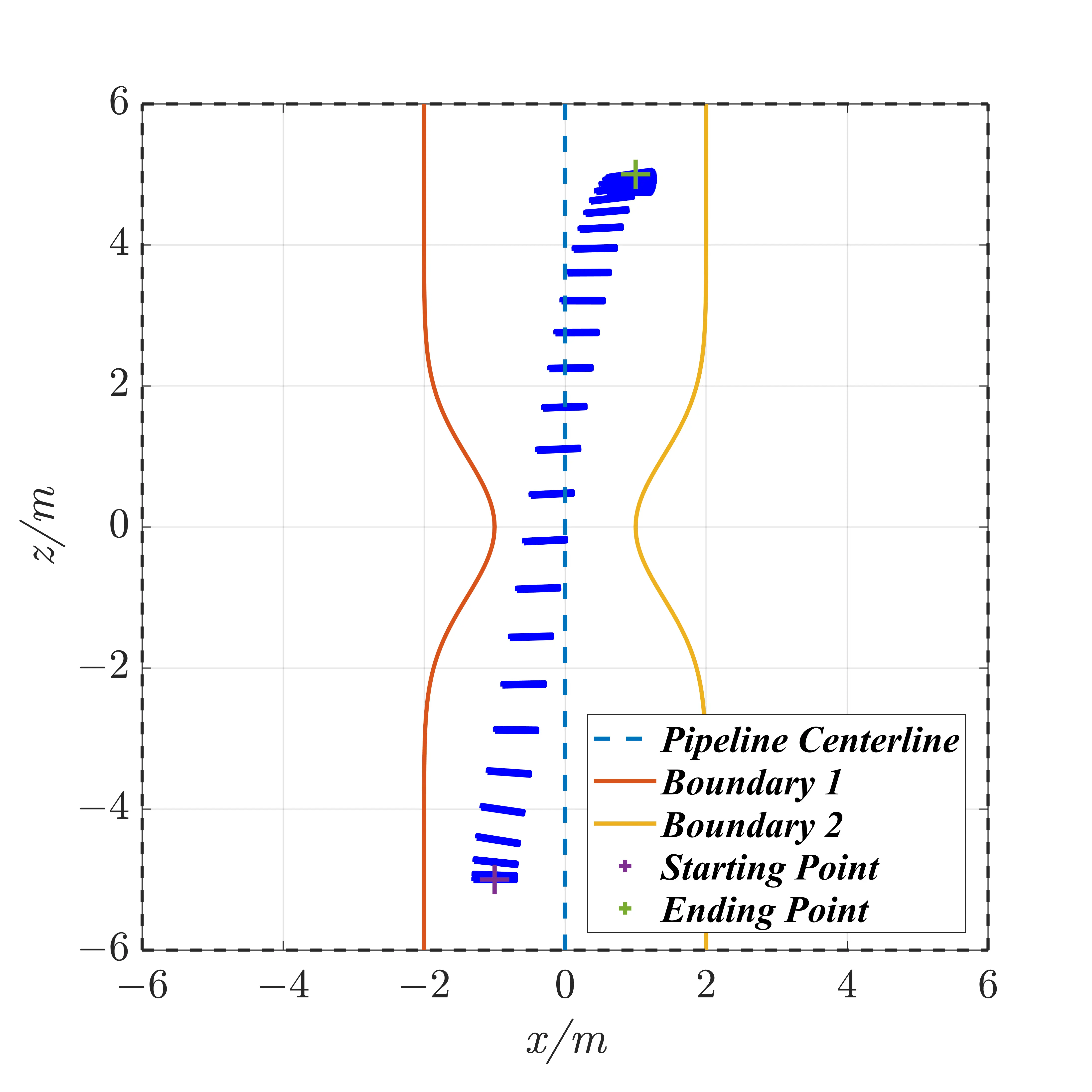
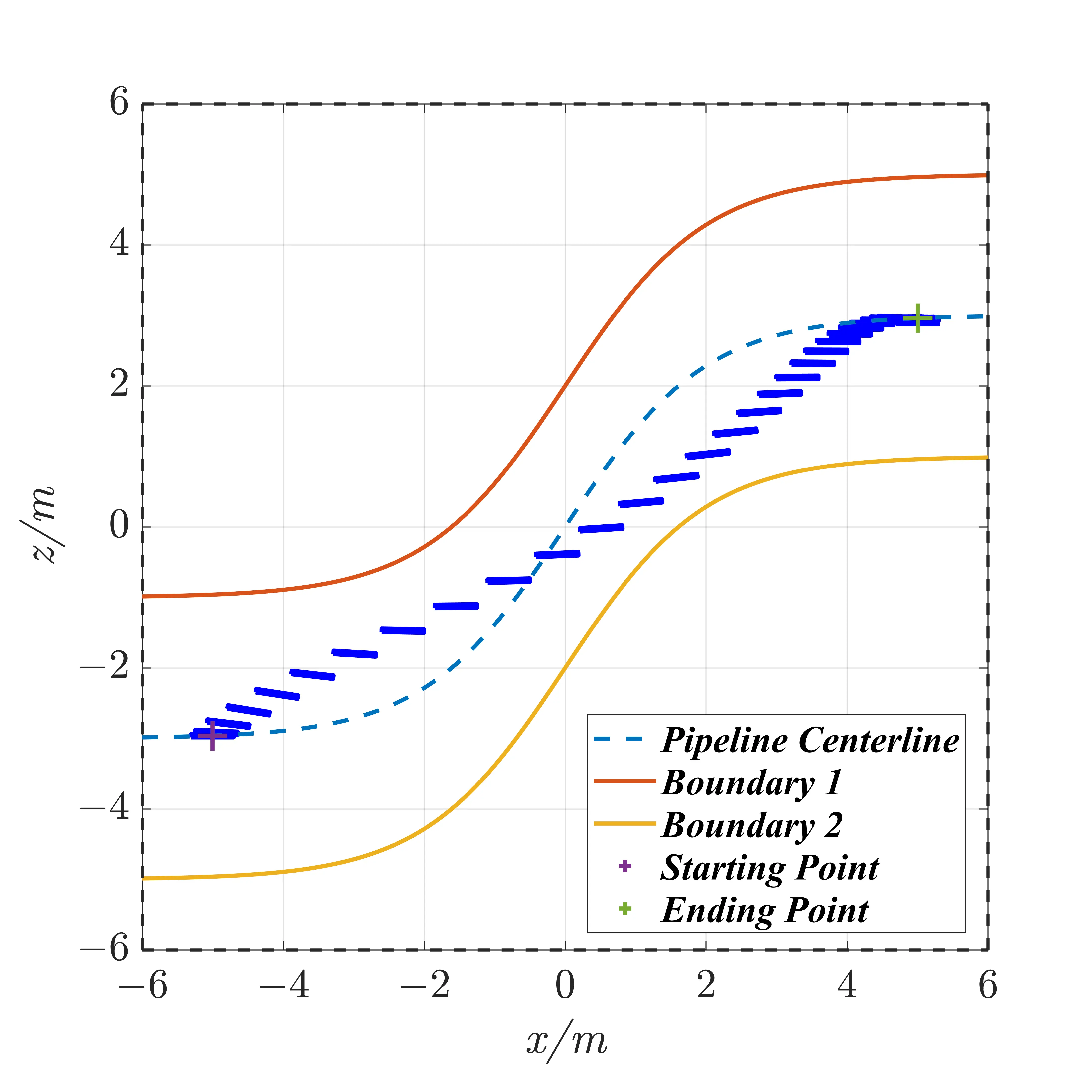
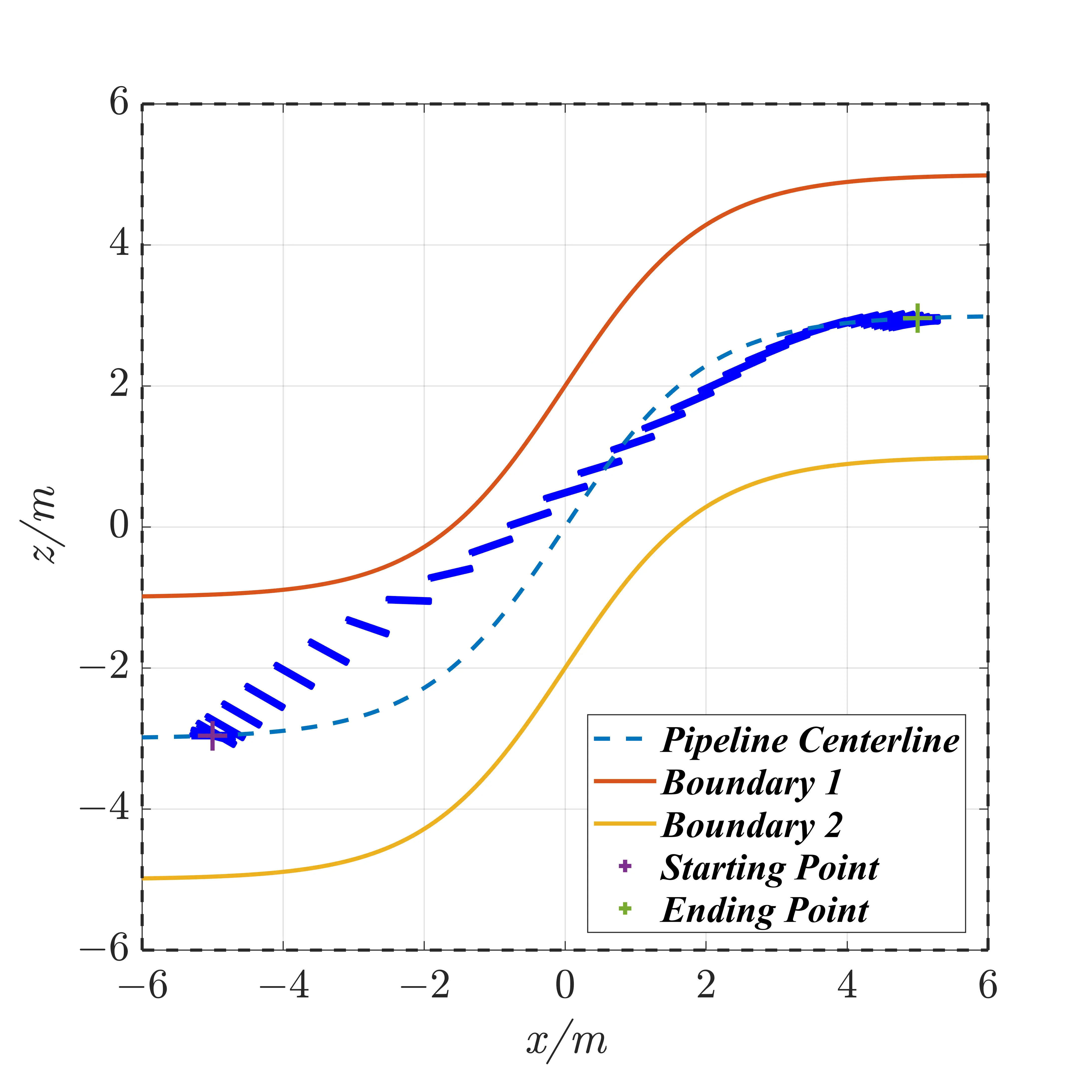
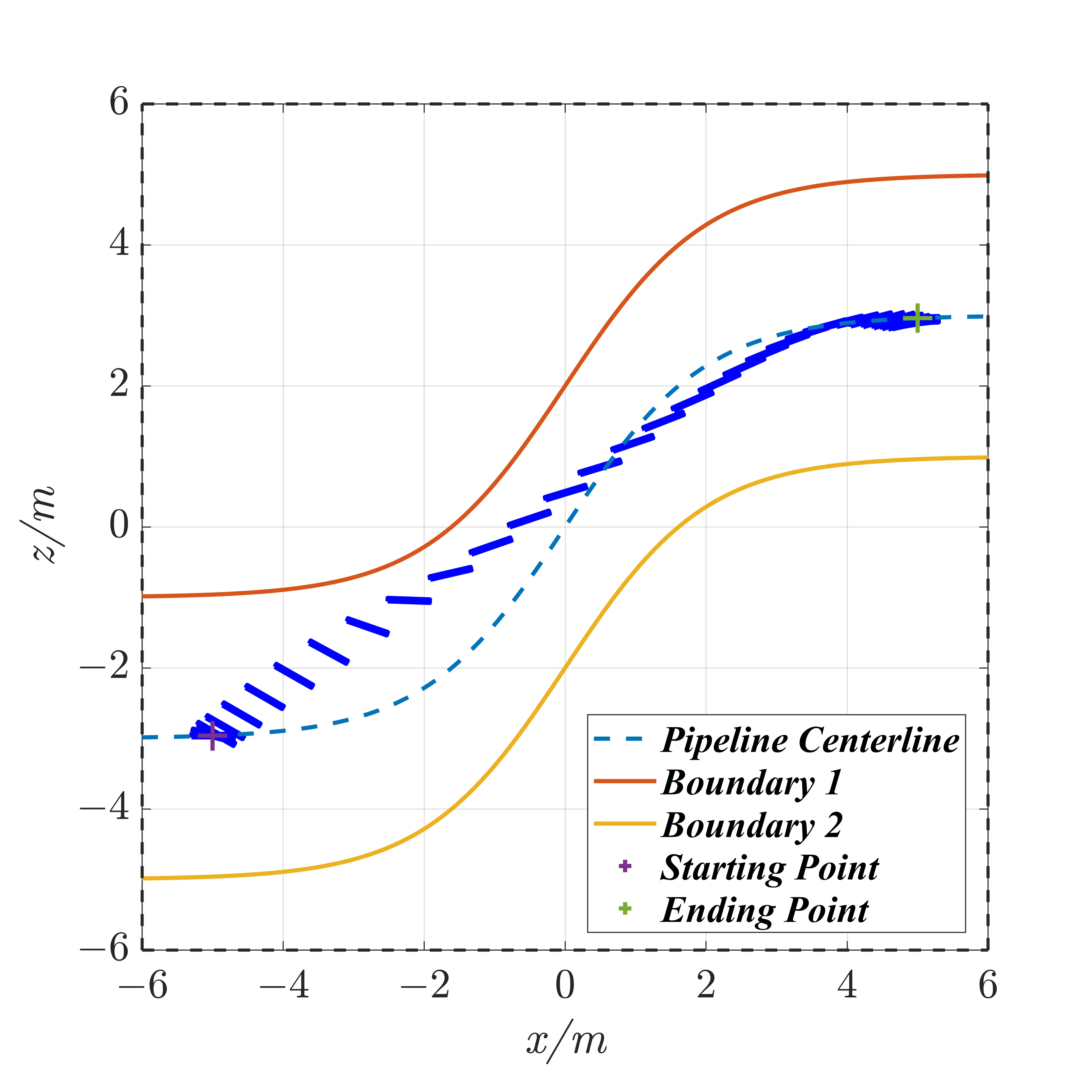
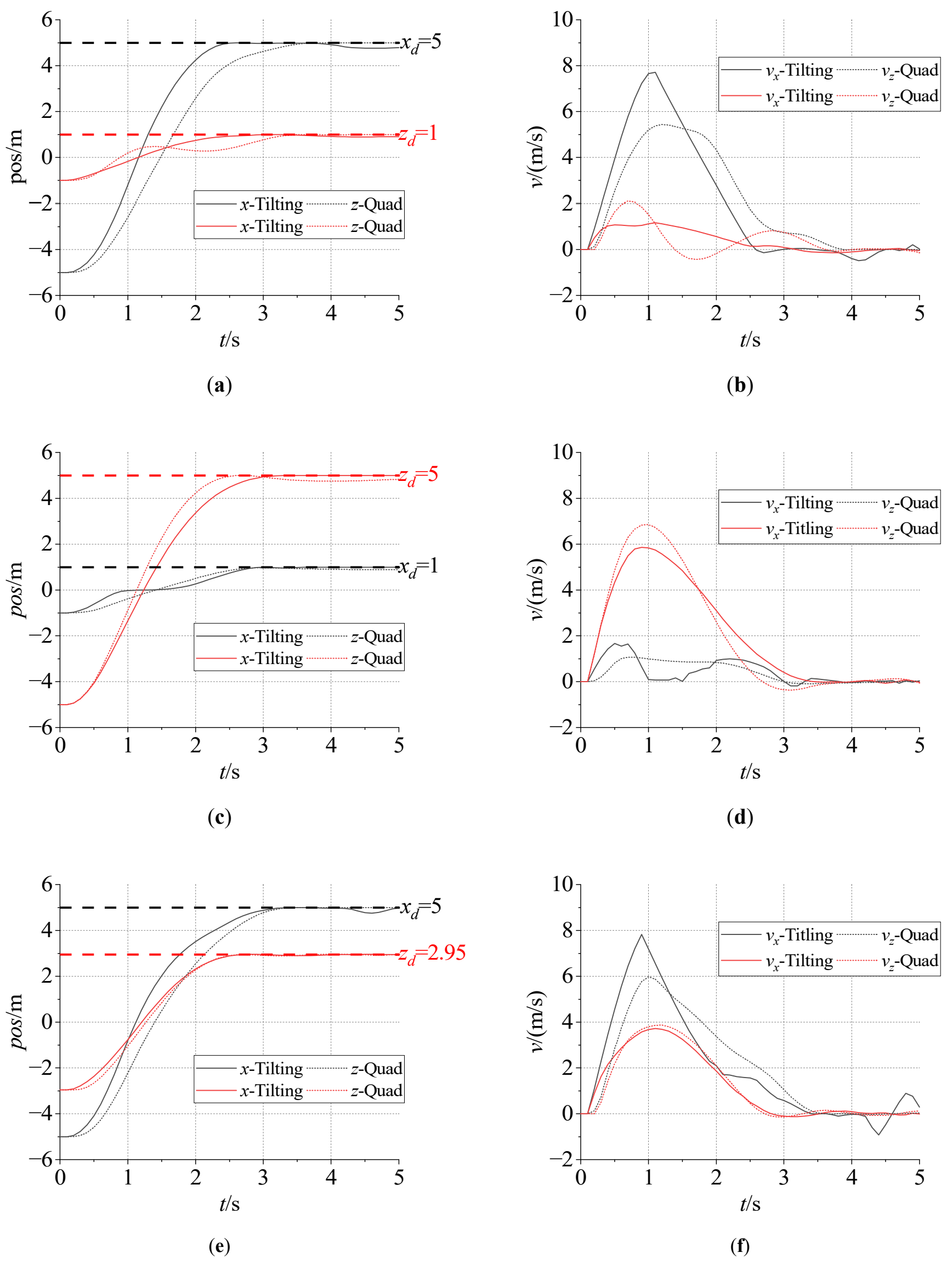
Figure 14. Position and Attitude Planning Results. (a) Position of the transverse pipeline. (b) Velocity of the transverse pipeline. (c) Position of the vertical pipeline. (d) Velocity of the vertical pipeline. (e) Position of the S-pipeline. (f) Velocity of the S-pipeline.
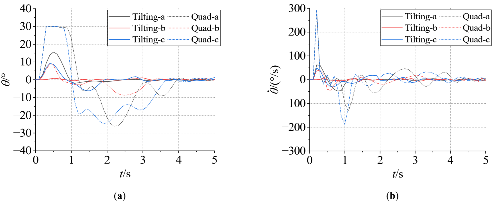
Figure 15. Angle and angular velocity planning results. (a) Pitch angle variation. (b) Pitch angular velocity variation.
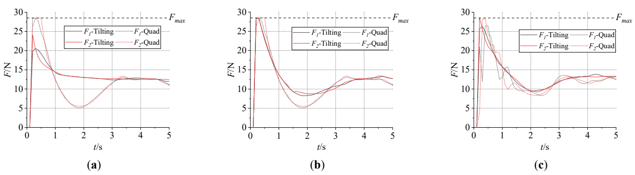
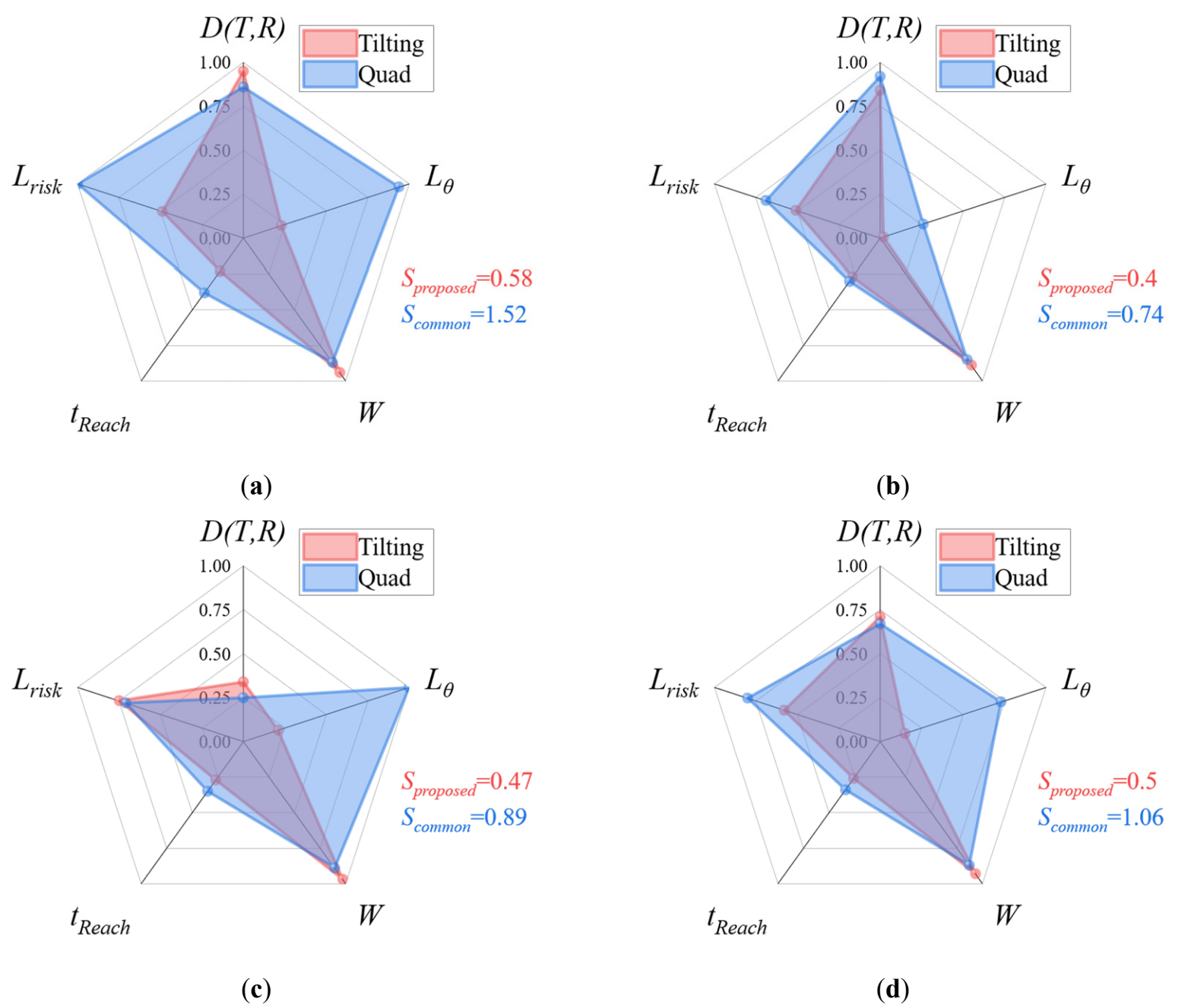
Figure 17. Radar Chart Comparison. (a) Horizontal pipeline. (b) Vertical pipeline. (c) S-shaped pipeline. (d) Comprehensive results.
Table 4. Summary of Evaluation Indicators.
|
Platform |
Pipe |
$$\bm{D}\left(\bm{T},\bm{R}\right)$$ |
$${\bm{L}}_{\bm{\theta }}$$ |
$$\bm{\Delta }\bm{\theta }\bm{/°}$$ |
$$\bar{\bm{\theta }}\bm{/°}$$ |
$$\bm{W}/\bm{J}$$ |
$${\bm{t}}_{\bm{r}\bm{e}\bm{a}\bm{c}\bm{h}}/\bm{s}$$ |
$${\bm{L}}_{\bm{r}\bm{i}\bm{s}\bm{k}}$$ |
$${\bm{D}}_{\bm{m}\bm{i}\bm{n}}/\bm{m}$$ |
$$\bar{\boldsymbol{D}}/\boldsymbol{m}$$ |
|---|---|---|---|---|---|---|---|---|---|---|
|
Thrust-vectoring |
a |
0.28 |
24.5 |
15.4 |
9.1 |
2701 |
2.7 |
3.62 |
0.34 |
1.47 |
|
b |
0.79 |
27.2 |
17.6 |
9.6 |
2616 |
2.3 |
2.38 |
0.73 |
0.99 |
|
|
c |
0.7 |
2.9 |
1.6 |
1.3 |
2496 |
2.7 |
2.48 |
0.7 |
0.95 |
|
|
Average |
0.59 |
18.2 |
11.53 |
6.67 |
2604 |
2.57 |
2.83 |
0.59 |
1.14 |
|
|
Quadrotor |
a |
0.21 |
118.4 |
54.6 |
63.8 |
2481 |
3.5 |
3.44 |
0.36 |
1.5 |
|
b |
0.71 |
111.3 |
56.1 |
55.2 |
2418 |
3.8 |
4.85 |
0.26 |
1 |
|
|
c |
0.76 |
30.8 |
17.7 |
13.1 |
2374 |
3 |
3.35 |
0.44 |
0.93 |
|
|
Average |
0.56 |
86.83 |
42.8 |
44.03 |
2424 |
3.43 |
3.88 |
0.35 |
1.14 |
From the radar charts and comparison data, it can be seen that under all test conditions, the radar chart area corresponding to the thrust-vectoring aircraft proposed in this paper is smaller than that of the conventional quadrotor. The average radar chart area decreases by 52.8%, indicating that the proposed thrust-vectoring aircraft achieves better trajectory performance. Specifically, the difference in $$D\left(T,R\right)$$ between the two platforms is small, indicating that both trajectories remain close to the ideal reference path. However, the thrust-vectoring aircraft exhibits smoother directional changes during motion, enabling more flexible, continuous trajectory transitions. From the lateral and vertical trajectories, it can be observed that the thrust-vectoring aircraft’s trajectory transitions are more gradual. The vehicle naturally adjusts its pitch angle when moving along curved paths, aligning its body axis with the reference trajectory and achieving smoother turns compared with the quadrotor, whose pitch motion lags behind slightly. For the S-shaped path, the thrust-vectoring aircraft’s trajectory closely follows the ideal path with smoother curvature transitions, while the quadrotor deviates more in the middle and end segments. Moreover, the thrust-vectoring aircraft shows a significant reduction in the attitude variation index $${L}_{\theta }$$, decreasing by 79.0%. Specifically, $$\mathrm{\Delta }\theta$$ and $$\bar{\theta }$$ are reduced by 73.1% and 84.9%, respectively, indicating a large reduction in attitude variation and improved overall stability. The pitch-angle variation curves further confirm this result: the quadrotor’s pitch angle changes rapidly within 0–1 s, while the thrust-vectoring aircraft’s pitch remains within ±5° after 1 s, maintaining steady flight. In contrast, the quadrotor continues to oscillate around ±20°, with the oscillations persisting for more than 2 s. Additionally, from the pitch rate curves, the thrust-vectoring aircraft’s angular velocity fluctuations are smaller, typically within ±100°/s, whereas the quadrotor exhibits pitch rate peaks exceeding 300°/s, suggesting that the thrust-vectoring configuration achieves smoother and more controlled motion. Regarding energy consumption, the thrust-vectoring aircraft maintains an average thrust of around 25 N, without any overshoot observed in the quadrotor. The thrust-vectoring aircraft also demonstrates better energy efficiency and smoother power transitions between rotors, while maintaining a similar reduction in total energy consumption of 7.1%. For flight safety, the minimum distance $${D}_{min}$$ increases by 0.14 m, and the average distance $$\bar{D}$$ increases by 0.07 m, indicating better obstacle clearance and higher safety margins. The trajectory risk index $${L}_{risk}$$ decreases by 27.1%, showing that the generated paths under the thrust-vectoring configuration are safer and more robust against potential collision risks. In summary, the thrust-vectoring aircraft outperforms the conventional quadrotor in terms of trajectory smoothness, energy efficiency, and safety. The proposed design effectively reduces attitude variations and enhances stability, rapidity, and safety during flight.
Compared with conventional quadratic cost formulations, the proposed multi-objective trajectory generation framework offers greater flexibility for balancing trajectory smoothness, control effort, and obstacle-avoidance performance. By explicitly introducing multiple cost components, the optimization process can better adapt to constrained environments, resulting in smoother trajectories that maintain a safer distance from obstacles. In addition, the proposed formulation enables a unified optimization framework applicable to different UAV configurations, including conventional quadrotors and tilting UAVs, thereby demonstrating broader applicability than existing trajectory generation methods. These results demonstrate the effectiveness of the proposed approach in generating dynamically feasible trajectories in constrained pipeline environments.
4. Discussion
This paper proposes a trajectory generation framework for thrust-vectoring aircraft operating in constrained spaces. By constructing constraint-space parameters, the environmental boundaries are combined with the aircraft’s aerodynamic model to form a constrained optimization problem that accounts for multiple performance indicators. The resulting optimization problem is solved using the SQP algorithm. In simulation experiments across three representative corridor types, the results demonstrate that the proposed method can effectively balance the trade-offs among trajectory rapidity, stability, safety, and energy efficiency. The trajectories generated under this framework exhibit smoother, more coordinated motion and better positional and attitude tracking performance. Compared with the conventional quadratic objective function, the proposed method achieves a significant overall improvement across five key evaluation dimensions. Specifically, the trajectory risk index $${L}_{{risk}}$$ and total energy consumption $$W$$ are reduced by 70.4% and 19.1%, respectively. Meanwhile, $${t}_{reach}$$ showed significant improvement. While conventional quadratic objective functions failed to converge within the simulation time, the proposed method achieved convergence in 2.57 s (out of a total simulation time of 5 s). These results indicate that the proposed approach significantly enhances the overall dynamic stability of trajectory generation and improves trajectory smoothness and flight safety. Furthermore, the proposed approach provides a unified solution framework for thrust-vectoring trajectory generation in constrained environments, making it adaptable to multi-rotor UAVs. Based on the results, the generated trajectories exhibit reduced attitude fluctuations: $$\mathrm{\Delta }\theta$$, $$\bar{\theta }$$, and $${L}_{\theta }$$ are reduced by 79.0%, 25.1%, and 27.1%, respectively, corresponding to a maximum attitude change reduction from $$±{30}^{\circ }$$ to $$±{20}^{\circ }$$. The minimum safety distance $${D}_{min}$$ increases by an average of 68.6%, demonstrating improved safety margins.
Future research will focus on the following aspects: (1) Generalization of the constraint space: Extending the constraint space from two-dimensional ducts to other types of constraint spaces in three-dimensional domains; (2) Incorporation of disturbances: The mutual interference between near-surface effects and the aircraft flow field within the actual constraint space introduces significant uncertainty in motion. How to account for such disturbances in trajectory generation remains an urgent research topic; (3) Universality of the trajectory generation framework: Validating the proposed framework’s applicability across different thrust-vectoring vehicles, including the three typical categories mentioned in the introduction; (4) Algorithm refinement: Enhance the treatment of objective functions and constraints within the algorithm, particularly the computation and evaluation of distances to environmental boundaries. Consider adopting more efficient computational approaches (e.g., improvements to signed distance fields); (5) Experimental validation: Develop a physical prototype, implement the trajectory generation method, and conduct experimental validation within a real-world constrained space environment.
5. Conclusions
This paper proposes a multi-objective optimization-based trajectory generation framework for thrust-vectoring aircraft operating within constrained spaces. The proposed method comprehensively considers both environmental boundary constraints and the dynamic characteristics of thrust-vectoring aircraft, addressing multiple performance objectives, including safety, stability, rapidity, and energy efficiency. Compared with the conventional quadratic optimization approach, the proposed method significantly reduces attitude variation and trajectory risk, with $${L}_{\theta }$$ and $${L}_{{risk}}$$ decreasing by 70.4% and 19.1%, respectively. Meanwhile, the aircraft’s attitude states converge to the desired condition within the prescribed time. When compared with a conventional quadrotor, the proposed thrust-vectoring aircraft achieves further improvements, with $${L}_{\theta }$$, $${t}_{reach}$$, and $${L}_{{risk}}$$ reduced by 79.0%, 25.1%, and 27.1%, respectively. The trajectory exhibits smaller attitude variations and generates more optimized flight paths, fully leveraging the decoupling advantages of thrust-vectoring aircraft. Future research will focus on extending the framework to more complex constrained-space modeling, enhancing algorithms, and conducting experimental validation.
Statement of the Use of Generative AI and AI-Assisted Technologies in the Writing Process
During the preparation of this manuscript, the authors used ChatGPT for language polishing. After using this tool, the authors reviewed and edited the content as needed and take full responsibility for the content of the published article.
Author Contributions
Y.S.: Software, Formal analysis, Writing—Original Draft. W.W.: Conceptualization, Methodology, Supervision, Resources. M.D.: Investigation, Writing—Review & Editing. Y.W.: Investigation, Validation. X.Z.: Data Curation. J.L.: Investigation.
Ethics Statement
Not applicable.
Informed Consent Statement
Not applicable.
Data Availability Statement
The data supporting the findings of this study are available from the corresponding author upon reasonable request.
Funding
This research received no external funding. The APC was funded by the Beijing Natural Science Foundation (3244036), the National Key Research and Development Program of China (2020YFC1512500), the Shandong Postdoctoral Innovation Project (SDCX-ZG-202303052), and the General Program of the Chongqing Natural Science Foundation (CSTB2022NSCQ-MSX1101).
Declaration of Competing Interest
The authors declare that they have no known competing financial interests or personal relationships that could have appeared to influence the work reported in this paper.
References
-
Wei W, Shu Y, Liu J, Dong L, Jia L, Wang J, et al. Research on a hierarchical feature-based contour extraction method for spatial complex truss-like structures in aerial images. Eng. Appl. Artif. Intell. 2024, 127, 107313. DOI:10.1016/j.engappai.2023.107313 [Google Scholar]
-
Brescianini D, D’Andrea R. Tilt-Prioritized Quadrocopter Attitude Control. IEEE Trans. Control Syst. Technol. 2020, 28, 376–387. DOI:10.1109/TCST.2018.2873224 [Google Scholar]
-
Wei W, Shu Y, Ke Z, Fan K, Dong L. Study on Roll Oscillation Phenomenon and Controller Design of Deflection-based Flying Vehicles. In Proceedings of the 2023 10th International Conference on Dependable Systems and Their Applications (DSA), Tokyo, Japan, 10–11 August 2023; pp. 800–809. DOI:10.1109/DSA59317.2023.00113 [Google Scholar]
-
Bamert S, Cathomen R, Gorlo N, Käppeli G, Müller MS, Reinhart T, et al. Geranos: A Novel Tilted-Rotors Aerial Robot for the Transportation of Poles. IEEE Robot. Autom. Mag. 2024, 31, 66–77. DOI:10.1109/MRA.2023.3348306 [Google Scholar]
-
Dong X, Cui Y, Xiang J, Li D, Tu Z. An Efficient Trajectory Generation for Bi-copter Flight in Tight Space. arXiv 2024, arXiv:2406.00671. DOI:10.48550/arXiv.2406.00671 [Google Scholar]
-
Rashad R, Goerres J, Aarts R, Engelen JBC, Stramigioli S. Fully Actuated Multirotor UAVs: A Literature Review. IEEE Robot. Autom. Mag. 2020, 27, 97–107. DOI:10.1109/MRA.2019.2955964 [Google Scholar]
-
Hamandi M, Usai F, Sablé Q, Staub N, Tognon M, Franchi A. Design of multirotor aerial vehicles: A taxonomy based on input allocation. Int. J. Robot. Res. 2021, 40, 1015–1044. DOI:10.1177/02783649211025998 [Google Scholar]
-
Hameed SW, Imanberdiyev N, Camci E, Yau W-Y, Feroskhan M. Bio-inspired classification and evolution of multirotor Micro Aerial Vehicles (MAVs): A comprehensive review. Robot. Auton. Syst. 2024, 182, 104802. DOI:10.1016/j.robot.2024.104802 [Google Scholar]
-
Park S, Lee J, Ahn J, Kim M, Her J, Yang G-H, et al. ODAR: Aerial Manipulation Platform Enabling Omnidirectional Wrench Generation. IEEE/ASME Trans. Mechatron. 2018, 23, 1907–1918. DOI:10.1109/TMECH.2018.2848255 [Google Scholar]
-
Allenspach M, Bodie K, Brunner M, Rinsoz L, Taylor Z, Kamel M, et al. Design and optimal control of a tiltrotor micro-aerial vehicle for efficient omnidirectional flight. Int. J. Robot. Res. 2020, 39, 1305–1325. DOI:10.1177/0278364920943654 [Google Scholar]
-
Hamandi M, Ali AM, Evangeliou N, Chaikalis D, Tzes A, Kyriakopoulos K, et al. Mechatronic Design of an Omnidirectional Octorotor UAV. In Proceedings of the 2024 10th International Conference on Automation, Robotics and Applications (ICARA), Athens, Greece, 22–24 February 2024; pp. 300–304. DOI:10.1109/ICARA60736.2024.10553043 [Google Scholar]
-
Iriarte I, Otaola E, Culla D, Iglesias I, Lasa J, Sierra B. Modeling and control of an overactuated aerial vehicle with four tiltable quadrotors attached by means of passive universal joints. In Proceedings of the 2020 International Conference on Unmanned Aircraft Systems (ICUAS), Athens, Greece, 1–4 September 2020; pp. 1748–1756. DOI:10.1109/ICUAS48674.2020.9213848 [Google Scholar]
-
Shi C, Wang K, Yu Y. Expandable Fully Actuated Aerial Vehicle Assembly: Geometric Control Adapted from an Existing Flight Controller and Real-World Prototype Implementation. Drones 2022, 6, 272. DOI:10.3390/drones6100272 [Google Scholar]
-
Qin Y, Chen N, Cai Y, Xu W, Zhang F, Zhang F. Gemini II: Design, Modeling, and Control of a Compact Yet Efficient Servoless Bi-copter. IEEE/ASME Trans. Mechatron. 2022, 27, 4304–4315. DOI:10.1109/TMECH.2022.3153587 [Google Scholar]
-
Sakaguchi A, Takimoto T, Ushio T. A Novel Quadcopter with A Tilting Frame using Parallel Link Mechanism. In Proceedings of the 2019 International Conference on Unmanned Aircraft Systems (ICUAS), Atlanta, GA, USA, 11–14 June 2019; pp. 674–683. DOI:10.1109/ICUAS.2019.8797934 [Google Scholar]
-
Zheng P, Tan X, Kocer BB, Yang E, Kovac M. TiltDrone: A Fully-Actuated Tilting Quadrotor Platform. IEEE Robot. Autom. Lett. 2020, 5, 6845–6852. DOI:10.1109/LRA.2020.3010460 [Google Scholar]
-
Ryll M, Bicego D, Giurato M, Lovera M, Franchi A, Hexarotor AM, et al. Control and Experimental Validation. IEEE/ASME Trans. Mechatron. 2022, 27, 1244–1255. DOI:10.1109/TMECH.2021.3099197 [Google Scholar]
-
Kamel M, Verling S, Elkhatib O, Sprecher C, Wulkop P, Taylor Z, et al. The Voliro Omniorientational Hexacopter: An Agile and Maneuverable Tiltable-Rotor Aerial Vehicle. IEEE Robot. Autom. Mag. 2018, 25, 34–44. DOI:10.1109/MRA.2018.2866758 [Google Scholar]
-
Cuniato E, Geckeler C, Brunner M, Strübin D, Bähler E, Ospelt F, et al. Design and Control of a Micro Overactuated Aerial Robot with an Origami Delta Manipulator. In Proceedings of the 2023 IEEE International Conference on Robotics and Automation (ICRA), London, UK, 29 May–2 June 2023; pp. 5352–5358. DOI:10.1109/ICRA48891.2023.10161060 [Google Scholar]
-
Yang Y, Yu X, Li Z, Basin MV. A New Overactuated Multirotor: Prototype Design, Dynamics Modeling, and Control. IEEE Trans. Ind. Electron. 2024, 71, 9449–9459. DOI:10.1109/TIE.2023.3314924 [Google Scholar]
-
Zhou X, Wang Z, Ye H, Xu C, Gao F. EGO-Planner: An ESDF-Free Gradient-Based Local Planner for Quadrotors. IEEE Robot. Autom. Lett. 2021, 6, 478–485. DOI:10.1109/LRA.2020.3047728 [Google Scholar]
-
Zhou B, Pan J, Gao F, Shen S. RAPTOR: Robust and Perception-aware Trajectory Replanning for Quadrotor Fast Flight. IEEE Trans. Robot. 2021, 37, 1992–2009. DOI:10.1109/TRO.2021.3071527 [Google Scholar]
-
Zhou B, Gao F, Wang L, Liu C, Shen S. Robust and Efficient Quadrotor Trajectory Generation for Fast Autonomous Flight. IEEE Robot. Autom. Lett. 2019, 4, 3529–3536. DOI:10.1109/LRA.2019.2927938 [Google Scholar]
-
Han Z, Wang Z, Pan N, Lin Y, Xu C, Gao F. Fast-Racing: An Open-Source Strong Baseline for SE(3) Planning in Autonomous Drone Racing. IEEE Robot. Autom. Lett. 2021, 6, 8631–8638. DOI:10.1109/LRA.2021.3113976 [Google Scholar]
-
Selin M, Tiger M, Duberg D, Heintz F, Jensfelt P. Efficient Autonomous Exploration Planning of Large-Scale 3-D Environments. IEEE Robot. Autom. Lett. 2019, 4, 1699–1706. DOI:10.1109/LRA.2019.2897343 [Google Scholar]
-
Liu P, Shen Y, Liu Y, Quan F, Wang C, Chen H. Generating 6-D Trajectories for Omnidirectional Multirotor Aerial Vehicles in Cluttered Environments. IEEE Robot. Autom. Lett. 2024, 9, 8818–8825. DOI:10.1109/LRA.2024.3448135 [Google Scholar]
-
Liu P, Quan F, Liu Y, Chen H. Collision-Free 6-DoF Trajectory Generation for Omnidirectional Multi-rotor Aerial Vehicle. arXiv 2022, arXiv:2209.06764. DOI:10.48550/arXiv.2209.06764 [Google Scholar]
-
Liu K, Ma L, Zhou H, Li S, Zhang K, Huang D, et al. Optimal Time Trajectory Generation and Tracking Control for Over-actuated Multirotors with Large-angle Maneuvering Capability. IEEE Robot. Autom. Lett. 2022, 7, 8339–8346. DOI:10.1109/LRA.2022.3187260 [Google Scholar]
-
Hamandi M, Al-Ali I, Seneviratne L, Franchi A, Zweiri Y. Full-Pose Trajectory Tracking of Overactuated Multi-Rotor Aerial Vehicles with Limited Actuation Abilities. IEEE Robot. Autom. Lett. 2023, 8, 4951–4958. DOI:10.1109/LRA.2023.3290422 [Google Scholar]
-
Hachem M, Miquel T, Bronz M, Roos C. Trajectory Optimization for Fully Actuated Hexacopters: Enhancing Maneuverability and Applications. 2023. Available online: https://enac.hal.science/hal-04396701 (accessed on 27 March 2025).
-
Su Y, Li J, Jiao Z, Wang M, Chu C, Li H, et al. Sequential Manipulation Planning for Over-Actuated UAMs. In Proceedings of the 2023 IEEE/RSJ International Conference on Intelligent Robots and Systems (IROS), Detroit, MI, USA, 1–5 October 2023. [Google Scholar]
-
Su Y, Zhang J, Jiao Z, Li H, Wang M, Liu H. Real-time Dynamic-consistent Motion Planning for Over-actuated UAVs. In Proceedings of the 2024 IEEE International Conference on Robotics and Automation (ICRA), Yokohama, Japan, 13–17 May 2024; pp. 11789–11795. DOI:10.1109/ICRA57147.2024.10610236 [Google Scholar]
-
Allenspach M, Laasch S, Lawrance N, Tognon M, Siegwart R. Mixed Reality Human-Robot Interface to Generate and Visualize 6DoF Trajectories: Application to Omnidirectional Aerial Vehicles. In Proceedings of the 2023 International Conference on Unmanned Aircraft Systems (ICUAS), Warsaw, Poland, 6–9 June 2023; pp. 395–400. DOI:10.1109/ICUAS57906.2023.10156523 [Google Scholar]
-
Mandralis I, Sihite E, Ramezani A, Gharib M. Minimum Time Trajectory Generation for Bounding Flight: Combining Posture Control and Thrust Vectoring. In Proceedings of the 2023 European Control Conference (ECC), Bucharest, Romania, 13–16 June 2023; pp. 1–7. DOI:10.23919/ECC57647.2023.10178360 [Google Scholar]
-
Liu K, Zheng J. UAV Trajectory Optimization for Time-Constrained Data Collection in UAV-Enabled Environmental Monitoring Systems. IEEE Internet Things J. 2022, 9, 24300–24314. DOI:10.1109/JIOT.2022.3189214 [Google Scholar]
-
Memos VA, Psannis KE. Optimized UAV-based data collection from MWSNs. ICT Express 2023, 9, 29–33. DOI:10.1016/j.icte.2022.10.003 [Google Scholar]
-
Cui J, Ding Z, Deng Y, Nallanathan A, Hanzo L. Adaptive UAV-Trajectory Optimization Under Quality of Service Constraints: A Model-Free Solution. IEEE Access 2020, 8, 112253–112265. DOI:10.1109/ACCESS.2020.3001752 [Google Scholar]
-
Shu Y, Dong L, Liu J, Liu C, Wei W. Overview of Terrain Traversability Evaluation for Autonomous Robots. J. Field Robot. 2024, 42, 1724–1765. DOI:10.1002/rob.22461 [Google Scholar]