
Dispersion During Underground Hydrogen Storage in Depleted Gas Reservoirs

Dispersion During Underground Hydrogen Storage in Depleted Gas Reservoirs

Received: 19 January 2026 Revised: 18 March 2026 Accepted: 20 April 2026 Published: 06 May 2026

© 2026 The authors. This is an open access article under the Creative Commons Attribution 4.0 International License (https://creativecommons.org/licenses/by/4.0/).
1. Introduction
Hydrogen (H2) is gaining consideration as a low-carbon energy carrier for decarbonizing transportation, heat, and power, and fuel-intensive industries [1]. Large-scale underground storage of hydrogen gas is expected to play a key role in the energy transition and, in the near future, renewable energy systems [2], because natural fluctuations in energy production from renewable sources can lead to supply shortages. One of the ways to address the shortages is to store large quantities of excess energy in the form of hydrogen, over long timescales [3]. Hydrogen can be stored in subsurface porous systems, such as in depleted gas reservoirs and in saline aquifers [4]. Amongst all the geostorage options practiced, the depleted hydrocarbon reserves represent the best choice for large-scale UHS because of their known geological structure, good compactness, source rock integrity, and pre-existence of surface and subsurface facilities [5]. Recent studies have explored data-driven and AI-based approaches for selecting underground hydrogen storage sites and assessing their performance [6,7], highlighting the growing role of advanced computational methods in storage system evaluation.
Storage in hydrocarbon reservoirs can result in significant H2 losses due to diffusion and dispersion [8]. Since H2 is a very light gas, diffusion occurs very rapidly; as such, quantifying this effect is essential by studying the dispersion–diffusion of H2 under saturated reservoir conditions and different rock types [9]. Dispersive transport caused by large-scale heterogeneity is the most relevant physical mechanism of hydrogen mixing in a gas reservoir with respect to molecular diffusion and core-scale dispersion [10]. In a depleted gas reservoir, vertical permeability greatly controls gravity segregation, and dispersion causes hydrogen losses [11]. Hydrogen dispersion behavior varies significantly depending on the type of cushion gas [12].
Dispersion in porous media is an inherently complex process, especially when it is multiscale. When two gases interact in the subsurface during injection, production, or even natural migration, the degree and nature of their mixing are influenced not only by the properties of the fluids themselves but also by the reservoir’s heterogeneity, geometry, and flow conditions. Processes like solubility, gravity, and geochemical interactions may change how the hydrogen plume evolves. The cumulative effect of all these processes results in what is referred to as apparent mixing. This differs from intrinsic or true mixing, which arises purely from local-scale velocity fluctuations and molecular diffusion, i.e., Taylor dispersion.
The dispersion coefficient was therefore introduced to account for the spreading of solute particles due to non-uniform velocity distributions [13]. Dispersion is distinct from molecular diffusion in that it requires a velocity field. It results from the interplay of advection and spatial velocity variations. Since the underlying permeability distribution governs reservoir velocity fields, more heterogeneous systems tend to exhibit greater dispersion. Permeability heterogeneity creates differences in plume shape and sizes [14], with higher heterogeneity leading to larger variations. In layered reservoirs, permeability streaks create preferential flow pathways, leading to sharp concentration fronts where the injected fluid concentration abruptly changes from zero to one. This is called channeling. It distorts the expected dispersive profile and contributes significantly to apparent mixing.
Furthermore, to better describe the contributions of dispersion at different scales and flow configurations, it is categorized into local, echo, and transmission dispersion [15]. Local dispersion refers to the intrinsic spreading at the grid/block scale, governed by molecular diffusion and small-scale velocity variations. Echo dispersivity, obtained from single-well tracer tests (SWTT), represents the component of dispersion that remains after flow reversal and therefore reflects irreversible mixing. In contrast, transmission dispersivity, measured in well-to-well tests, includes both reversible spreading and additional effects arising from reservoir heterogeneity, particularly layering and channeling, which increase apparent dispersion. Echo dispersion is evaluated under cyclic injection–production conditions. By injecting and then producing equal volumes at the same location, reversible spreading mechanisms cancel out, isolating the irreversible component of mixing.
For several reasons, understanding dispersion in hydrogen storage is important. Dispersion is particularly problematic, leading to increased hydrogen contamination and reduced recovery factors during withdrawal [16]. Hydrogen storage involves multiple cycles, and the storage must provide higher production rates, usually one or two orders of magnitude larger than the depletion process of a reservoir. [17]. Because of the combined influence of the greater contributing diffusion mechanism and the residence time of the mixed zone, hydrogen interactions must be examined at every cycle [18].
Lateral gas separation strategies to mitigate hydrogen-cushion gas mixing have been explored previously [19]. The effects of gravity override are shown to increase across multiple injections and withdrawal cycles, increasing the surface area between the gases and, in turn, amplifying mixing. The differences in and the origins of the dispersive behavior of various binary gas mixtures in porous media were examined [20]. It was concluded that while CO2 exhibited less mixing with H2 under advective regimes and during injections, the production phase showed significantly higher dispersion characteristics. This makes CO2 a less favorable option for use in such systems.
A comprehensive investigation of scale-dependent dispersion behavior in CO2 storage within depleted gas reservoirs identified reservoir heterogeneity as the primary factor influencing apparent dispersivity across all scales [21]. Their findings emphasize that in large, heterogeneous systems, the observed mixing zone is predominantly shaped by convective transport, with contributions from channelized flow pathways, transverse spreading (including molecular diffusion), and gravitational forces. It was further extended wherein individual effects of gravity, channeling, and mixing were studied [22]. This paper expands that study to H2 storage processes.
Recent field-scale compositional simulations incorporating geochemical reactions have demonstrated that hydrogen storage in carbonate reservoirs can achieve high recovery (~93%) with minimal geochemical losses, despite complex fluid–rock interactions [23]. While such studies provide important insights into coupled flow and geochemical processes, the role of dispersion and its impact on reservoir-scale mixing and reversibility remain less explicitly quantified. To address this gap, this study presents a workflow that quantifies dispersion calculated from the analytical solutions of the convective-dispersive equation with compositional reservoir simulation. A key contributor is the mapping procedure that converts the spatial H2 mole fraction into an equivalent mixing zone length. The framework is then used to distinguish the relative roles of channeling, gravity, and mixing across different ranges of permeabilities. The method is also extended to cyclic radial injection-production and aids in quantifying dispersion, offering new insights into how cyclic storage governs H2 recovery.
2. Methods
We first perform dispersion analysis using analytical solutions and numerical simulations for reservoir heterogeneity at different scales. The objective is to estimate the dispersion coefficients generated as fluids flow through heterogeneous porous media. The main result from the simulation is the concentration profile over time. To focus on analyzing dispersive behavior, we convert the concentration profile into an equivalent dispersion coefficient using the following procedure.
Dispersivity Estimation from Mixing Zone Length
The solution of a 1D Convection-dispersion (CD) equation in a dimensionless form is expressed by [24,25].
|
```latex{C}_{D}=\frac{1}{2}\left[\mathrm{erfc}\left(\frac{{x}_{D}-{t}_{D}}{2\sqrt{\frac{{t}_{D}}{{N}_{pe}}}}\right)\right]+\frac{{e}^{{x}_{D}{N}_{pe}}}{2}\left[\mathrm{erfc}\left(\frac{{x}_{D}+{t}_{D}}{2\sqrt{\frac{{t}_{D}}{{N}_{pe}}}}\right)\right]``` |
(1) |
where Npe is the Peclet number, tD is the dimensionless time, xD is the dimensionless distance, and CD is the dimensionless concentration. The dimensionless concentration CD = C/Co, which is the ratio of the injectant over the sum of both the resident and injected phase concentrations at the producer. Since simulations have mole fraction concentrations from 0 to 1, we can use the mole fractions from the simulation directly as a dimensionless concentration. C is the concentration at a particular x and t, whereas CD will be related to xD and tD.
The mixing zone is defined as the dimensionless distance between the positions where the concentration is 0.1 ($${x}_{{C}_{D}=0.1}$$) and 0.9 ($${x}_{{C}_{D}=0.9}$$), and can be obtained from Equation (1), by neglecting the second term for simplicity, since it generally has a small value (for Npe > 10) [26]. It is represented, as
|
```latex\mathrm{\Delta }{x}_{D}=\frac{{x}_{{C}_{D}=0.9}-{x}_{{C}_{D}=0.1}}{L}=3.625\sqrt{\frac{{t}_{D}}{{N}_{pe}}}``` |
(2) |
As can be observed from Equation (2), the dimensionless mixing zone length increases with the square root of dimensionless time and is related to the Peclet number. (Npe) The Peclet Number ($${N}_{pe}$$) is the ratio of convective to dispersive transport. Infinite $${N}_{pe}$$ represents convection-dominated (shock-like) displacement, while small $${N}_{pe}$$ represents dispersion-dominated behavior [27]. Therefore, determining the mixing zone length can help in estimating the effective dispersion coefficient. We use this equation to calculate the Peclet Numbers from our simulations.
The analytical convective–diffusive solution is not used to directly model the full physics of the system. Instead, it is used to interpret simulation results. All density and gravity effects are explicitly captured within the numerical simulations. The analytical solution is to relate the observed mixing zone length to an equivalent Peclet number and corresponding effective dispersion coefficient.
In the linear displacement cases, boundary conditions are controlled through specified injection rates and production pressure, while in the radial configuration, the system is modeled as an infinite-acting domain. The sensitivity to boundary conditions is minimized by ensuring that the injected plume does not reach the model boundaries during the simulation cycle.
The classifications are also scale dependent. At the numerical level, coarse grids introduce artificial dispersion; therefore, grid refinement is used to minimize numerical effects. From a physical perspective, increasing heterogeneity and correlation lengths enhance preferential flow paths, thereby increasing transmission dispersion while largely leaving echo dispersion unaffected.
To minimize numerical dispersion during upscaling, it is necessary to ensure that the estimated dispersion reflects physical spreading rather than grid-induced numerical artefacts. In practice, this requires adequate spatial and temporal resolution, consistency between flow and transport discretization, and verification that the calculated dispersion coefficients are insensitive to further grid refinement. In this study, grid resolution was selected such that further refinement did not significantly alter the calculated mixing zone length or dispersion coefficients. Additionally, numerical dispersion was controlled using a higher-order Total Variation Diminishing (TVD) flux-limited transport scheme that blends upstream and higher-order fluxes via a limiter function. This approach enables accurate resolution of sharp concentration fronts while maintaining numerical stability.
3. Two Wells Injector-Producer System
3.1. Estimation of a One-Dimensional Mixing Zone Length for a Multidimensional Model
To formulate our dispersion analysis, we use numerical simulations to evaluate how dispersion manifests across heterogeneous reservoirs at different spatial scales. Here, the objective is to quantify effective dispersion coefficients arising as fluid flows through porous media, governed by heterogeneity and spatial correlations of permeability. The approach aims to capture the multidimensional nature of dispersion. The primary outcome of the simulations is the evolution of the gas mole fraction field, which reflects the extent and behavior of dispersion. To systematically quantify dispersive spreading, we compute the equivalent one-dimensional dispersion coefficients by estimating the mixing zone length from multidimensional mole fraction fields. Figure 1 presents a 2D mole fraction distribution corresponding to a pore volume injected (PVI) of 0.5. The red regions indicate injected hydrogen (H2), blue regions denote the resident methane (CH4), and the intermediate mixing zone is represented by a gradient of yellow, green, and cyan.
Estimating a representative mixing zone length from such multidimensional fields is challenging due to the interplay among channeling, gravity segregation, and molecular diffusion. To overcome this, we reduce the 2D field into a 1D representation by computing the volume-weighted average mole fraction along the vertical (z) direction for each x-location. This approach accounts for all three mechanisms of spreading and enables consistent comparisons across models. The transformation preserves the integrated effects of vertical flow redistribution, gravity override, and heterogeneity, while enabling a consistent comparison with analytical solutions.
From the resulting 1D profile, the mixing zone length is defined as the distance between the points where the averaged dimensionless concentration drops from 0.9 to 0.1. This mixing zone length is then used to calculate the corresponding effective Peclet number (Npe) using Equation (2) and subsequently the effective dispersion coefficient.
The methodology involves a few assumptions. First, the multidimensional concentration field is reduced to a one-dimensional equivalent profile using arithmetic averaging. While velocity-weighted averaging may provide a more rigorous representation of transport, arithmetic averaging is adopted for consistency with the analytical convection–dispersion framework and does not affect the comparative trends reported in this study.
Second, the mixing zone length is defined using normalized concentration thresholds of 0.1 and 0.9. This approach provides a consistent method to quantify dispersion, as resolving the full concentration tail is difficult, and is aligned with the assumptions of the simplified analytical solution used to estimate effective dispersion coefficients.
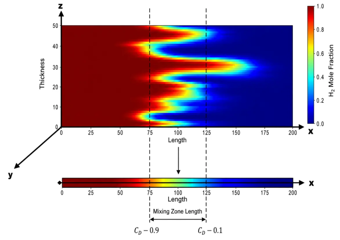
Figure 1. 1D representation for a 2D XZ simulation to calculate mixing zone length with gravity effects.
3.2. Distinguishing Fluid Flow Mechanisms Through Permeable Media
Three major mechanisms that control fluid flow are gravity segregation (i.e., the density difference between the fluid pair), dispersive mixing, and heterogeneity-driven channeling.
3.3. Gravity Segregation Effects
When a denser fluid displaces a lighter one, gravity segregation can significantly accelerate breakthrough in otherwise homogeneous reservoirs. In such settings, gravity becomes the dominant displacement mechanism when permeability-driven channeling is minimal. Consequently, the vertical-to-horizontal permeability ratio becomes a key parameter for both miscible and immiscible displacements. The density contrast between the injected and resident gases further amplifies gravity-driven flow, making it essential to quantify and account for it in dispersion analysis.
To isolate the influence of gravity within the 2D stochastic model, we repeated the simulations with the domain oriented along the x–y plane, as shown in Figure 2. In these cases, the vertical-to-horizontal permeability ratio was defined as the ratio of permeability in the y-direction to that in the x-direction. Mole fraction profiles were then calculated along the y-axis to obtain a one-dimensional interpretation across the x-axis, rather than averaging mole fractions over the z-axis as in the original configuration.
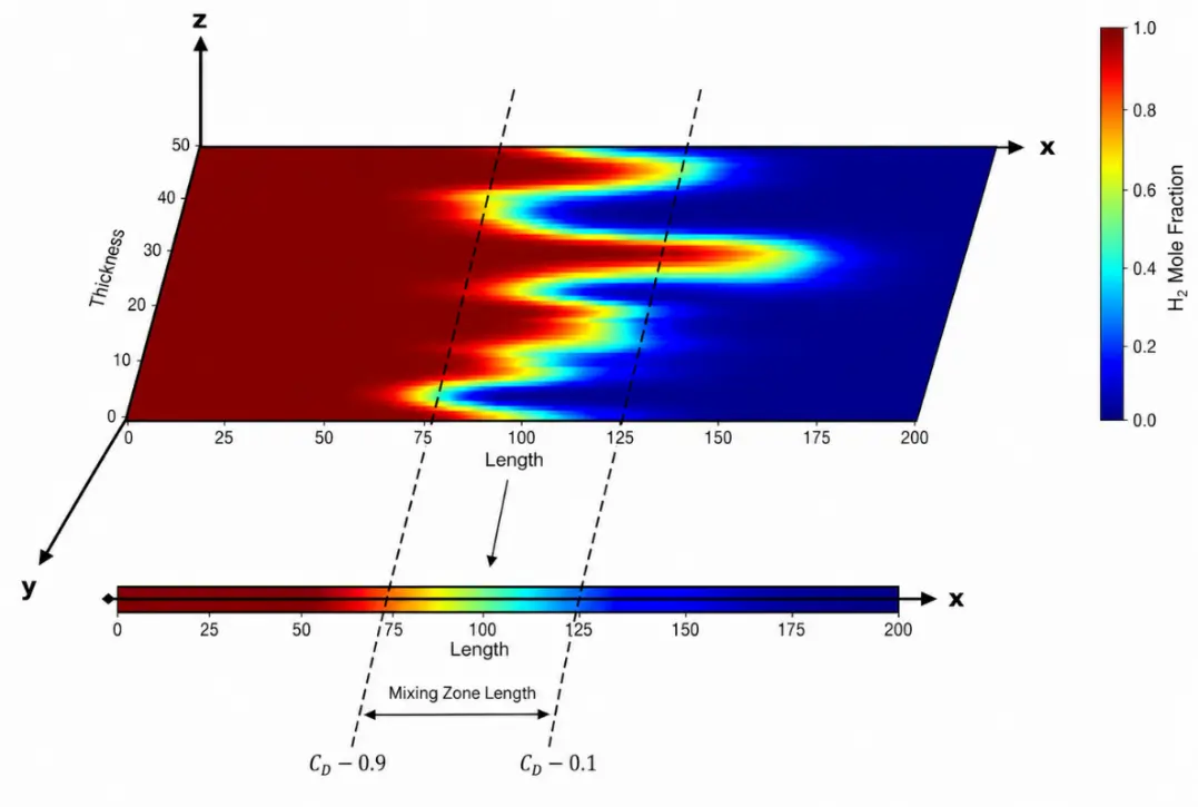
Figure 2. 1D representation for a 2D XY simulation to calculate mixing zone length excluding gravity effects.
3.4. Understanding of Mixing
To quantify mixing, we evaluate the mixing zone length for each layer of the model. As illustrated in Figure 3, mole fraction distributions are analyzed for every layer in the z-direction. The mixing zone length for a given layer is defined as the horizontal distance between the points where the dimensionless concentration CD equals 0.9 and 0.1, respectively. This length is calculated for each layer of the grid and then averaged over all layers.
The degree of mixing depends strongly on the heterogeneity present within each layer. This averaged value provides a measure of the overall mixing effect, which under most conditions is smaller in magnitude than the channeling effect. The average dimensionless mixing length difference is computed as:
|
```latexAverage \,Difference \left(∆{x}_{D}\right)= \frac{1}{n}\sum _{i=1}^{n}∆{x}_{{D}_{i}}``` |
(3) |
where n is the number of layers and $$∆{x}_{{D}_{i}}$$ is the dimensionless mixing length for the i-th layer.
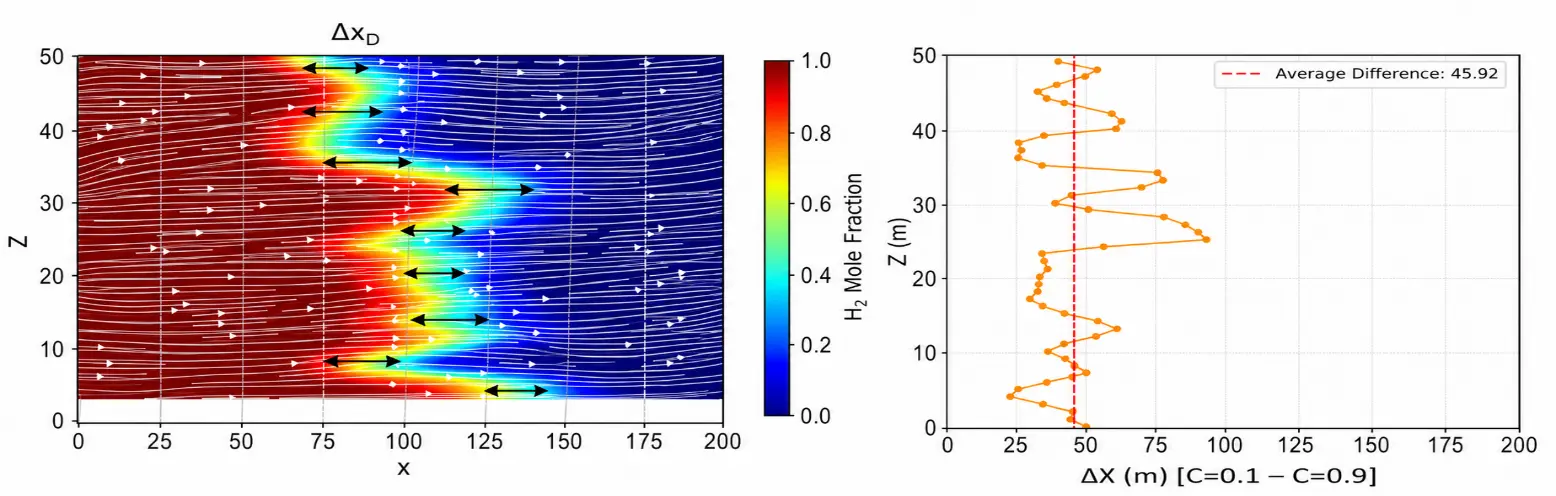
Figure 3. Representation for calculating mixing for the 2D simulations using the average difference. The arrows highlight the concentration differences between 0.9 and 0.1. The white lines indicate the streamlines.
3.5. Estimation of Local Dispersion
While local dispersion is a measurement of dispersion on the pore scale, the best approximation of that pore scale dispersion in simulations would be on a grid level. Therefore, an approximation can be made by solving the convective-diffusion equation for every grid block. This would be a proxy for local dispersion. A major caveat here is that local dispersion coefficients can be drastically different at different times. This is because during early times, the fluid flow is diffusion-dominated, and it transitions into channeling-dominated over time for a heterogeneous medium. For our study, however, we overcome this issue by performing our analysis at a fixed dimensionless time of 0.50.
|
```latex{D}_{local}= \frac{\frac{\partial C}{\partial t}+\stackrel{\to }{u}\cdot\nabla C}{{\nabla }^{2}C}``` |
(4) |
The dimensionless time (tD) is a ratio of the injected cumulative gas volume at reservoir conditions at a specific time to the volume of H2 needed to occupy the reservoir hydrocarbon pore volume. The equation for computing the dimensionless time is the following:
|
```latex{t}_{D}=\frac{{Vi}_{{\mathrm{H}}_{2}}}{\sum _{i=1}^{{n}_{b}}{V}_{pi}\left(1-{S}_{wi}\right)}``` |
(5) |
where $${Vi}_{{\mathrm{H}}_{2}}$$ is the cumulative volume of H2 injected at time t at reservoir conditions, nb is the number of gridblocks, Vpi is the pore volume of gridblock i, and Swi is the initial water saturation of gridblock i.
4. Analysis of a Single Point Injector Case
Estimation of a One-Dimensional Mixing Zone Length for a Multidimensional Model
To quantify the mixing zone length for a 2D XZ simulation when the injection is radially outward, and production is radially inward, we first draw the iso-concentration contours of 0.90 and 0.10. Mixing occurs where the concentration gradient is largest, between the contours. The elliptical shape of the plume is attributed to a combination of gravity and buoyancy effects. We then divided the plane into 360 evenly spaced rays (1 per degree) cast outwards from the well center. For each ray, the points of intersection with the 0.10 and 0.90 contours were determined, and the absolute difference in radial distance between these two points was computed as shown in Figure 4. The average of these differences across all rays was defined as the average mixing zone length (MZL) for that time step. This process was repeated for each simulation date to track the evolution of the MZL over time. Note that the cyclic endpoints in the simulation are distinct from the tD = 0.5 used during displacement cases. The mixing was computed at the end of each injection cycle, rather than after production. During injection, the concentration gradients become well-defined, whereas in the production cycle, the 0.9 contour disappears entirely, making it impossible to compute. This is also visually evident in the mole fraction snapshots, where the high-concentration zones present after injection largely vanish following production. The same process is repeated for 2D XY simulations to exclude gravity effects.
Dispersion behavior differs fundamentally between linear and radial flow regimes due to differences in velocity and heterogeneity, which become particularly important under cyclic injection–production. In linear flow regimes, flow occurs along relatively uniform, parallel streamlines. Under cyclic operation, the streamlines diverge and converge from the injector and producer. This creates significant velocity gradients. This repeated divergence–convergence cycle leads to significant changes in plume geometry every cycle.
Under cyclic injection–production, reversibility is assessed based on the change in mixing between the end of injection and after withdrawal. Echo dispersion isolates the irreversible component of mixing, while transmission dispersion captures both reversible and irreversible contributions. Therefore, the ratio of echo to transmission dispersivity provides a quantitative measure of irreversibility in the system, if boundary and numerical dispersion effects are minimized.
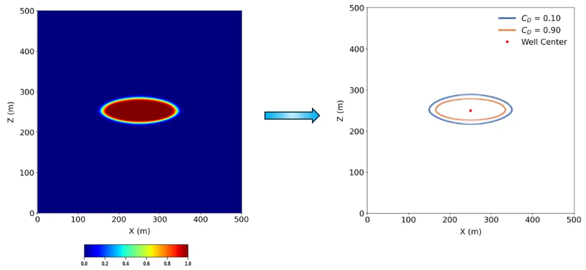
Figure 4. Representation for calculating the mixing zone length for the 2D simulations for a radial injection.
5. Simulation Setup and Results
5.1. Investigating Dispersive Behavior Through Heterogeneity and Vertical Permeability
5.1.1. Permeability Distribution
To estimate the impact of heterogeneity, we perform reservoir simulation on a 2D XZ cross-section stochastic model with dimensions of 200 m and 50 m in the x and z directions, respectively, and a grid size of 1 m × 1 m. All simulations were conducted using CMG-GEM, a compositional reservoir simulator developed by Computer Modelling Group. The simulations are performed using a structured Cartesian grid within the simulator, where the number of grids and the size of grids can be specified in each i, j, k direction. The permeability assignment is done to each grid via SLB-Petrel. Dykstra-Parsons Coefficient (VDP) and vertical-to-horizontal permeability ratios are varied to generate multiple fields. Autocorrelation lengths (λ) are kept at 120 m and 5 m in x and z, respectively. The initial reservoir pressure is set at 5 MPa, and a constant reservoir temperature of 60 °C is considered. Input longitudinal and transverse dispersivities are 1 cm and 0.1 cm, respectively. Pure H2 is the gas injected, and pure CH4 is the resident gas. The injection constraint was a maximum injection rate of 15 m3/day at reservoir conditions, and the producer constraint was set to the minimum bottomhole producer pressure of 5 MPa. The model is not intended to match a specific reservoir but rather to provide a generalized, physically realistic framework for analyzing dispersive transport. The input properties are tabulated in Table 1.
Table 1. Input properties used in the model.
|
Property |
Value |
|---|---|
|
Model dimensions (x, y, z) |
(200, 1, 50) |
|
Grid dimensions (x, y, z) |
(1, 1, 1) m |
|
Initial reservoir pressure |
5 MPa |
|
Reservoir temperature |
60 °C |
|
Porosity |
0.3 |
|
Mean |
100 mD |
|
Longitudinal dispersivity ($${\alpha }_{L}$$) |
1 cm |
|
Transverse dispersivity ($${\alpha }_{T}$$) |
0.1 cm |
|
Molecular diffusion |
Sigmund model (tortuosity = 1.4) |
|
Maximum injection rate on surface |
828.35 m3/day |
|
Producer minimum bottom hole pressure |
5000 kPa |
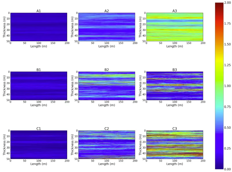
To investigate the relationship between permeability and dispersion, the 2D model was categorized into nine distinct cases, each defined by varying Dykstra-Parsons Coefficients (VDP) and vertical-to-horizontal permeability ratios (kz/kx). The VDP values for Cases A, B, and C were 0.3, 0.6, and 0.9, respectively. Each primary case was further subdivided into three scenarios based on average kz/kx ratios: Cases A1, A2, and A3 with an average kz/kx value of 0.1; Cases B1, B2, and B3 with an average kz/kx value of 0.5; and Cases C1, C2, and C3 with an average kz/kx value of 1.0. The kz/kx values within individual grid blocks in Case A1 do not uniformly equal 0.1; rather, their distribution averages to 0.1. The same logic applies to Cases B1, B2, B3, and C1, C2, C3. We generated a kz/kx map for every case and used the map to obtain vertical permeability. A detailed breakdown of these nine cases is presented in Table 2. The permeability distribution for the cases is shown in Figure 5. The autocorrelation lengths were 120 m in the horizontal direction and 5 m in the vertical direction.
Table 2. Description of the nine cases to understand the permeability distribution.
|
Cases |
Average Permeability (mD) in x-Direction |
Dykstra-Parsons Coefficient (VDP) |
Average Vertical to Horizontal Permeability Ratio (kz/kx) |
|---|---|---|---|
|
A1 |
100 mD |
0.3 |
0.1 |
|
A2 |
0.5 |
||
|
A3 |
1.0 |
||
|
B1 |
0.6 |
0.1 |
|
|
B2 |
0.5 |
||
|
B3 |
1.0 |
||
|
C1 |
0.9 |
0.1 |
|
|
C2 |
0.5 |
||
|
C3 |
1.0 |
5.1.2. Gas Mole Fraction Distribution
To understand the effect of dispersion, it is pertinent to observe the gas mole fraction distribution. The degree and the nature of the H2 displacement front spreading can be visually interpreted. Figure 6 shows the degree of mixing for all nine cases. Table 3 highlights the calculated Peclet Numbers for each case at tD = 0.5.
It is observed that both vertical permeability and heterogeneity contribute to deviations from the piston-like displacement expected in homogeneous systems, though in different ways. In reservoirs with lower kz/kx ratios, the flow remains dominated by the horizontal permeability distribution. As vertical permeability increases, the impact of gravity allows H2 to invade through multiple layers, especially in the top layers of the model. Moreover, the increase in the Dykstra-Parsons Coefficient (VDP) causes the flow to be more erratic and channeling-dominated due to preferential flow through high-permeability streaks.
From the effluent curves in Figure 7, the following can be deduced: The greater the heterogeneity is, the quicker the H2 breakthrough is. Once a breakthrough occurs, the effluent curve spreads out, showing a greater degree of mixing. At low heterogeneities, the H2 injected attempts to maintain its piston-like movement. Variations in vertical-to-horizontal permeability ratio (kz/kx) further influence plume distortion due to gravity segregation, contributing to asymmetry in the effluent response.
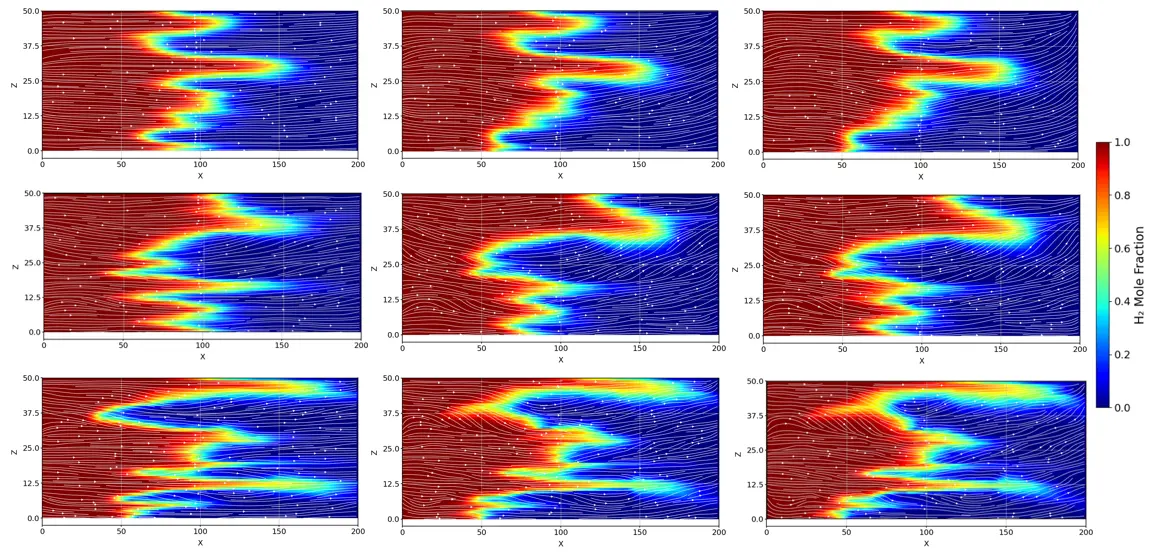
Figure 6. Gas mole fraction distribution as a function of increasing Dykstra-Parsons coefficient (top to bottom: 0.3, 0.6, and 0.9) and kz/kx (left to right: 0.1, 0.5, 1.0) at tD = 0.5.
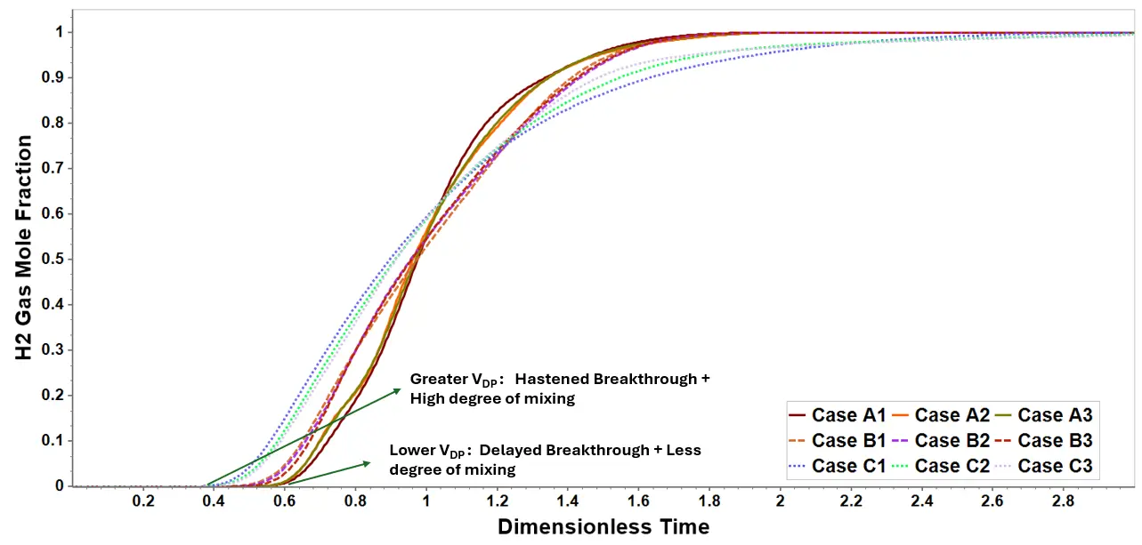
Table 3. Cases and corresponding Peclet Numbers and Dispersion Coefficient.
|
Cases |
Calculated Peclet Number |
Dispersion Coefficient (m2/Day) |
|---|---|---|
|
A1 |
50.69 |
1.032 |
|
A2 |
31.05 |
1.780 |
|
A3 |
28.51 |
1.953 |
|
B1 |
34.72 |
1.577 |
|
B2 |
20.22 |
2.816 |
|
B3 |
19.87 |
2.860 |
|
C1 |
15.08 |
3.821 |
|
C2 |
16.29 |
3.531 |
|
C3 |
16.29 |
3.531 |
Across the nine permeability cases, the calculated dispersion Coefficient values highlight dependence on both heterogeneity and anisotropy. Comparing these results with another CO2–CH4 study using the same setup, which employed the same permeability case framework, reveals clear differences between the CO2–CH4 and H2–CH4 systems [28]. The dispersion coefficients for H2–CH4 are of a larger magnitude (twice in some cases). This is due to a combination of buoyancy, where H2 rises due to gravity override, while CO2 tends to be gravitationally stable. Hence, the H2 plume gets distorted more quickly. The difference in density between H2 and CH4 is also higher than that between CH4 and CO2. H2 is also more mobile than CH4 and easily bypasses low-permeability zones under heterogeneity. Also, compared with the CO2–CH4 benchmark breakthrough curves, the H2–CH4 effluent curves exhibit stronger separation and do not overlap for the higher VDP cases.
5.2. Isolating Fluid Flow Mechanisms Through Permeable Media
5.2.1. Gravity
To better assess the gravity effects, all cases were run as XY cross-sections (areal simulations), as highlighted in Figure 2. The cases were similarly divided into three cases: A, B, and C, with VDP of 0.3, 0.6, and 0.9, respectively. However, the permeability ratio now refers to ky/kx instead of kz/kx.
Referring to Figure 8, in the cases excluding gravity, the displacement front remains horizontally oriented and more uniformly distributed across layers. For the same VDP, the visualizations are the same with changing permeability ratios. The displacement front shows greater channeling as heterogeneity increases, but without the exaggerated upward distortion seen in the gravity-included scenarios. Although not shown here, we do observe that in early times, the differences between gravity-included and excluded scenarios are minimal. Over time, buoyancy effects substantially dominate the concentration distribution.
Figure 9 shows the dC/dt snapshot at a tD of 0.50. This can help delineate some of the zones where the front is rapidly evolving. Light-colored regions (e.g., yellow and gray) represent zones experiencing the most rapid increase in H2 concentration, effectively delineating the moving front. In contrast, green or teal areas represent stagnant zones where the mole fraction has either stabilized due to complete saturation (H2 already displaced CH4) or has yet remained unaffected by injection. The dC/dt visualizations are not used to compute dispersion coefficients directly but are used to identify regions of compositional change.
The leading and the trailing edges have lower (or zero) dC/dt values, whereas the center of the mixing zone has the highest dC/dt values. This is because both the edges of the mixing zone have either already been completely saturated or are yet to be saturated with H2. In homogeneous systems, the front is comparatively continuous. As heterogeneity increases, the dC/dt field becomes fragmented and spread out. This fragmentation is, in fact, indicative of heterogeneous zones. Table 4 shows the local dispersion coefficient, while Table 5 shows the calculated Peclet Numbers.
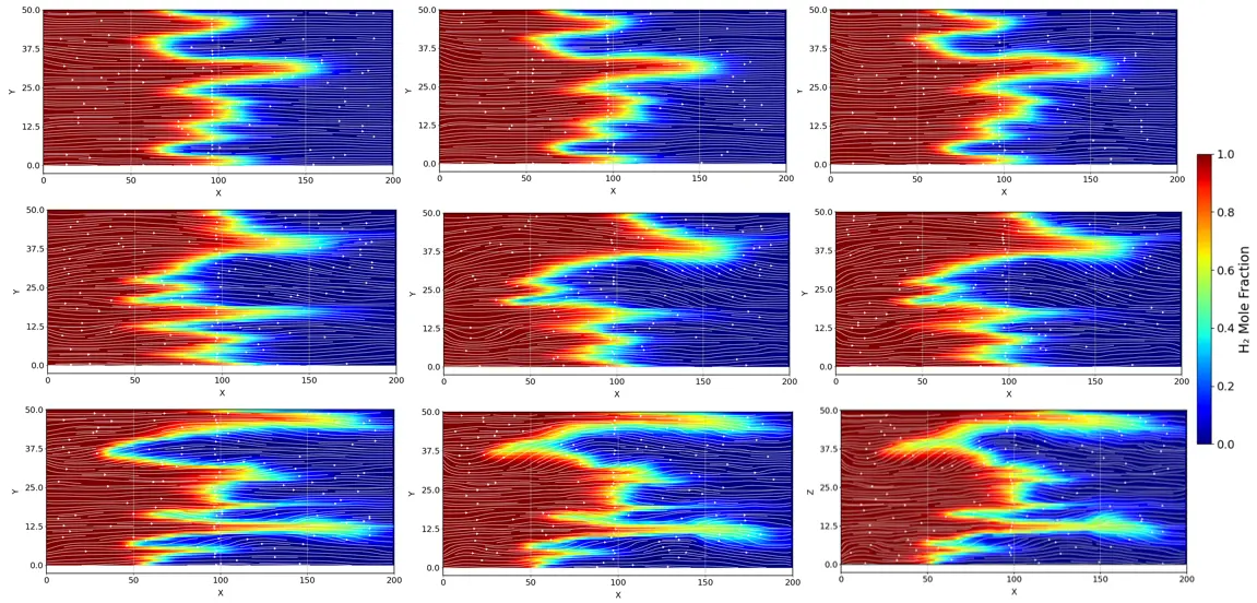
Figure 8. Gas mole fraction distribution as a function of increasing Dykstra-Parsons coefficient (top to bottom: 0.3, 0.6, and 0.9) and ky/kx (left to right: 0.1, 0.5, 1.0) at tD = 0.5, excluding gravity.
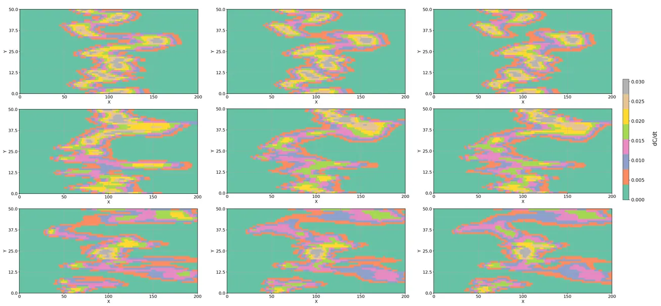
Figure 9. dC/dt as a function of increasing Dykstra-Parsons Coefficient (top to bottom: 0.3, 0.6, and 0.9) and ky/kx (left to right: 0.1, 0.5, 1.0) at tD = 0.5, excluding gravity.
For the gravity-free cases, we calculated the local dispersion coefficient for all nine scenarios on a grid-by-grid basis, then averaged these values only within the mixing zone to obtain the mean local dispersion coefficient at a dimensionless time of 0.50. Based on these results and comparison with previous cases, we draw the following conclusions:
-
Local dispersion is significantly lower than transmissive dispersion, and the latter is typically derived from averaging,
-
The mean local dispersion coefficient decreases as heterogeneity increases. When compared with overall dispersion coefficient trends, this suggests that channeling plays a more dominant role in heterogeneous media in explaining the overall dispersion coefficient.
Table 4. Cases excluding gravity and corresponding local dispersion coefficient.
|
Cases |
Local Dispersion Coefficient (m2/Day) |
|---|---|
|
A1 |
0.6065 |
|
A2 |
0.6714 |
|
A3 |
0.6674 |
|
B1 |
0.4588 |
|
B2 |
0.4731 |
|
B3 |
0.4923 |
|
C1 |
0.2628 |
|
C2 |
0.3366 |
|
C3 |
0.3372 |
Table 5. Cases excluding gravity and corresponding Peclet Numbers and Dispersion coefficient.
|
Cases (No Gravity Is Modeled) |
Calculated Peclet Number |
Dispersion Coefficient (m2/Day) |
|---|---|---|
|
A1 |
49.31 |
1.216 |
|
A2 |
42.11 |
1.424 |
|
A3 |
41.06 |
1.461 |
|
B1 |
35.53 |
1.688 |
|
B2 |
25.76 |
2.328 |
|
B3 |
24.77 |
2.422 |
|
C1 |
15.08 |
3.977 |
|
C2 |
16.82 |
3.567 |
|
C3 |
17.37 |
3.453 |
5.2.2. Understanding of Mixing
To understand the effects of mixing, we find the mixing zone length across each layer. The degree of mixing is a function of heterogeneity across each layer. We then calculate the average mixing zone length from all the layers. The average difference calculated in Figure 10 gives a measure of the mixing effect and is always less than the channeling effect.
We also make a comparison between the cases to calculate the mixing zone length with and without gravity effects. From the values in Table 6, we can deduce that the mixing averages across each layer thickness are directly proportional to the heterogeneity. The more heterogeneous a model is, the more mixing is perceived. For the ranges of vertical permeability studied, this mixing zone does not vary. This leads to the conclusion that, for the ranges of vertical permeability studied, mixing is a function only of permeability in the direction of flow.
Table 6. Cases excluding gravity effects and corresponding Peclet Numbers.
|
Cases |
Mixing Zone Contribution Including Gravity for H2–CH4 |
Mixing Zone Contribution Excluding Gravity (EG) for H2–CH4 |
|---|---|---|
|
A1 |
45.92 |
46.84 |
|
A2 |
47.64 |
48.64 |
|
A3 |
48.30 |
49.34 |
|
B1 |
54.75 |
55.10 |
|
B2 |
51.78 |
53.90 |
|
B3 |
51.72 |
53.84 |
|
C1 |
68.30 |
74.12 |
|
C2 |
71.28 |
72.26 |
|
C3 |
68.10 |
74.36 |
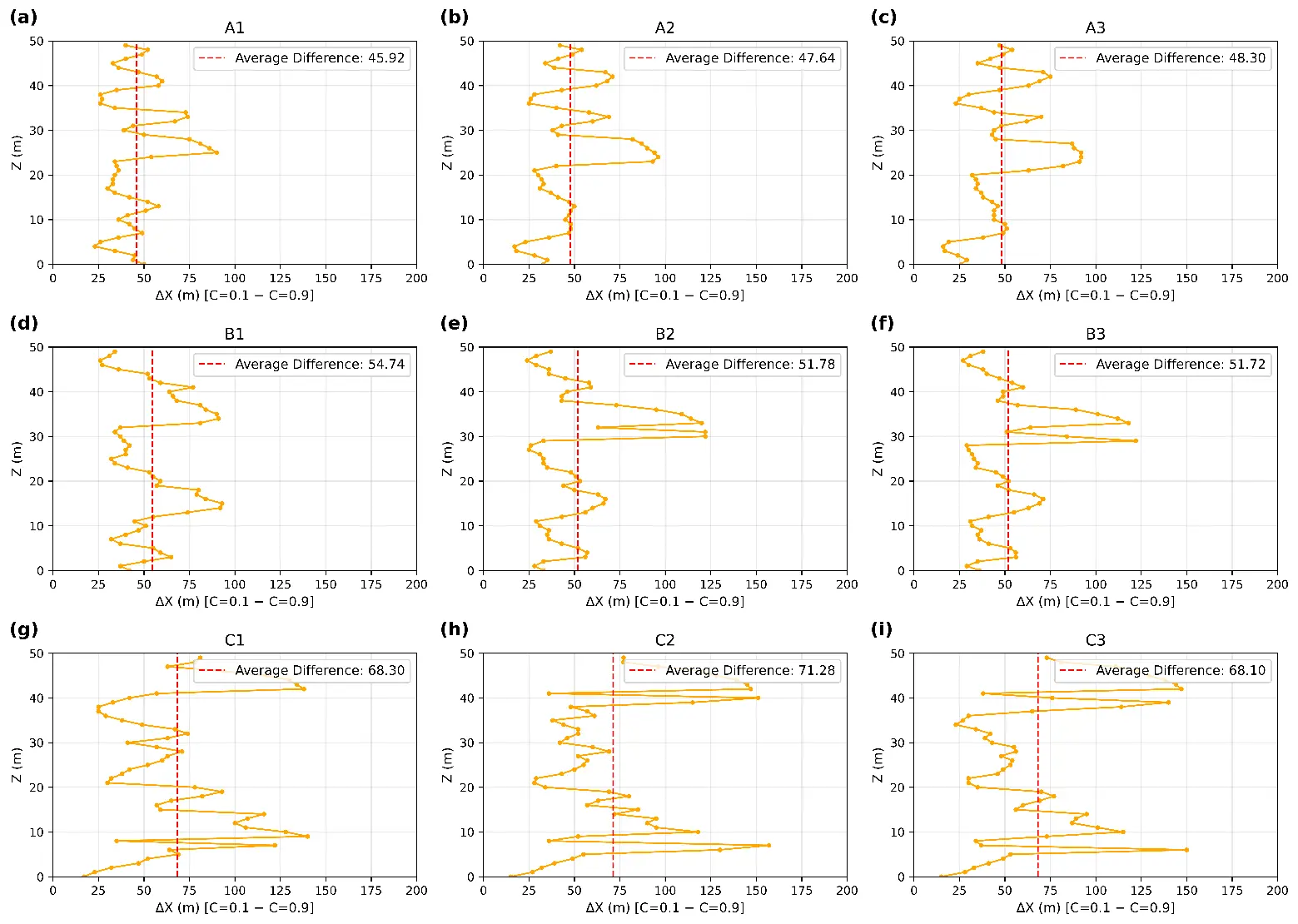
Figure 10. Calculation of mixing as a function of increasing Dykstra-Parsons Coefficient (top to bottom: 0.3, 0.6, and 0.9) and kz/kx (left to right: 0.1, 0.5, 1.0) at tD = 0.5, excluding gravity. Subfigures correspond to individual cases: (a) A1; (b) A2; (c) A3; (d) B1; (e) B2; (f) B3; (g) C1; (h) C2; and (i) C3. The dashed red line indicates the average mixing zone thickness for each case.
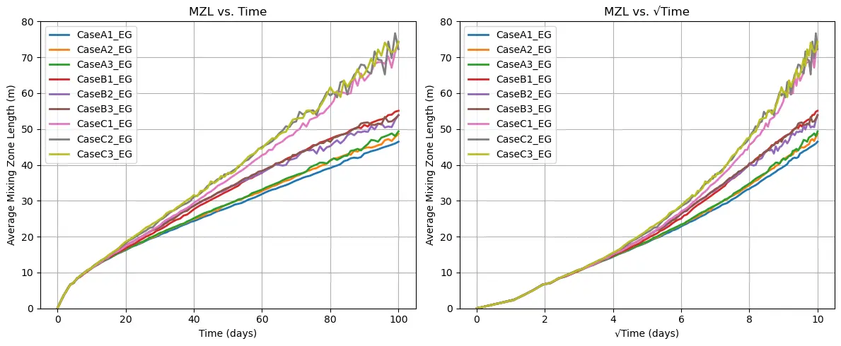
Further, the mixing length growth with time was also calculated for all times until the producer breakthrough within the model. It may be noted that greater heterogeneity is a significant contributor to the calculated mixing zone lengths than the vertical permeability itself. There are small fluctuations, but the mixing zone length is proportional to time as seen in Figure 11.
5.3. Investigating Dispersive Behavior Through Heterogeneity and Autocorrelation Lengths
Permeability fields in the x-direction were generated for varying amounts of heterogeneity, expressed using VDP and dimensionless autocorrelation lengths (λR). We parameterize heterogeneity by (i) the permeability distribution, which is the lognormal variance represented by the Dykstra-Parsons Coefficient, and (ii) a specified spatial distribution of the permeability distribution, which is represented by the autocorrelation length (λ). Therefore, with increasing autocorrelation length, the permeability distribution changes from random, coarse values of permeability to a layered distribution, which increases channeling.
The vertical permeability and the horizontal permeability were kept equal. Spatial correlation in the direction transverse to flow was held constant at 0.1 times the thickness. Figure 12 shows the permeability distribution for this case, and Figure 13 visualizes the gas mole fractions. Similar studies have been performed for gas-gas displacements [29].
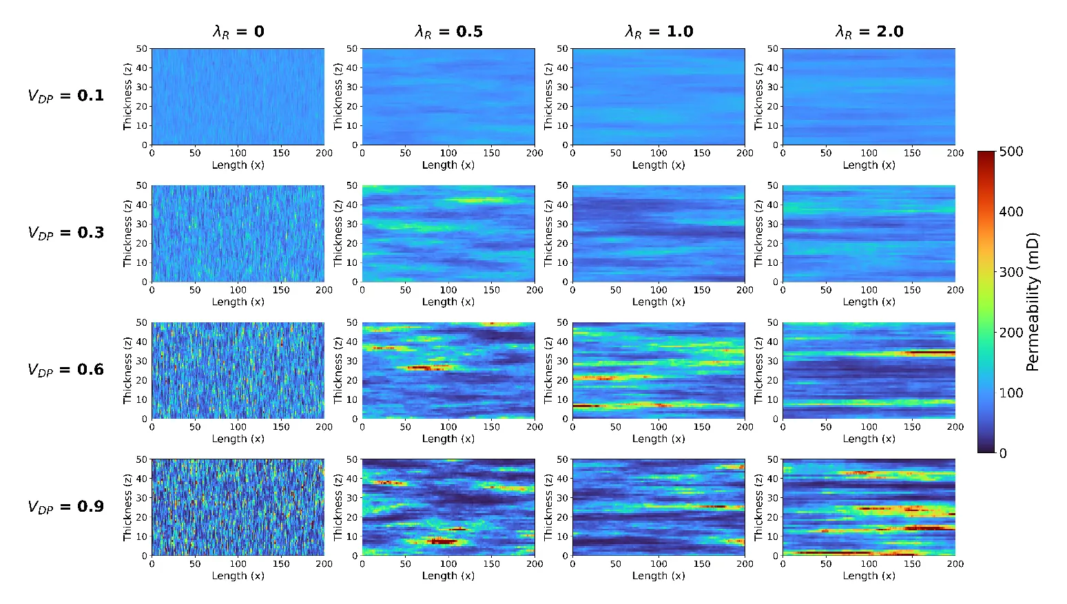
Figure 12. Permeability (in md) distribution for different VDP values and dimensionless autocorrelation lengths.
In the top row (VDP = 0.1), the permeability field is nearly homogeneous. As a result, the front propagates uniformly, and the influence of gravity dominates the flow of H2. This is evidenced by the vertical asymmetry in the H2 front, with preferential advancement in the upper layers due to the buoyant nature of hydrogen. The flow is diffusion-dominated, and minimal lateral deviation is observed across λR, as the spatial distribution has little impact in the absence of underlying heterogeneity.
As VDP increases (progressing downward), the heterogeneity in permeability intensifies, introducing significant variability in flow velocity across the domain. This enhanced heterogeneity promotes local velocity contrasts, which in turn distort the advancing plume. The interface becomes irregular and complex, signaling the onset of early-stage channeling, especially at intermediate and high VDP values.
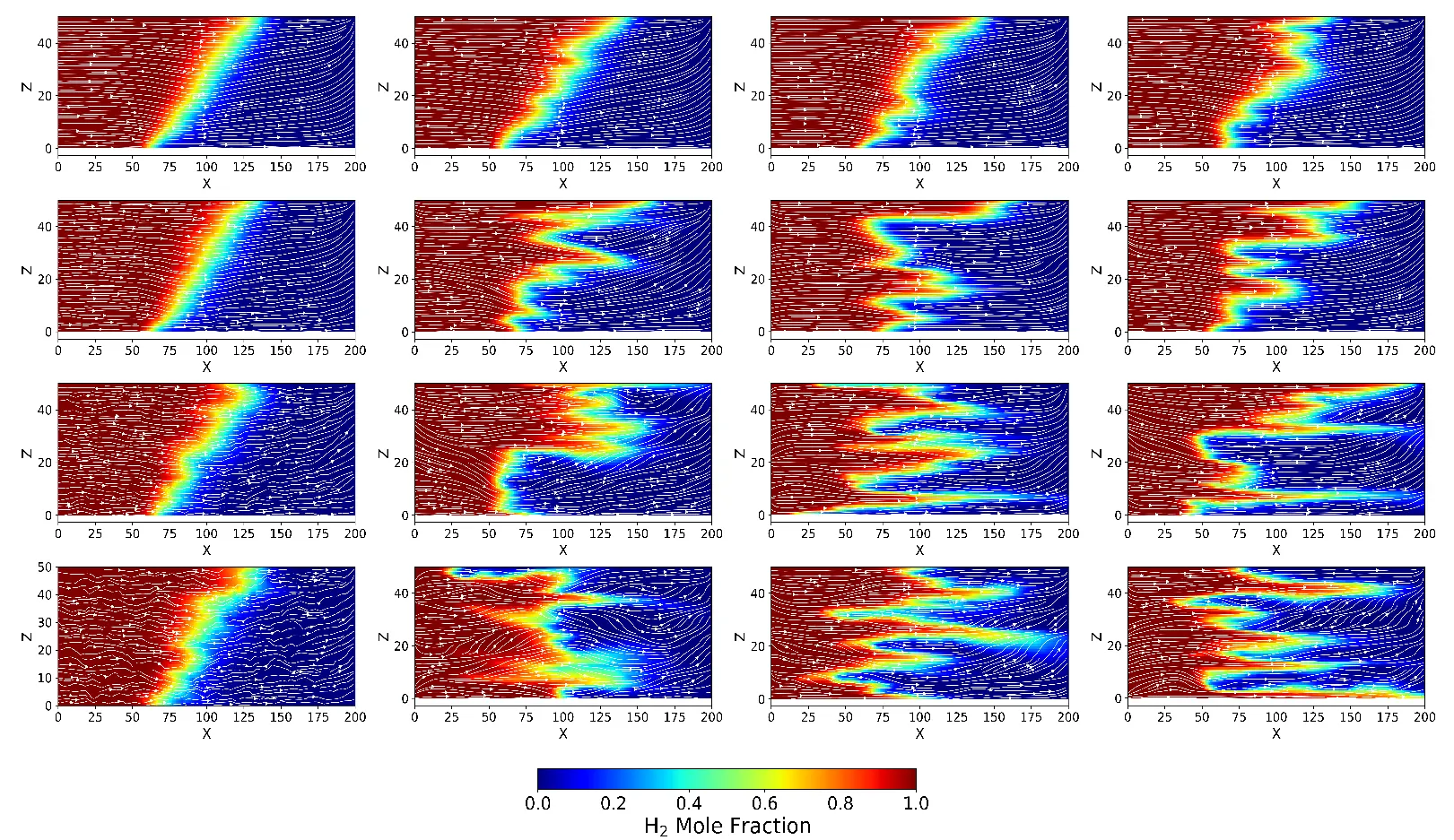
Figure 13. Gas Mole Fraction for different VDP and dimensionless autocorrelation at a dimensionless time tD = 0.5.
Simultaneously, increasing λR (left to right) imposes spatial continuity to the permeability distribution. While low λR cases (first column) are dominated by random, unstructured heterogeneity, higher λR values generate more stratified, layered systems. This layering aligns permeability in horizontal bands and the high-permeability conduits pathways that preferentially guide the flow. As a result, the H2 front becomes increasingly anisotropic, displaying elongated tongues and narrow fingers aligned with the direction of correlation.
At the bottom-right corner (high VDP and high λR), these effects culminate in the most pronounced channeling behavior. The flow is no longer governed solely by gravity or molecular dispersion; instead, it becomes structurally constrained, with minimal transverse mixing and maximum front distortion. This regime represents a shift from Fickian dispersion to mechanically induced anisotropic transport, driven by the reservoir’s intrinsic architecture.
Between the extremes of autocorrelation length, there is a concept of critical range λRc. For each VDP, there is a specific value of dimensionless autocorrelation length after which the displacement indicates channeling. Below λRc, the overall effect is dispersive, and above λRc, the overall behavior is both dispersive and channeling. Because the transition between the two zones is gradual, the line of λRc is qualitative. Figure 14 highlights the relation between λR and VDP. The green curve here shows the λRc and helps in differentiating the channeling and dispersive regions. The transition between these regions is gradual; therefore, the placement of the λRc line is determined based on qualitative judgment.
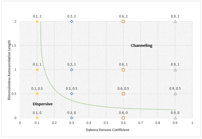
Figure 14. Plot of dimensionless autocorrelation lengths versus Dykstra-Parsons Coefficient (VDP) delineating dispersive versus channeling zones. Markers denote heterogeneity levels characterized by VDP: × (0.1), ◇ (0.3), □ (0.6), and △ (0.9).
6. Analysis of Radial Injection and Production
To study dispersive hydrogen transport under cyclic injection and withdrawal, a 2D simulation model was developed using a homogeneous porous medium initially saturated with methane (CH4). A single well located at the center of the domain acted alternately as an injector and a producer. The simulation consisted of five cycles, each comprising 180 days of H2 injection followed by 180 days of production, totaling approximately 5 years. No shut-in period was imposed between the injection and production phases. Table 7 highlights the reservoir properties for this case.
The injected hydrogen can be conceptualized as a pulse or signal introduced into the reservoir. In a perfectly reversible system, such a signal could be “rewound”: the flow direction is reversed, and the hydrogen would retrace its path back to the well in the same amount of time, resulting in identical concentration snapshots during injection and production. However, as evident from Figure 15 and Figure 16, the plume does not fully deconstruct, and a remnant concentration halo persists around the well. This mismatch indicates irreversible mixing driven by velocity and pressure differences. In theory, reversibility would also imply that any mixed component could become unmixed upon reversal, but in practice, true mixing processes (e.g., diffusion or mechanical dispersion) are difficult to reverse.
Table 7. Reservoir Properties to study the radial injection dispersion.
|
Property |
Value |
|---|---|
|
No. of Gridblocks in each direction |
501 × 1 × 501 |
|
Gridblock Dimensions |
1 m × 1 m × 1 m |
|
Porosity |
0.3 |
|
Permeability |
100 mD (Average) |
|
Diffusion coefficient |
0.01365 m2/day |
|
Input longitudinal dispersivity |
0.02 m |
|
Initial pressure |
5000 kPa |
|
Constraints: |
|
|
Injection Constraint (Max BHF) |
15 m3/day |
|
Producer Constraint (Max BHF) |
15 m3/day |
In the absence of gravity, the H2 plume spreads symmetrically and leads to a circular front during injection and a collapsed front of the mixed zone during production around the wellbore, as shown in Figure 15. Equal volumes of gas are being injected and produced each cycle. The injected volume consists solely of H2, while the produced volume contains both pure H2 and the mixed H2+CH4 phase. Over successive cycles, this creates a more dispersed field and a more prominent mixing zone.
The inclusion of gravity modifies this geometry. Both dispersion and buoyancy create the modified oval shape geometry of the plume, which is distorted over subsequent cycles as gravity becomes increasingly significant. Figure 16 shows the H2 gas mole fraction with the inclusion of gravity. This gravity-driven override begins to compete with dispersive forces, shifting the center of mass of the injected plume. During production, denser CH4 from the lower part of the domain is preferentially produced, leaving behind a more stratified H2-rich zone at the top. Therefore, injection schemes that account for the gravity segregation of H2 become pertinent.
In Table 8, we observe that without gravity, the MZL is longer than with gravity. In the absence of gravity, the displacement front expands radially in all directions, allowing dispersion to act uniformly and resulting in broader transition zones between the resident and injected gases. However, with gravity, H2 rises to the top quickly, leading to the collapse of the circular plume to a collapsed vertical plume. The portion of this plume near the well exhibits minimal mixing, while only the distal edge undergoes significant dispersion. This asymmetry leads to a reduced average MZL, as most of the domain remains sharply stratified with little contribution to the mixing zone.
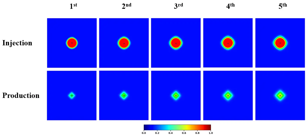
Figure 15. Gas Mole Fraction at the end of each injection (top) and the end of each production (bottom) from left to right, excluding gravity effects.
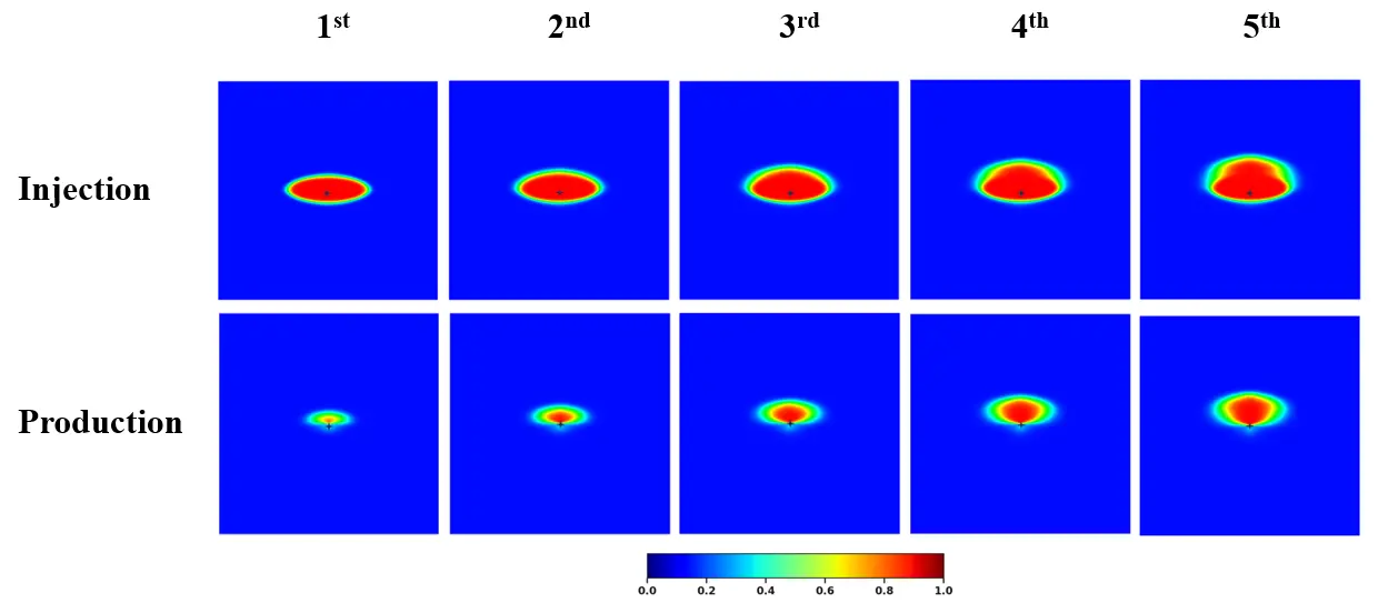
Figure 16. Gas Mole Fraction at the end of each injection (top) and the end of each production (bottom) from left to right, including gravity effects.
Table 8. MZL calculation at the end of each injection.
|
Injection Number |
MZL with Gravity (m) |
MZL without Gravity (m) |
|---|---|---|
|
1st |
11.56 |
12.85 |
|
2nd |
14.35 |
16.18 |
|
3rd |
15.96 |
19.05 |
|
4th |
17.21 |
21.48 |
|
5th |
18.46 |
23.61 |
Impact of Heterogeneity
The same simulations were performed again within a heterogeneous medium under similar conditions. The heterogeneity patterns are shown in Figure 17.
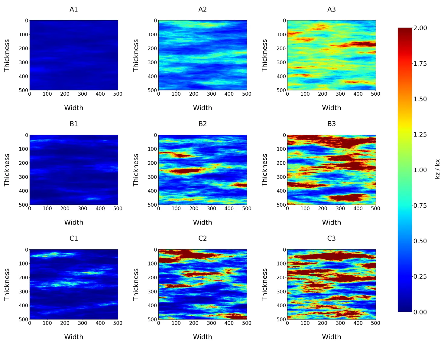
Figure 17. Permeability field distribution for radial MZL study with varying Dykstra-Parsons Coefficient (VDP) = 0.3, 0.6, and 0.9 (top to bottom) and kz/kx = 0.1, 0.5, and 1.0 (left to right).
In a heterogeneous medium with a single injector source, dispersion is a combination of both echo and transmission dispersion. The higher the kz/kx is, the stronger the viscous force, and higher vertical propagation of H2 is observed. The contours from Figure 18, despite being irregularly shaped, exhibit a certain degree of symmetry, which becomes distorted as both heterogeneity and vertical permeability increase. As heterogeneity increases, the plume shapes get horizontally distorted, and the plume deviation across permeability streaks becomes more apparent.
The average width of the mixing zone between the two iso-concentration contours does not substantially change as seen in Table 9, implying that while the plume geometry is sensitive to heterogeneity under balanced force conditions, dispersion-driven mixing remains almost equal. The differences in the MZL between all the cases (given the cell size is 1 m by 1 m) are negligible. This indicates that while heterogeneity significantly affects front shape and breakthrough patterns, its influence on the averaged mixing zone length (MZL) remains modest in those heterogeneous systems.
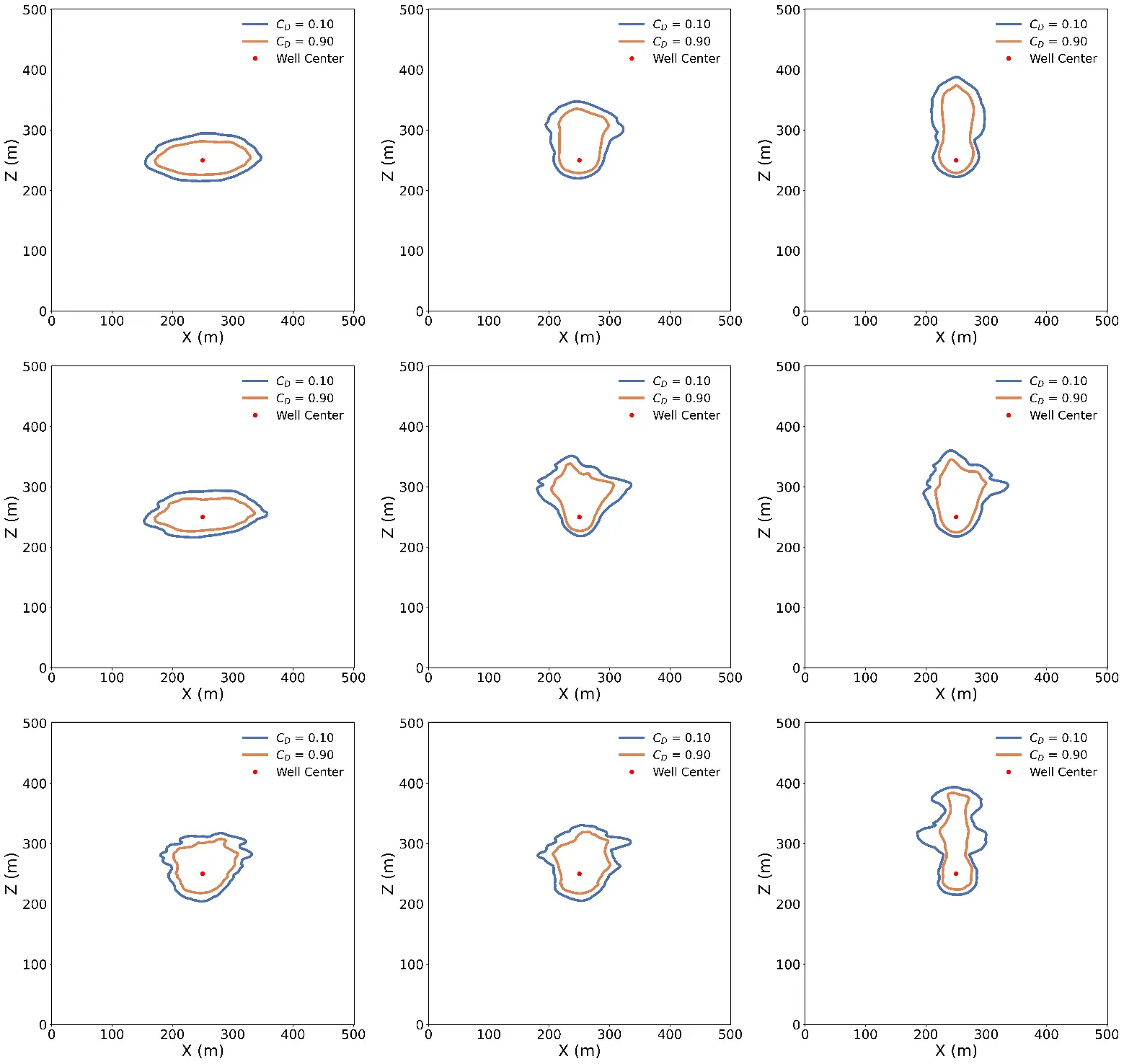
Figure 18. Permeability Distribution showing the contours with CD = 0.90 and CD = 0.10 for varying Dykstra-Parsons Coefficient (VDP) = 0.3, 0.6, and 0.9 (top to bottom) and kz/kx = 0.1, 0.5, and 1.0 (left to right).
Table 9. MZL calculation at the end of the first injection by averaging the mixing zone lengths.
|
Cases |
Average MZL by Averaging (m) |
|---|---|
|
A1 |
13.94 |
|
A2 |
12.79 |
|
A3 |
13.19 |
|
B1 |
14.09 |
|
B2 |
13.74 |
|
B3 |
13.62 |
|
C1 |
13.56 |
|
C2 |
13.92 |
|
C3 |
12.89 |
Due to the continuous injection and production phases in our cyclic operation, the post-production concentration fields do not exhibit a sharp, well-defined isosurface front with CD = 0.9. This makes the traditional method of calculating differences between 0.9 and 0.1 concentrations, commonly used in 1D dispersion analysis, impractical for our case. Therefore, we adopt a variance-based approach to determine the mixing zone length, which is widely used in statistical analyses of irregular dispersive plumes. In this method, the spatial variance of the front location is calculated after applying a concentration filter (0.1 < CD < 0.9) to isolate the transition zone between injected and resident gases. The resulting standard deviation of the front position is then converted to an equivalent mixing zone length using the scaling from the analytical solution of the convective–diffusive equation. This formulation naturally accounts for the irregular geometry of the dispersive front, making it suitable for both heterogeneous and gravity-influenced systems. We apply this same procedure to two key snapshots in each cycle: (1) at the end of the injection phase, where the derived dispersion coefficients represents the transmission dispersion (total reversible and irreversible spreading), and (2) at the end of the production phase, where the derived dispersion coefficient represents the echo dispersion (irreversible spreading retained after reversal of flow). The ratio of echo to transmission dispersion in Table 10 serves as a dimensionless measure of the degree of irreversibility in the system.
In the 2D simulations, the irreversibility of the plume appears to correlate with the directional spread of the plume. The more vertically or horizontally the plume travels in comparison to radially outward, the more reversible it becomes. The more radially H2 spreads, i.e., cases with intermediate heterogeneity and limited verticality, the more irreversible it becomes. Although in some cases, the variance-based definition of mixing zone length yields echo values greater than transmission values, this does not imply increased physical spreading during production. This reflects the redistribution and fragmentation of the plume after flow reversal, which increases the spatial variance of the concentration field.
Table 10. Echo and transmission mixing zone lengths and irreversibility ratio for cyclic radial injection-production.
|
Case |
MZL (Transmission) |
MZL (Echo) |
Ratio of Irreversibility (MZLecho/MZLtransmission) |
|---|---|---|---|
|
A1 |
19.62 |
11.09 |
0.320 |
|
A2 |
22.99 |
29.27 |
1.677 |
|
A3 |
36.16 |
33.62 |
0.864 |
|
B1 |
20.17 |
12.06 |
0.358 |
|
B2 |
23.02 |
32.96 |
2.050 |
|
B3 |
24.80 |
33.92 |
1.871 |
|
C1 |
18.48 |
18.01 |
0.949 |
|
C2 |
18.99 |
25.00 |
1.737 |
|
C3 |
37.28 |
33.64 |
0.814 |
7. Summary and Conclusions
-
-
We developed a method to extract effective dispersion Coefficients from multidimensional mole fraction fields by mapping them to one-dimensional mixing zone lengths. This procedure allows consistent comparison across scales and heterogeneities.
-
-
Increasing Dykstra Parsons Coefficients intensifies channeling, which causes earlier hydrogen breakthrough and greater plume distortion. Heterogeneity exerts a stronger influence on mixing zone growth than vertical permeability within the studied ranges. The effective dispersion coefficient increases from approximately 1.03 to 3.5 m2/day as the Dykstra–Parsons coefficient increases from 0.3 to 0.9.
-
-
Gravity segregation significantly alters displacement behavior, producing asymmetric plumes and reducing effective mixing zone lengths compared to gravity-free systems.
-
-
Local dispersion coefficients are consistently smaller than transmission values and range from 0.26 to 0.67 m2/day, indicating that apparent large-scale spreading is largely controlled by channeling and convective transport rather than localized mixing.
-
-
Cyclic injection-production simulations reveal irreversible dispersion. The ratio of echo to transmission dispersion highlights that only part of the spreading is reversible, which has direct implications for storage efficiency and purity of withdrawn hydrogen. The ratios range from 0.32 to 2.05.
These results emphasize that storage performance in depleted reservoirs cannot be evaluated accurately with homogeneous assumptions or molecular diffusion models. Accurate assessment requires explicit consideration of heterogeneity, anisotropy, and buoyancy. The effluent curves can be directly used to assess practical storage performances. The effective dispersion coefficient directly impacts storage performance by controlling hydrogen purity during withdrawal, as earlier breakthrough reduces produced gas quality, and working gas recovery, as increased dispersion leads to larger mixing zones and reduced recoverable hydrogen volumes. Therefore, higher dispersion coefficients correspond to lower recovery efficiency and increased contamination by cushion gas.
8. Terminology
Diffusion: Diffusion is the movement of molecules from regions of high concentration to low concentration due to random molecular motion, driven by a concentration gradient. It does not require bulk flow or external forces and occurs independently of velocity.
Dispersion: Dispersion is the process by which fluid spreads in a porous medium due to velocity variations caused by heterogeneities in the pore structure and flow paths. This leads to a broader distribution of the solute or gas, resulting in a concentration range between 0 and 1, as the solute mixes with the surrounding fluid.
Mixing: Mixing in porous media is the process by which a fluid spreads and homogenizes due to the combined effects of molecular diffusion and mechanical dispersion, leading to a gradual transition in concentration.
Apparent Mixing: Apparent mixing refers to the combined spreading, which occurs not only due to dispersion and mixing but also because of additional factors such as gravity and solubility. These factors alter the behavior of the dispersed field, making it more complex than what would be expected from mixing alone.
Channeling: Channeling is the process by which a fluid preferentially flows through high-permeability pathways in a porous medium, leading to a situation where the concentration at all points is either 0 or 1, with large portions of the medium bypassed. This results in an uneven distribution of fluid.
Echo Dispersion: Echo Dispersion involves understanding of dispersion during the reversal of fluid flow and observations made at the source of injection. Therefore, echo dispersion captures the irreversible portion of dispersion by canceling out reversible spreading.
Transmission Dispersion: Transmission Dispersion is the effective spread during fluid flow and involves no fluid flow reversal.
Local Dispersion: It reflects intrinsic mixing at a point due to small-scale velocity and must be independent of channeling and gravity effects.
9. Nomenclature
The symbols and abbrevations used in this study are summarized in Table 11.
Table 11. Nomenclature used in this study.
|
Symbol |
Description |
Units |
|---|---|---|
|
Roman Symbols |
||
|
C |
Concentration |
- |
|
Dij |
Binary Diffusion Coefficients |
m2/day |
|
DL |
Dispersion Coefficient |
m2/day |
|
Dmol |
Molecular Diffusion Coefficient |
m2/day |
|
H |
Domain height |
m |
|
J |
Diffusive Flux |
mol m2/day |
|
kx |
Absolute permeability in the x-direction |
mD |
|
kz |
Absolute permeability in the z-direction |
mD |
|
L |
Domain length |
m |
|
Mi |
Molecular weight of component i |
- |
|
nb |
Number of grid blocks |
- |
|
Npe |
Peclet Number |
- |
|
R |
Universal gas constant |
J/K/mol |
|
Sw |
Mobile water saturation |
- |
|
Swi |
Initial water saturation |
- |
|
Swr |
Residual water saturation |
- |
|
T |
Temperature |
°C |
|
u |
Darcy velocity |
m/day |
|
vci |
Molar volume of component i in the gas phase |
m3/mol |
|
yi |
Molar fraction of component i in the gas phase |
- |
|
VDP |
Dykstra Parsons Coefficient |
- |
|
Greek Symbols |
||
|
μ |
Viscosity |
cP |
|
ρo |
Molar Density |
mol/m3 |
|
ρr |
Reduced Molar Density |
- |
|
σij |
Lennard-Jones parameter between components i and j |
kJ/mol |
|
Ωij |
Collision integral between components i and j |
- |
|
τ |
Tortuosity |
- |
|
Dimensionless Groups |
||
|
xD |
Dimensionless Distance |
- |
|
tD |
Dimensionless Time |
- |
|
λR |
Dimensionless autocorrelation length |
- |
|
λRc |
Dimensionless critical autocorrelation length |
- |
|
Abbreviations |
||
|
BHP |
Bottom Hole Pressure |
kPa |
|
MZL |
Mixing Zone Length |
m |
|
PVI |
Pore Volume Injected |
m3 |
Acknowledgments
The authors thank the Computer Modeling Group and SLB for providing access to their software.
Author Contributions
Conceptualization, K.M., M.D., B.R.B.F., L.W.L.; Methodology, K.M., M.D., B.R.B.F., L.W.L.; Software, M.D.; Validation, K.M., M.D., L.W.L., B.R.B.F., K.S.; Formal Analysis, B.R.B.F., K.S.; Investigation, K.M.; Resources, M.D., L.W.L. and K.S.; Data Curation, K.M.; Writing—Original Draft Preparation, K.M.; Writing—Review & Editing, B.R.B.F., M.D., L.W.L. and K.S.; Visualization, K.M.; Supervision, M.D., L.W.L. and K.S.; Project Administration, M.D.; Funding Acquisition, M.D., K.S.
Ethics Statement
Not applicable.
Informed Consent Statement
Not applicable.
Data Availability Statement
The data and input used in this study are available from the corresponding author upon request.
Funding
This research received no external funding.
Declaration of Competing Interest
The authors declare that they have no known competing financial interests or personal relationships that could have appeared to influence the work reported in this paper.
References
- Heinemann N, Alcalde J, Miocic JM, Hangx SJT, Kallmeyer J, Ostertag-Henning C, et al. Enabling large-scale hydrogen storage in porous media: The scientific challenges. Energy Environ. Sci. 2021, 14, 853–864. DOI:10.1039/d0ee03536j [Google Scholar]
- Miocic J, Heinemann N, Edlmann K, Scafidi J, Molaei F, Alcalde J. Underground hydrogen storage: A review. Geol. Soc. Lond. Spec. Publ. 2023, 528, 73–86. DOI:10.1144/SP528-2022-88 [Google Scholar]
- Wolf E. Large-Scale Hydrogen Energy Storage. In Electrochemical Energy Storage for Renewable Sources and Grid Balancing; Elsevier: Amsterdam, The Netherlands, 2015. DOI:10.1016/B978-0-444-62616-5.00009-7 [Google Scholar]
- Delshad M, Alhotan MM, Fernandes BRB, Umurzakov Y, Sepehrnoori K. Modeling flow and transport in saline aquifers and depleted hydrocarbon reservoirs for hydrogen energy storage. SPE J. 2023, 28, 2547–2565. DOI:10.2118/210351-PA [Google Scholar]
- Epelle EI, Obande W, Udourioh GA, Afolabi IC, Desongu KS, Orivri U, et al. Perspectives and prospects of underground hydrogen storage and natural hydrogen. Sustain. Energy Fuels 2022, 6, 3324–3343. DOI:10.1039/D2SE00618A [Google Scholar]
- Derakhshani R, Lankof L, GhasemiNejad A, Zarasvandi A, Amani Zarin MM, Zaresefat M. A Novel Sustainable Approach for Site Selection of Underground Hydrogen Storage in Poland Using Deep Learning. Energies 2024, 17, 3677. DOI:10.3390/en17153677 [Google Scholar]
- Derakhshani R, Lankof L, GhasemiNejad A, Zaresefat M. Artificial intelligence-driven assessment of salt caverns for underground hydrogen storage in Poland. Sci. Rep. 2024, 14, 14246. DOI:10.1038/s41598-024-64020-9 [Google Scholar]
- Bagchi C, Patwardhan SD, Iglauer S, Ben Mahmud H, Ali MFJ. A critical review on parameters affecting the feasibility of underground hydrogen storage. ACS Omega 2025, 10, 11658–11696. DOI:10.1021/acsomega.4c10442 [Google Scholar]
- Muhammed NS, Haq B, Al Shehri D, Al-Ahmed A, Rahman MM, Zaman E. A review on underground hydrogen storage: Insight into geological sites, influencing factors and future outlook. Energy Rep. 2022, 8, 461–499. DOI:10.1016/j.egyr.2021.12.002 [Google Scholar]
- Maniglio M, Pizzolato A, Panfili P, Cominelli A. A simple and practical approach to estimate dispersive mixing in underground hydrogen storage systems. In Proceedings of the SPE Annual Technical Conference and Exhibition, Houston, TX, USA, 3–5 October 2022. DOI:10.2118/210251-MS [Google Scholar]
- Marchbank S, Heinemann N, Wilkinson M, Edlmann K, Molnar IL. Field-scale dispersion between hydrogen and cushion gas in underground hydrogen storage and co-relation with gravity segregation. Int. J. Hydrogen Energy 2026, 223, 154166. DOI:10.1016/j.ijhydene.2026.154166 [Google Scholar]
- Akbari A, Maleki M, Kazemzadeh Y, Ranjbar A. Calculation of hydrogen dispersion in cushion gases using machine learning. Sci. Rep. 2025, 15, 13718. DOI:10.1038/s41598-025-98613-9 [Google Scholar]
- Saffman PG. A theory of dispersion in a porous medium. J. Fluid Mech. 1959, 6, 321–349. DOI:10.1017/S0022112059000672 [Google Scholar]
- Alhotan M, Jia C, Alsousy A, Delshad M, Sepehrnoori K. Impact of permeability heterogeneity coupled with well placement strategy on underground hydrogen storage reservoir simulation. In Proceedings of the SPE Middle East Oil and Gas Show, Manama, Bahrain, 19–21 February 2023. DOI:10.2118/213257-MS [Google Scholar]
- Mahadevan J, Lake LW, Johns RT. Estimation of true dispersivity in field scale permeable media. In Proceedings of the SPE/DOE Improved Oil Recovery Symposium, Tulsa, OK, USA, 13–17 April 2002. DOI:10.2118/75247-MS [Google Scholar]
- Li D, Emami-Meybodi H. Hydrogen mixing dynamics in depleted gas reservoirs. In Proceedings of the SPE Annual Technical Conference and Exhibition, New Orleans, LA, USA, 23–25 September 2024. DOI:10.2118/220710-MS [Google Scholar]
- Feldmann F, Hagemann B, Ganzer L, Panfilov M. Numerical simulation of hydrodynamic and gas mixing processes in underground hydrogen storage. Environ. Earth Sci. 2016, 75, 1165. DOI:10.1007/s12665-016-5948-z [Google Scholar]
- Kobeissi S, Ling NNA, Yang K, May EF, Johns ML. Dispersion of hydrogen in different potential cushion gases. Int. J. Hydrogen Energy 2024, 60, 940–948. DOI:10.1016/j.ijhydene.2024.02.151 [Google Scholar]
- Williams HA, Heinemann N, Molnar IL, de Mesquita L Veloso F, Gladding T, Rashwan TL. Hydrogen storage in depleted gas reservoirs with carbon dioxide as a cushion gas. Int. J. Hydrogen Energy 2025, 102, 1116–1129. DOI:10.1016/j.ijhydene.2024.12.371 [Google Scholar]
- Nazari F, Farajzadeh R, Shokri J, Vahabzadeh E, Lopez-Porfiri P, Perez-Page M, et al. Implications of non-ideal gas dispersion for underground hydrogen storage. Chem. Eng. J. 2025, 507, 160143. DOI:10.1016/j.cej.2025.160143 [Google Scholar]
- Yamada K, Delshad M, Lake LW, Sepehrnoori K, Fernandes BRB, Farajzadeh R. The role of miscible gas mixing on CO2-enhanced methane recovery. In Proceedings of the SPE Annual Technical Conference and Exhibition, New Orleans, LA, USA, 23–25 September 2024. DOI:10.2118/221024-MS [Google Scholar]
- Mawa K, Fernandes BRB, Delshad M, Lake LW, Farajzadeh R, Sepehrnoori K. Assessing the influence of reservoir heterogeneity on CO2 storage and dispersion patterns. In Proceedings of the SPE Conference at Oman Petroleum & Energy Show, Muscat, Oman, 12–14 May 2025. DOI:10.2118/224835-MS [Google Scholar]
- Hussain S, Machado MVB, Fernandes BRB, Delshad M, Sepehrnoori K. Geochemical analysis of underground hydrogen storage in a saline carbonate aquifer. In Proceedings of the Kuwait Oil & Gas Show, Kuwait City, Kuwait, 3–5 February 2026. DOI:10.2118/230925-MS [Google Scholar]
- Lake L, Johns RT, Rossen WR, Pope GA. Fundamentals of Enhanced Oil Recovery; Johns Hopkins University Press: Baltimore, MD, USA, 2014. [Google Scholar]
- Mamora DD, Seo JG. Enhanced gas recovery by carbon dioxide sequestration in depleted gas reservoirs. In Proceedings of the SPE Annual Technical Conference and Exhibition, San Antonio, TX, USA, 29 September–2 October 2002. DOI:10.2118/77347-MS [Google Scholar]
- Peters EJ. Petrophysics, 2nd ed.; University of Texas at Austin: Austin, TX, USA, 2012. [Google Scholar]
- Ogata A, Banks RB. A Solution of the Differential Equation of Longitudinal Dispersion in Porous Media; US Government Printing Office: Washington, DC, USA, 1961. [Google Scholar]
- Mawa K, Batista Fernandes BR, Delshad M, Lake LW, Farajzadeh R, Sepehrnoori K. Dissecting dispersion mechanisms in CO2–CH4 systems: Channeling, gravity, and water saturation effects in depleted gas reservoirs. SPE J. 2026, 31, 1158–1178. DOI:10.2118/224835-PA [Google Scholar]
- Waggoner JR, Castillo JL, Lake LW. Simulation of EOR processes in stochastically generated permeable media. SPE Form. Eval. 1992, 7, 173–180. DOI:10.2118/21237-PA [Google Scholar]