A Fast Acting Quantized Energy Balance Criterion for Power System Instability Detection Based on WAMPAC GOOSE Pulses Induced by Small Speed Perturbations

Power swing phenomenon occurs when the phase angle of a power source changes with time relative to another power source on the grid [1]. Perturbations in the power grid following a fault or a sudden load change may result in sudden disturbances in power flow and consequently a power swing. These energy disturbances are associated with oscillations in the angle between a power source and the rest of the grid. These oscillations may damp out over time in stable swings, or grow over time, resulting in instability and loss of synchronism in out-of-step cases. Furthermore, power swings could spread across the system, depending on the system topology, and affect the connected generators’ synchronous operation, eventually resulting in generator pole slipping. These events usually occur within a short time. There is a variety of techniques for swing detection and hence stability assessment of the detected swing, ranging from old conventional techniques to advanced communication-based and Artificial Intelligence (AI) based techniques.

The conventional techniques are generally local assessment methods at a single generator bus in the power grid, and they are mostly centered on impedance measurement versus time. One famous and widely adopted technique in distance protection relays, even in modern relays, is the blinder-based method, introduced in [2,3]. The technique is based on measuring the time elapsed while the impedance trajectory moves from the outer to the inner blinder. However, the elaborate stability simulations to determine the blinders’ resistances and time settings are the main disadvantage of this method. A developed version of impedance-based methods is the rate of change of apparent resistance, which was introduced in [4]. This method offers faster detection of out of step condition and hence fits in early instability prediction, however, it is very sensitive to noise originating from Voltage and Current Transformers’ measurement errors in addition to quantization errors of the relays. Another conventional method that estimates the change rate of voltage at a virtual electrical center, the Swing Center Voltage (SCV) method [5]. The SCV is physically intuitive and can provide early instability prediction with lower noise than impedance-based methods; however, it requires system impedance information and does not fit multi-machine power systems.

The AI-based techniques were also used in power system stability assessment. Reference [6] introduced a fuzzy logic-based scheme for detecting out of step condition using voltages, currents, and angular speed measurements. The training process for the logic is generally time-consuming; in addition, the scheme was shown to be effective for an equivalent two-machine power system. Another fuzzy logic-based scheme for out of step detection which relies on phasor measurements, was introduced in [7]. The scheme faced many challenges in recognizing variables and making decisions. Artificial Neural Networks (ANN) were also adopted in AI-based approaches. Reference [8,9] presented an ANN-based scheme for out-of-step detection. The scheme was proven for a maximum of 3 machine systems. Group Method of Data Handling (GMDH) was an advanced ANN approach with less time demand for training, which was presented by [10] for out of step detection. Nevertheless, the approach is a local detection that uses currents measured at a specific bus. In general, the AI based schemes still require more training or large, comprehensive datasets to cover different fault types, scenarios, and system topologies.

Wide Area Monitoring, Protection and Control (WAMPAC) Systems are also applied in power system stability assessment. The Phasor Measurement Unit (PMU)-based WAMPAC systems offer accurate, synchronized phase measurements at all relevant buses of the grid and can provide a precise way to compare the rotor angles of the connected generators to these buses, thereby enabling a stability assessment. Comparing rotor angles is a pure mathematical process. Authors of [11] established an out-of-step detection scheme based on Lyapunov functions, but the scheme was limited to a two-source equivalent model. Authors of [12] presented a rotor angle stability assessment method based on the Maximal Lyapunov Exponent (MLE). MLE measures the divergence rate between trajectories, where it shows positive values for unstable angle growth. The technique proves a good instability prediction method; however, it requires time for MLE evaluation process that may exceed the actual out of step occurrence. Another PMU-based scheme for stability assessment was proposed in [13], which measures the maximum rotor angle difference between each generator pair in the grid and applies an autoregression method to detect fast unstable swings, while applying Prony analysis to detect slow unstable swings. The scheme demonstrates its ability to predict impending instability before its actual manifestation, even when the MLE technique failed. Nevertheless, it still relies on PMU-synchronized measurements, which impose several synchronization and communication challenges.

The authors of this paper proposed a WAMPAC based-PMU-independent technique in [14]. The scheme adopts the GOOSE protocol to map rotor angle transitions to consecutive binary sequences, transmitted by any Intelligent Electronic Device (IED) like a protective relay that measures the generator bus angle, through a Wide Area communication network to a central detecting device that evaluates the binary sequences pattern as a direct indication of angle stability. The scheme eliminates the need for a dedicated PMU device for phase measurements and avoids the challenges of strict synchronization requirements.

The The Equal Area Criterion (EAC) is another reliable, theoretically sound approach for stability assessment that primarily falls under local conventional techniques. EAC utilizes the basic principle that for a generator to be stable, the energy acquired by the generator’s rotor during acceleration must be less than or equal to the energy dissipated during deceleration, where the energy is computed from the area under the power-angle curve in both cycles. This criterion is valid for the first swing cycle only [15]. Authors of [16] proposed an EAC-based technique that was applicable to a two-area equivalent system only, which requires network reduction for the multi-machine system using special methods like the Center of Inertia (COI). Authors of [17] proposed a scheme that developed the EAC to the time domain instead of the angle domain for out of step protection in multi-machine systems. However, the scheme depends solely on local current and voltage measurements; moreover, it inherits the limitation of EAC, which is valid only for the first cycle of oscillation, and thus it may not necessarily apply to subsequent oscillation cycles in a multi-swing system.

In this paper, the energy balance criteria will be used for stability assessment of a multi-machine power system during multi-swing oscillation, not through the EAC but rather by evaluating the kinetic energy of the generator’s rotor throughout the entire swing interval. This approach is a WAMS-based PMU-independent technique that deploys the GOOSE pulses generated by the measuring IEDs at the grid’s buses upon relevant rotor angle perturbation. The new approach deploys a central detecting device that evaluates quantized kinetic energy values corresponding to the received GOOSE packets versus time increment to assess the energy balance between the acquired and dissipated energy of the generator’s rotor and hence can predict the out of step condition in case of unbalance. The new approach provides a means for evaluating the acquired and dissipated kinetic energy of the rotor over the entire power swing interval unlike the EAC, which evaluates it only for the first swing cycle, where the acquired energy of the rotor during the first acceleration phase following the disturbance is compared to the dissipated energy by the rotor during the first deceleration phase following that disturbance. The new approach rather quantizes energy during each swing cycle following the disturbance based on the GOOSE packet counts emitted by the disturbed generator IED in this swing cycle. Being a PMU-independent technique, the new approach does not rely on synchronized measurements of rotor angles from multiple generators on the grid, as PMU-based techniques do; this eliminates the need for expensive PMUs and GPS synchronization devices, as well as sufficient satellite coverage for all angle-measuring nodes in the grid. Furthermore, the new approach saves time and expense by eliminating the PMU studies required to select the proper locations for PMU placement. Therefore, the new approach offers an economic and convenient alternative.

The paper is divided into six sections. After this introduction, Section 2 presents the materials and methods used in this paper. Section 3 presents the theory and calculations of the new approach. Section 4 presents the results of the simulation of disturbances in the IEEE 39-bus system and the detection of both stable and unstable swings. Section 5 outlines the discussions of the simulation results. Finally, the Conclusion comes in Section 6.

The GOOSE packets induced by the changing angle in the measuring device are generated using the Xelas IEC 61850 real-time simulator, Version 6.0.3.5 (Xelas Energy Management, Marina Del Rey, CA, USA and The Hague, The Netherlands), and the detector device that receives the published GOOSE packets and assesses the stability is simulated using the same simulator on another PC connected via Local Area Network to the measuring device. The GOOSE packet train versus time, showing the Boolean sequence in each packet, is generated in MATLAB.

From the basic theory of rotational motion of bodies, the rotor’s kinetic energy can be calculated from the following equation:

where J is the rotor’s moment of inertia, and ω is its angular speed. The rotor’s kinetic energy at its nominal speed $${\omega }_{0}$$ is:

when the generator changes its speed during a power swing, the change in kinetic energy from the initial value at $${\omega }_{0}$$:

If $$\omega$$ is higher than the nominal speed $${\omega }_{0}$$, the generator is accelerating and acquires extra kinetic energy. If $$\omega$$ is lower than $${\omega }_{0}$$, the generator is decelerating and dissipates kinetic energy. For the generator to be stable during a power swing, the acquired kinetic energy during the acceleration phase must be dissipated during the next deceleration phase [17]:

Therefore, at $$\omega$$ = ω₀, the generator restores its mechanical equilibrium. Thus, during the deceleration phase, the speed will keep decreasing till it reaches the nominal value, and consequently, the rotor’s kinetic energy will keep decreasing until it restores its initial value at the nominal speed.

Let

where, $$∆\omega$$ is the instantaneous angular deviation from $${\omega }_{0}$$. We have:

For $$∆\omega \ll {\omega }_{0}$$, for small perturbations in speed the term $${\left(∆\omega \right)}^{2}$$ is very small compared to the term $$2{\omega }_{0}∆\omega$$, and hence can be neglected:

Therefore, the change in kinetic energy from the initial value at the nominal speed is:

In general, J is assumed constant where the rotor is considered a rigid body with no elastic deformation or bending, no change in mass due to loss or coupling of material, constant rotor dimensions and mass distribution, and negligible thermal expansion [18,19]. Thus, J can reasonably be considered constant for electrical and power system analysis, provided no extreme temperatures or speeds are considered. In general, temperature-induced changes in are extremely small, while Mechanical stress only matters if it causes structural damage.

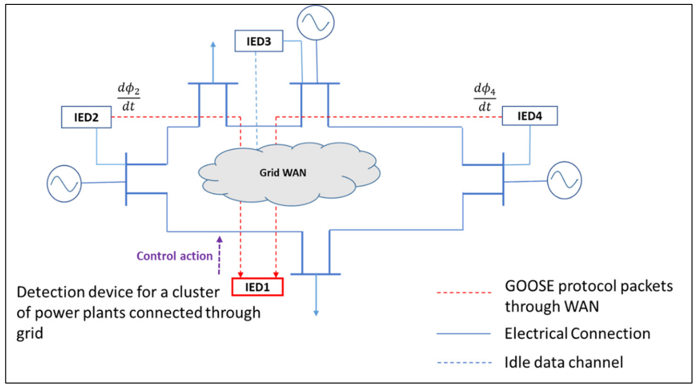
The GOOSE temporal based packets are published on the communication network of the electrical power grid by the Intelligent Electronic Device (IED), measuring the generator’s bus angle, such as a typical numerical protection relay. The detecting IED, which is another numerical protection IED with special settings to subscribe to the published GOOSE packets, will evaluate the stability of the rotor angle of the generator that publishes the GOOSE. Figure 1 shows the data communication network connecting the measuring IEDs to the central detecting IED. The GOOSE operation with a varying angle is detailed in [13]. Due to the very high speed of GOOSE transmission (typically less than 3 ms [20]), the detecting device can simultaneously receive many GOOSE streams from several disturbed generators and process them, thereby evaluating the stability of the entire grid.

According to the GOOSE protocol, the transmission packet occurs when its dataset value changes. In our scheme, the dataset is a set of Boolean variables where each variable corresponds to a prescribed angle boundary. The angle boundaries are prescribed every $${\phi }_{step}$$ degrees starting from 0. When the angle curve crosses one of the prescribed boundaries while increasing, the Boolean variable k corresponding to that boundary changes from zero to one. When the curve crosses the same boundary while decreasing, the same Boolean variable changes from one to zero. Therefore, upon each change in the Boolean variables corresponding to a quantized angle change, a GOOSE packet is transmitted immediately.

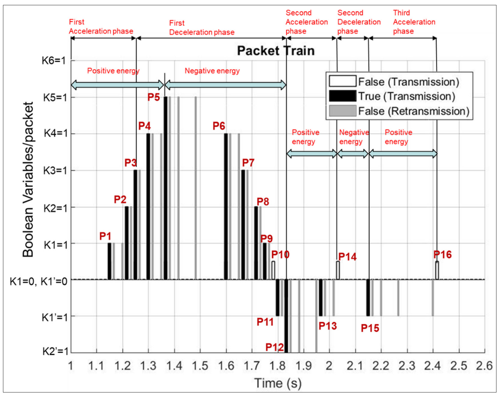
Figure 2 shows an example case of an oscillating AC power generator where $${\phi }_{step}$$ is taken as 30 degrees in this example. Figure 3 depicts the induced GOOSE packets from a varying angle. The Boolean sequence of each transmitted GOOSE packet (k′_n, …, k′₁, k₁, ..., k_n) is shown in black color. The following criteria determine the value of the Boolean variables:

where, β_n is the nth prescribed phase boundary corresponding to the Boolean variable k_n and β_n > 0. The zero-angle level is halfway between β₁ and −β₁.

The retransmission packets (shown in grey in Figure 3) are published with the same Boolean sequence as the last transmission packet when there is no data change for a defined time interval. So, if the angle curve continues without reaching the next lower or the higher boundaries, the first retransmission will occur after a time T, where T is taken to be the periodic time of the sinusoidal system frequency $${\omega }_{0}/2\pi$$. The selection of T to be the system’s sinusoidal wave periodic time coincides with the time window of the numerical relays that samples the wave periodically for a time T to evaluate the voltage phasor magnitude and phase angle. Thus, any change in the voltage phase will not be calculated before the time T elapses, and hence the GOOSE transmission packet will be triggered after the same time duration.

The acceleration or deceleration phase can be identified from the generated GOOSE pattern by observing the Boolean content of successive GOOSE transmission packets and the time interval between every two successive packets. For example, in Figure 3, during the first oscillation cycle, when the transmission packets (in black color) get closer with time, or in other words, the number of retransmissions (in grey color) decreases with time while the Boolean sequence of the packets is incrementing, this indicates an acceleration phase. This is depicted in Figure 3 for the packets from one to three (P1 to P3), where the Boolean sequence (k′₂, k′₁, k₁, k₂, k₃, k₄, k₅, k₆) increments from (0, 0, 1, 0, 0, 0, 0, 0) to (0, 0, 1, 1, 0, 0, 0, 0) then to (0, 0, 1, 1, 1, 0, 0, 0) in the packets P1, P2 and P3 respectively. When the number of retransmissions increases with time while the Boolean sequence is still incrementing, this will indicate a subsequent decelerating phase, and the speed of the generator’s rotor is still higher than the nominal speed $${\omega }_{0}$$ and consequently, the rotor’s kinetic energy exceeds its value at nominal speed. This is depicted in Figure 3 by the fourth and fifth packets, P4 and P5. When the Boolean sequence decrements from (0, 0, 1, 1, 1, 1, 1, 0) in packet P5 to (0, 0, 1, 1, 1, 1, 0, 0) in packet P6, the deceleration cycle continues, however, the rotor’s speed drops below the nominal and the kinetic energy drops below its initial value at nominal speed.

According to the GOOSE protocol, the duration between retransmissions is doubled consecutively. Thus, if the curve proceeds further without crossing the next lower or the higher boundaries, the second retransmission will occur at 2T, the third at 4T, and the fourth at 8T, and so on. The time between two successive GOOSE transmission packets can be estimated based on the summation of the time between all retransmissions lying between the two successive transmission packets.

Since the retransmission time follows a geometric series with base 2 and first term equal to T, then we can sum the retransmission times between any two successive packets by the following expression:

where, k is the retransmission order and m is the last retransmission No. between two successive packets.

Now, we know that the time between two successive packets (expressed as multiples of T) lies between kth and the kth + 1 total $$ReTx\mathrm{ }\,time$$, therefore:

where $${n}_{i}$$ is the ith integer multiple of T and $${n}_{i}\mathrm{T}$$ is the time duration between the ith packet and the packet preceding it.

Thus, for example, if there are two retransmissions observed between two transmission packets, the time between these two packets is 3T < $${n}_{i}\mathrm{T}$$ ≤ 7T, Therefore, $${n}_{i}$$ can take values from 4 to 7. Thus, Inequality (13) reveals that there is a range of possible values for $${n}_{i}$$. Table 1 displays the estimated time between two successive packets according to the number of retransmissions between both packets.

Since the speed varies continuously during acceleration and deceleration phases, then the exact value of $$∆\omega$$ presents the instantaneous deviation in angular speed during both phases.

The instantaneous $$∆\omega$$ value cannot be measured from the GOOSE stream, however the average speed can be calculated over a given angular range. The average speed variation over an interval between the packet number $$i$$ and the packet number $$\left(i-1\right)$$ preceding it is:

where, $$∆\varphi$$ is the angle change between the ith and the ith − 1 packets and $$T=\frac{2\pi }{{\omega }_{0}}$$

Therefore, from Equation (7), the estimated change in kinetic energy from the initial value at nominal speed, based on the average speed computed in Equation (14), is:

The sign of the energy in the above expression depends on the sign of $$∆\varphi$$. If $$∆\varphi$$ is positive, then the energy is acquired, if $$∆\varphi$$ is negative, the energy is dissipated.

During acceleration with positive energy: $${n}_{i}<{n}_{i-1},$$ while during deceleration with positive energy, the reverse is true. During acceleration with negative energy: $${n}_{i}>{n}_{i-1},$$ while during deceleration with negative energy, the reverse is true.

Since we are interested in evaluating the generator’s stability, we have to track the value of $${∆E}_{i}\mathrm{ }$$ in Equation (15) to find out whether it ceases at zero.

According to Equation (14), in Figure 3, the average speed variation from the nominal value in the interval between the fault inception time at 1 s and the first GOOSE packet during the first acceleration phase is:

where, $${n}_{1}$$ > $${n}_{2}$$.

Therefore, from Equation (16), the estimated kinetic energy acquired by the rotor in the time interval between the fault inception time and the first GOOSE packet is:

Since there is one retransmission packet observed between the second and the third packet compared to two transmission packets between the first and second packets, then $${n}_{3}<{n}_{2}$$. From Table 1, for two retransmissions, the time between the first and the second packets lies between 4T and 7T, therefore, $${n}_{3}<{n}_{2}<{n}_{1}$$. Thus, the generator undergoes its first acceleration cycle between the fault inception time and the third packet. It can also be seen in Figure 3 that there is one retransmission packet between the third and fourth packets, indicating that the rotor does not accelerate further between the third and fourth packets; thus, it can be considered the starting packet of the subsequent deceleration phase.

From the above argument, it can be concluded that the excess kinetic energy at the third packet, which constitutes the maximum energy acquired in the first acceleration phase, is:

It can also be noticed from Figure 3 that there are two retransmissions between the fourth and the fifth packets, therefore, $${n}_{5}<{n}_{4}$$, thus, according to Equation (14), the rotor definitely decelerates after the fourth packet, thus, the rotor starts to dissipate the acquired energy described by the above expression in Equation (18) during subsequent packets in deceleration phase.

Now, using Equation (15) and considering the negative angle change of $$∆\varphi$$ from the fifth to the sixth packet, the energy at the sixth packet yields a drop in the rotor’s kinetic energy below the initial value given by the following expression:

Equation (18) and Equation (19) reveal that the excess kinetic energy that has been acquired by the generator’s rotor during the acceleration phase is dissipated successively between the consecutive GOOSE packets during the deceleration phase until it fully ceases, then the rotor’s kinetic energy continues to decrease—due to its inertia—below its initial value at nominal speed, resulting in negative $$∆E$$. Subsequently, the rotor enters another acceleration phase starting from the interval between the eleventh and twelfth packets, and the cycle repeats.

From the above discussion, it can be concluded that the kinetic energy of the rotor, once turned to negative, identifies a stable oscillation cycle. This fact coincides with the equal area criterion of stability of power systems. However, in a real power system, the first peak in the oscillation is not necessarily the only peak; there may be other peaks with lower or higher amplitudes in later oscillation cycles. In the unstable case, the oscillation may exhibit higher subsequent peaks due to many factors, such as a lack of damping or inadequate action of Automatic Voltage Regulators (AVRs), Power System Stabilizers (PSSs), and governor loops. These factors may lead to growing amplitudes of oscillation with time. Thus, the equal area criterion can be applied for the first oscillation cycle only, not for the subsequent cycles in a multi-swing system. Therefore, we need another criterion for the stability assessment of power systems based on the temporal dynamics of energy flow.

From Equation (15), one can write:

where $${∆E}_{i}^{+}$$ is the positive energy, N is the number of packets with positive energy in the same acceleration-deceleration cycle. We will classify the power swing into three basic types, namely, Oscillatory (stable or unstable), Slow (non-oscillatory, stable or unstable), and Fast Monotonic Unstable swings.

The unstable oscillation implies that the rotor spans a wider angular range with positive energy in one of the oscillation cycles compared to that spanned by the rotor with positive energy in the cycle preceding it.

Since the quantized angular range spanned by the rotor during a positive energy cycle is $$N{\varphi }_{step}$$, then, the right-hand side of Equation (20) is proportional to this angular range. Therefore, the stability criterion for the oscillating angle can be formulated as:

where, $${∆E}_{i}^{+}$$ is the positive energy (excess energy above initial value) at the ith packet of the current oscillation cycle, $${n}_{i}$$ is the ith integer multiple of T for $${∆E}_{i}^{+}$$ duration, $${∆E}_{j}^{+}$$ is the positive energy at the jth packet of the subsequent oscillation cycle, $${n}_{j}$$ is the jth integer multiple of T for $${∆E}_{j}^{+}$$ duration. N is the last packet with positive energy in the current cycle and M is the last packet with positive energy in the subsequent cycle.

In case the rotor’s speed is always higher than the nominal speed, the kinetic energy never goes below the original value at nominal synchronous speed, thus $$∆E$$ is always positive. However, the rotor’s speed may drop to values near the nominal before it increases again, as in the case of slow oscillatory swings, therefore, from Equation (15), $$∆E$$ will approach zero in these intervals. In this case, the excess kinetic energy of the rotor oscillates above this low energy value, where it decays with time in case of a slow stable swing, or it increases with time in case of a slow unstable swing. The low energy level will be considered the level corresponding to 4 retransmissions or more between two successive GOOSE packets. The number of 4 retransmissions is selected as a limit because, from Table 1, $${n}_{i}$$ will range from 16 to 31, therefore $$∆E$$ will range from $$\frac{J{{\omega }_{0}}^{2}{\varphi }_{step}}{16}$$ and $$\frac{J{{\omega }_{0}}^{2}{\varphi }_{step}}{31}$$. For $${\varphi }_{step}=30\,\mathrm{ }degrees\mathrm{ }\,or\,\mathrm{ }\pi /6$$ radians, $$∆E$$ will lie between 1/16 and 1/32 approximately of the initial kinetic energy value, i.e., between 3% and 6% of the initial kinetic energy, which indicates that the rotor’s energy in this interval is very close to its initial kinetic energy before swing. In the same sense, for the time interval between two successive packets where more than 4 retransmissions exist, $$∆E$$ to initial kinetic energy ratio will be even lower, and the rotor’s energy will be closer to its initial value. This low $$∆E$$ level can be regarded as a quasi-stable state where all the acquired energy has been dissipated except a very low amount that can be dissipated during subsequent oscillation cycles for the stable swing case. Therefore, $${∆E}_{i}^{+}$$ and $${∆E}_{j}^{+}$$ will be estimated for all packets before and after this quasi-stable state, and the Inequality (21) will be checked to evaluate stability.

From Equation (20) and Inequality (21), the stability criterion can be set as:

Thus, for a stable swing:

Therefore, for the oscillations to be stable, the M count of GOOSE packets in one positive-energy cycle must be less than the N count of GOOSE packets in the preceding positive-energy cycle, where the energy between the two cycles either turns to negative or constitutes a quasi-stable level. Nevertheless, to account for the probability of errors in the digital quantization process, the practical stability criterion will be:

This implies that the instability criterion will be:

The stability assessment scheme relies on the detection of the angular range of positive energy in successive cycles based on the GOOSE transmission packets’ behavior as illustrated above; thus, the detecting device evaluates N and M in the successive cycles, which is a direct indication of the quantized kinetic energy values.

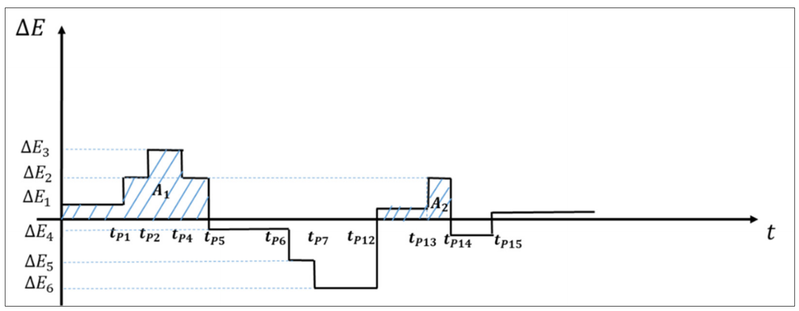
From Inequality (21), it can be seen that the stability criterion depends simply on the area under the positive $$∆E$$ part of the energy-time curve in both the current and the subsequent acceleration-deceleration cycles. At the same time, this area is proportional to the GOOSE packet count in each cycle. Figure 4 depicts an estimated curve of energy versus time for the oscillatory stable case of Figure 3 showing the areas under first and second positive energy portions of the curve.

If the swing is fast and monotonic, i.e., if the rotor always accelerates without an interim period of slowing down, then the acquired kinetic energy $$∆E$$ will be generally increasing and will never drop to a quasi-stable low energy level as in the above cases. However, in real power systems during unstable swings, the rotor speed may slow down in some intervals without approaching the nominal speed before stepping up again towards instability. In this case, the number of retransmissions may stay constant for several consecutive intervals, thus according to Equation (20), this yields a constant $$∆E$$ where the rotor speed is approximately constant. From the theory of synchronous machines, the electrical torque will be equal to zero at a rotor angle of 180 degrees, and this is the onset of out of step condition since any further increase in the angle will make the rotating field of the stator winding lose synchronism completely with the rotor’s winding field. However, during the constant energy levels, the rotating field of the stator winding has approximately the same speed as the rotor’s winding field, which is higher than the nominal speed of the machine. Therefore, the angle between the two fields will have minimal change during these intervals, although the apparent angle is still increasing relative to the initial angle value before disturbance. This difference results from computing the angle assuming that the two phasors are still rotating with the initial speed, while they are actually rotating with the new, higher speed. Thus, the two fields can be considered almost locked to each other during these constant energy intervals, and hence the measured angle would not be counted in the real 180-degree angular margin preceding the out of step condition. This constant energy value can be considered a quasi-stable state of the machine with nearly constant rotor angle, where the real angle increase will be computed with the subsequent energy increase after this quasi-stable level.

The above argument implies that the real out of step condition should be detected by the continuous speed increase and consequently the continuous energy increase, not just by the apparent angle increase.

Figure 5 depicts a typical monotonic unstable swing, and Figure 6 shows the induced GOOSE packets from the angle variations in this monotonic swing. Figure 6 shows interim periods of energy with nearly constant values. It can be seen that the packets from the second to the fifth are separated by one retransmission, then from Equation (15):

Therefore, there is a quasi-stable high energy state in this interval:

From Table 1, for one retransmission: $${n}_{3}=2\mathrm{ }\,or\,\mathrm{ }3$$ the quasi-stable energy value for $${\varphi }_{step}=30\,\mathrm{ }degrees$$ is either $$\frac{1}{4}J{{\omega }_{0}}^{2}$$ or $$\frac{1}{6}J{{\omega }_{0}}^{2}$$ approximately, i.e., the first quasi-stable energy value $${E}_{Q1}=$$ half the initial kinetic energy value or one third of it.

The packets from the fifth to the seventh are separated by two retransmissions, which signifies another quasi-stable energy level with a lower value than the first one, where,

From Table 1, $${n}_{6}$$ will be from 4 to 7, then,

i.e., $${E}_{Q2}$$ will lie between one seventh and one fourth of the initial kinetic energy.

From the seventh to the eighth packets, one retransmission is observed, which indicates an increase in energy again to $${E}_{Q1}$$ level. It can then be deduced from $$∆E$$ pattern that it falls to a lower value $${E}_{Q2}$$ but it is still well above the initial kinetic energy value as it reaches one seventh of it as a minimum, it does not fall near zero as in the case of slow swing illustrated above.

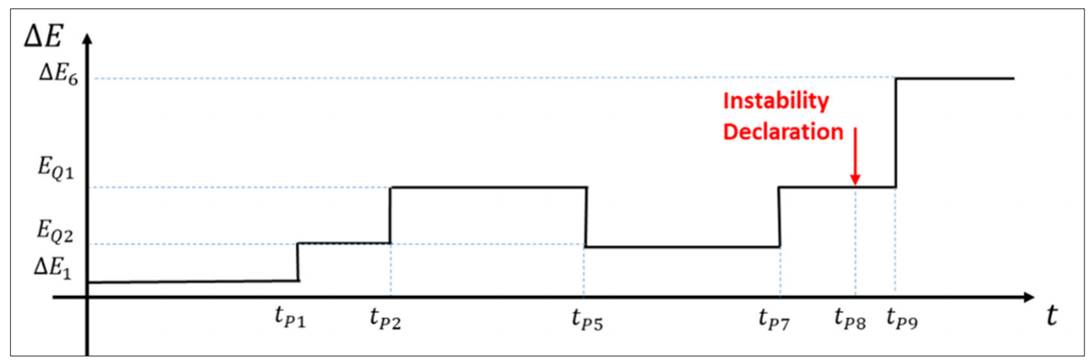
It can be recalled from Sections 3.3.1 and 3.3.2 that in the stable swing case, $$∆E$$ either turns to a negative value or approaches zero, although it may rise again in subsequent cycles. However, as demonstrated in Section 3.3.4, in the monotonic unstable case, $$∆E$$ never turns negative or approaches zero, but rather re-increases after a temporary drop. As mentioned in Section 3.3.2, if the number of retransmissions between successive GOOSE packets is less than 4, the energy drop will still retain a considerable amount of energy in the rotor, and hence, the excess kinetic energy cannot be considered zero. This temporary drop in energy before rising again to $${E}_{Q1}$$ implies the rotor failure to dissipate most of its energy during the relevant deceleration cycle, which infers that it will gain higher values during subsequent cycles, therefore, the instability has to be declared once the energy value steps up from $${E}_{Q2}$$ to $${E}_{Q1}$$. The conditions for a fast monotonic swing can be summarized as follows:

The energy intervals with estimated constant energy constitute the first quasi-stable higher energy level:

The energy intervals with estimated constant energy constitute the second quasi-stable lower energy level:

The instability criteria are:

where, $$∆E$$ has always positive values.

This section presents the response of the new scheme to disturbances applied to the simulated IEEE 10-machine 39-bus system as per [12] for both stable and unstable cases. New England 39 bus is a 60 Hz, 10-generator system with 46 lines and with slack generator G2 at bus 31.

According to [12], a stable disturbance is simulated by creating a three-phase-ground fault on line 2–3 near bus 2 at 1 s. Then the fault is cleared by tripping the line 2–3 at the time instant 1.33 s. The Most Disturbed Generator Pair (MDGP) is G1–G5, with G1 being severely affected by the disturbance.

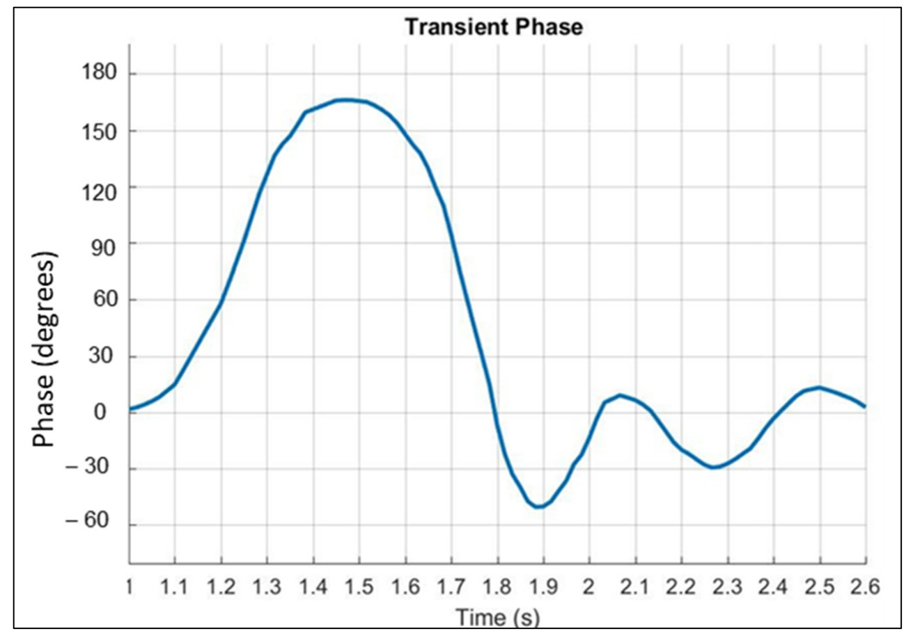
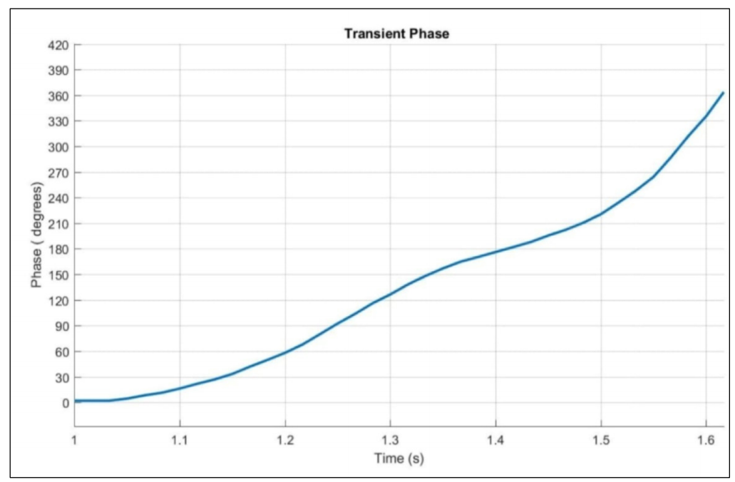
The stable case is depicted in Figure 2, where the relative angle of the MDGP is displayed versus time according to [12], which can be considered, in a reasonable approximation, as the worst case phase deviation for a disturbed generator relative to the grid in the proposed scheme. The GOOSE packets induced by the changing angle in the measuring device are generated using the Xelas IEC 61850 real-time simulator Version 6.0.3.5 (Xelas Energy Management, Marina Del Rey, CA, USA and The Hague, The Netherlands), and the detector device that receives the published GOOSE packets and assesses the stability is simulated using the same simulator on another PC connected via Local Area Network to the measuring device. The GOOSE packet train versus time, showing the Boolean sequence in each packet, is generated by MATLAB. Figure 3 displays the induced GOOSE at the varying angles shown in Figure 2.

To evaluate the kinetic energy in the second acceleration phase, the acceleration can be distinguished by the packets from P12 to P14, where the Boolean sequence increases from (−1, −1, 0, 0, 0, 0, 0, 0) to (−1, 0, 0, 0, 0, 0, 0, 0) then to (0, 0, 0, 0, 0, 0, 0, 0), therefore, $$∆E$$ is positive within these packets. The second deceleration phase is distinguished by the packets P14 and P15, where the Boolean sequences of the packets P14 and P15 are (0, 0, 0, 0, 0, 0, 0, 0) and (−1, 0, 0, 0, 0, 0, 0, 0) respectively. Therefore, the positive energy packets are from P12 to P14.

The detector device evaluates the integers N and M for each oscillating generator. N will be evaluated upon reception of the packet corresponding to the first Boolean sequence decrement, while M will be evaluated upon reception of the packet corresponding to the second Boolean sequence decrement. From Figure 3, the energy turns negative at the sixth packet, i.e., it remains positive for five consecutive packets, i.e., N = 5 in the first positive energy cycle, while in the second positive energy cycle, the energy remains positive for three consecutive packets only (P12 to P14), thus, M = 3 in the second acceleration phase. Therefore, from the Inequality (24), this oscillation is stable.

The stability will be declared after the fifteenth GOOSE packet P15 is received as it signals the turning point of energy to negative again and hence concludes the positive energy interval. As reported in our previous work in [13], the detection of a Boolean sequence increment or decrement in a GOOSE packet, relative to the sequence of the packet directly preceding it, takes approximately 4 ms. Thus, the stability of the oscillating generator will be declared after the detector device receives from the generator measuring device the GOOSE packet with the second decremented sequence by 4 ms, i.e., at time = 2.144 s approximately.

The energy versus time curve can be plotted as shown in Figure 4. It is worth noting here that since the scheme relies only on the GOOSE pulses count, $${∆E}_{i}$$ is not known exactly, since we know only the allowed quantum values for it, we only know exactly the total energy under the positive energy curve, which is $$\sum _{i=1}^{N}{∆E}_{i}^{+}·{n}_{i}$$. Therefore, $${∆E}_{i}$$ is estimated approximately for each packet, assuming one of the permissible values of $${n}_{i}$$ in Table 1 so as to match the exact total area under each positive energy cycle. This is only to show how the time-energy curve would look like. Figure 4 shows the quantized energy levels between the packets at the relevant packet emission time $${t}_{p1}$$ for P1, $${t}_{p2}$$ for P2 and so on. It can be seen that area A2 is less than area A1, which implies a stable swing. It can also be deduced that the positive energy packet counts before and after the negative energy cycle are proportional to A1 and A2, respectively.

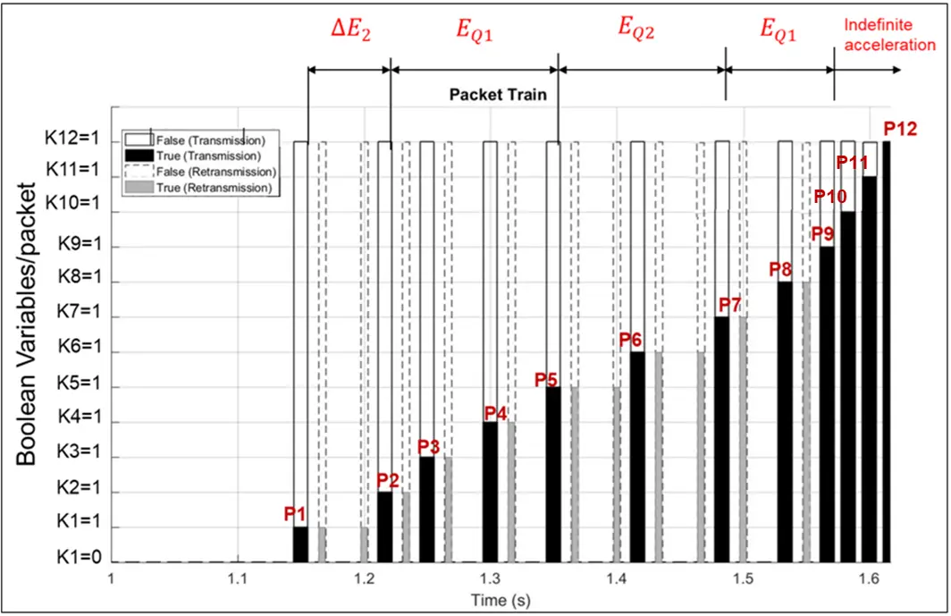
The unstable case is simulated according to [12] by increasing the fault clearing time to 1.331 s instead of 1.33. Figure 5 shows the relative angle of the MDGP according to [12], while Figure 6 displays the induced GOOSE by the varying angle of Figure 5.

Figure 6 shows equidistant GOOSE packets from P2 to P5 with one retransmission between every two successive packets, thus, from Section 3.3.4, $${∆E}_{3}={∆E}_{4}={∆E}_{5}$$ = $${E}_{Q1}$$ indicates the first quasi-stable level $${E}_{Q1}$$. While two retransmissions separate P6 from P5 and P7 from P6, this indicates the second quasi-stable level $${E}_{Q2}$$, where, $${E}_{Q2}<{E}_{Q1}$$. Then, from P7 to P8, back to one retransmission again, hence, $${∆E}_{8}>{E}_{Q2}$$. Therefore, the two Inequalities (32) and (33) hold, indicating a monotonic unstable swing.

The detector device will detect the decrease of retransmissions from 2 between the sixth and seventh to 1 between the seventh and eighth packets, and this condition signals the re-increase of the energy from $${E}_{Q2}$$ to $${E}_{Q1}$$. Hence, the detector will declare instability once the eighth packet is received. Thus, according to [13], the detector device will declare instability 4 ms later to the reception of the eighth packet, i.e., at the time = 1.537 s. Figure 7 depicts the estimated time-energy curve with the energy transitions at relevant packet emission times.

It can be noticed that the instability is declared at the packet corresponding to 240 degrees. As illustrated in Section 3.3.4, although this value exceeds the 180 degrees limit of out of step condition, the constant energy intervals with constant rotor speed imply that the rotating field and the rotor field are both rotating synchronously; therefore, there is no real angle change between them unlike the apparent angle. Considering the time-angle curve as a piecewise curve of constant energy intervals, the real 180 degrees out of step limit shall be counted as a sum of the angles at those intervals. Based on this new definition, in our example case, we have the successively increasing energy levels $$\mathrm{ }\,{∆E}_{1}$$, $$\mathrm{ }{∆E}_{2}$$, $${E}_{Q1}$$, where each level adds 30 degrees to the angle at the level preceding it. On the other hand, the energy is dropped from $${E}_{Q1}$$ to $${E}_{Q2}$$ which consequently subtracts 30 degrees from the angle at $${E}_{Q1}$$. Finally, the level $${E}_{Q2}$$ adds another 30 degrees to the angle at $${E}_{Q1}$$. Therefore, the real rotor angle progress is estimated as 90 degrees at the eighth and ninth packets.

It can be seen from Figure 6, that the generator accelerates continuously starting from the tenth packet. So, the real 180 degrees-rotor angle shift is expected to be at the twelfth packet, i.e., at the time = 1.62 s approximately. Nevertheless, due to the probability of errors between the real angle and the assumed constant angle in the quantization process, the out of step condition may happen slightly earlier. Thus, in all cases, the scheme remains capable of predicting impending instability early enough to enable the required control action.

Theoretically, if there is a very severe case where the angle increases monotonically without constant energy intervals, the instability will be declared directly by the detector device once the retransmission packets disappear completely.

To compare the effectiveness of the new scheme with other proposed WAMPAC techniques, the Auto-Regression technique proposed by [12] to predict unstable swings was reported to predict the instability for the same monotonic swing case at the time = 1.333 s. The Maximal Lyapunov Exponent (MLE)-based method was reported in [12] to declare instability at the time = 1.6 s.

The authors of [12] stated that the 180 degrees-apparent angle limit of instability is reached at the time 1.467 s, and they claimed accordingly that the MLE method declares the instability after the out of step condition actually occurs, while the Auto-Regression technique predicts the instability prior to its manifestation by 134 ms. Nevertheless, according to the quantized-energy estimation approach as pointed out in Section 4.1.2, the actual instability would occur at approximately 1.62 s. So, the fact is that the MLE detects the out of step condition before it happens, but with a very tight time margin for a remedial action to take place. On the other hand, the Auto-Regression predicts it too early, while the generator is actually in the first quasi-stable energy level. $${E}_{Q1}$$ as demonstrated in Section 4.1.2, and hence no accurate prediction is guaranteed. Finally, the new approach predicts instability about 87 ms before its manifestation, which is an adequate time for appropriate remedial action.

Another aspect of evaluating the new scheme is how its performance is affected by network errors in data transmission and network congestion or other network impairments. All of these factors may cause packet loss. However, in electrical utilities networks, the optical fiber is the main media used for communications, which gives more immunity against data transmission errors compared to wireless communications. Besides, the private fiber network suffers much less congestion than public networks like the Internet. In addition to this reduced possibility of packet loss, the GOOSE transmission mechanism does provide a means for tracking the packets since each packet has a state number once published with new data content, in addition, each retransmission packet has a sequence number once published with the same content [20]. Accordingly, if one GOOSE packet fails to reach its destination, the receiving IED will recognize this loss when the packet next to the lost one arrives by reading the last received packet state and sequence numbers. We will study the effect of losing one packet in the new scheme for the unstable swing case depicted in Figure 6, as it is the critical case to detect. Assume that the packet P2 is lost, then its retransmission, shown in grey next to it will arrive at the detecting IED. Once this retransmission packet is received, its sequence number will reveal that it is a retransmission; at the same time, its Boolean sequence shows an increment compared to the previous received packet, which is a second retransmission of P1. Hence, the detecting IED recognizes that packet P2 is lost and continues reading subsequent packets till it identifies the instability in its correct time after the P8 packet is received. The same argument is valid if any of the first received eight packets is lost except if P8 is lost. In this case, according to Section 4.1.2, the detecting IED will declare instability when the retransmission of P8 arrives 16.67 ms later. Therefore, the IED declares instability at the time 1.553 s instead of 1.537 s, thus, the time before actual instability reduces to 70.33 ms (compared to 87 ms if no packets are lost). Therefore, losing one packet can, in the worst case, reduce the allowable time for corrective action by one sinusoidal cycle or 16.67 ms. This reduction in the allowable time remains tolerable for fast remedial action.

A newly developed quantized rotor energy balance approach is introduced for power system stability assessment based on the WAMPAC GOOSE communication protocol, serving as a practical alternative to the Equal-Area Criterion. The approach utilizes the GOOSE packets emitted from the generator bus-angle measuring IED due to the bus angle change during the power swing. The change in rotor kinetic energy relative to the initial value at nominal rotor speed is estimated between every two consecutive GOOSE packets in a quantized form. The variable quantized rotor dynamic energy levels are then used to evaluate the stability of power systems during different types of swing, namely, oscillatory, slow, and fast monotonic swings. The detector IED counts the emitted GOOSE pulses from each disturbed generator IED through the WAMPAC network and hence can declare generator stability or predict instability before its actual manifestation by an adequate safe-response time to allow for remedial action. Being a PMU-independent technique, the new approach does not adopt synchronized measurements of rotor angles of multiple generators on the grid like PMU-based techniques; this eliminates the need for expensive PMUs and GPS synchronizing devices, as well as sufficient satellite coverage for all angle-measuring nodes in the grid. It has been demonstrated that for oscillatory swing, the energy curve versus time exhibits negative energy levels between quantized positive energy intervals; the areas under these positive energy parts of the curve have been proven proportional to the number of GOOSE packets emitted by the measuring IED during these intervals. Thus, comparing the GOOSE counts in these intervals by the detector IED determines the stability of the swing. It has also been demonstrated that the fast monotonic swing exhibits quasi-stable intermediate energy levels between two high-energy levels, and the scheme detects the transition to the second higher level as an indication of instability. The new approach is intrinsically asynchronous and does not require the expensive use of PMUs or synchronized phase measurements, thereby leveraging the direct application of protection relays and IEDs without complex synchronization requirements. Finally, the new approach introduces a new insight of the energy-time pulsed variations and energy measurement by the direct count of physical pulses. This differs radically from the most common techniques that rely on mathematical-based Equal Area Criterion and rotor angle estimation for power systems stability assessment.

The new approach can be deployed in grids with high renewable penetration. For example, deploying electrolyzers without optimal allocation may cause grid congestion where there are few transmission lines to evacuate the generated power [21]. Therefore, if a disturbance occurs on one of these lines or on a nearby generator, the power would automatically shift to other healthy lines, which are already operating near their thermal limits, which may cause overload cascaded failure of the remaining healthy lines. The new quantized energy approach can serve in predicting the impending instability resulting from the sudden disturbance on the congested grid, thus allowing for appropriate remedial action before cascaded failure.

Conceptualization, E.E.-M. and M.E.-S.; Methodology, E.E.-M.; Software, E.E.-M.; Validation, A.S.; Formal Analysis, E.E.-M.; Investigation, A.S.; Writing—Original Draft Preparation, E.E.-M.; Supervision, M.E.-S.

Not applicable.

Not Applicable.

Research data is available upon request.

This research received no external funding.

The authors declare that they have no known competing financial interests or personal relationships that could have appeared to influence the work reported in this paper.

References

- NERC. PRC-026-1—Relay Performance During Stable Power Swings; North American Electric Reliability Corporation: Washington, DC, USA, 2014. [Google Scholar]
- IEEE Power System Relaying Committee Working Group D6. Power Swing and Out-of-Step Considerations on Transmission Lines. 2006. Available online: https://www.ewh.ieee.org/r6/san_francisco/pes/pes_pdf/OutOfStep/PowerSwingOOS.pdf (accessed on 20 March 2026).
- Elmore WA. Protective Relaying Theory and Applications, 2nd ed.; Marcel Dekker: New York, NY, USA, 2004. [Google Scholar]
- Taylor CW, Haner JM, Hill LA, Mittelstadt WA, Cresap RL. A New Out-of-Step Relay with Rate of Change of Apparent Resistance Augmentation. IEEE Trans. Power Appar. Syst. 1983, PAS-102, 631–639. DOI:10.1109/TPAS.1983.317984 [Google Scholar]
- Tziouvaras DA, Hou D. Out-of-step protection fundamentals and advancements. In Proceedings of the 57th Annual Conference for Protective Relay Engineers, College Station, TX, USA, 1 April 2004; pp. 282–307. [Google Scholar]
- Rebizant W, Feser K. Fuzzy logic application to out-of-step protection of generators. In Proceedings of the 2001 Power Engineering Society Summer Meeting, Vancouver, BC, Canada, 15–19 July 2001; pp. 927–932. DOI:10.1109/PESS.2001.970179 [Google Scholar]
- Kundu P, Pradhan AK. Wide area measurement based protection support during power swing. Int. J. Electr. Power Energy Syst. 2014, 63, 546–554. DOI:10.1016/j.ijepes.2014.06.009 [Google Scholar]
- Abdelaziz AY, Irving MR, Mansour MM, El-Arabaty AM, Nosseir AI. Adaptive protection strategies for detecting power system out-of-step conditions using neural networks. IEE Proc. Gener. Transmiss. Distrib. 1998, 145, 387. DOI:10.1049/ip-gtd:19981994 [Google Scholar]
- Hashiesh F, Mostafa HE, Helal I, Mansour MM. A wide area synchrophasor based ANN transient stability predictor for the Egyptian Power System. In Proceedings of the IEEE PES Innovative Smart Grid Technologies Conference Europe (ISGT Europe), Gothenberg, Sweden, 11–13 October 2010; pp. 1–7. DOI:10.1109/ISGTEUROPE.2010.5638923 [Google Scholar]
- Hosseini SA, Taheri B, Abyaneh HA, Razavi F. Comprehensive power swing detection by current signal modeling and prediction using the GMDH method. Prot. Control Mod. Power Syst. 2021, 6, 15. DOI:10.1186/s41601-021-00193-z [Google Scholar]
- Farantatos E, Huang R, Cokkinides GJ, Meliopoulos AP. A Predictive Generator Out-of-Step Protection and Transient Stability Monitoring Scheme Enabled by a Distributed Dynamic State Estimator. IEEE Trans. Power Delivery 2016, 31, 1826–1835. DOI:10.1109/TPWRD.2015.2512268 [Google Scholar]
- Wei S, Yang M, Qi J, Wang J, Ma S, Han X. Model-Free MLE Estimation for Online Rotor Angle Stability Assessment with PMU Data. IEEE Trans. Power Syst. 2018, 33, 2463–2476. DOI:10.1109/TPWRS.2017.2761598 [Google Scholar]
- Chandra A, Pradhan AK. Model-free angle stability assessment using wide area measurements. Int. J. Electr. Power Energy Syst. 2020, 120, 105972. DOI:10.1016/j.ijepes.2020.105972 [Google Scholar]
- El-Metwally EA, Attia MA, El-Shimy M. A non-PMU-based WAN protection scheme for swing detection and stability enhancement in power systems. Electr. Eng. 2023, 105, 3191–3208. DOI:10.1007/s00202-023-01843-1 [Google Scholar]
- Padiyar KR. Power System Dynamics: Stability & Control; Wiley: Hoboken, NJ, USA, 1999. [Google Scholar]
- Centeno V, Phadke AG, Edris A, Benton J, Gaudi M, Michel G. An adaptive out-of-step relay [for power system protection]. IEEE Trans. Power Deliv. 1997, 12, 61–71. DOI:10.1109/61.568226 [Google Scholar]
- Paudyal S, Ramakrishna G, Sachdev MS. Application of Equal Area Criterion Conditions in the Time Domain for Out-of-Step Protection. IEEE Trans. Power Deliv. 2010, 25, 600–609. DOI:10.1109/TPWRD.2009.2032326 [Google Scholar]
- Kundur P. Power System Stability and Control; McGraw-Hill: New York, NY, USA, 1994. [Google Scholar]
- Krause PC, Wasynczuk O, Sudhoff SD. Analysis of Electric Machinery and Drive Systems; IEEE Press/Wiley: Hoboken, NJ, USA, 2025. [Google Scholar]
- IEC 61850-8-5; Communication Networks and Systems for Power Utility Automation—Part 5: Communication Requirements for Functions and Device Models. Technical Committee TC 57—Power Systems Management and Associated Information Exchange. International Electrotechnical Commission: Geneva, Switzerland, 2022. [Google Scholar]
- Giannelos S, Konstantelos I, Pudjianto D, Strbac G. The impact of electrolyser allocation on Great Britain’s electricity transmission system in 2050. Int. J. Hydrogen Energy 2026, 202, 153097. DOI:10.1016/j.ijhydene.2025.153097 [Google Scholar]