Distinguishing IGBT Open-Circuit Faults from DoS-Induced Anomalies in Smart Grids

Distinguishing IGBT Open-Circuit Faults from DoS-Induced Anomalies in Smart Grids

Received: 04 February 2026 Revised: 10 March 2026 Accepted: 23 March 2026 Published: 02 April 2026

© 2026 The authors. This is an open access article under the Creative Commons Attribution 4.0 International License (https://creativecommons.org/licenses/by/4.0/).
1. Introduction
The grid-tied power electronic inverters serve as a key interface between distributed energy resources and modern smart grids. Their reliability is therefore critical to secure and stabilize grid operation. Among inverter components, insulated gate bipolar transistors (IGBTs) are particularly susceptible to open-circuit faults, which can distort phase currents, accelerate component aging, and degrade grid stability [1]. Meanwhile, as a typical cyber–physical system (CPS), smart grids are also vulnerable to denial-of-service (DoS) attacks that disrupt the information layer and degrade effective control actions at the physical layer [2,3]. Consequently, a practical diagnosis scheme should not only localize IGBT open-circuit faults but also distinguish them from DoS-induced anomalies, which remains challenging for many circuit-dependent methods [4].
Existing inverter open-circuit fault diagnosis methods can be broadly categorized into voltage-based, current-based, and data-driven approaches. Voltage-based methods typically diagnose faults by detecting deviations between reference and measured voltages [5,6] or by monitoring switch-related voltages, such as the collector–emitter voltage [7]. However, many voltage-based schemes require additional voltage sensing circuitry [8,9], increasing cost and potentially reducing operational reliability. Sensorless voltage-observer methods have also been reported [10], but their performance is often sensitive to modeling accuracy and parameter uncertainties. Current-signal-based methods can reuse existing current measurements without extra hardware [11,12,13], yet they may require signal processing such as Fourier or wavelet transforms, leading to a higher computational burden. Observer-based current diagnosis methods (e.g., Luenberger, sliding-mode, and nonlinear observers) improve robustness to load variations and avoid additional sensors [14], but they still depend on modeling fidelity. Data-driven approaches (e.g., spectrum analysis, fuzzy logic, and neural networks) [15,16,17] can achieve good accuracy but often introduce higher complexity and implementation challenges.
The sliding mode observer has the advantage that the estimation error converges to zero in a finite time, and at the same time, it is not sensitive to the uncertainty of the system [18], but the observed value has a chattering problem, which decreases the estimation accuracy. Interval estimation can effectively improve the accuracy of state estimates, and the effective combination of interval estimation and sliding mode observer can not only improve the convergence speed of the sliding mode observer but also effectively reduce chattering and improve the robustness of the fault diagnosis system [19].
This paper addresses the problem of anomaly diagnosis in grid-tied inverters operating in cyber–physical smart grids, with the objective of distinguishing physical IGBT open-circuit faults from anomalies induced by denial-of-service (DoS) cyber-attacks. To this end, a second-order interval sliding-mode observer based on the super-twisting algorithm (STA) is developed to estimate inverter currents and generate structured residuals for reliable anomaly detection and discrimination. The main contributions of this paper are summarized as follows:
- (1)
-
A unified model-based anomaly diagnosis framework is established for grid-tied three-phase inverters in cyber-physical smart grids, where physical IGBT open-circuit faults and DoS-induced cyber anomalies are jointly modeled and distinguished within the same analytical framework.
- (2)
-
A super-twisting-based second-order interval sliding-mode observer (SOISMO) is developed for three-phase current estimation. Compared with conventional first-order sliding-mode observers, the proposed observer introduces a continuous second-order correction mechanism into the interval observer, thereby improving estimation smoothness, alleviating chattering, and preserving robustness against bounded disturbances and model uncertainties.
- (3)
-
An analytical residual-based fault localization criterion is derived for single-switch and same-leg double-switch open-circuit faults using residual sign patterns and 2:1 magnitude relationship. In contrast to existing residual-threshold-based cyber-attack detection methods, the proposed method exploits structural residual patterns to distinguish physical open-circuit faults from DoS-induced anomalies without requiring additional sensors, training data, or heuristic classifiers.
- (4)
-
Simulation studies demonstrate that the proposed method achieves reliable anomaly detection and discrimination within one fundamental cycle, while providing smoother current estimation and lower residual oscillation than the conventional interval sliding-mode observer.
Therefore, the objective of this paper is not only to diagnose inverter open-circuit faults, but also to distinguish them from DoS-induced cyber anomalies within a unified cyber-physical diagnosis framework.
2. DoS Attacks and Physical Faults in Inverters
This section establishes a unified modeling framework for inverter-based systems subject to both physical open-circuit faults and communication-induced anomalies. In practical cyber–physical energy systems, inverter operation may be simultaneously affected by hardware-level physical faults, such as IGBT open-circuit failures, and network-layer uncertainties arising from DoS attacks or packet losses in communication channels. Although these two types of anomalies originate from different physical layers, they both manifest as abnormal behaviors in the measured current signals.
To enable reliable anomaly detection and fault localization under such hybrid conditions, a closed-loop inverter model incorporating both physical fault mechanisms and stochastic communication effects is developed.
2.1. Smart Grid Model under DoS Attacks
From the viewpoint of inverter fault diagnosis, the essential impact of short-term DoS attacks lies not in the network protocol itself, but in the effective degradation or intermittency of control actions acting on the physical system. Over short time scales, such effects can be equivalently represented as bounded disturbances or attenuation in the inverter current dynamics. This perspective enables cyber-induced anomalies to be analyzed and distinguished within a unified model-based diagnosis framework.
Neglecting the IGBT dead-time effect, the grid-tied inverter is approximated by a linear discrete-time plant:
where $$x\left(k\right)\in {\mathbb{R}}^{n}$$ is the state, $$u\left(k\right)\in {\mathbb{R}}^{m}$$ is the control input, $$z\left(k\right)\in {\mathbb{R}}^{q}$$ is the controlled output, and $$\omega \left(k\right)\in {\mathbb{R}}^{p}$$ denotes an exogenous disturbance. The matrices $$A$$, $${B}_{2}$$, $${B}_{1}$$, $$C$$, and $$D$$ are known and of compatible dimensions.
To capture communication-induced uncertainties, the sensor-to-controller (S–C) and controller-to-actuator (C–A) channels are modeled as unreliable links subject to random packet losses. A standard hold-last-sample (zero-order-hold) mechanism is adopted: when a packet is lost, the most recent sample is held. The packet-loss process is modeled as
where $${x}_{c}\left(k\right)\in {\mathbb{R}}^{n}$$ is the state received by the controller, and $$\theta \in \mathrm{\Theta }=\left\{{\theta }_{1},\dots ,{\theta }_{s}\right\}$$ denotes the information-layer mode. Similarly, the controller-to-actuator channel is modeled by
where $${u}_{c}\left(k\right)\in {\mathbb{R}}^{m}$$ is the control command generated by the controller.
The Bernoulli random variables $${\delta }_{1}^{\theta }$$ and $${\delta }_{2}^{\theta }$$ indicate packet loss: $${\delta }_{i}^{\theta }=1$$ implies a dropout (holding the previous value), whereas $${\delta }_{i}^{\theta }=0$$ implies successful transmission. They satisfy
where $${b}_{1}^{\theta },{b}_{2}^{\theta }\in \left[0,\mathrm{ }1\right]$$ are the packet-loss probabilities for the sensor-to-controller and controller-to-actuator links, respectively.
To account for the impact of communication uncertainties on the control action, a mode-dependent state-feedback controller is considered as
where $${K}^{\theta }\in {\mathbb{R}}^{m×n}$$ is the controller gain.
Substituting Equation (2), Equation (3), Equation (4) and Equation (5) into Equation (1) yields the closed-loop system with random packet loss:
with
and
Moreover,
Note: In this work, logic variables and Bernoulli random variables play different roles. The logic variable δ ∈ {0,1} is used to describe current-direction-dependent physical fault behaviors, whereas the Bernoulli packet-loss variables $${\delta }_{1}^{\theta }$$ and $${\delta }_{2}^{\theta }$$ in Equation (2) and Equation (3) model stochastic communication losses.
Remark 1. Interpretation of $${h}_{i}^{\theta }$$ and $${t}_{i}^{\theta }$$.
The coefficients $${h}_{i}^{\theta }$$ ($$i=1, 2, 3$$) are deterministic weights determined by the packet-loss probabilities $${b}_{1}^{\theta }$$ and $${b}_{2}^{\theta }$$, reflecting the average contributions of the current state and delayed states associated with the hold-last-sample mechanism. In contrast, $${t}_{i}^{\theta }$$ capture the stochastic deviations between the actual dropout realizations $$\left({\delta }_{1}^{\theta },{\delta }_{2}^{\theta }\right)$$ and their mean values $$\left({b}_{1}^{\theta },{b}_{2}^{\theta }\right)$$. Hence, the closed-loop dynamics Equaitons (6) and (7) can be viewed as a nominal delay system perturbed by bounded random terms induced by DoS-related communication intermittency, which motivates a robust observer-based residual generation for anomaly diagnosis in the subsequent sections.
It is worth emphasizing that physical faults and communication anomalies are characterized by different modeling mechanisms in this work. Logic variables are introduced to describe deterministic fault-related behaviors, such as current-direction-dependent conduction paths under IGBT open-circuit faults.
In contrast, stochastic Bernoulli random variables are employed to model communication-induced packet losses, which represent the random effects of DoS attacks or network congestion. By embedding both mechanisms into the same closed-loop dynamics, the resulting model captures the combined impact of hardware faults and cyber-induced anomalies on inverter operation.
2.2. The Inverter Model under Single IGBT Fault
In Figure 1, $${u}_{an}$$, $${u}_{bn}$$, and $${u}_{cn}$$ denote the three-phase voltages in a microgrid.
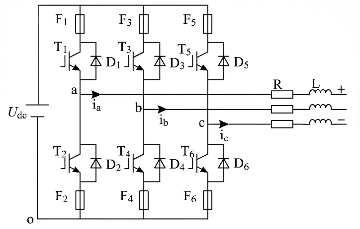
Figure 1. Equivalent circuit of the inverter, where $${T}_{1}$$–$${T}_{6}$$ are the IGBT switches, $${D}_{1}$$–$${D}_{6}$$ are the diodes, and $${i}_{a}$$, $${i}_{b}$$, $${i}_{c}\,$$denote the three-phase currents.
Taking phase-$$c$$ as an example, the model in Figure 1 is simplified using ideal electronic switches. Thus, the IGBT switches $${T}_{5}$$ and $${T}_{6}$$ are represented by the switching functions $${S}_{5}$$ and $${S}_{6}$$, respectively. Similarly, $${T}_{1}$$–$${T}_{4}$$ are represented by $${S}_{1}$$–$${S}_{4}$$. When $${S}_{5}=1$$, switch $${T}_{5}$$ is commanded ON (i.e., healthy operation in the switching command as listed in Table 1). If $${S}_{6}=0$$ due to an open-circuit fault of $${T}_{6}$$, the lower switch cannot conduct even when commanded. When an open-circuit fault occurs only in $${T}_{5}$$, the resulting pole-voltage behavior is summarized in Table 1, where $${u}_{co}^{\mathrm{\prime}}$$ denotes the pole voltage under the $${T}_{5}$$ fault.
Table 1. Truth table of $${u}_{co}^{\mathrm{\prime}}$$ under an open-circuit fault of $${T}_{5}$$.
|
S5 |
S6 |
δc |
u'co |
|---|---|---|---|
|
0 |
0 |
1 |
0 |
|
0 |
1 |
1 |
0 |
|
1 |
0 |
1 |
0 |
|
0 |
0 |
0 |
Udc |
|
0 |
1 |
0 |
0 |
|
1 |
0 |
0 |
Udc |
Accordingly, $${u}_{co}^{\mathrm{\prime}}$$ can be expressed as
When only $${T}_{5}$$ has an open-circuit fault, the phase voltages are
From Equation (14), when only $${T}_{5}$$ has an open-circuit fault, the current dynamics can be written as
from Equation (15), the current residual dynamics under the $${T}_{5}$$ open-circuit fault are
assuming that the initial value of the state residual of the three-phase current is 0, solving Equation (16) can obtain
According to Equation (17), when the fault occurs only in $${T}_{5}$$, the residuals satisfy $$\mathrm{\Delta }{i^\prime}_{a}\le 0$$, $$\mathrm{\Delta }{i^\prime}_{b}\le 0$$, and $$\mathrm{\Delta }{i^\prime}_{c}\ge 0$$, with $$|\mathrm{\Delta }{i^\prime}_{c}|=2|\mathrm{\Delta }{i^\prime}_{a}|=2|\mathrm{\Delta }{i^\prime}_{b}|$$ over the corresponding conduction interval. The 2:1 magnitude relationship originates from the structural coefficient matrix of the three-phase inverter voltage transformation in Equation (14). Specifically, the faulty phase current residual is associated with the coefficient 2, while the two healthy phases are associated with the coefficient −1. As a result, the analytical solution of the residual dynamics in Equation (17) naturally leads to the deterministic magnitude relationship $$\mid \mathrm{\Delta }{i^\prime}_{c}\mid =2\mid \mathrm{\Delta }{i^\prime}_{a}\mid =2\mid \mathrm{\Delta }{i^\prime}_{b}\mid$$. This ratio is therefore not heuristic but directly derived from the inverter circuit structure.
For physical fault modeling, the logical variable $${\delta }_{c}\in \left\{0,1\right\}$$ is introduced to describe the current-direction-dependent freewheeling diode conduction in phase-$$c$$. Specifically, $${\delta }_{c}=1$$ corresponds to positive phase current with the lower-leg diode conducting, while $${\delta }_{c}=0$$ corresponds to a negative phase current with the upper-leg diode conducting. This modeling approach is commonly adopted in open-circuit fault analysis of two-level three-phase inverters.
2.3. The Inverter Model under Two IGBTs Faults in the Same Phase
When the two IGBT switches $${T}_{5}$$ and $${T}_{6}$$ on phase-$$c$$ have open-circuit faults at the same time, the specific analysis results are shown in Table 2, where $${u}_{co}^{\prime\prime}$$ represents the voltage at $${T}_{5}$$ and $${T}_{6}$$, where open-circuit faults occur simultaneously.
Table 2. Truth table of pole voltage $${u}_{co}^{\prime\prime}$$ under simultaneous open-circuit faults of $${T}_{5}$$ and $${T}_{6}$$.
|
S5 |
S6 |
δc |
u''co |
|---|---|---|---|
|
0 |
0 |
1 |
0 |
|
0 |
1 |
1 |
0 |
|
1 |
0 |
1 |
0 |
|
0 |
0 |
0 |
Udc |
|
0 |
1 |
0 |
Udc |
|
1 |
0 |
0 |
Udc |
Based on Table 2, when both $${T}_{5}$$ and $${T}_{6}$$ suffer open-circuit faults, the pole voltage of phase-$$c$$ is independent of the switching commands and can be expressed as
When open-circuit faults occur in the IGBT switches $${T}_{5}$$ and $${T}_{6}$$ at the same time, the phase voltage of each phase is
The current dynamics under simultaneous open-circuit faults of $${T}_{5}$$ and $${T}_{6}$$ can be written as
Accordingly, the current residual satisfies
Assuming zero initial residuals, the solution of the residual dynamics is
According to Equation (22), when open-circuit faults occur to $${T}_{5}$$ and $${T}_{6}$$ at the same time, the current residuals of phase $$a$$, $$b$$, and $$c$$ can be positive or negative, but the value of the current residuals of phase $$c$$ is as twice large as the value of phase $$a$$ and $$b$$, that is, the faulty phase can be located through the relationship between the three-phase current residuals. It follows that, under the same-leg double-switch open-circuit faults, the residuals of the two healthy phases have identical magnitude and opposite sign to half of the faulty-phase residual, while the faulty-phase residual has twice the magnitude. Therefore, the faulty phase can be reliably identified based on the residual sign and ratio.
2.4. The Inverter Model under Two IGBTs Faults in Different Phase
Taking the open-circuit faults of the $${T}_{4}$$ and $${T}_{5}$$ IGBT switches simultaneously occurring in the $$b$$ and $$c$$ phases as an example, using the modeling method of the simultaneous open-circuit faults of the two switches in the same phase, the specific details of $${u}_{bo}^{\prime\prime\prime}$$ and $${u}_{co}^{\prime\prime\prime}$$ can be obtained as
When open-circuit faults occur to the IGBT switches $${T}_{4}$$ and $${T}_{5}$$ at the same time, the phase voltage of each phase is
According to Equation (24), the current when open-circuit faults occur to the IGBT switches $${T}_{4}$$ and $${T}_{5}$$ at the same time is
According to Equation (25), the current residual when open-circuit faults occur to the IGBT switches $${T}_{4}$$ and $${T}_{5}$$ at the same time is
Assuming that the initial value of the state residual of the three-phase current is 0, solving Equation (26) can get
It follows from Equation (27) that in a cycle, the current residuals of the faulty phase and the healthy phases do not maintain a constant 2:1 magnitude relationship over the entire cycle, so the numerical relationship cannot be used to locate the faulty phase and the faulty tube in one cycle.
However, within specific switching intervals, the residuals still exhibit a 2:1 magnitude relationship, enabling interval-based fault localization. For example, when the IGBT switch $${T}_{5}$$ is normally disconnected or $${T}_{6}$$ is in the conduction interval, that is when $${s}_{5}$$ = 0 or $${s}_{6}$$ = 1, the three-phase current residual expression is:
It can be obtained from Equaiton (28) that in this interval, the current residuals of phases $$a$$ and $$c$$ are both non-negative, and the current residuals of phase-$$b$$ are non-positive and are twice the value of phase-$$a$$ and phase-$$c$$. Based on the residual sign pattern and the magnitude relationship, the faulty switch can be identified for the corresponding interval.
When the IGBT switch $${T}_{4}$$ is in the interval of normal disconnection, that is, when $${s}_{4}$$ = 0, the expression of the three-phase current residual is:
It can be obtained from Equation (29) that in this interval, the current residuals of phase $$a$$ and $$b$$ are both non-positive, and the current residuals of phase-$$c$$ are non-negative and are twice the value of phase-$$a$$ and phase-$$b$$. According to the positive and negative of the current residuals and the relationship between the residuals, it can be judged which IGBT switch in which phase the open-circuit fault occurs.
In summary, single-tube fault and in-phase double-tube fault diagnosis methods are the basis of out-of-phase double-tube fault diagnosis methods. The out-of-phase double tube fault is a special case of a single tube fault. Also taking the faults of the $${T}_{4}$$ and $${T}_{5}$$ tubes as an example, when $${T}_{5}$$ is normally disconnected or $${T}_{6}$$ is in the period of conduction, the current residual relationship at this time is $$\mathrm{\Delta }{i}_{c}=-2\mathrm{\Delta }{i}_{a}=-2\mathrm{\Delta }{i}_{b}\ge 0$$, which is the current residual relationship when the open-circuit fault occurs to $${T}_{5}$$ tube. Therefore, the single-tube fault location method can be applied over different intervals to identify the faulty phase and tube when an out-of-phase dual-tube fault occurs. Therefore, this article focuses on the inverter single-tube open-circuit fault and the in-phase double-tube open fault.
In this way, the above-mentioned method can also deal with the open-circuit fault of the phase-$$a$$ and phase-$$b$$ IGBT switches, and the current residuals of the phase-$$a$$ and phase-$$b$$ under different fault conditions can be obtained. The current residual information table of each phase when open-circuit faults occur to a single switching tube and two IGBT switches in the same phase at the same time is shown in Table 3.
Table 3. The current residual information table for each phase.
|
Phase |
IGBT |
Residual Relationships |
|---|---|---|
|
3-Pha |
— |
Δiₐ = Δib = Δic = 0 |
|
T1 |
Δiₐ = −2Δib = −2Δic ≥ 0 |
|
|
a |
T2 |
Δiₐ = −2Δib = −2Δic ≤ 0 |
|
T1 & T2 |
Δiₐ = −2Δib = −2Δic |
|
|
T3 |
Δib = −2Δiₐ = −2Δic ≥ 0 |
|
|
b |
T4 |
Δib = −2Δiₐ = −2Δic ≤ 0 |
|
T3 & T4 |
Δib = −2Δiₐ = −2Δic |
|
|
T5 |
Δic = −2Δiₐ = −2Δib ≥ 0 |
|
|
c |
T6 |
Δic = −2Δiₐ = −2Δib ≤ 0 |
|
T5 & T6 |
Δic = −2Δiₐ = −2Δib |
It should be noted that the residual sign and 2:1 magnitude ratio pattern in Table 3 are derived analytically from the inverter dynamics and do not rely on data-driven training or heuristic thresholds. This property forms the theoretical basis for fault localization and for distinguishing open-circuit faults from DoS-induced anomalies.
The unified closed-loop model derived in this section serves as the basis for subsequent anomaly diagnosis. In particular, while both physical faults and DoS-induced communication anomalies disturb the inverter currents, their effects on the system dynamics exhibit fundamentally different structural characteristics. This observation motivates the observer-based residual generation and fault localization strategy developed in the next section, where physical open-circuit faults are identified through deterministic residual sign and magnitude patterns, whereas DoS-induced anomalies lead to attenuated residual responses without such structured features.
3. Second Order Sliding Mode Observer
It should be emphasized that this section does not aim to develop a new inverter control strategy. Instead, the super-twisting mechanism is introduced as an estimation and correction tool embedded into the observer design, with the primary objective of improving current estimation accuracy, robustness, and residual quality for anomaly diagnosis. The underlying inverter control architecture, including synchronization and current regulation, is assumed to follow standard grid-connected inverter practice and is not the focus of this paper.
To meet the diagnostic objective, the observer is designed based on reduced-order current dynamics of the inverter rather than a full, high-order switching-level model. This choice is consistent with the widely adopted principle of model order reduction in electrical engineering, where the dominant state dynamics relevant to estimation and diagnosis are retained while unnecessary switching-level details are omitted. As a result, the observer remains analytically tractable and computationally suitable for real-time implementation, while preserving the fault-sensitive current dynamics required for residual generation and anomaly discrimination.
This section summarizes the super-twisting mechanism and the interval estimation components used in this work, with emphasis on their integration to construct a robust current observer for anomaly diagnosis.
3.1. Super-Twisting Algorithm
A Super-Twisting Algorithm (STA) can be given as follows:
The output $$x$$ converges in finite time and remains in a neighborhood of $$x=0$$ in the presence of bounded uncertainties and disturbances. In Equation (30), $$f$$ is the disturbance of arbitrary Lipschitz bounded uncertainty, $${k}_{1}$$ and $${k}_{2}$$ are constants that can guarantee finite-time convergence to the second sliding mode $$x\left(t\right)={x}^{\mathrm{\prime}}\left(t\right)=0$$. For $$t>T$$, the first derivative of $$x$$ is not required by the controller implementation. For this one-dimensional system, the STA can be viewed as an output-feedback controller.
In Figure 2, the reference values $${i}_{dref}$$ and $${i}_{qref}$$ of the current inner loop are calculated by using the instantaneous power theory. The current loop is improved based on the sliding mode control algorithm, and an integral term is introduced based on the sliding mode surface to eliminate the error. In the switching control stage, the super-twisting control rate is introduced, and the switching functions $${S}_{d}$$ and $${S}_{q}$$ are obtained. Finally, the space vector pulse width modulation (SVPWM) is used to generate a pulse signal to drive the IGBTs. SVPWM is employed here as a standard modulation technique to generate gate signals for the inverter and does not affect the observer design. The phase-locked loop (PLL) is assumed to provide grid synchronization and is not involved in the proposed diagnosis strategy. It is noted that the super-twisting algorithm (STA) represents the core second-order sliding-mode mechanism, while the term super-twisting sliding-mode control (STSMC) refers to its implementation within a conventional inverter current-loop structure. In this work, the STA principle is not used to synthesize a new control law; instead, it is exploited as an estimation and correction mechanism embedded in the observer to enhance robustness and reduce chattering in current estimation.
Remark 2. On Reduced-Order Modeling.
The observer is established on the dominant current dynamics of the grid-tied inverter rather than on a full electromagnetic switching model. This can be interpreted as a diagnosis-oriented reduced-order representation, where the states most relevant to current estimation, residual generation, and anomaly propagation are preserved. Such a reduced-order formulation decreases computational burden and facilitates observer synthesis without sacrificing the essential dynamic signatures associated with open-circuit faults and DoS-induced anomalies.
3.2. Super-Twisting Sliding Mode Control Strategy
The inverter control loop considered in this work adopts a super-twisting sliding-mode structure, which serves as the nominal inner-loop configuration for observer design and analysis.
The robustness of the system is improved, and the dynamic characteristics of the converter are enhanced. The overall block diagram of the energy storage converter system designed in this paper is shown in Figure 2.
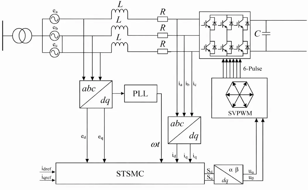
In Figure 2, the current inner loop uses the reference values $${i}_{dref}$$, $${i}_{qref}$$, and the current outer loop improvement algorithm, based on the sliding mode control algorithm, introduces the integral term based on the sliding surface to eliminate the error. In the switching-control stage, the super-twisting law is applied to obtain the switching functions $${S}_{d}$$ and $${S}_{q}$$, and SVPWM is then used to generate gate pulses for the IGBTs.
The current inner loop is mainly to achieve a unity power factor grid connection and make the phase of the incoming current consistent with the voltage phase, so that the system can quickly reach a steady state. According to the sliding mode control theory and the requirements of current loop control, the current tracking error $$e$$ is defined as the difference between the reference current and the actual current, and then the sliding mode surface of the current loop can be designed as
The controller parameters are tuned in MATLAB/Simulink to achieve satisfactory current tracking performance. Since the error derivative will increase the signal-to-noise ratio in the actual system, an integral term is introduced on the sliding mode surface to eliminate steady-state tracking errors. Accordingly, the sliding-mode surfaces with integral terms are given by
According to the principle of sliding mode control, calculation shows that $$S$$ is a differentiable function whose derivative at $$t$$ is given by
Through the mathematical model of the inverter, using Clark transfer and Park transfer, which obtain Equation (33) in $$dq$$ coordinates
By substituting the sliding-mode-based control law into the inverter mathematical model, the following expressions are obtained:
In order to enable the energy storage inverter to be connected to the grid with close to unity power factor, the reactive current is always equal to 0. In actual working conditions, the switching frequency cannot reach infinity. Therefore, this paper introduces a saturation function whose expression is
where $$S$$ represents the switching function, and $$\mathrm{\Delta }$$ represents the error bound. The selection of $$\mathrm{\Delta }$$ is closely related to the control effect of the system. Generally, as $$\mathrm{\Delta }$$ decreases, the control of the system will increase, but at the same time, there will be an increase in the chattering of the system; on the contrary, the control effect of the system will be relatively poor, and the chattering effect will be weakened.
Therefore, after the experimental simulation, literature [20] takes a positive real number interval, so that the continuous control remains on the switching surface $$S=0$$. To alleviate chattering effects induced by dead zones and measurement noise, the super-twisting mechanism is employed to improve the convergence behavior while preserving robustness properties, which can not only make the state of the system reach the sliding mode surface in the effective time but also effectively improve the dynamics of the approaching motion. The control rate of the introduced super-twisting algorithm is:
By incorporating the super-twisting correction term, the effective switching functions used in the current loop can be expressed as:
To provide a design-oriented stability argument, define the Lyapunov candidate as follows:
Under the super-twisting structure in Equation (37) and bounded uncertainties, the closed-loop sliding variables can be rendered finite-time convergent to a neighborhood of the origin whose size is governed by the boundary-layer parameter $$\mathrm{\Delta }$$ and the gain selection $${\alpha }_{1},{\alpha }_{2}$$. In practice, $${\alpha }_{1}$$ mainly affects the reaching speed, while $${\alpha }_{2}$$ influences the attenuation of residual oscillations; excessively large gains may amplify measurement noise and compromise robustness. Therefore, the controller parameters are selected through simulation-based tuning to balance convergence speed, chattering suppression, and noise sensitivity.
3.3. Interval Sliding Mode Observer
To enhance robustness against bounded disturbances and modeling uncertainties, an interval sliding mode observer (ISMO) is adopted by combining interval estimation with sliding mode observation. Consider the linear system.
where $$x\left(t\right)\in {\mathbb{R}}^{n}$$ is the state vector, $$u\left(t\right)\in {\mathbb{R}}^{m}$$ is the control input, $$y\left(t\right)\in {\mathbb{R}}^{p}$$ is the measured output, and $$v\left(t\right)\in {\mathbb{R}}^{q}$$ denotes an unknown but bounded disturbance satisfying $${v}_{\mathrm{m}\mathrm{i}\mathrm{n}}\le v\left(t\right)\le {v}_{\mathrm{m}\mathrm{a}\mathrm{x}}$$. The matrices $$A$$, $$B$$, $$C$$, and $$D$$ are constant and of appropriate dimensions.
Assumptions
-
-
The pair $$\left(A,C\right)$$ is observable.
-
-
There exists a matrix $$E$$ such that $$F=A-EC$$ is Hurwitz and Metzler.
-
-
The disturbance $$v\left(t\right)$$ is bounded with known bounds $${v}_{\mathrm{m}\mathrm{i}\mathrm{n}}$$ and $${v}_{\mathrm{m}\mathrm{a}\mathrm{x}}$$.
Under these Assumptions, the upper- and lower-bound sliding mode observers can be designed as
where $${K}_{s}$$ is the sliding mode gain selected such that
The interval state estimate is obtained as a convex combination of the two observers as follows:
where the weighting factor $$\alpha \left(t\right)\in \left[0,\mathrm{ }1\right]$$ is defined by
To avoid numerical issues when $$C(\hat{x}^--\hat{x}^+)$$ becomes small, $$\alpha \left(t\right)$$ is implemented with a safeguard $$ϵ>0$$ as $$\alpha(t)=\frac{y-C\hat{x}^+}{\max\{C(\hat{x}^--\hat{x}^+),\epsilon\}}$$ and then saturated to $$\left[0,\mathrm{ }1\right]$$.
For the inverter system, the hybrid logic current model can be written as
where $$i\left(t\right)\in {\mathbb{R}}^{3}$$ denotes the three-phase current vector. Applying the above observer design yields the upper-bound and lower-bound current estimates, denoted by $$\hat{\iota}^+(t)\mathrm{~and~}\hat{\iota}^-(t)$$, respectively. The real-time current estimate is then constructed as
where $$\alpha \left(t\right)$$ is the interval weight factor
A residual-based anomaly decision rule can be defined based on the current residual as follows:
An anomaly is declared when the residual magnitude exceeds a predefined threshold.
where $$\rho >0$$ is selected according to the maximum residual bound under normal operating conditions.
Beyond simple anomaly detection, fault localization is achieved by exploiting the analytical sign and magnitude relationships among the three-phase residual components. Specifically, for open-circuit faults, the faulty phase is identified through the characteristic residual relationship.
where $${r}_{f}$$ denotes the residual of the faulty phase and $${r}_{h}$$ denotes the residual of each healthy phase. Together with the corresponding residual sign pattern, this relationship provides a deterministic criterion for locating the faulty switch or faulty phase.
By contrast, DoS-induced anomalies do not generate fixed sign structures or 2:1 magnitude ratio pattern. Instead, they mainly appear as attenuation-type residual responses caused by intermittent packet loss and temporary degradation of control effectiveness. Therefore, the proposed method goes beyond conventional residual-threshold-based cyber-attack detection approaches: it not only detects abnormal conditions but also distinguishes physical open-circuit faults from DoS-induced anomalies, enabling physical fault localization within a unified observer-based framework.
Remark 3. Difference from Conventional Sliding-Mode Observers.
The proposed observer differs from a conventional first-order sliding-mode observer in that the discontinuous first-order switching injection is replaced by a super-twisting-based second-order correction term. As a result, the observer does not require direct differentiation of the sliding variable and exhibits smoother estimation behavior with reduced high-frequency oscillation. In addition, unlike a conventional SMO that only provides a point estimate, the proposed method embeds the super-twisting mechanism into an interval-observer structure, thereby preserving upper- and lower-bound state estimation capability under bounded disturbances and modeling uncertainties. Therefore, compared with the conventional SMO and the standard ISMO, the proposed SOISMO combines finite-time convergence characteristics, interval robustness, and improved estimation smoothness, which is particularly beneficial for generating reliable residuals in anomaly diagnosis.
4. Fault Diagnosis and Simulation Analysis
A simulation model is established in MATLAB/Simulink to evaluate the proposed diagnosis method for grid-tied three-phase inverters under both physical and cyber-induced anomalies. Two anomaly types are considered: (І) IGBT open-circuit physical faults, and (ІІ) DoS-induced communication anomalies. The anomaly is introduced at time. $${t}_{0}$$ and cleared at time$$\,{t}_{1}.$$
To illustrate the diagnostic principle, a representative phase current channel is used as an example. Let $${i}_{a}^{nom}\left(t\right)$$ denote the nominal phase-a current under normal operation. Then, the two representative anomaly models are constructed as follows:
(І) Open-circuit fault (phase-$$a$$ current interruption):
(ІІ) DoS-induced anomaly (equivalent current attenuation caused by intermittent control actions):
where $$\beta \in \left(0,1\right)$$ denotes the attenuation level.
It should be emphasized that Equation (50) and Equation (51) are simplified representative models used for simulation illustration. The analytical diagnosis framework developed in Sections 2 and 3 is not limited to these specific expressions. In general, physical open-circuit faults introduce deterministic structural changes in the inverter current dynamics, whereas DoS-induced anomalies primarily manifest as stochastic attenuation or disturbance effects due to packet loss in communication channels.
It is assumed that an attacker can launch DoS-induced anomalies that intermittently block communication channels, resulting in random packet loss. Short-term network attacks at fixed intervals can be approximated as equivalent, with their impact on the inverter represented as bounded low-frequency disturbances in the current dynamics. Therefore, $$\beta$$ is used to parameterize the severity of the DoS-induced attenuation in the equivalent disturbance representation. It is assumed that a DoS attack intermittently blocks communication channels, leading to packet loss and temporary interruptions in the exchange of measurement or control information. From the inverter-side perspective, such packet dropouts cause intermittent control actions and zero-order-hold behavior. Over short attack intervals, their cumulative effect can be approximated as a bounded low-frequency disturbance or effective attenuation in the current dynamics. Therefore, the attenuation-based representation in Equation (51) is adopted as a practical equivalent model of DoS-induced communication degradation.
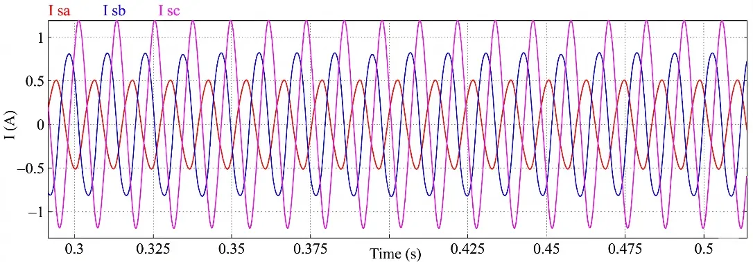
First, the inverter load is adjusted to induce variation in the three-phase currents, and the resulting current response is shown in Figure 3.
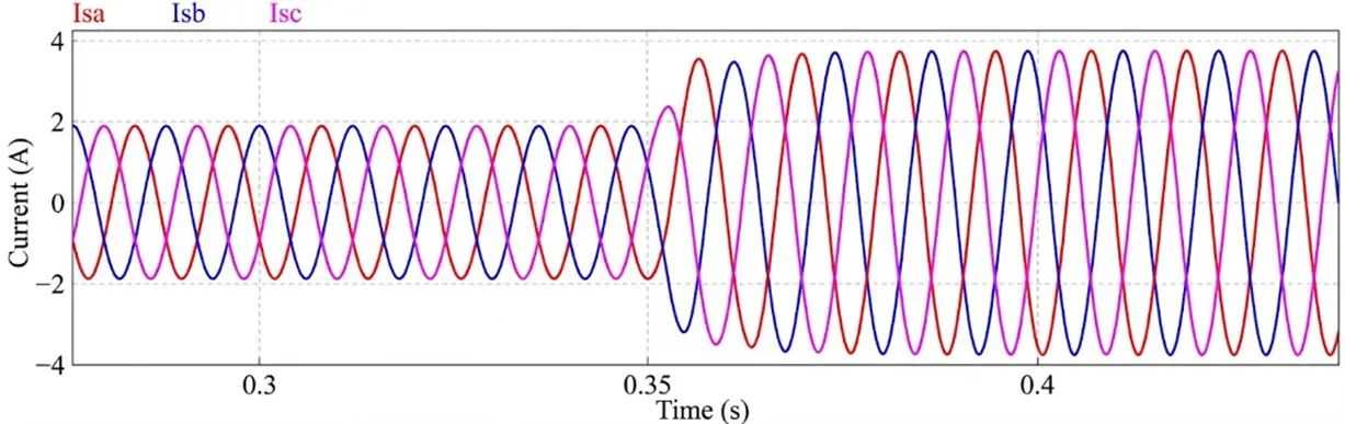
Considering practical operating constraints and protection limits, the attenuation level is set to $$\beta =0.25$$ in the simulation. Based on the measured three-phase currents shown in Figure 3, the estimation performance of the conventional interval sliding-mode observer and the proposed STA-based SOISMO is compared in Figure 4. The measured phase-a current is used as the reference signal.
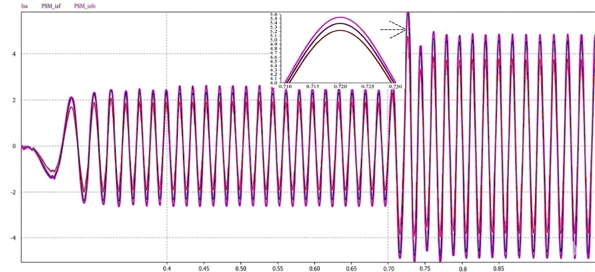
Figure 4. Comparison of phase-a current estimation results under the same operating condition: measured current (reference), conventional interval sliding-mode observer (ISMO), and the proposed STA-based second-order interval sliding-mode observer (SOISMO). A zoomed view of the steady-state interval is included to highlight the reduced oscillation and chattering of the proposed observer.
In Figure 4, the conventional ISMO can track the overall current trend, but its estimate exhibits more pronounced oscillatory behavior near the current peaks and zero crossings. By contrast, the proposed SO-ISMO provides a closer match to the measured current with smoother transient evolution and smaller estimation fluctuation. This improvement is attributed to the super-twisting-based second-order correction mechanism, which weakens the discontinuous switching effect typically observed in first-order sliding-mode injection. To explicitly demonstrate the chattering-suppression capability claimed in the observer design, Figure 4 should include either a zoomed steady-state comparison between the ISMO and the proposed SOISMO. The corresponding results show that the proposed observer yields lower high-frequency oscillation and reduced residual ripple under the same operating conditions. Therefore, compared with the conventional ISMO, the proposed SOISMO is more suitable for residual generation and subsequent anomaly discrimination. Taking phase-$$a$$ as an example, an open-circuit fault is emulated by forcing the phase-$$a$$ current to zero during $$\left[{t}_{0},{t}_{1}\right]$$, corresponding to a same-leg double-switch open-circuit condition in that phase.
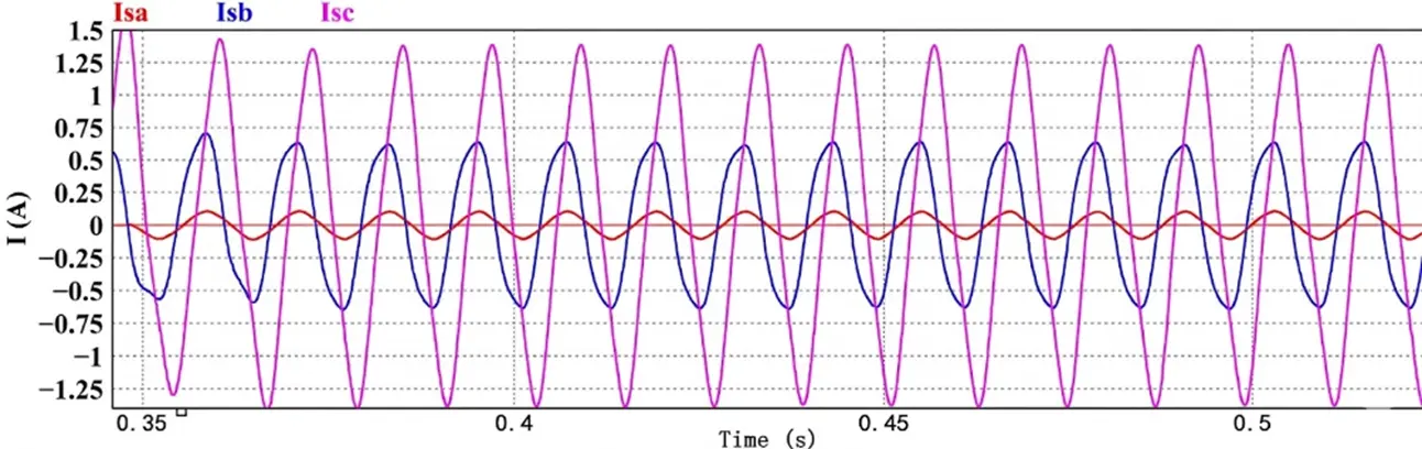
Figure 5 shows the inverter current response when an open-circuit fault occurs in phase-a. Under this condition, the phase-a current is forced to zero over the fault interval, while the remaining two phases currents remain nonzero but become distorted because of the coupling inherent in the three-phase inverter system. This behavior is consistent with the analytical fault model derived in Section 2.
Similarly, a DoS-induced anomaly is emulated by attenuating the phase-$$a$$ current by a factor of $$\left(1-\beta \right)$$ over $$\left[{t}_{0},{t}_{1}\right]$$, representing the short-term effect of intermittent control actions caused by communication packet dropouts under DoS attacks, which is consistent with the modeling assumption in Section 2. Figure 6 shows the inverter current response under the simulated DoS-induced anomaly. In this case, the phase-a current is not completely interrupted; instead, it is attenuated during the attack interval due to the equivalent degradation of control effectiveness caused by intermittent packet loss. Since the inverter remains grid-connected and the three phases are dynamically coupled, the other phase currents are also affected, but their responses differ from those under an open-circuit fault.
It is noted that, in Section 2, DoS-induced anomalies are modeled as packet dropouts in the communication channels, which lead to intermittent availability of measurement and control signals. From the inverter-side perspective, such packet dropouts result in intermittent control actions, where the control input is temporarily held by the zero-order-hold mechanism. Over short and periodic intervals, the cumulative effect of these intermittent control actions can be equivalently represented as bounded low-frequency disturbances or effective attenuation in the current dynamics. Therefore, the attenuation-based simulation model serves as a practical and physically meaningful approximation of DoS-induced communication degradation in networked inverter systems. When phase-$$a$$ is subjected to the DoS-induced communication degradation, the current of phase-$$a$$ will drop sharply and be much lower than the normal level. Since the inverter needs to be connected to the grid and the three-phase currents affect each other, the other two-phase currents will also be affected differently. This degradation can compromise stable grid operation.
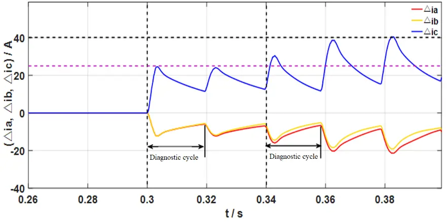
The proposed STA-based SOISMO is then applied to estimate the currents and generate residuals for anomaly diagnosis. The residual waveform is shown in Figure 7, a horizontal threshold (purple dashed line) is preset to distinguish normal operation from anomalous conditions. The vertical dashed lines mark the initiation of the diagnostic cycles once the residual exceeds this limit. When the residual exceeds the predefined threshold, the inverter is declared to be in an anomalous state. More importantly, the residual structure enables discrimination between physical faults and DoS-induced anomalies. For open-circuit faults, the residuals exhibit deterministic sign patterns and the characteristic 2:1 magnitude relationship among the faulty and healthy phases, in agreement with the analytical results derived in Section 2. By contrast, under DoS-induced anomalies, the residuals mainly reflect attenuation behavior and do not exhibit the same deterministic sign-ratio structure. This difference provides the basis for distinguishing physical switch faults from communication-induced anomalies. Overall, the simulation results verify that the proposed method not only detects abnormal operating conditions but also accurately differentiates open-circuit faults from DoS-induced anomalies within a unified observer-based diagnosis framework. In addition, compared with the conventional ISMO, the proposed SOISMO provides smoother current estimation and lower residual oscillations, thereby improving the reliability of residual-based decision-making.
5. Conclusions
This paper presented a super-twisting-based second-order interval sliding-mode observer for anomaly diagnosis in grid-tied three-phase inverters operating in cyber–physical smart grids. By integrating interval estimation with a super-twisting sliding-mode structure, the proposed observer achieves accurate current estimation with reduced chattering and enhanced robustness against bounded disturbances and modeling uncertainties.
From a modeling and analysis perspective, analytical residual relationships were explicitly derived for single-switch and same-leg double-switch IGBT open-circuit faults based on the inverter hybrid logic dynamics. These relationships reveal deterministic residual sign patterns and fixed 2:1 magnitude ratios among the three-phase currents, which enable reliable fault localization without requiring additional sensors, signal processing, or data-driven training. In contrast, DoS-induced anomalies were shown to primarily manifest as current attenuation effects without such deterministic residual structures, thereby allowing physical faults to be distinguished from cyber-induced anomalies within a unified observer-based framework.
Compared with existing current-based or voltage-based diagnosis approaches, the proposed method provides a model-driven and analytically grounded diagnosis mechanism that is well suited for cyber–physical environments, where both component-level faults and communication-induced anomalies may coexist. The ability to discriminate between these two anomaly types is particularly important for preventing false fault alarms and inappropriate protection actions in smart grid applications.
Simulation results demonstrated that the proposed approach achieves fast and reliable anomaly diagnosis under the considered operating conditions and attack scenarios. These results confirm the effectiveness of the proposed observer and residual-based decision rules in distinguishing IGBT open-circuit faults from DoS-induced anomalies.
Future work will focus on extending the proposed diagnosis framework to multi-converter and large-scale interconnected systems, as well as investigating coordinated cyber–physical attack scenarios and their impacts on distributed inverter-based power networks.
Author Contributions
Conceptualization, J.L. and Y.Z.; Methodology, J.L.; Software, J.L.; Validation, J.L. and Y.Z.; Formal Analysis, J.L.; Investigation, J.L.; Resources, Y.Z.; Data Curation, J.L.; Writing—Original Draft Preparation, J.L.; Writing—Review & Editing, J.L. and Y.Z.; Visualization, J.L.; Supervision, Y.Z.; Project Administration, Y.Z.; Funding Acquisition, Y.Z.
Ethics Statement
Not applicable.
Informed Consent Statement
Not applicable.
Data Availability Statement
The data that support the findings of this study are available from the corresponding author upon reasonable request.
Funding
This work is partially supported by the Natural Sciences and Engineering Research Council of Canada.
Declaration of Competing Interest
The authors declare that they have no known competing financial interests or personal relationships that could have appeared to influence the work reported in this paper.
References
- Panteli M, Mancarella P. The grid: Stronger, bigger, smarter? Presenting a conceptual framework of power system resilience. IEEE Power Energy Mag. 2015, 13, 58–66. DOI:10.1109/MPE.2015.2397334 [Google Scholar]
- Ding L, Han Q-L, Sindi E and Wang L. Distributed cooperative optimal control of DC microgrids with communication delays. IEEE Trans. Ind. Inform. 2018, 14, 3924–3935. DOI:10.1109/TII.2018.2799239 [Google Scholar]
- Bisello A, Vettorato D, Ludlow D, Baranzelli C. Smart and Sustainable Planning for Cities and Regions: Results of SSPCR 2019; Springer Nature: Cham, Switzerland, 2021. [Google Scholar]
- Gharaibeh A, Salahuddin MA, Hussini SJ, et al. Smart cities: A survey on data management, security, and enabling technologies. IEEE Commun. Surv. Tutor. 2017, 19, 2456–2501. DOI:10.1109/COMST.2017.2736886 [Google Scholar]
- Choi C, Seo E, Lee W. Detection method for open-switch fault in automotive PMSM drives using inverter output voltage estimation. In Proceedings of the IEEE Vehicle Power and Propulsion Conference (VPPC), Seoul, Republic of Korea, 9–12 October 2012; pp. 128–132. DOI:10.1109/VPPC.2012.6422626 [Google Scholar]
- An QT, Sun L, Sun LZ. Hardware-circuit-based diagnosis method for open-switch faults in inverters. Electron. Lett. 2013, 49, 1089–1091. DOI:10.1049/el.2013.0641 [Google Scholar]
- Shu C, Chen Y-T, Yu T-J, Wu X. A novel diagnostic technique for open-circuited faults of inverters based on output line-to-line voltage model. IEEE Trans. Ind. Electron. 2016, 63, 4412–4421.DOI:10.1109/TIE.2016.2535960 [Google Scholar]
- Beg OA, Nguyen LV, Johnson TT, Davoudi A. Signal temporal logic-based attack detection in DC microgrids. IEEE Trans. Smart Grid 2018, 10, 3585–3595. DOI:10.1109/TSG.2018.2832544 [Google Scholar]
- Kumar D, Zare F. A comprehensive review of maritime microgrids: System architectures, energy efficiency, power quality, and regulations. IEEE Access 2019, 7, 67249–67277. DOI:10.1109/ACCESS.2019.2917082 [Google Scholar]
- Freire NMA, Estima JO, Cardoso AJM. A voltage-based approach without extra hardware for open-circuit fault diagnosis in closed-loop PWM AC regenerative drives. IEEE Trans. Ind. Electron. 2014, 61, 4960–4970. DOI:10.1109/TIE.2013.2279383 [Google Scholar]
- Peuget R, Courtine S, Rognon J-P. Fault detection and isolation on a PWM inverter by knowledge-based model. IEEE Trans. Ind. Appl. 1998, 34, 1318–1326. DOI:10.1109/28.739017 [Google Scholar]
- Espinoza-Trejo DR, Campos-Delgado DU, Bárcenas E, Martínez-López FJ. Robust fault diagnosis scheme for open-circuit faults in voltage source inverters feeding induction motors using nonlinear PI observers. IET Power Electron. 2012, 5, 1204–1216. DOI:10.1049/iet-pel.2011.0309 [Google Scholar]
- Espinoza-Trejo DR, Campos-Delgado DU, Bossio G, Bárcenas E, Hernández-Díez JE, Lugo-Cordero LF. Fault diagnosis scheme for open-circuit faults in field-oriented control induction motor drives. IET Power Electron. 2013, 6, 869–877. DOI:10.1049/iet-pel.2012.0256 [Google Scholar]
- Jlassi I, Estima JO, El Khil SK, Bellaaj NM, Cardoso AJM. A robust observer-based method for IGBTs and current sensors fault diagnosis in voltage-source inverters of PMSM drives. IEEE Trans. Ind. Appl. 2017, 53, 2894–2905. DOI:10.1109/TIA.2016.2616398 [Google Scholar]
- Velasquez RMA, Mejia Lara JV. Expert system for power transformer diagnosis. In Proceedings of the IEEE International Conference on Electronics, Electrical Engineering and Computing (INTERCON), Cusco, Peru, 15–18 August 2017; pp. 1–4. [Google Scholar]
- Zidani F, Diallo D, Benbouzid MEH, Naït-Saïd R. A fuzzy-based approach for the diagnosis of fault modes in a voltage-fed PWM inverter induction motor drive. IEEE Trans. Ind. Electron. 2008, 55, 586–593. DOI:10.1109/TIE.2007.911951 [Google Scholar]
- Khan AA, Beg OA, Alamaniotis M, Ahmed S. Intelligent anomaly identification in cyber-physical inverter-based systems. Electr. Power Syst. Res. 2021, 193, 107024. DOI:10.1016/j.epsr.2021.107024 [Google Scholar]
- Yu X, Kaynak O. Sliding mode control made smarter: A computational intelligence perspective. IEEE Syst. Man Cybern. Mag. 2017, 3, 31–34. DOI:10.1109/MSMC.2017.2663559 [Google Scholar]
- Feng Y, Zhou M, Han Q-L, Han F, Cao Z, Ding S. Integral-type sliding-mode control for a class of mechatronic systems with gain adaptation. IEEE Trans. Ind. Inform. 2019, 16, 5357–5368. DOI:10.1109/TII.2019.2954550 [Google Scholar]
- Choi U-M, Lee J-S, Blaabjerg F, Lee K-B. Open-circuit fault diagnosis and fault-tolerant control for a grid-connected NPC inverter. IEEE Trans. Power Electron. 2016, 31, 7234–7247. DOI: 10.1109/TPEL.2015.2510224 [Google Scholar]