Comparing Drone and Satellite DEMs for Hydrodynamic Flood Modeling in a Rural Brazilian Catchment

Comparing Drone and Satellite DEMs for Hydrodynamic Flood Modeling in a Rural Brazilian Catchment
Amanda Ribeiro Lutterback Dias
*
 Antonio Krishnamurti Beleño de Oliveira
José Tavares Araruna Junior
Antonio Krishnamurti Beleño de Oliveira
José Tavares Araruna Junior
Received: 29 December 2025 Revised: 20 January 2026 Accepted: 09 March 2026 Published: 24 March 2026

© 2026 The authors. This is an open access article under the Creative Commons Attribution 4.0 International License (https://creativecommons.org/licenses/by/4.0/).
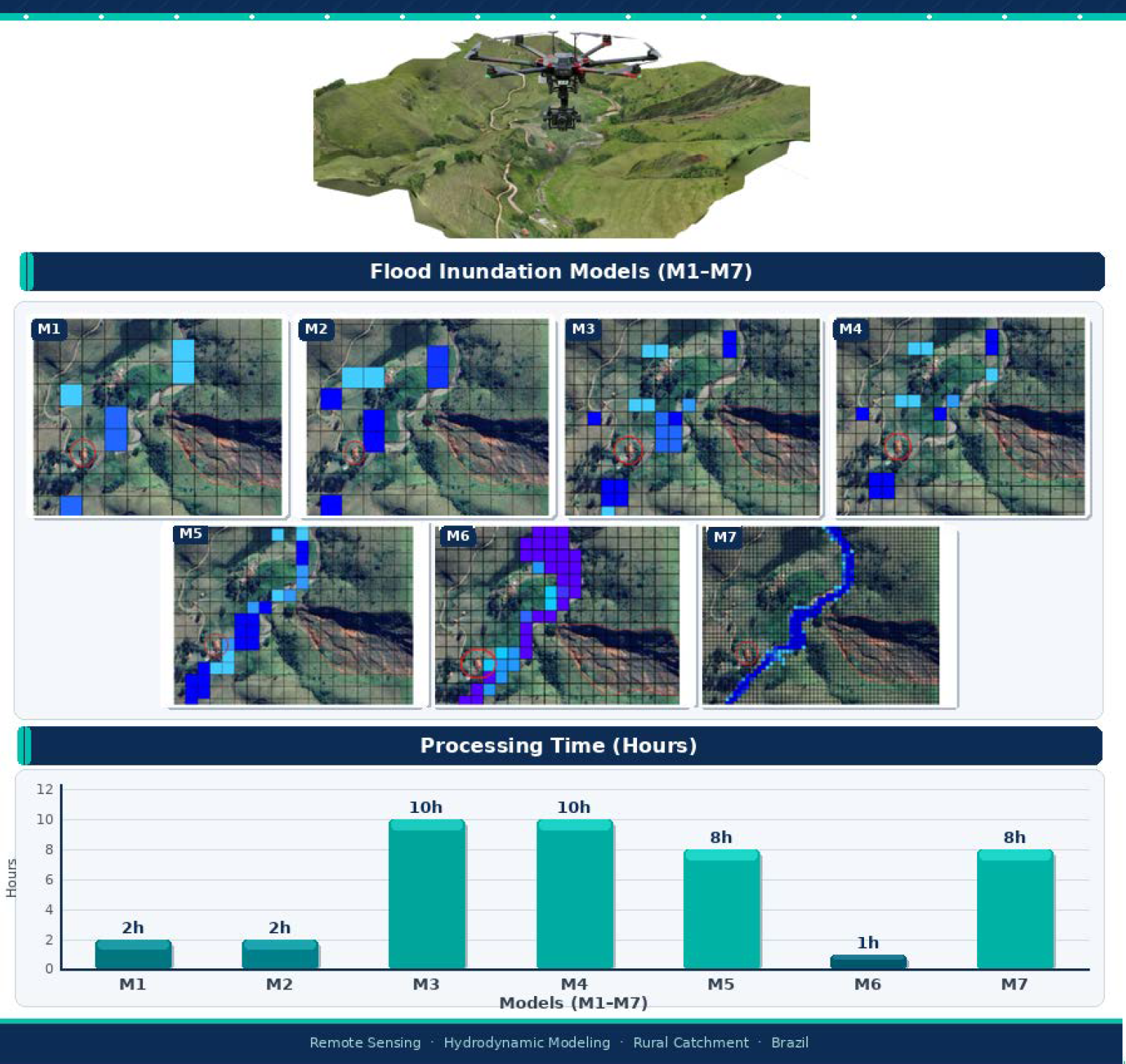
Graphical Abstract
1. Introduction
River floods are among the most frequent and impactful natural disasters globally, leading to substantial human, economic, and environmental losses. These events are caused by river overflows, usually associated with heavy rainfall, and primarily affect riverside areas [1]. It is estimated that these events were responsible for approximately seven million deaths worldwide throughout the 20th century [2]. It is predicted that exposure to flood risks could triple by 2050, driven by population growth and the concentration of assets in vulnerable areas [3]. In Brazil, especially in regions with rugged terrain and dispersed human settlement, these events are frequently aggravated by accelerated erosion processes, such as gully erosion. The phenomenon of gully erosion results from the combined action of multiple factors that promote the detachment and transport of materials on the earth’s surface [4]. Gullies are erosive features characterized by steep walls that evolve upstream through processes of undermining of the base and mass movements of the soil [5].
To analyze this type of problem, numerical modeling has become a fundamental tool in various areas of science and engineering, allowing the simulation and prediction of complex natural systems [6]. The development of numerical models involves steps such as problem definition, mathematical formulation, discretization, computational implementation, and validation, with continuous refinement being essential to ensure the accuracy and reliability of the results. Hydrological and hydrodynamic models are based on conservation principles and physical equations, using numerical techniques to integrate surface and subsurface runoff processes and reproduce hydrological responses in drainage basins [7]. By employing mathematical formulations to represent the hydrological cycle, modeling enables the analysis of the spatiotemporal dynamics of processes, the validation of theoretical hypotheses, and the projection of future scenarios [7]. To achieve this, several models have been developed over the last few decades, each with different approaches, levels of complexity, and specific objectives. Table 1 summarizes the main modeling programs, outlining their advantages, disadvantages, and typical applications. This summary aims to facilitate a comparative understanding between the models, highlighting their main characteristics and fields of use, in order to offer a clearer and more integrated view of their potential and limitations in the context of hydrological and environmental studies.
Table 1. Main hydrological and hydrodynamic models, with their respective advantages, disadvantages, and applications.
|
Model |
Advantages |
Disadvantages |
Main Uses |
|---|---|---|---|
|
HEC-HMS (Hydrologic Modeling System) |
|
|
|
|
SWMM (Storm Water Management Model) |
|
|
|
|
MODFLOW (Modular Finite-Difference Groundwater Flow Model) |
|
|
|
|
SWAT (Soil and Water Assessment Tool) |
|
|
|
|
MODEL (Cell Model) |
|
|
|
Source: Author (2025).
Table 2, presented below, brings together six studies that employed the methods discussed earlier, highlighting their main application and location. These examples show that research involving modeling is widely conducted in different parts of the world, with the aim of representing and understanding the behavior of physical systems, predicting scenarios, and supporting decision-making. It is worth noting that case studies using MODCEL are still scarce, especially internationally. This is because it is a relatively new model. In this context, this work also sought to demonstrate the effectiveness of this program.
Table 2. Studies using classical models and case studies.
|
Study |
Model(s) Used |
Main Application |
Local |
|---|---|---|---|
|
Netto et al. (2024) [8] |
SWAT, HEC-HMS |
Performance comparison for flood forecasting and basin management. |
Various international contexts |
|
Snikitha et al. (2024) [9] |
SWAT, HEC-HMS, SWMM |
Review of approaches for urban flood modeling and model selection. |
Urban environments |
|
Keller et al. (2022) [10] |
SWAT, HEC-HMS, MODFLOW |
Critical evaluation of models for water resource management and extreme events. |
Various contexts |
|
Aqnouy et al. (2023) [11] |
SWAT, HEC-HMS |
Flow simulation and flood risk assessment in a Mediterranean basin. |
Northern Morocco |
|
Qiu et al. (2021) [12] |
SWAT |
Monitoring of agricultural and rural floods. |
Pearl River Basin, China (rural) |
|
Bragg et al. (2025) [13] |
SWMM |
Comparison of SWMM and HEC-RAS in the hydrological response of a semi-urbanized basin. |
Alabama, USA |
Source: Author (2025).
Table 3 presents five studies that compared different programs used in hydrological modeling, displaying the main results and highlighting the positive and negative points reported by the respective authors. These studies demonstrate that the choice of the most suitable program depends directly on the characteristics of each case study. In comparison, SWAT demonstrated better performance in capturing high flows, while HEC-HMS showed superior results for medium flows and for daily calibration/validation. SWMM stood out in urban drainage scenarios, especially when integrated with groundwater modeling, and SWAT and MODFLOW proved more realistic for cases with strong interaction between surface and groundwater, although they require a greater amount of data and present greater operational complexity. HEC-RAS proved efficient in modeling open channels, especially when combined with other computational programs.
Table 3. Comparison of Results from Different Studies.
|
Work |
Summary of Results |
Positive Points |
Negative Points |
|---|---|---|---|
|
Sempewo, J. I., (2023) [14] |
Compares the performance of the hydrological models SWAT and HEC-HMS in simulating rainfall–runoff processes in two tropical catchments in Uganda, using observed streamflow data for calibration and validation |
Both SWAT and HEC-HMS provide reliable results for continuous hydrological simulations, with HEC-HMS showing superior performance in mountainous catchments and offering advantages such as simpler structure, lower data requirements, and faster implementation. |
Despite its greater structural complexity, SWAT does not necessarily outperform HEC-HMS, requiring more input data and computational effort. |
|
Prakash et al. (2024) [15] |
SWAT and HEC-HMS were evaluated in a sub-humid basin in India. HEC-HMS showed superior performance in daily calibration/validation; both were efficient in flow simulation. |
HEC-HMS showed better daily statistical performance; both promising for flood forecasting. |
SWAT using the Muskingum method performed worse; differences depend on the routing method. |
|
Snikitha et al. (2024) [9] |
Review of urban models: HEC-HMS + HEC-RAS effective for open channels; SWMM stands out in integrated urban drainage. |
Model integration enhances accuracy; SWMM covers surface and subsurface drainage. |
The choice of model depends on the urban context; integration can be complex. |
|
Molina-Navarro et al. (2019) [16] |
The SWAT and SWAT-MODFLOW studies were compared in a basin with a strong aquifer influence. SWAT-MODFLOW better simulated the reduction in flow rate due to pumping. |
SWAT-MODFLOW better represents soil-groundwater interaction; more realistic for pumping scenarios. |
SWAT alone underestimates the impact of deep pumping; SWAT-MODFLOW is more complex and requires more data. |
|
Bragg et al. (2025) [13] |
This study compared SWMM and HEC-RAS in a semi-urbanized watershed in Alabama (USA). It evaluated the hydrological response and performance of the models. |
SWMM is effective for simulating urban drainage; direct comparison with HEC-RAS enhances understanding of hydrological responses. |
Limitations in the representation of open channels by SWMM; integration between models may be necessary. |
Source: Author (2025).
The purpose of this article is to focus on the hydrological and hydrodynamic study of the rural region of the municipality of Bananal, located in southeastern Brazil, an area frequently affected by recurrent pluvial and fluvial floods. To analyze the flooding dynamics and identify risk zones, the MODCEL program was used, a flow cell model that allows the integrated simulation of hydrological behavior in basins with heterogeneous relief. The dominant landscape in the region is marked by high heterogeneity and instability, being subject to constant environmental changes associated with high rates of erosion and deposition, both on slopes and in river valley bottoms [1,2]. Given this context, the central objective of this study was to perform hydrodynamic modeling of the rural area of the municipality of Bananal (SP), comparing different resolutions and sources of Digital Terrain Models, in order to identify the areas most susceptible to flooding and evaluate the need for high-resolution topographic surveys for this type of analysis. Figure 1 presents a satellite image of the study area located in the rural zone of Bananal (SP), in which the course of the Bananal River and the adjacent areas affected by flooding and erosion processes can be observed.
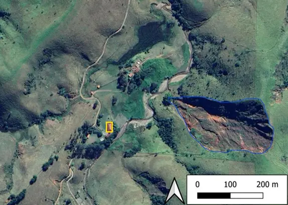
Figure 1. Aerial view of the study area located in the Vila Bom Jardim neighborhood, municipality of Bananal (SP). The yellow line indicates the affected residence, and the blue line highlights the gully located near the residence. Source: Image adapted by the author from Google Earth, 8 January 2025.
2. Materials and Methods
2.1. Materials
For the modeling, topographic and rainfall data, as well as land use and land cover information, were used to construct a representation of the water dynamics of the study area. The modeling was carried out using different software programs. The modeling was based on a Digital Elevation Model (DEM) from NASA, extracted from the USGS (United States Geological Survey) website. This DEM was used to identify the topographic features of the study area, enabling the visualization and analysis of slope, watershed divides, drainage lines, and potential areas of surface water accumulation. The data were initially processed in QGIS Desktop software, version 3.34.11, which allowed the generation of contour lines and the delimitation of the watersheds and sub-watersheds of interest. In addition, the Hidroflu program was used to determine the boundary conditions of the watershed. For the application in Hidroflu, data such as the length of the Bananal River within the study area (in km), the total drainage area (in km2), the average slope (m/m), the difference in elevation between the highest point and the basin outlet (in m), and the vegetation cover coefficient of the region were entered. The Excel program was also used for rainfall calculations for the models.
The field survey was conducted to collect in situ data for analysis of the study area. Equipment and materials were used to ensure efficiency and safety during the activities. These included a shovel and a pickaxe, used for excavating sampling points, and a measuring tape, used to measure depths and distances in the terrain. The location of the sample collection was identified using a GPS device (GPSMap 76CSx, Garmin Ltd., Olathe, KS, USA). A field activity was carried out where soil samples were collected and placed in raffia bags, which provide resistance and ease of transport by car to the laboratory.
A field activity was also carried out to obtain a more detailed, high-resolution terrain model through an aerial photogrammetric survey using a drone. The equipment used was a drone (Mavic 3, Enterprise, DJI, Shenzhen, China) equipped with an RTK sensor, which has the capacity to perform automatic flights, capture high-resolution images, and perform precise georeferencing of the images using GNSS (Global Nagivation Satellite System) receivers, a device that functions as an extremely precise and global GPS, capturing signals from satellite navigation systems to calculate its exact position (latitude, longitude and altitude) on the Earth’s surface. In addition, the Agisoft Metashape program was used to transform the drone images into contour lines. Laboratory analyses were conducted with the objective of characterizing the physical-geotechnical properties of the soil samples collected in the field, determining parameters such as texture, plasticity, moisture content, and density, which are essential for understanding the hydromechanical behavior of the material. Additionally, a visual analysis of samples taken from the riverbed was performed, with an emphasis on their mineralogical and granulometric characteristics, aiming to identify the predominant composition of the sediments and their correlation with processes of fluvial deposition and transport. All tests followed the technical standards established by the Brazilian Association of Technical Standards (ABNT), ensuring standardization and reproducibility. The general characterization of the samples involved the use of a rubber-coated wooden mortar, an oven (brand XYZ, accuracy of ±1 °C), an analytical balance (model ABC, capacity of 0.001 g), and a set of sieves (ASTM/E series, ranging from 0.075 mm to 4.8 mm). The granulometric analysis was performed in accordance with ABNT NBR 7181 (2016) [17], employing the following equipment: oven (accuracy ±1 °C), analytical balance (0.001 g), dispersing apparatus (brand DEF, standard rotation of 12,000 rpm), glass graduated cylinder (capacity of 1000 mL), hydrometer (accuracy of 0.001 g/cm3), thermometer (±0.1 °C), digital stopwatch (±0.01 s), beakers, sedimentation tank, sieve shaker (standardized rotation), glass rod, wash bottle, and metal capsules. The accuracy of the balance and hydrometer was decisive for obtaining a reliable granulometric curve, directly influencing soil classification and the estimation of parameters such as d90, used in the calculation of Manning’s coefficient.
The liquid limit test was performed according to ABNT NBR 6459 (2016) [18], using the following equipment: oven (±1 °C), porcelain dishes, steel spatula, Casagrande apparatus (with a standardized drop of 1 cm), steel grooving tool, and analytical balance (0.001 g). The precision of the Casagrande apparatus and the balance is critical for accurately determining moisture content at the transition point between the liquid and plastic states, a fundamental parameter for predicting soil behavior under saturated conditions. For the plastic limit test, in accordance with ABNT NBR 7180 (2016) [19], the following were used: porcelain dish, spatula, analytical balance (0.001 g), 3 mm diameter and 100 mm length cylinder (dimensional tolerance as per standard), and a ground glass plate (dimensions 30 cm × 30 cm). The dimensional precision of the cylinder and the sensitivity of the balance impact the determination of the moisture content at which the soil loses its plasticity, influencing classification and the prediction of deformations under load. The compaction test was conducted according to ABNT NBR 6457 (2016) [20] and NBR 7182 (2016) [21], employing the following materials: rammer (mass and dimensions standardized), large metal cylinder (standard volume of ≈2000 cm3), glass graduated cylinder, steel ruler (accuracy of 0.5 mm), analytical balance (0.001 g), oven (±1 °C), metal dishes, knife, sample extractor, metal tray, and plastic bag. The accuracy of the balance and compaction cylinder is essential for the reliable determination of maximum density and optimum moisture content, key parameters for assessing soil erosion susceptibility and infiltration capacity.
2.2. Methods
The hydrological and hydrodynamic modeling of the study area was carried out considering two main sources of topographic data: the Digital Elevation Model (DEM) provided by NASA; and a high-resolution DEM generated through aerial photogrammetric surveying with a drone. For both topographies, different computational packages were used for data processing, simulation, and analysis. In the first stage, the NASA DEM was inserted into the QGIS Desktop software (version 3.34.11) for delineation of the watershed. To carry out the hydrological modeling, the Bananal River watershed was initially delineated within the study area. After delineation, the DEM was used to generate a TIFF image with a resolution of 50 m square cells. These raster files were then converted to text files, formatted according to the requirements of the MODCEL software, for use in that program. In MODCEL, the initial project conditions were defined, such as the simulation time interval, the number of intervals, and the number of subdivisions. The Flow Cell Model is based on dividing the study area into homogeneous compartments, interconnected by hydraulic relationships that simulate the exchange of flows between them [22]. Although it uses one-dimensional equations, the model can represent flow in multiple directions in two-dimensional space. Raster models can be interpreted as Quasi-2D representations, which reinforces the suitability of MODCEL to this type of approach [23]. Manning roughness and surface runoff coefficients were assigned to each raster cell, based on analyses of satellite images, information on land use and land cover, and previously obtained morphometric parameters. The land-use classification enabled the identification of areas with varying infiltration capacities, including pastures, agriculture, riparian forests, and degraded areas. The Manning coefficient values were initially defined based on technical literature and refined based on the results. The hydrological simulation was fed with rainfall data from the Bananal meteorological station, considering critical events with a 25-year recurrence, as this period represents a condition of intense rainfall with a moderate probability of occurrence, making it suitable for assessing the vulnerability of the area and for designing mitigation measures compatible with the local reality. This data was used to generate rainfall scenarios based on the intense rainfall equation provided by the Hidroflu software, simulating concentrated precipitation over 24 h.
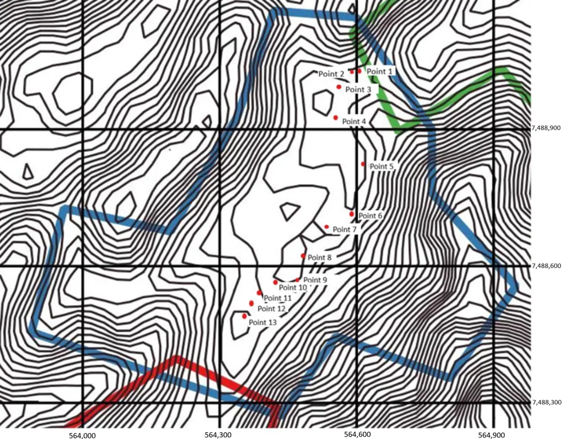
During the field survey, 13 distinct points along the riverbed within the property were identified and analyzed. Of these points, the first five were selected for soil sampling, aiming to provide a more detailed characterization of the physical and hydraulic properties of the terrain, fundamental for hydrological modeling and the analysis of susceptibility to erosion and flooding processes. At the remaining eight points, the type of material presented characteristics similar to those of the first five, so to avoid testing soil samples with similar properties, a comparative method was chosen for the five initially sampled points.
Samples were taken from the surface layer of the soil, up to 30 cm deep, and subsequently taken to the Geotechnical and Environmental Laboratory for geotechnical testing. Particle size analysis by sieving and sedimentation was conducted, in addition to the determination of hygroscopic moisture, in accordance with the technical standard NBR 7181 (ABNT, 2016) [17], which establishes the procedures for particle size analysis of soils. Based on the data obtained, particle size distribution curves were developed for the five samples, which are fundamental for characterizing soil behavior with respect to infiltration and permeability. Constructing these curves requires obtaining the mass of soil retained on each sieve or sedimented fraction, from which the cumulative passing percentage is calculated as a function of the equivalent particle diameter. Plotting this data on a semi-logarithmic scale (with the diameter on the logarithmic scale and the passing percentage on the arithmetic scale) yields the particle size distribution curve, which allows the soils to be classified according to their uniformity and the degree of particle dispersion. Based on the obtained particle size distribution curves, it was possible to determine the type of soil present in each of the samples. Furthermore, it was possible to calculate the d90 value for each sample, which corresponds to the effective diameter below which 90% of the particles by mass are found. This parameter is particularly relevant in geotechnical engineering and hydrology, as it relates to soil permeability and infiltration capacity.
The five graphs resulting from the particle size analysis, as well as their respective interpretations, are presented below in the graphs (Figure 2, Figure 3, Figure 4, Figure 5 and Figure 6) that follow.
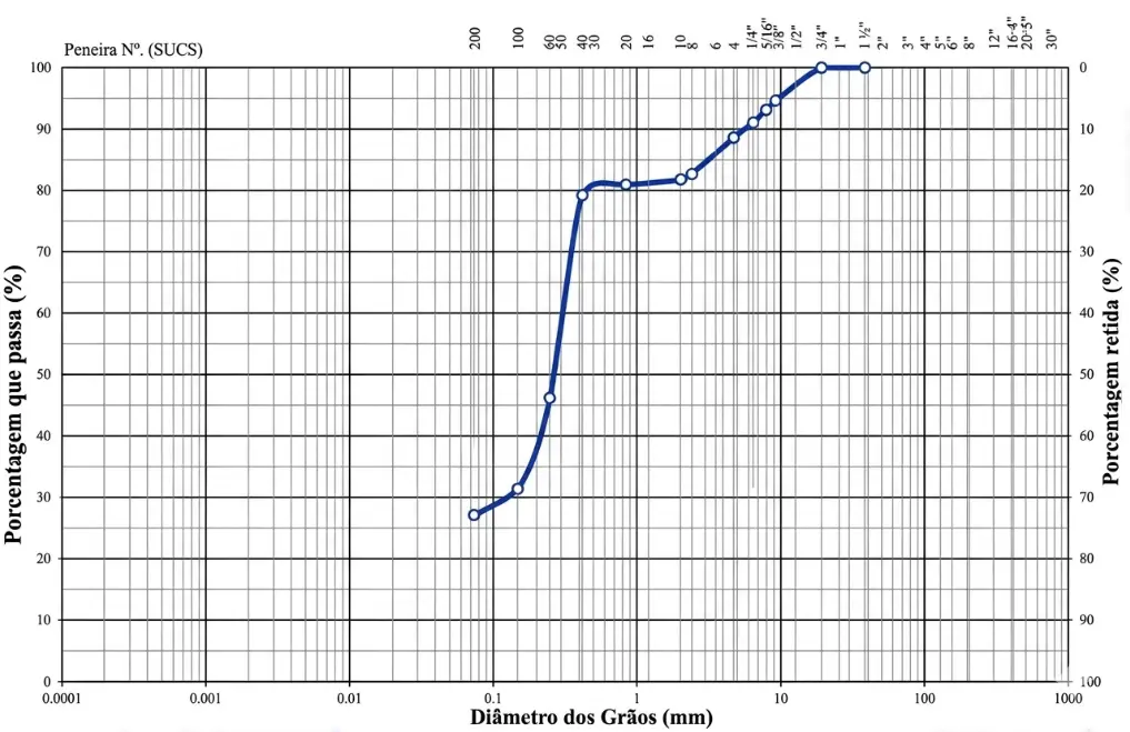
Figure 2. Particle size distribution curve of soil sample 1 indicating a well-graded sand. Source: Author, 2025.
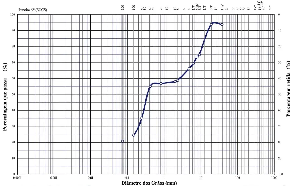
Figure 3. Particle size distribution curve of soil sample 2 indicating poorly graded sand. Source: Author, 2025.
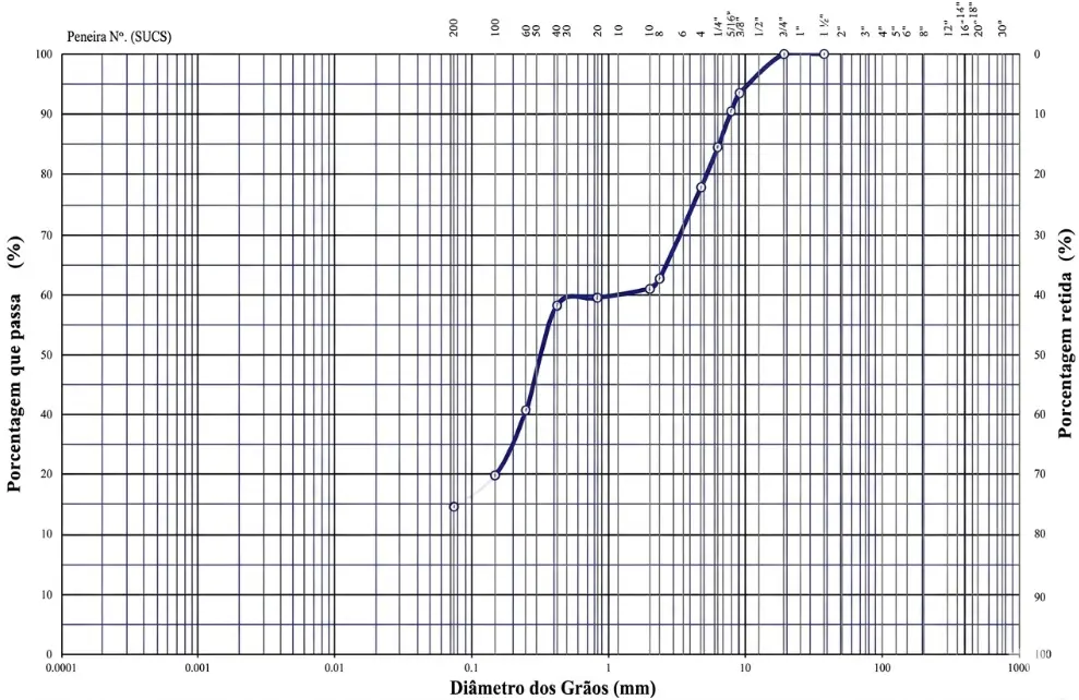
Figure 4. Particle size distribution curve of soil sample 3 indicating poorly graded sand. Source: Author, 2025.
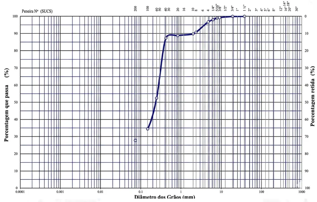
Figure 5. Particle size distribution curve of soil sample 4, indicating a well-graded sand. Source: Author, 2025.
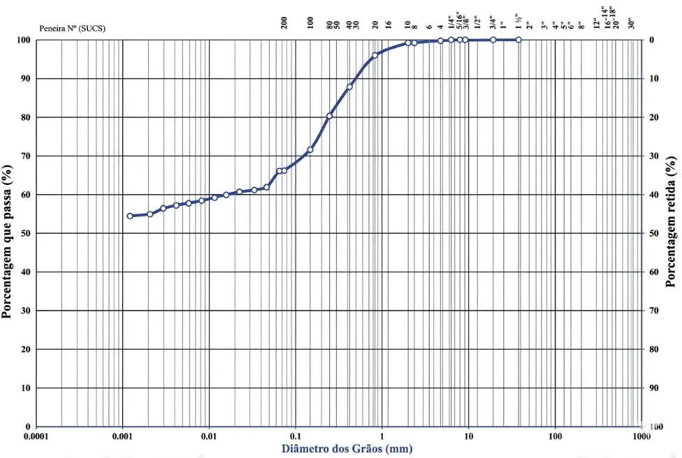
Figure 6. Particle size distribution curve of soil sample 5, indicating a well-graded sand. Source: Author, 2025.
On the second day of fieldwork, a high-resolution topographic survey was conducted using aerial photogrammetry with a DJI Mavic E3 drone equipped with a GNSS system for precise georeferencing. Before the flight, the area of interest was delimited in Google Earth software, encompassing both the area of the large gully located on the rural property and the sections where soil samples were collected. A kmz file was generated with the boundaries of the area to be overflown, which was transferred to the drone’s navigation system for automatic flight execution. To improve the positional accuracy of the captured images, a differential correction technique was applied using the Brazilian Network for Continuous Monitoring of GNSS Systems (RBMC), managed by the Brazilian Institute of Geography and Statistics (IBGE). The nearest identified station was RJRE0, whose data was then used to perform post-processing of the images, resulting in coordinates with centimeter accuracy. The images captured by the drone were processed in Agisoft Metashape software, where the three-dimensional surface model and contour lines of the mapped area were generated. The contour lines were then exported to QGIS, where a DEM corresponding to the area covered by the survey was created, representing only a part of the watershed delimited in the previous step. This high-resolution DEM was subsequently converted into a text file and exported to the MODCEL software, following the same methodology applied to the NASA DEM. However, since it was a small area of the watershed, a direct rainfall input was not used. Instead, a specific boundary condition was adopted, calculated from the modeling of the entire watershed performed with the first DEM. For this, the Hidroflu 2.0 software was used, with the following parameters: length of the main river (5.2 km), drainage area (6.95 km2), average slope (0.167 m/m), difference in elevation between the highest point and the outlet (868 m), and vegetation cover coefficient of the watershed (0.99). The boundary condition was entered as input data in MODCEL, allowing the simulation of hydrological behavior only in the portion of the basin represented by the drone survey. The model was run again with resolutions of 30 m and 10 m, in order to allow a future comparison between the results obtained with the NASA DEM and with the high-resolution DEM, generated specifically for the area of interest. Navigation and recording of the analyzed points were performed digitally, using the Avenza Maps application, which enabled the precise location of points of interest through the overlay of the reference map and GPS tracking. To ensure greater accuracy in determining geographic coordinates, a GPS device was used.
The map presented in Figure 7 was created based on the analysis of topographic images and Digital Elevation Models (DEMs), and shows points 1 to 13 of the field analysis. First, three areas were delimited, colored green, red, and blue, corresponding to sections of greatest interest for this work. The area delimited in blue corresponds to the region where soil samples were actually collected. The area delimited in green could not be accessed because it was another private property, and it was not possible to obtain the owner’s authorization for entry and sample collection. The area highlighted in red presented a large drop in the riverbed (waterfall), which significantly hindered access and made it impossible to safely collect samples in that portion of the terrain.
Laboratory analyses were conducted to characterize the physical properties of soils collected in the field and to better understand the geotechnical behavior of the materials present in the study area. Five soil samples, collected manually using a shovel, were analyzed at a maximum depth of 30 cm. This depth was chosen because it corresponds to the surface layer of the soil, which is the most susceptible to erosion, surface runoff, and climatic variations such as heavy rainfall and periods of drought. The granulometric characterization of the samples, from the municipality of Bananal (SP), began with a complete granulometric analysis, conducted according to the normative procedures of NBR 7181 (ABNT, 2016) [17], which defines the guidelines for determining the particle size distribution of soils.
3. Results
The results obtained in this work begin with the delimitation of the watershed of the study area, carried out using the QGIS 3.40.10 software, supplemented by contour lines generated by NASA’s DEM, as shown in Figure 8 below.
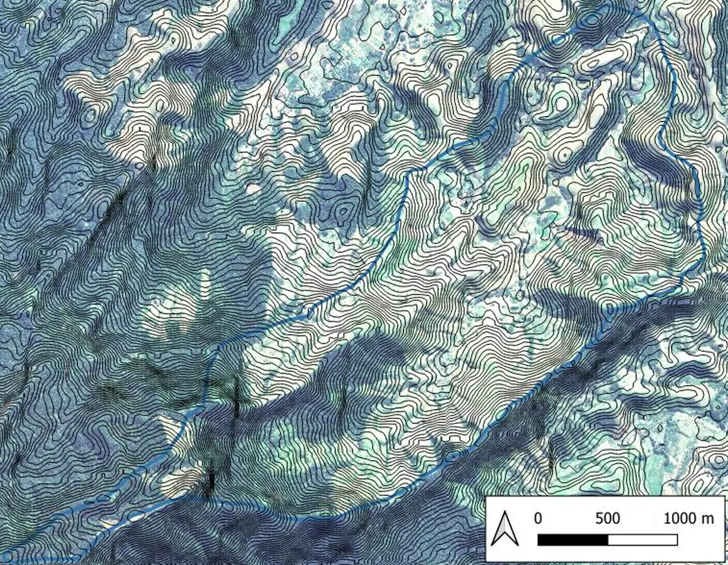
Figure 8. Basin delineated by contour lines generated by NASA’s DEM, using lighter colors. The blue boundary represents the limit of the watershed. Source: Author, 2025.
The first hydrodynamic model developed was based on a 50-m by 50-m grid, covering the entire extent of the basin. This initial model was built using QGIS software for export to MODCEL. Its structure had 2749 connected cells, representing the basin surface according to the topography extracted from NASA’s DEM. The initial conditions of the system were defined in this model, and precipitation data was inserted. It is worth noting that this model considered MODCEL’s internal hydrological modeling, using the rational method applied to each of the raster flow cells. The design rainfall used was calculated based on records from the Bananal meteorological station, considering a recurrence interval of 25 years, suitable for simulations of extreme events with high impact potential. Rainfall intensity was obtained using the IDF (Intensity–Duration–Frequency) equation formula, which relates precipitation intensity to its duration and frequency of occurrence. This equation is specific to each location and was applied here with the following parameters: a = 4.0477, b = 11.3018, c = 9.6083, d = 26.8795 and o = 0.6. These parameters were statistically derived using the Gumbel distribution applied to the annual maximum series, processed in Microsoft Excel with validation through the Anderson–Darling goodness-of-fit test. The temporal distribution of rainfall followed the alternating block method, discretized into 10-min intervals over a 24-h duration, consistent with the concentration time of the basin. The precision of the rainfall input is directly tied to the instrumental accuracy of the pluviograph (±0.1 mm) and the statistical uncertainty of the IDF parameters, estimated through a Monte Carlo simulation, resulting in a confidence interval of ±12% for intensity estimates in a recurrence interval of 25.
|
```latexi = \left(\frac{a}{{\left(t+b\right)}^{c}+d}\right)×o``` |
|
|
```latexi =\left(\frac{4.0477}{{\left(t+11.3018\right)}^{9.6083}+ 26.8795}\right)× 0.6``` |
The same precipitation parameters were used in all models developed based on NASA’s DEM. In addition, initial conditions regarding land use and surface runoff were included. Each cell was assigned a surface runoff coefficient, representing the soil’s infiltration capacity and the amount of water flowing superficially. The Manning coefficients adopted were 0.03, 0.04, 0.05, 0.055, 0.065, and 0.08, which were defined according to the surface characteristics of each area, from regions with stabilized beds to zones with dense vegetation, which directly influence the water flow velocity between cells. This variation allowed for differentiation of the hydrological behavior of regions with greater vegetation cover compared to areas more susceptible to runoff. A total of 5318 hydraulic connections were made between the cells. Based on these parameters, the model considered a flooding area of 0.5 m. This area was inserted to represent the river and the behavior of the water level in cases of overflow, allowing the simulation of floods in adjacent areas. The image generated by the model demonstrates the areas prone to flooding and highlights the importance of the spatial variation of the parameters for understanding the hydrological behavior of the basin. This model is represented in the following Figure 9.
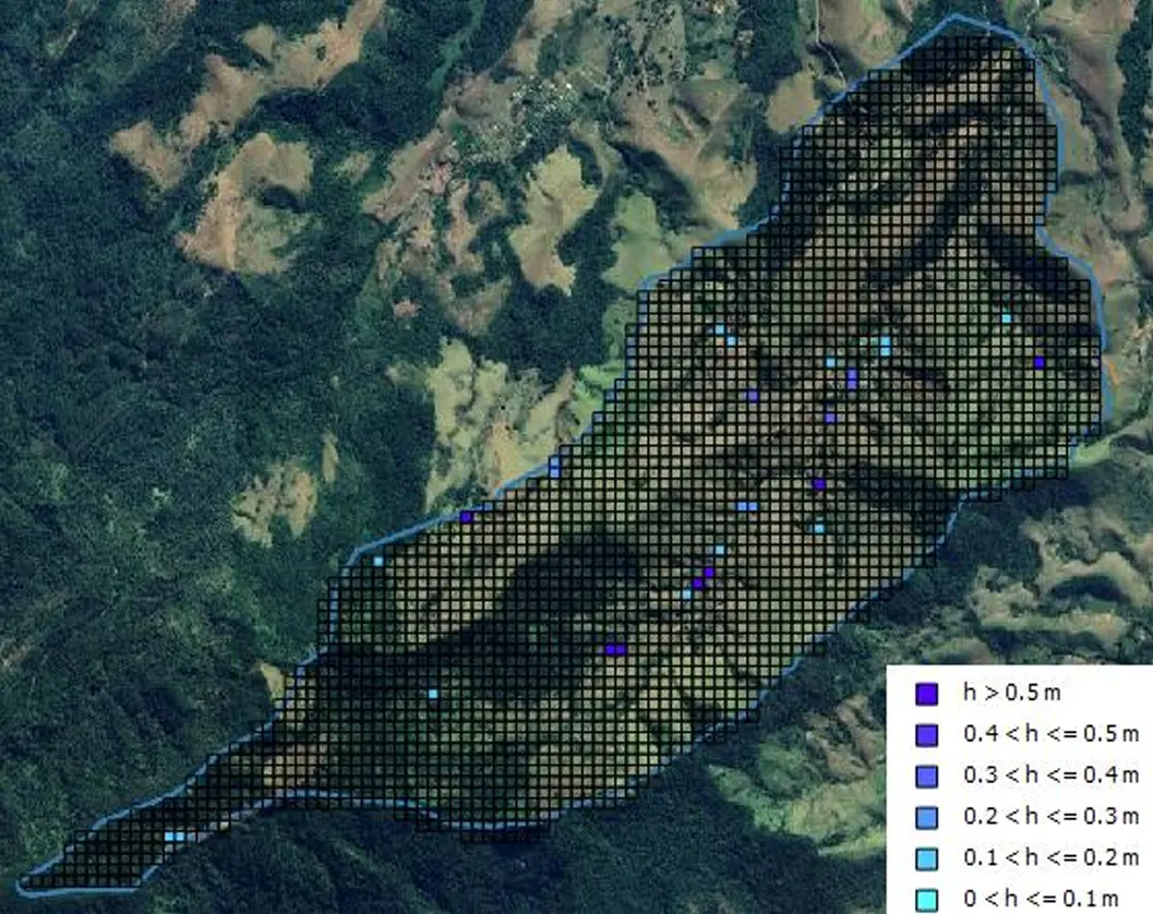
Figure 9. Model 1 and the flooded area up to 0.5 m created by the MODCEL program. Source: Author, 2025.
The second hydrodynamic model developed in this work also used MODCEL and followed the same precipitation pattern adopted in the first model, calculated based on the IDF (Intensity-Duration-Frequency) equation. As in the previous model, NASA’s Digital Elevation Model (DEM) was used to represent the relief of the study area. This model maintained the 50-m resolution cells, totaling 2749 cells. The same runoff coefficients adopted in Model 1 were maintained in this model: 0.00, 0.35, 0.40, and 0.55, as well as the Manning roughness coefficient values. The difference between Models 1 and 2 lies in the definition of the connections between river sections and their banks. In Model 2, diagonal connections were introduced in regions where flow was possible, allowing for flow exchange between cells connected also by the vertices of the raster cells. This adjustment provides a more accurate representation of the region’s different flow dynamics. A simulation of the flood zone was performed, considering a depth of up to 0.50 m, which allowed for a better visualization of potentially flooded areas. The results obtained from this modeling are presented in Figure 10 below.
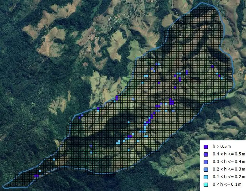
Figure 10. Model 2 with 50 × 50 m cells and flooding area up to 0.5 m created by the MODCEL program. Source: Author, 2025.
Model 3 was also developed from NASA’s Digital Elevation Model (DEM); however, unlike previous models, this one was created with a more refined spatial resolution, using 30-m cells. This scale was chosen in the expectation that surface runoff would be represented more accurately, allowing for a more detailed capture of the basin’s topographic variations and, consequently, the flow dynamics. This model was structured in two distinct stages. The entire watershed was subdivided into 7914 regular 30 × 30-m cells, to which a uniform surface runoff coefficient of 0.18 was assigned. As for the Manning roughness coefficient, a constant value of 0.03 was adopted for all cells in the basin. In this initial stage, no spatial variations were introduced into the Manning coefficient. As a result of this configuration, the following hydrodynamic behavior was obtained, as shown in Figure 11.
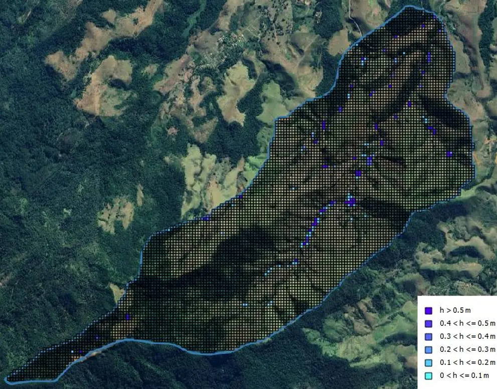
Figure 11. Model 3 with 30 × 30 m cells and flooding area up to 0.5 m created by the MODCEL program. Source: Author, 2025.
Model 4 represents the most refined version of the simulation, developed based on a spatial resolution grid of 30 m, totaling 7914 cells distributed throughout the watershed. This model incorporated field data obtained through soil sampling at five points in the study area, located in the municipality of Bananal (SP).
After conducting particle size analysis in the laboratory, using soil samples collected during fieldwork in Bananal (SP), particle size distribution curves were created for each sampled point. With the aid of Excel 2016 software, it was possible to interpolate the obtained data and determine the d90 value for each of the curves. This parameter corresponds to the sieve diameter that allows 90% of the soil by mass to pass through. Determining d90 is essential for applying the empirical formula proposed by Meyer-Peter and Müller (1948), which allows estimating the Manning roughness coefficient (n) based on the particle size distribution characteristics of the soil. The calculations performed using this formula, as well as the values obtained for each point analyzed, are presented in Table 4 below.
Table 4. Manning’s coefficient is calculated from the d90 values found in the Particle Size Distribution Curve.
|
Meyer-Peter Equation |
|||
|---|---|---|---|
|
n = 0.038 × d901/6 |
|||
|
d90 |
N |
Sample |
|
|
P1 |
5.6781 |
0.05075561597 |
Well-Graded Sand (SW) |
|
P2 |
17.1493 |
0.06102268737 |
Poorly Graded Sand (SP) |
|
P3 |
7.8068 |
0.05352160216 |
Poorly Graded Sand (SP) |
|
P4 |
2.0946 |
0.04298336844 |
Well-Graded Sand (SW) |
|
P5 |
0.5328 |
0.03421456052 |
Well-Graded Sand (SW) |
Furthermore, Model 4 incorporated the equation proposed by Ven Te Chow (1959) to estimate the Manning coefficient in rural areas, such as pastures and areas with sparse housing, as well as in stretches of dense forest. This approach allows for a more comprehensive assessment of flow resistance in longer stretches, where additional variables, besides the channel lining material, influence flow behavior.
This calculation is shown in Table 5 below.
Table 5. Manning’s calculation for the forest area and rural area from the Vem te Chow equation.
|
Ven te Chow Equation |
|||||||
|---|---|---|---|---|---|---|---|
|
n = (n0 + n1 + n2 + n3 + n4) × m5 |
|||||||
|
n0 |
n1 |
n2 |
n3 |
n4 |
m5 |
N |
|
|
Forest |
0.025 |
0.05 |
0 |
0.019 |
0.025 |
1 |
0.119 |
|
Rural |
0.025 |
0.05 |
0 |
0.005 |
0.01 |
1 |
0.09 |
Therefore, for the construction of Model 4 in this study, different values of the Manning coefficient were used according to the specific characteristics of each area. The cells corresponding to sampling points 1 to 5 received individualized n values, determined based on the analysis of the particle size distribution curve of the soils collected in the field, as shown in Table 4 and Table 5. The other areas of the model, such as the rural zone and the stretches with dense forest cover, were assigned specific Manning values calculated from the equation proposed by Ven Te Chow (1959), as shown in Table 3.
In this way, Model 4 has a more refined spatial variation of the hydraulic roughness parameter, increasing the reliability of the surface flow simulation.
Figure 12 shows how these values are applied in the modeled space.
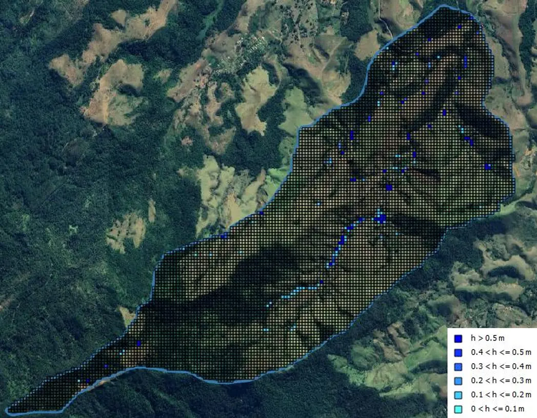
Figure 12. Model 4 with 30 × 30 m cells that used different specific Manning coefficients added to the flood area up to 0.5 m carried out by the MODCEL program. Source: Author, 2025.
Model 5 was developed differently from the previous ones. Instead of using the design rainfall as input data, the river flow was calculated beforehand using the Hidroflu 2.0 program. This flow was then inserted into a raster cell upstream of the area of interest representing the riverbed, with the aim of simulating the hydrodynamic behavior of the watercourse in response to this volume. This procedure was adopted to verify whether the delimitation and modeling of the entire watershed would, in fact, be indispensable for obtaining reliable results in the simulation of floodable areas. Furthermore, this approach allowed for direct comparison with Models 7 and 8, which used a Digital Elevation Model (DEM) obtained by drone without resorting to complete hydrological modeling of the main basin. In this way, the aim was to understand whether the use of high-resolution data and a more restricted spatial scope would be sufficient to reproduce the hydrodynamic behavior of the river in flood scenarios. To calculate this flow rate, the Hidroflu 2.0 software was used, which estimates surface runoff flow from morphometric and hydrological parameters of the sub-basin in question. The following data was entered into Hidroflu: length of the main river (Bananal River), measured at 5.2 km; contributing drainage area, estimated at 6.95 km2; average slope of the watercourse, of 0.167 m/m; difference in elevation between the highest point and the outlet, of 868 m; and the vegetation cover coefficient, adopted as 0.99. In addition, precipitation and land use/land cover data were used to calculate the inflow rate. After defining the inflow rate using Hidroflu, a cell corresponding to the riverbed was manually selected. This cell represents the initial point of surface flow within the modeled area and serves as the upstream boundary condition. With this cell defined and the flow values entered, it was possible to properly configure the flow in MODCEL. Next, the area potentially subject to flooding was delimited, adopting as a criterion a water depth of up to 0.5 m. This delimitation allowed the identification of the most vulnerable zones to flooding within the study area, resulting in the final map presented below, which shows the simulated flooding dynamics in Model 6. This model is shown in Figure 13. This model used NASA’s Digital Elevation Model (DEM), with a spatial resolution of 30 m per cell. In this model, the Manning’s Roughness coefficient was 0.03, and the runoff was 0.18; however, these values were not very relevant to the model since the river flow was used.
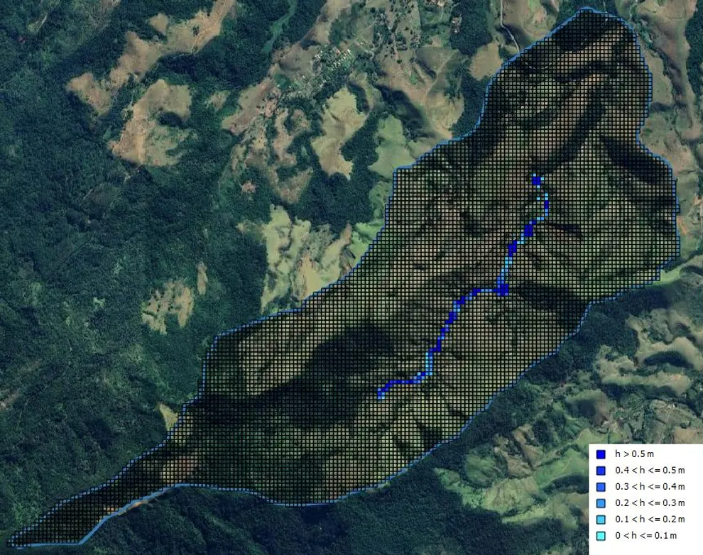
Figure 13. Model 5 with 30 × 30 m cells that used different specific Manning coefficients added to the flooding area up to 0.5 m performed by the MODCEL program. Source: Author, 2025.
Model 6 was developed from a DEM (Digital Elevation Model) generated based on contour lines obtained through a topographic survey conducted with a drone during fieldwork. The activity was conducted in a single day, requiring approximately one hour for equipment preparation and another hour of drone flight for data collection. The survey resulted in coverage of approximately 0.87 km2 of mapped area. Figure 14 shows the generated DEM, highlighting the contour lines and their respective altitudes, which allowed for a representation of the relief of the study area.
The grid used in the modeling, with its respective dimensions and spatial boundaries, is shown in Figure 15.
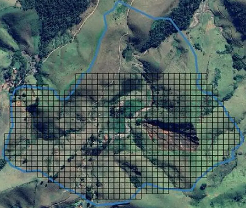
Figure 15. Delineation of the area where the drone topographic survey was carried out, marked with 30-m cells. Source: Author.
This model 6 had a total of 968 cells. The Manning’s Roughness coefficient was 0.03, and the runoff coefficient was 0.18; however, these runoff values were not as relevant to the model, as the river flow previously calculated by Hidroflu in Model 5 was used. This model, representing only a section of the watershed, also used river flow as input data rather than design rainfall. The same flow values previously calculated in the Hidroflu program and applied in the previous model were used. Next, the area potentially subject to flooding was delimited, using a water depth criterion of up to 0.5 m.
This delimitation allowed the identification of the most vulnerable zones to flooding within the study area, resulting in the final map presented below, which shows the flooding dynamics simulated in Model 6. This model is shown in Figure 16.
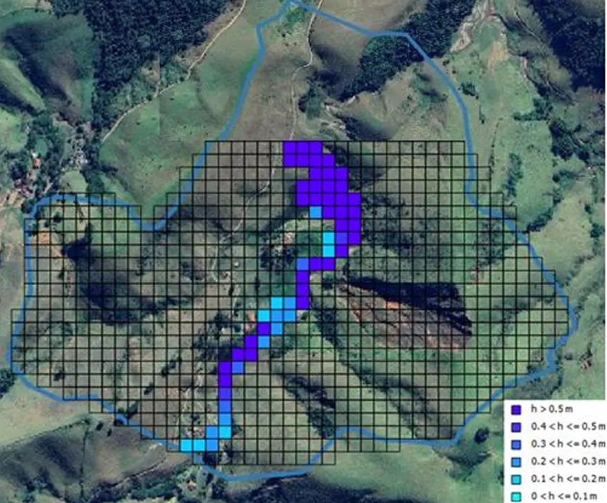
Figure 16. Model 6 with 30 × 30 m cells added to the flooding area up to 0.5 m, created by the MODCEL program. Source: Author, 2025.
Model 7, developed in this work, was also based on the Digital Elevation Model (DEM) generated from the drone topographic survey. However, unlike Model 6, which used a spatial resolution of 30 m, this model was refined by adopting 10-m cells. The objective of this higher resolution was to improve the representation of the relief and, consequently, obtain more precise results in the surface runoff simulation. The same hydrodynamic parameters applied in the previous model were maintained.
The boundary condition also remained the same, using the inflow calculated in Hidroflu based on the hydrological characteristics of the sub-basin. With the new resolution, the model now has 8615 cells, allowing for a more detailed analysis of the distribution and behavior of the water depth in the study area. As with the previous models, a flood depth of up to 0.5 m was considered, allowing for the visualization of potentially floodable areas. The final simulation result is shown in Figure 17 below.
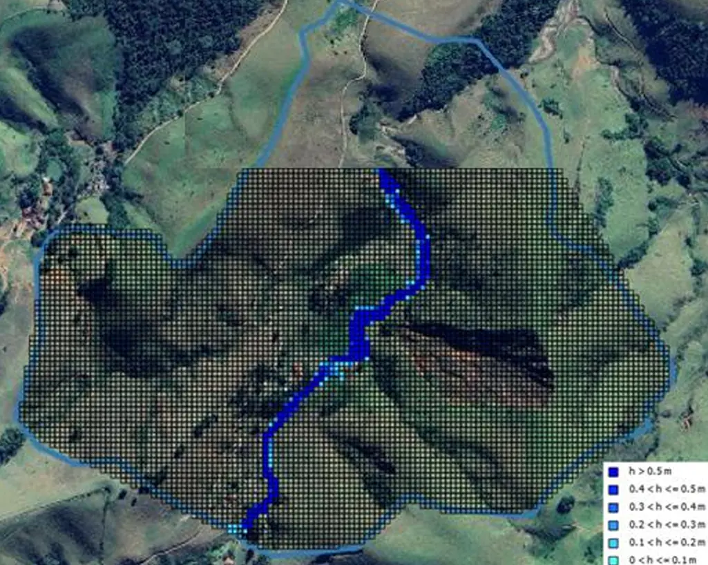
Figure 17. Model 7 with 10 × 10 m cells added to the flooding area up to 0.5 m, created by the MODCEL program. Source: Author, 2025.
4. Discussions
To begin the discussion of the results obtained, it is important to highlight a fundamental difference between the models analyzed in this study: the spatial extent of the modeling area. While Models 1 to 5 used a Digital Elevation Model (DEM) derived from NASA data, covering the entire watershed with a total area of approximately 6.96 km2, the DEM used in Models 6 and 7 was obtained from a drone topographic survey, covering a significantly smaller area of about 0.82 km2. This represents a reduction of approximately 88.2% in the modeled area when using the drone-derived DEM. This substantial difference in spatial coverage, visually represented in Figure 18, is a critical factor to consider when comparing model outputs and their respective resolutions, as it directly influences the scale of analysis and the detail captured in the hydrodynamic simulations.
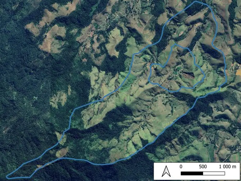
Figure 18. The difference between the modeled areas in the two sets of simulations allows a clear visualization of the spatial delimitation adopted in each approach. Source: Author, 2025.
Thus, when comparing the results of the models, it is observed that Models 1 and 2, made from NASA’s DEM and using 50-m cells, presented significant limitations in terms of spatial resolution. Although both models identified a flooding zone between the gully and the house area, the representation of this area was not very detailed, which compromises the interpretation of the real impacts on the landscape. Even with the variation in Manning’s roughness coefficient between the two models, the improvement in the definition of the flooded areas was neither substantial nor visibly clear. This suggests that, in addition to hydraulic parameters, model resolution plays a fundamental role in the quality and reliability of the simulations, especially in critical areas where small topographic variations can significantly alter flow patterns.
Figure 19 shows the difference between these two models.
 |
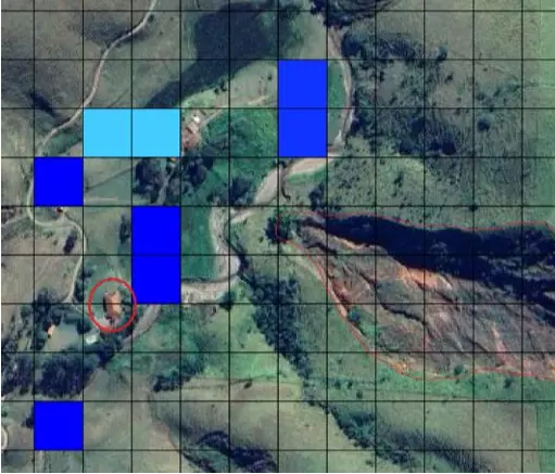 |
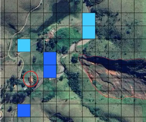
Figure 19. Differences in the area of greatest interest between models 1 and 2. Darker blue shades represent areas of greater flood extent, while lighter blue tones indicate lower levels of inundation. The gully located near the property is highlighted with a thin red line, and the property most affected in the map is marked with a thick red circle.
Models 3 and 4 showed a higher level of refinement compared to the previous ones, as they used 30-m cells, the lowest possible resolution based on NASA’s DEM. This improvement allowed for a more detailed representation of the hydrological processes in the study area. In Model 3, the flooded area located between the residence and the gully became more visible, coinciding with the reports from the site’s residents, who indicate this region as one of the most affected by flooding. However, Model 4, which sought to further refine the results by applying Manning’s coefficients adjusted based on specific laboratory analyses of the area, did not show significant improvements compared to the previous models that used coefficients extracted from the literature. This result suggests that, in this case, the spatial resolution and the model structure had a greater influence on the quality of the simulation than the fine adjustments to the hydraulic parameters of Manning’s roughness coefficient and surface runoff coefficient. The results of these three models are summarized in Figure 20 below.
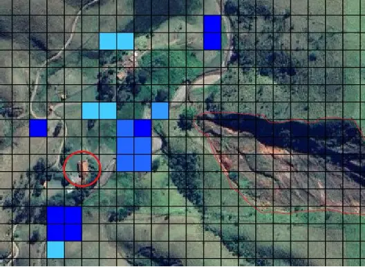 |
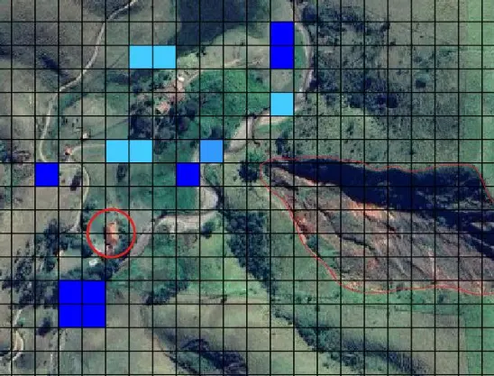 |
Figure 20. Differences in the area of greatest interest between models 3 and 4. Darker blue shades represent areas of greater flood extent, while lighter blue tones indicate lower levels of inundation. The gully located near the property is highlighted with a thin red line, and the property most affected in the map is marked with a thick red circle.
The lower precision observed in Model 4 may be related to the methodology used to calculate Manning’s roughness coefficient. This model adopted the Meyer-Peter and Müller equation is indicated for situations where the riverbed is composed, in a significant proportion, of coarse material, i.e., sediments such as gravel, pebbles, and blocks, whose granulometry is considerably larger than that of sands and silts. However, it is possible that this condition does not apply to the study area, which may predominantly have clayey or sandy soils or soils covered by vegetation, without a significant presence of coarse material. Thus, the application of this empirical model may have led to Manning’s values that do not adequately represent local reality, thereby compromising the accuracy of the hydrological model. Furthermore, in Model 4, the Manning coefficients calculated for the rural and forest areas were calculated using Cowan’s method, which consists of the weighted sum of six factors: type of bed material, degree of surface irregularity, variation in cross-section, presence of obstructions, vegetation present, and degree of meandering of the watercourse. Although the method is widely used and recognized, it strongly depends on visual and subjective interpretation in the field, which can introduce evaluation errors, especially in areas with dense vegetation, low visibility, or restricted access.
Given that the main flooding zone lies between the residence and the gully, according to residents’ reports, it is likely that Model 4, which used Manning coefficients directly extracted from specialized literature, provided a more faithful representation of reality. Manning’s Roughness Coefficients were obtained from the document “Guide for Selecting Manning’s Roughness Coefficients for Natural Channels and Flood Plains”, published by the United States Geological Survey (USGS), Water-Supply Paper 2339, authored by George J. Arcement Jr. and Verne R. Schneider, which has been widely used as a technical reference in hydrological and hydraulic modeling.
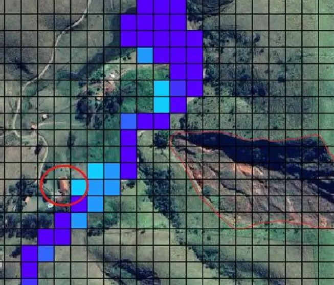
Model 5, on the other hand, used the river flow rate, previously calculated using the Hidroflu software, as input data instead of the design rainfall adopted in previous models. As expected, this model produced different results, providing a more realistic representation of flow behavior along the main channel of the Bananal River. It was possible to observe, with greater clarity, the recurrence of flooding in the area located between the residence and the gully. This approach proved more effective in identifying critical flooding points compared to the direct use of precipitation in MODCEL. However, it is important to highlight that the river flow rate estimated by Hidroflu itself is dependent on several hydrological factors, including precipitation with a 25-year recurrence interval, the same adopted in previous models, as well as other sub-basin-specific parameters such as the length of the main river (Bananal River), the contributing drainage area, the average slope of the watercourse, the difference in elevation between the highest point and the outlet, and the vegetation cover coefficient. In addition to these, the calculation also considered the runoff coefficient, the Curve Number (CN), and the beta coefficient, which directly influence the estimation of the surface runoff volume generated by rainfall. These elements make the obtained flow rate a more accurate representation, especially in critical areas subject to flooding. Therefore, we can say that, for this project, using the river flow rate as input data was more effective than directly applying the design rainfall, providing a simulation closer to the local reality. This representation is shown in Figure 21 below.
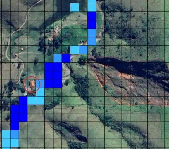
Figure 21. Analysis of the Bananal River flooding in model 5. Darker blue shades represent areas of greater flood extent, while lighter blue tones indicate lower levels of inundation. The gully located near the property is highlighted with a thin red line, and the property most affected in the map is marked with a thick red circle.
Models 6 and 7 were developed based on the Digital Elevation Model (DEM) generated by aerial photogrammetric surveying with a drone. Model 6, built with a spatial resolution of 30 m, presented results quite similar to Model 5, which had used the NASA DEM with the same resolution and the same flow values of the Bananal River, previously calculated by the Hidroflu software. This equivalence allows us to conclude that, in contexts where a high level of spatial detail is not required, the use of the NASA DEM proves adequate and efficient for applications in hydrological projects, considering that its maximum available resolution is 30 m. However, when the objective of the study requires greater precision, such as the analysis of specific critical areas or the observation of micro-reliefs and more detailed features, the use of high-resolution DEMs, such as those obtained by drone, is significantly more effective. This was evidenced in Model 7, which used 10-m cells derived from the same aerial survey. In this model, it was possible to observe with greater clarity the areas susceptible to flooding, especially the region between the gully and the residence, and to provide a more refined visualization of the riverbed curves. Therefore, it is concluded that Model 7 represents the most complete simulation among all those performed in this work. The images generated by this model clearly show the floodable areas, as reported by local residents, as presented in Figure 22.
In the specific context of this project, the use of a drone proved extremely useful, as it enabled the obtaining of a detailed DEM that allowed for a clearer observation of the river’s behavior, its curves, overflow points, and the areas most susceptible to flooding. This more precise visualization was essential to identify the critical zone between the gully and the residence.
 |
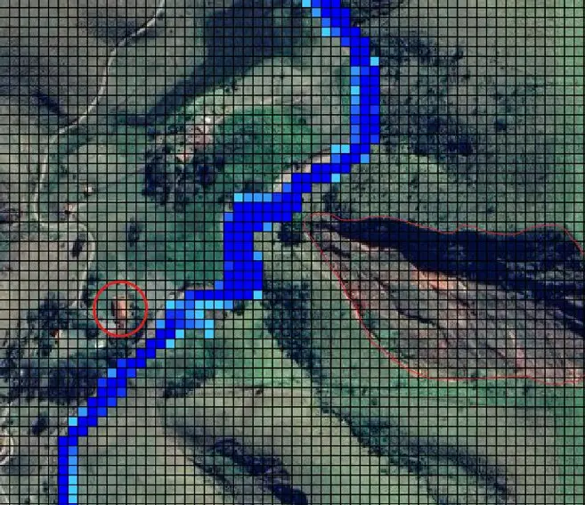 |
Figure 22. Differences between 10 m and 30 m cells with the DEM generated by drone. Darker blue shades represent areas of greater flood extent, while lighter blue tones indicate lower levels of inundation. The gully located near the property is highlighted with a thin red line, and the property most affected in the map is marked with a thick red circle.
It was observed that models with a larger number of cells required more processing time compared to those with fewer cells. In the case of the entire basin simulation, even using a 30 m grid, the time was significantly increased due to the inclusion of design rainfall in the model, as well as Manning’s coefficients and runoff parameters, which increased computational complexity. On the other hand, models in which the flow rate was directly inserted into a single cell showed slightly shorter times, although still proportional to the number of cells. It is noteworthy that Model 6, with the fewest cells, was faster, completing in less than an hour, while others, such as models 2, 4, 5, and 7, with a resolution of 10 m, took more than 8 h to process. This performance demonstrates that, for the efficient execution of work involving numerical modeling and highly complex spatial simulations, the use of a powerful processor and an adequate amount of RAM is fundamental to optimizing processing time. Table 6 shows the time required to run each of the models in MODCEL, allowing for an assessment of the impact of hardware configurations on simulation duration.
Table 6. Processing time for each of the eight models on the computer used to carry out this work.
|
Model Number |
Number of Cells |
Cell Size (In Meters) |
Approximate Duration (In Hours) |
|---|---|---|---|
|
1 |
2749 |
50 × 50 |
2 |
|
2 |
2749 |
50 × 50 |
2 |
|
3 |
7914 |
30 × 30 |
10 |
|
4 |
7914 |
30 × 30 |
10 |
|
5 |
7914 |
30 × 30 |
8 |
|
6 |
968 |
30 × 30 |
1 |
|
7 |
8615 |
10 × 10 |
8 |
The comparative analysis of the hydrodynamic models developed in this study allowed for a critical evaluation of the influence of spatial resolution, the source of topographic data, and the definition of boundary conditions on the simulation of flood-prone areas in rural basins. The results directly address methodological issues widely discussed in the literature, particularly regarding the trade-off between topographic detail, computational cost, and modeling accuracy. The significant difference in the representation of flooded areas between low-resolution (50 m) and high-resolution (10 m) models corroborates well-established findings in the literature. Studies such as those by Lim & Brandt (2019) [24] and Zhao & Chen (2021) [25] demonstrate that models with cells larger than 30 m tend to underestimate flood extent in complex terrains, as they fail to capture micro-depressions and flow barriers. In the present study, Models 1 and 2 (50 m, based on the NASA DEM) provided a generic, poorly detailed representation of the flood zone between the gully and the residence, limiting the usefulness of the maps for local planning. This result aligns with the observation by Miguez et al. (2017) [22], who, while employing MODCEL, emphasized the importance of DEMs with resolution compatible with the scale of the features of interest for realistic simulations. The equivalence of results between Model 5 (NASA DEM 30 m) and Model 6 (drone DEM 30 m) suggests that, at the same spatial resolution, the origin of the topographic data has a secondary impact on the overall delimitation of risk areas. This indicates that, in reconnaissance studies or for larger basins, the use of free orbital DEMs, such as those from USGS/NASA.
However, the quality leap observed in Model 7 (10 m, drone) reinforces the argument that high resolution is indispensable for detailed analyses. The clear identification of the river meander and the critical overflow zone near the house was only possible with the 10 m mesh, a fact widely documented in studies that employed UAVs for hydrological modeling. These authors emphasize that resolutions below 5–10 m are necessary to capture hydraulically relevant geometry in low-order channels, common in rural areas. The superiority of models that used estimated flow (Models 5, 6, and 7) over those based solely on design rainfall (Models 1–4) in representing the behavior of the Bananal River finds support in the technical literature. As discussed by Chow et al. (2013) [26], the rainfall-runoff transformation introduces additional uncertainties into the model, which depend on the accuracy of the loss parameters (runoff, CN) and the representation of flow propagation in the basin. In the context of this study, the runoff and Manning parameters, even when calibrated, may not have fully captured the spatial heterogeneity of the basin, leading to a less precise representation of the hydrograph. The approach of using an externally calculated inflow (with HidroFlu) simplified the model structure in MODCEL and produced results more consistent with residents’ reports.
The expectation that fine calibration of the Manning coefficient based on local granulometric analyses (Model 4) would bring significant improvements did not materialize. The results of Model 4 were similar to those of Model 3, which used tabulated values. This observation converges with the conclusions of Sanz-Ramos et al. (2021) [27], who point out that, in large-scale models (even with 30 m cells), sensitivity to roughness can be masked by other sources of uncertainty, such as topographic resolution and the simplification of flow processes. The Meyer-Peter and Müller method, used to estimate the Manning coefficient from d90, is recommended for beds with coarse material (Baptista, 2007 [28]). Its less effective application in this study may indicate that sediment transport and roughness in the area are more influenced by vegetation and terrain macro-roughness than by fine soil texture, a hypothesis that deserves investigation in future work. On the other hand, the successful use of Manning values from the technical literature (USGS, Arcement & Schneider, 1989 [29]) in Model 3 reinforces the usefulness of these established references in engineering studies, especially when detailed local data are scarce or prohibitively costly.
The exponentially longer processing time for high-resolution models (Model 7: 8 h) compared to low-resolution ones (Model 6: 1 h) highlights a crucial practical challenge. This relationship between resolution, number of cells, and computational demand is well known in environmental modeling and imposes a design decision: one seeks the greatest possible detail within the limits of available time and hardware. For risk management on rural properties, a model similar to model 7 may be justifiable for the final design of an intervention, while models similar to models 5 or 6 would be more suitable for diagnostic and planning stages. The contribution of this study lies in the empirical and comparative evaluation of these different approaches in a real case, quantifying gains in precision and costs in complexity. The findings reinforce the importance of a scalable and adaptive approach to hydrological modeling for rural planning, aligning with recent recommendations for integrating multi-data and multi-models in natural disaster management (Merz et al., 2020 [30]).
Therefore, the results obtained in this work show that the methodology adopted, using the MODCEL program, proved effective for the proposed modeling, achieving satisfactory results, especially when associated with the use of the Digital Elevation Model (DEM) obtained by drone. It is recommended to expand the use of the MODCEL software to conduct new studies that explore its potential across different contexts and basin types, thereby strengthening its consolidation in the academic and technical fields. Given the results and the analysis of local hydrological dynamics, it is evident that the region near the Santa Inês site faces problems due to flooding and overflows of the Bananal River. The erosive process in this area is constant, aggravated by the absence of adequate vegetation cover near the riverbeds and the lack of containment infrastructure. These occurrences negatively impact both the environment and local human activities, increasing soil degradation and siltation of water bodies.
Figure 23 shows a comparison between the three most representative hydrodynamic models obtained in this study. Model 5, shown on the left, and Model 6, in the center, indicate that the flood zone approaches the existing residence in the study area, although they do not clearly show the meander in the upper part of the river. Model 7 allows clearer identification of this feature and provides a more realistic simulation of flooding near the house. From this analysis, it is concluded that the configuration based on 10-m cells is the most suitable, as it guarantees better quality and precision in the representation of fluvial dynamics.
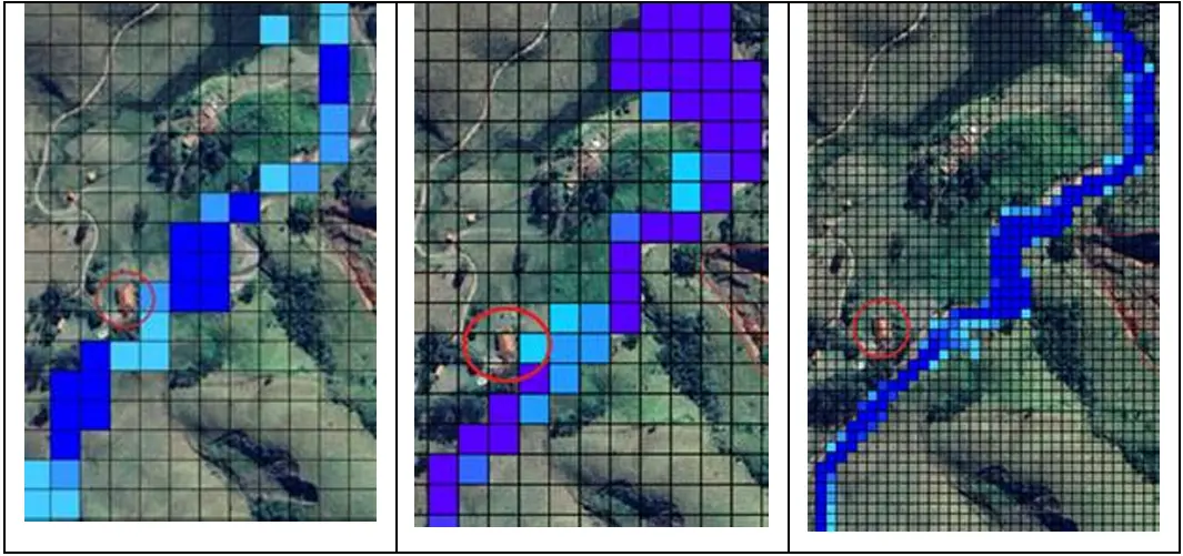
Figure 23. Models 5, 6, and 7, respectively, which were considered the most representative models. Darker blue shades represent areas of greater flood extent, while lighter blue tones indicate lower levels of inundation. The gully located near the property is highlighted with a thin red line, and the property most affected in the map is marked with a thick red circle.
5. Conclusions
Based on the analysis conducted, this study concluded that hydrodynamic modeling is an essential tool for understanding and managing floods in the rural area of Bananal (SP). The comparison of SEVEN models, developed with different spatial resolutions, sources of topographic data (NASA DEM and drone-based DEM), and boundary conditions (precipitation and flow), demonstrated that the use of estimated river flow as the main input produces more realistic results and is less sensitive to parametric variations, being the most recommended approach for the studied context. The use of a high-resolution DEM obtained by drone (10 m) allowed detailed mapping of critical flood areas, surpassing the accuracy of the 30 m orbital DEM, especially in identifying local features such as meanders and overflow zones. However, the costs associated with the drone and the higher computational demands limit its large-scale application or use in projects with limited resources. In these cases, NASA’s DEM proved to be a viable alternative for preliminary analyses. Hydraulic parameters derived from technical literature showed satisfactory effectiveness, suggesting that in contexts without major heterogeneities, field campaigns can be optimized. The main limitations of the study were the dependence on computational capacity for high-resolution simulations and the restricted spatial coverage of the drone survey. For future research, it is recommended to expand drone mapping, integrate artificial intelligence techniques for automated calibration, and apply the methodology to other rural basins, aiming to validate its replicability and improve evidence-based mitigation strategies.
A significant limitation of this study lies in the absence of formal validation of the hydrodynamic models against observed flood data, such as historical flood extents or high-water marks. The validation conducted was predominantly qualitative, based on “reports from the site’s residents”, which, while valuable for contextualizing the results, does not replace quantitative and objective verification. The exclusive use of these reports introduces subjectivity that may affect the robustness of the conclusions. Therefore, it is recommended that future work incorporate more robust validation methods, such as using satellite imagery of past events, high-precision post-event surveys, or comparisons with historical flow and flood-stage data. This approach would allow for more reliable calibration and verification of the models, enhancing the scientific rigor and practical applicability of the results for hydrological risk management.
Statement of the Use of Generative AI and AI-Assisted Technologies in the Writing Process
During the preparation of this manuscript, the author(s) used DeepSeek in order to assist with the translation of the article. After using this tool/service, the author(s) reviewed and edited the content as needed and take(s) full responsibility for the content of the published article.
Acknowledgments
The authors would like to express their sincere gratitude to the laboratory technicians at the Pontifical Catholic University of Rio de Janeiro for their valuable technical support. The authors also wish to thank Solonovo Soluções Sustentáveis, especially Julio Prezotti, José Márcio Ferreira and Lucas Bridi, for providing the drone used in this study and for their technical guidance on its operation. Special thanks are extended to Gabriel Nogueira Brum for his kindness in allowing this research to be conducted on his property, generously granting access to the study area, which was essential for the development of this work. The authors are also grateful to Roberto Newton Carneiro, from IBIOS, for his continuous support and for closely following all stages of this research. Finally, the authors would like to thank all those who contributed, directly or indirectly, to the completion of this study.
Author Contributions
Conceptualization, A.R.L.D.; Methodology, A.R.L.D.; Software, A.R.L.D.; Validation, A.R.L.D., J.T.A.J. and A.K.B.d.O.; Formal analysis, A.R.L.D.; Investigation, A.R.L.D.; Data curation, A.R.L.D.; Writing—original draft preparation, A.R.L.D.; Writing—review and editing, J.T.A.J. and A.K.B.d.O.; Visualization, A.R.L.D.; Supervision, J.T.A.J. and A.K.B.d.O.; Project administration, J.T.A.J.; Funding acquisition, J.T.A.J.
Ethics Statement
Not Applicable.
Informed Consent Statement
Not Applicable.
Data Availability Statement
The data that support the findings of this study are available from the corresponding author upon reasonable request.
Funding
This study was financed in part by the Coordenação de Aperfeiçoamento de Pessoal de Nível Superior –Finance Code 001. The authors also acknowledge the financial support of the Human Resources Program of the Agência Nacional do Petróleo, Gás Natural e Biocombustíveis (PRH-ANP), through a scholarship granted during the MSc program.
Declaration of Competing Interest
The authors declare that they have no known competing financial interests or personal relationships that could have appeared to influence the work reported in this paper.
References
- Douben KJ. Characteristics of river floods and flooding: A global overview, 1985–2003. Irrig. Drain. 2006, 55, S9–S21. DOI:10.1002/IRD.239 [Google Scholar]
- Doocy S, Daniels A, Murray S, Kirsch TD. The human impact of floods: A historical review of events 1980–2009 and Systematic Literature Review. PLoS Curr. 2013. DOI:10.1371/currents.dis.f4deb457904936b07c09daa98ee8171a [Google Scholar]
- Jongman B, Ward PJ, Aerts JCJH. Global exposure to river and coastal flooding: Long term trends and changes. Glob. Environ. Change 2012, 22, 823–835. DOI:10.1016/j.gloenvcha.2012.07.004 [Google Scholar]
- Pejon O. Mapeamento geotécnico da folha de Piracicaba (SP): Estudo de aspectos e metodologia de caracterização de apresentação de atributos. Tese de Doutorado—USP, São Paulo. 1992. Available online: https://dedalus.usp.br/F/U832V7QFYF7KD3X3YR8LL16EJVNAB5EVRN4NNTBPA58MTEVUVJ-52028?func=direct&doc%5Fnumber=000735454&pds_handle=GUEST (accessed on 26 November 2024).
- Higgins CG. Gully Development, with a Case Study by Hill BR and Lehre AK, in Higgins CG, Coates DR, Eds.; Groundwater Geomorphology; The Role of Subsurface Water in Earth-Surface Processes and Landforms: Boulder, Colorado, Geological Society of America Special Paper 252. 1990. Available online: https://www.researchgate.net/profile/Andre-Lehre/publication/281359573_Chapter_6_Gully_development/links/60b6f6dc4585154e5ef9a0a2/Chapter-6-Gully-development.pdf (accessed on 20 November 2024).
- Shu L, Chen H, Meng X, Chang Y, Hu L, Wang W, et al. A review of integrated surface-subsurface numerical hydrological models. Sci. China Earth Sci. 2024, 67, 1459–1479. DOI:10.1007/s11430-022-1312-7 [Google Scholar]
- Sahu MK, Shwetha HR, Dwarakish GS. State-of-the-art hydrological models and application of the HEC-HMS model: A review. Model. Earth Syst. Environ. 2023, 9, 3029–3051. DOI:10.1007/s40808-023-01704-7 [Google Scholar]
- Paula Netto MOD, Coimbra VS, Lagarez Junior ML, Ferreira AA, Rocha CHB. Comparative analysis of SWAT and HEC-HMS models for efficient watershed management. Revista de Gestão Social e Ambiental 2024, 18, e09931. DOI:10.24857/rgsa.v18n11-185 [Google Scholar]
- Snikitha S, Kumar GP, Dwarakish GS. A Comprehensive review of cutting-edge flood modelling approaches for urban flood resilience enhancement. Water Conserv. Sci. Eng. 2024, 10, 2. DOI:10.1007/s41101-024-00327-y [Google Scholar]
- Keller AA, Garner K, Rao N, Knipping E, Thomas J. Hydrological models for climate-based assessments at the watershed scale: A critical review of existing hydrologic and water quality models. Sci. Total Environ. 2023, 867, 161209. DOI:10.1016/j.scitotenv.2022.161209 [Google Scholar]
- Aqnouy M, Ahmed M, Ayele GT, Bouizrou I, Bouadila A, Stitou El Messari JE. Comparison of hydrological platforms in assessing rainfall-runoff behavior in a Mediterranean watershed of Northern Morocco. Water 2023, 15, 447. DOI:10.3390/w15030447 [Google Scholar]
- Qiu J, Cao B, Park E, Yang X, Zhang W, Tarolli P. Flood Monitoring in Rural Areas of the Pearl River Basin (China) Using Sentinel-1 SAR. Remote Sens. 2021, 13, 1384. DOI:10.3390/rs13071384 [Google Scholar]
- Bragg MA, Poudel A, Vasconcelos JG. Comparing SWMM and HEC-RAS hydrological modeling performance in semi-urbanized watershed. Water 2025, 17, 1331. DOI:10.3390/w17091331 [Google Scholar]
- Sempewo JI, Twite D, Nyenje P, Mugume SN. Comparison of SWAT and HEC-HMS model performance in simulating catchment runoff. J. Appl. Water Eng. Res. 2023, 11, 481–495. DOI:10.1080/23249676.2022.215640 [Google Scholar]
- Prakash C, Ahirwar A, Lohani AK, Singh HP. Comparative analysis of HEC-HMS and SWAT hydrological models for simulating the streamflow in sub-humid tropical region in India. Environ. Sci. Pollut. Res. 2024, 31, 41182–41196. DOI:10.1007/s11356-024-33861-2 [Google Scholar]
- Molina-Navarro E, Bailey RT, Andersen HE, Thodsen H, Nielsen A, Park S, et al. Comparison of abstraction scenarios simulated by SWAT and SWAT-MODFLOW. Hydrol. Sci. J. 2019, 64, 434–454. DOI:10.1080/02626667.2019.1590583 [Google Scholar]
- NBR 7181; Solo—análise granulométrica. Associação Brasileira de Normas Técnicas: Rio de Janeiro, Brazil, 2016. [Google Scholar]
- NBR 6459; Solo—determinação do limite de liquidez. Associação Brasileira de Normas Técnicas: Rio de Janeiro, Brazil, 2016. [Google Scholar]
- NBR 7180; Solo—determinação do limite de plasticidade. Associação Brasileira de Normas Técnicas: Rio de Janeiro, Brazil, 2016. [Google Scholar]
- NBR 6457; Amostras de solo—preparação para ensaios de compactação e ensaios de caracterização. Associação Brasileira de Normas Técnicas: Rio de Janeiro, Brazil, 2016. [Google Scholar]
- NBR 7182; Solo—ensaio de compactação. Associação Brasileira de Normas Técnicas: Rio de Janeiro, Brazil, 2016. [Google Scholar]
- Gomes Miguez M, Peres Battemarco B, Martins De Sousa M, Moura Rezende O, Pires Veról A, Gusmaroli G. Urban flood simulation using MODCEL—An alternative quasi-2D conceptual model. Water 2017, 9, 445. DOI:10.3390/w9060445 [Google Scholar]
- Da Paz AR, Collischonn W, Tucci CEM. Hydrological simulation of rivers with large floodplains. Braz. J. Water Resour. 2010, 15, 31–43. DOI:10.21168/rbrh.v15n4.p31-43 [Google Scholar]
- Lim NJ, Brandt SA. Flood map boundary sensitivity due to combined effects of DEM resolution and roughness in relation to model performance.Geomat. Nat. Hazards Risk 2019, 10, 1613–1647. DOI:10.1080/19475705.2019.1604573 [Google Scholar]
- Zhao G, Chen H. Scale effects in digital elevation models and their implications for hydrological modeling. Water Resour. Res. 2021. [Google Scholar]
- Chow VT, Maidment DR, Mays LW. Applied Hydrology; McGraw-Hill: New York, NY, USA, 2013. [Google Scholar]
- Sanz-Ramos M, Bladé E, Díez-Herrero A, Vázquez-Tarrío D, Garrote J, Sánchez N, et al. An analysis of rheological models for lahar modelling with Iber. Rev. Mex. De Cienc. Geológicas 2025, 42, 160–169. DOI:10.22201/igc.20072902e.2025.3.1882 [Google Scholar]
- Baptista M. Hidráulica Aplicada; ABRH: Porto Alegre, Brazil, 2007. [Google Scholar]
- Arcement GJ, Schneider VR. Guide for Selecting Manning’s Roughness Coefficients for Natural Channels and Flood Plains; *USGS Water-Supply Paper 2339*; U.S. Government Publishing Office: Washington, DC, USA, 1989. [Google Scholar]
- Merz B, Blöschl G, Vorogushyn S, Dottori F, Aerts JCJH, Bates P, et al. Causes, impacts and patterns of disastrous river floods. Nat. Rev. Earth Environ. 2021, 2, 592–609. DOI:10.1038/s43017-021-00195-3 [Google Scholar]