A Reproducible R–Fortran Toolkit for Groundwater Flow and Contaminant Transport Modeling in Watershed Applications

A Reproducible R–Fortran Toolkit for Groundwater Flow and Contaminant Transport Modeling in Watershed Applications
Received: 10 March 2026 Revised: 10 April 2026 Accepted: 29 April 2026 Published: 15 May 2026

© 2026 The authors. This is an open access article under the Creative Commons Attribution 4.0 International License (https://creativecommons.org/licenses/by/4.0/).
Graphical Abstract
1. Introduction
Groundwater is one of the most important freshwater resources worldwide and is widely used to meet drinking water and irrigation demands [1]. Approximately one-third of the global population depends on groundwater as a source of drinking water [2]. Groundwater quality is increasingly threatened by a wide range of contamination sources, including leaching from landfills [3,4], infiltration of pesticides and fertilizers [5], groundwater salinization [6,7,8], and leakage of pollutants from pipelines and refineries [9]. Therefore, over the past decades, groundwater vulnerability to pollution has become a major concern worldwide, and groundwater quality management has become an integral component of sustainable development [10]. Effective groundwater management greatly depends on accurate prediction of the fate and impacts of pollutants in aquifers [11,12].
Groundwater flow and contaminant transport are important components of watershed systems because subsurface processes directly affect baseflow contributions, stream–aquifer interactions, and water quality [13,14]. In many watersheds, pollutants introduced at the land surface may migrate through porous media and eventually impact streams, wetlands, reservoirs, and other receiving waters. Therefore, accurate and reproducible simulation of groundwater processes is essential for watershed assessment, water-quality management, and remediation planning [15,16,17].
In recent decades, numerous numerical models have been developed to assess groundwater quality and provide deeper insight into groundwater contamination processes. Numerical simulation employs mathematical equations to describe and predict the behavior of physical processes under specified conditions. In groundwater flow modeling, these mathematical formulations are used to determine hydraulic heads, free-surface seepage faces, and velocity fields within porous media [18]. In contaminant transport modeling, the mathematical model describes the distribution and movement of pollutant concentrations through a porous medium [19].
Classical numerical methods for solving partial differential equations include the Finite Difference Method (FDM) [20,21], Finite Element Method (FEM) [22,23], and Finite Volume Method (FVM) [24,25]. Several studies have applied these numerical techniques to simulate groundwater flow and contaminant transport through porous media. In addition, more recent numerical approaches, such as the mesh-free method [26], Element-Free Galerkin method [27], and Smoothed Particle Hydrodynamics (SPH) [28], have also been developed.
Among the available numerical techniques, the Finite Volume Method has been widely applied in Computational Fluid Dynamics (CFD) due to its key advantages, including strict conservation of mass, momentum, and energy. In addition, this method can take advantage of unstructured meshes to represent complex geometries more effectively [29]. Many numerical groundwater models are developed in Fortran because this programming language offers several notable advantages. Fortran is specifically designed for high-performance computing (HPC), making it well suited for solving complex hydrologic and hydraulic problems [30]. However, it has limitations in its visualization capabilities and lacks modern data structures. In contrast, R is not as computationally efficient for large-scale numerical simulations. Running complex code with many variables, subroutines, and loops in R can require substantial computational effort, which may significantly increase computational cost. Therefore, integrating Fortran with R can provide an efficient and practical framework for large-scale computation.
R provides a flexible programming environment for interfacing with external Fortran subroutines and functions [31]. By leveraging this capability, partial differential equations can be solved efficiently in Fortran, while R allows the Fortran-based code to operate within a modern computational framework that offers extensive statistical packages, advanced graphical visualization tools, and simplified compilation and linking procedures.
Integrated modeling represents a state-of-the-art approach in simulation and modeling, in which the major features of different software platforms are combined within a unified framework. Linking R with programming languages such as Fortran and C++ has attracted increasing attention in recent years, as researchers seek to take advantage of R for simulating complex problems [32,33,34,35].
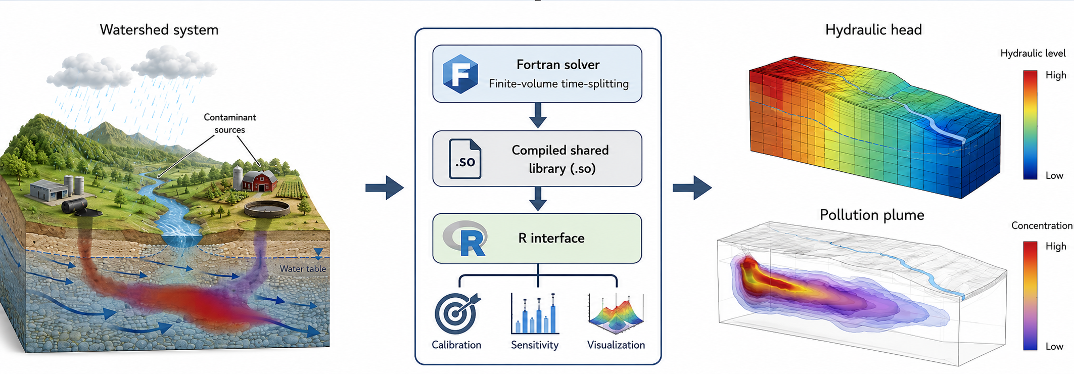
In the present study, Fortran is integrated with R to provide a practical and efficient tool for three-dimensional simulation of groundwater flow and contaminant transport through porous media, with relevance to watershed-scale applications. Beyond the integration of Fortran with R itself, the novelty of this study lies in the development of a reproducible and application-oriented framework for coupled three-dimensional groundwater flow and contaminant transport modeling, with enhanced capabilities for calibration, sensitivity analysis, and visualization within a unified workflow. The developed computational code was written in Fortran and interfaced with R to improve computational efficiency while enhancing flexibility for integrating external packages, calibration routines, and visualization tools. The Fortran-based code performs a three-dimensional simulation of groundwater flow and contaminant transport using a finite-volume time-splitting method, whereas R is used for data analysis, calibration, reproducibility, and visualization. The developed framework is intended to support the investigation of contaminant transport in heterogeneous media and to explore the interaction of multiple pollution sources within watershed systems.
2. Methodology
In the present study, an integrated framework combining Fortran and R is proposed. The following sections briefly describe these programming languages and their integration.
2.1. Fortran
Fortran is a programming language designed for high-performance computing and is widely used to solve complex scientific and engineering problems [31]. Although Fortran has undergone major revisions in recent decades, it still has limitations in visualization capabilities and interoperability with modern analytical tools. To address these limitations, external software packages such as MATFOR and Tecplot are commonly used for post-processing and visualization; however, reliance on separate programs can increase workflow complexity, processing time, and computational inefficiency.
2.2. The R Project
R is an open-source programming environment that has become increasingly popular for statistical computing, mathematical analysis, and graphical visualization. A large number of user-developed packages for statistics, computation, data analysis, and visualization can be readily installed and implemented in R. These packages make R highly flexible for processing data, performing numerical analysis, and presenting results. In addition, R is a powerful platform that can easily interface with other programming languages, including Fortran. This capability makes R useful for combining advanced analysis and visualization with efficient numerical computation.
2.3. Integration of R and Fortran
Interoperability between R and Fortran can be achieved by calling Fortran code compiled as dynamic-link libraries (DLLs) from within R. This DLL-based approach is practical and has long been used by software developers to efficiently distribute compiled code. The R environment further provides a convenient platform for integrating Fortran programs with a broad and continuously expanding set of statistical, numerical, and visualization packages.
3. Development of Fortran Code
To develop a numerical model for simulating groundwater flow and contaminant transport, a Fortran code was implemented to solve the governing equations of groundwater flow and solute transport. These equations are described in the following sections.
3.1. Groundwater Flow
Groundwater flow in the saturated zone is governed by a partial differential equation commonly referred to as the Boussinesq equation [36]:
|
```latex\frac{\partial }{\partial x}\left({k}_{xx}\frac{\partial h}{\partial x}\right)+\frac{\partial }{\partial y}\left({k}_{yy}\frac{\partial h}{\partial y}\right)+\frac{\partial }{\partial z}\left({k}_{zz}\frac{\partial h}{\partial z}\right)=S\frac{\partial h}{\partial t}``` |
(1) |
where the parameters are defined as follows: $${k}_{xx},{k}_{yy},{k}_{zz}$$: hydraulic conductivity in the $$x$$, $$y$$, and $$z$$ directions, respectively $$\left(L{T}^{-1}\right)$$; $$S$$: specific storage coefficient $$\left({L}^{-1}\right)$$.
3.2. Contaminant Transport
The transport of dissolved contaminants in groundwater is governed by the Advection–Dispersion–Reaction (ADR) equation [36]:
|
```latex\frac{\partial }{\partial x}\left({D}_{xx}\frac{\partial C}{\partial x}+{D}_{xy}\frac{\partial C}{\partial y}+{D}_{xz}\frac{\partial C}{\partial z}\right)+\frac{\partial }{\partial y}\left({D}_{yx}\frac{\partial C}{\partial x}+{D}_{yy}\frac{\partial C}{\partial y}+{D}_{yz}\frac{\partial C}{\partial z}\right)+\\\frac{\partial }{\partial z}\left({D}_{zx}\frac{\partial C}{\partial x}+{D}_{zy}\frac{\partial C}{\partial y}+{D}_{zz}\frac{\partial C}{\partial z}\right)-\frac{\partial \left({v}_{ax}C\right)}{\partial x}-\frac{\partial \left({v}_{ay}C\right)}{\partial y}-\frac{\partial \left({v}_{az}C\right)}{\partial z}-\lambda {R}_{d}C={R}_{d}\frac{\partial C}{\partial t}``` |
(2) |
where $$C$$ is the contaminant concentration $$\left(M{L}^{-3}\right)$$, $${D}_{ij}$$ are the dispersion coefficients in the three principal directions $$\left({L}^{2}{T}^{-1}\right)$$, and $${v}_{ai}$$ are the seepage velocities in the principal directions $$\left(L{T}^{-1}\right)$$. In addition, $$\lambda$$ is the contaminant decay rate, and $${R}_{d}$$ is the retardation factor used to account for the physical, biological, and chemical processes affecting contaminant transport through porous media.
3.3. Numerical Scheme
The developed Fortran code applies a finite-volume time-splitting method to solve the groundwater flow and contaminant transport equations. This method ensures mass conservation throughout the computational domain. Using the finite volume method, the groundwater flow flux for each control volume can be expressed as:
|
```latex{Flux}_{{flow}_{i+\frac{1}{2}}}={\varphi }_{i}-\frac{{K}_{ii}}{S}\left(\frac{\partial h}{\partial {x}_{i}}\right)=-\frac{{{\varphi }_{i}K}_{ii}}{S}\left(\frac{{h}_{i+1}^{2}-{h}_{i}^{1}}{\mathrm{\Delta }{x}_{i}}\right)``` |
(3) |
where $$Flu{x}_{flow}$$ represents the groundwater flow flux across a given portion of the boundary surface. $${\varphi }_{i}$$ is wetness index is the ratio of water height to total cell height.
Similarly, using the finite volume formulation, the flux terms for the advection and dispersion steps can be written as:
|
```latex{Flux}_{adv}=\frac{1}{{R}_{d}\mathrm{\Delta }\mathrm{t} }{\int }_{{t}^{n}}^{{t}^{n}+\frac{1}{2}}{v}_{{x}_{i}}Cdt``` |
(4) |
|
```latex{Flux}_{dis}=-\frac{1}{{R}_{d}\mathrm{\Delta }\mathrm{t} }{\int }_{{t}^{n}}^{{t}^{n}+\frac{1}{2}}{D}_{{x}_{i}}\frac{\partial C}{\partial {x}_{i}}dt``` |
(5) |
|
```latex{D}_{ii}=\frac{{\alpha }_{L}{v}_{i}^{2}}{\mid V\mid }+\frac{{\alpha }_{TH}{v}_{i}^{2}}{\mid V\mid }+\frac{{\alpha }_{TV}{v}_{i}^{2}}{\mid V\mid }+{D}^{*}``` |
(6) |
|
```latex\mid V\mid =\sqrt{{v}_{i}^{2}+{v}_{j}^{2}+{v}_{k}^{2}}``` |
(7) |
where, $${\alpha }_{L}$$, $${\alpha }_{TH},$$and $${\alpha }_{TV}$$ are longitudinal dispersivity, horizontal transverse dispersivity, and vertical transverse dispersivity, respectively. $${D}^{*}$$ is molecular diffusion.
In porous media, the longitudinal dispersivity along the direction of flow can be estimated using [36]:
|
```latex{\alpha }_{L}=0.2\text{\hspace{0.17em}}{L}^{0.44}``` |
(8) |
where $$L\left[L\right]$$ denotes the flow path length. The transverse dispersivity is typically lower than the longitudinal dispersivity and is commonly taken to be about one-hundredth of its value [36].
The governing equations are discretized in time using an implicit time-splitting scheme, while spatial discretization is performed using a finite-volume formulation that ensures mass conservation. For groundwater flow, upstream boundary conditions are implemented as specified-head (Dirichlet) or specified-flux (Neumann) conditions, depending on the physical configuration. At the downstream boundary, a free-surface seepage condition is applied, meaning that seepage is allowed only when the hydraulic head exceeds the boundary elevation; otherwise, no outflow is permitted. To represent drying and rewetting conditions, computational cells are classified as wet, partially wet, or dry. In fully wet cells, the flux is transferred through the entire cell, whereas in partially wet cells the flux is adjusted using a wetness index. The wetness index is defined as the ratio of water height to total cell height and is used to scale the flux accordingly. Dry cells are assigned zero mobile flux. For contaminant transport, the advection–dispersion equation is discretized using an implicit time-splitting scheme and solved based on the computed flow field. The dispersion tensor is formulated using the longitudinal and transverse dispersivities. Numerical stability is maintained through the appropriate selection of the time step in relation to the seepage velocity and dispersion coefficients.
More details regarding the numerical scheme used to solve the groundwater flow and contaminant transport equations can be found in [24,37].
4. Integration of Fortran with R
The process of linking Fortran code with R consists of four main steps:
-
Prepare and compile the Fortran subroutine
-
Compile the program to generate a shared library
-
Load the shared library in R
-
Run the R script to call the subroutine
Each of these steps is described in the following sections.
4.1. Preparation of the Fortran Subroutine
To interface Fortran code with R, the Fortran program must first be prepared as a subroutine rather than a function. For this purpose, the Fortran code developed for groundwater flow and contaminant transport was organized as a general subroutine that couples the simulation of groundwater flow and contaminant transport through porous media.
It should be noted that the variable types declared within the Fortran subroutine must be consistent with the corresponding variable types defined in R.
The main subroutine includes four internal subroutines that handle geometry input, definition of the initial and boundary conditions for groundwater flow, definition of the initial and boundary conditions for contaminant transport, and solution of the coupled groundwater flow and contaminant transport system. The fortran subroutine for groundwater flow contaminant transport is listed in Box 1.
Box 1. Fortran Subroutine for Groundwater Flow Contaminant Transport.
! THIS SUBROUTINE SOLVES THE 3D GROUNDWATER FLOW & CONTAMINANT TRANSPORT
SUBROUTINE FLTR (NRO, NCO, NTC, IB, IE, JBEI, KBEI, IBB, IEB, JB, JE, IBEJ, KBEJ, JBB, JEB, KB, KE, IBEK, JBEK, KBB, KEB, DELTAX, DELTAY, DELTAZ, dt, nt, NRO, NCO, NTC, IB, IE, JBEI, KBEI, IBB, IEB, JB, JE, IBEJ, KBEJ, JBB, JEB, KB, KE, IBEK, JBEK, KBB, KEB, B, BCP, BCT, KX, KY, KZ, SS, H3D, C3D, X, Y, Z, TEL, Dm, ALFAL, ALFATV, ALFATH, GAMA, Rd, POR, D3D, TETA)
IMPLICIT NONE
INTEGER, PARAMETER: mx = 100
DOUBLE PRECISION H3D (mx, mx, mx), C3D (mx, mx, mx), BCP (mx), BCT (mx), X (mx, mx, mx), Y (mx, mx, mx), Z (mx, mx, mx), DELTAX (mx, mx, mx), DELTAY (mx, mx, mx), DELTAZ (mx, mx, mx)
DOUBLE PRECISION dt, TEL, WELLC1, WELLC2, Dm, ALFAL, ALFATV, ALFATH, GAMA, DENS, Kd, Rd, SS, POR, D3D, KX, KY, KZ, TETA
INTEGER IB (mx, mx), IE (mx, mx), JBEI (mx, mx), KBEI (mx, mx), IBB (mx, mx), IEB (mx, mx), JB (mx, mx), JE (mx, mx), IBEJ (mx, mx), KBEJ (mx, mx), JBB (mx, mx), JEB (mx, mx), KB (mx, mx), KE (mx, mx), IBEK (mx, mx), JBEK (mx, mx), KBB (mx, mx), KEB (mx, mx), B (mx)
INTEGER nt, NRO, NCO, NTC
! MAIN SUBROUTINES
CALL GEO (NRO, NCO, NTC, IB, IE, JBEI, KBEI, IBB, IEB, JB, JE, IBEJ, KBEJ, JBB, JEB, KB, KE, IBEK, JBEK, KBB, KEB)
CALL PHTRDATA (DELTAX, DELTAY, DELTAZ, dt, nt, B, BCP, BCT, KX, KY, KZ, SS, NRO, NCO, NTC, X, Y, Z, TEL, Dm, ALFAL, ALFATV, ALFATH, GAMA, Rd, POR, D3D, TETA)
CALL ICPHL (NRO, NCO, NTC, H3D, C3D, X, Y, Z)
CALL PHTR (DELTAX, DELTAY, DELTAZ, dt, nt, NRO, NCO, NTC, IB, IE, JBEI, KBEI, IBB, IEB, JB, JE, IBEJ, KBEJ, JBB, JEB, KB, KE, IBEK, JBEK, KBB, KEB, B, BCP, BCT, KX, KY, KZ, SS, H3D, C3D, X, Y, Z, TEL, Dm, ALFAL, ALFATV, ALFATH, GAMA, Rd, POR, D3D, TETA)
RETURN
END SUBROUTINE
4.2. Compile and Load the Shared Library in R
Once the Fortran code has been prepared in the required format, it must be compiled into a shared object file before being executed within R, thereby allowing dynamic linking at runtime. In the present study, the Fortran code was compiled into a shared object file (.so), which enables direct linking and execution from the R environment. The compile and load fortran library in R is listed in Box 2.
Box 2. Compile and Load Fortran Library in R.
# INTEL FORTRAN COMPILER
ifort -fpic -shared FLTR.f90 -o FLTR.so
dyn.load("FLTR.so")
Before the Fortran subroutines can be utilized in R, the compiled shared library must first be loaded. In this study, the dyn.load command is used to load the Fortran code into the R environment. This command allows shared object files, also referred to as dynamically loadable libraries (DLLs), to be loaded and unloaded as needed.
4.3. Run the R Program to Call the Subroutine
In the final step, the Fortran subroutine is called directly from within R using the .Fortran() function, which is specifically designed to invoke Fortran subroutines. When using this function, the name of the Fortran subroutine must be specified, and the input arguments must be provided in a format consistent with the corresponding Fortran data types. The call fortran subroutine from R is listed in Box 3.
Box 3. Call Fortran Subroutine from R.
Result <- .Fortran ("FLTR", NRO, NCO, NTC, IB, IE, JBEI, KBEI, IBB, IEB, JB, JE, IBEJ, KBEJ, JBB, JEB, KB, KE, IBEK, JBEK, KBB, KEB, DELTAX, DELTAY, DELTAZ, dt, nt, NRO, NCO, NTC, IB, IE, JBEI, KBEI, IBB, IEB, JB, JE, IBEJ, KBEJ, JBB, JEB, KB, KE, IBEK, JBEK, KBB, KEB, B, BCP, BCT, KX, KY, KZ, SS, H3D, C3D, X, Y, Z, TEL, Dm, ALFAL, ALFATV, ALFATH, GAMA, Rd, POR, D3D, TETA)
For clarity, the input variables are grouped into categories representing grid configuration, hydraulic properties, boundary conditions, and transport parameters. The input and output parameters used in the Fortran subroutine are summarized in Table 1.
Table 1. Description of input arguments used in the Fortran subroutine.
|
Variable |
Description |
Unit |
|---|---|---|
|
NRO, NCO, NTC |
Number of grid cells in x, y, z directions |
– |
|
KX, KY, KZ |
Hydraulic conductivity in x, y, z directions |
m/s |
|
SS |
Specific storage coefficient |
1/m |
|
POR |
Porosity of the medium |
– |
|
H3D |
Hydraulic head distribution |
m |
|
C3D |
Contaminant concentration |
mg/L |
|
DELTAX, DELTAY, DELTAZ |
Grid spacing |
m |
|
dt |
Time step |
s |
|
nt |
Number of time steps |
– |
|
Dm |
Molecular diffusion coefficient |
m2/s |
|
ALFAL, ALFATV, ALFATH |
Dispersivity coefficients |
m |
5. Validation
In this section, two test cases are presented to evaluate the performance of the integrated model. The first test case is used to verify the groundwater flow simulation, while the second test case assesses the model’s capability to simulate contaminant transport.
5.1. Validation of Groundwater Flow Model
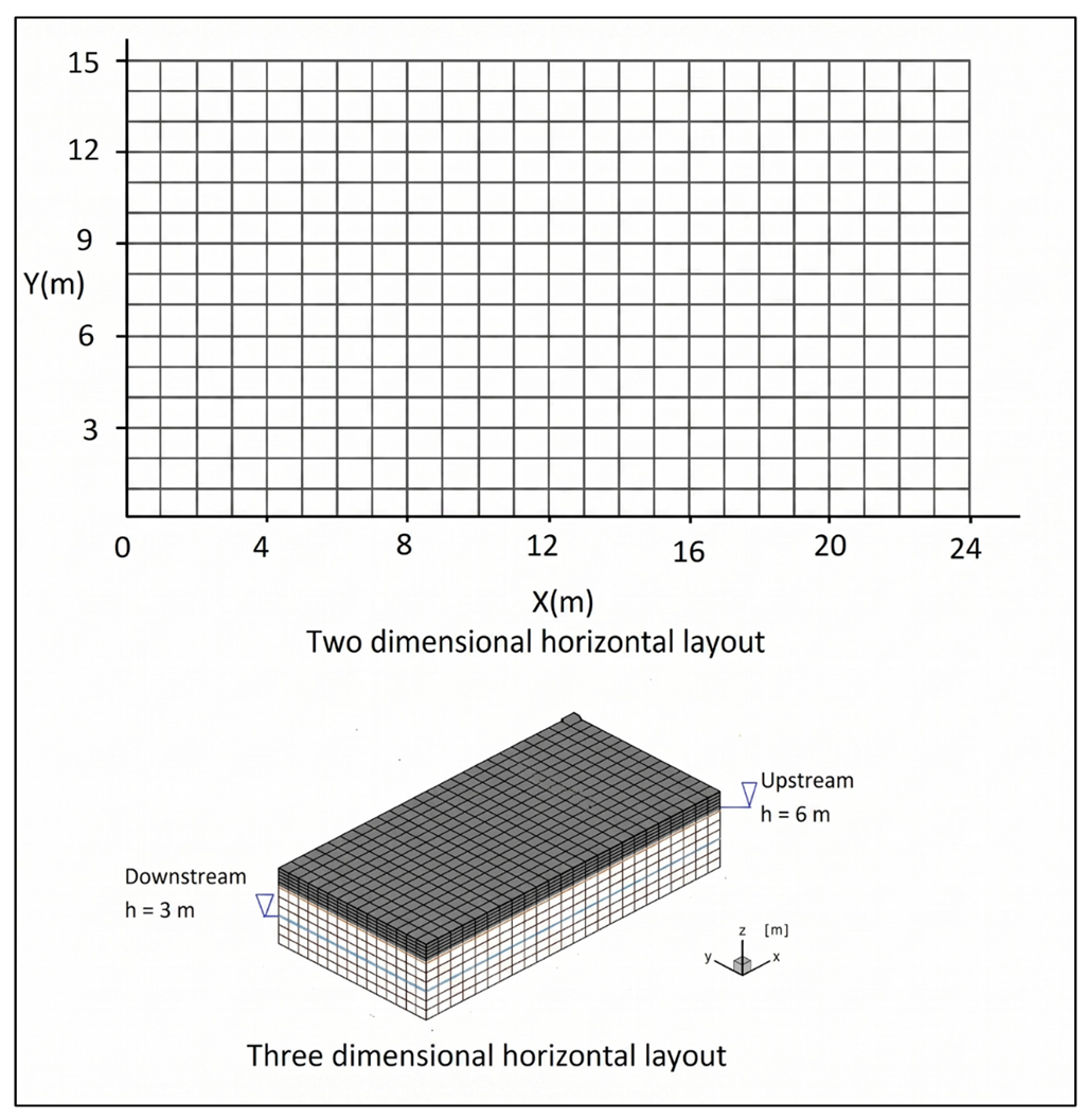
The performance of the integrated model for the simulation of groundwater flow and free surface seepages, assessed by the first test case, and the results of the integrated model are compared with the analytical solution. The sketch layout of the first test case with dimensions of 24 m × 15 m × 7 m is depicted in Figure 1. As shown, constant head boundary conditions are applied at the upstream and downstream boundaries. The upstream and downstream boundary conditions are 6 m and 3 m, respectively. The hydraulic conductivity of the homogeneous porous media is considered as 2 × 10⁻⁵ m/s.
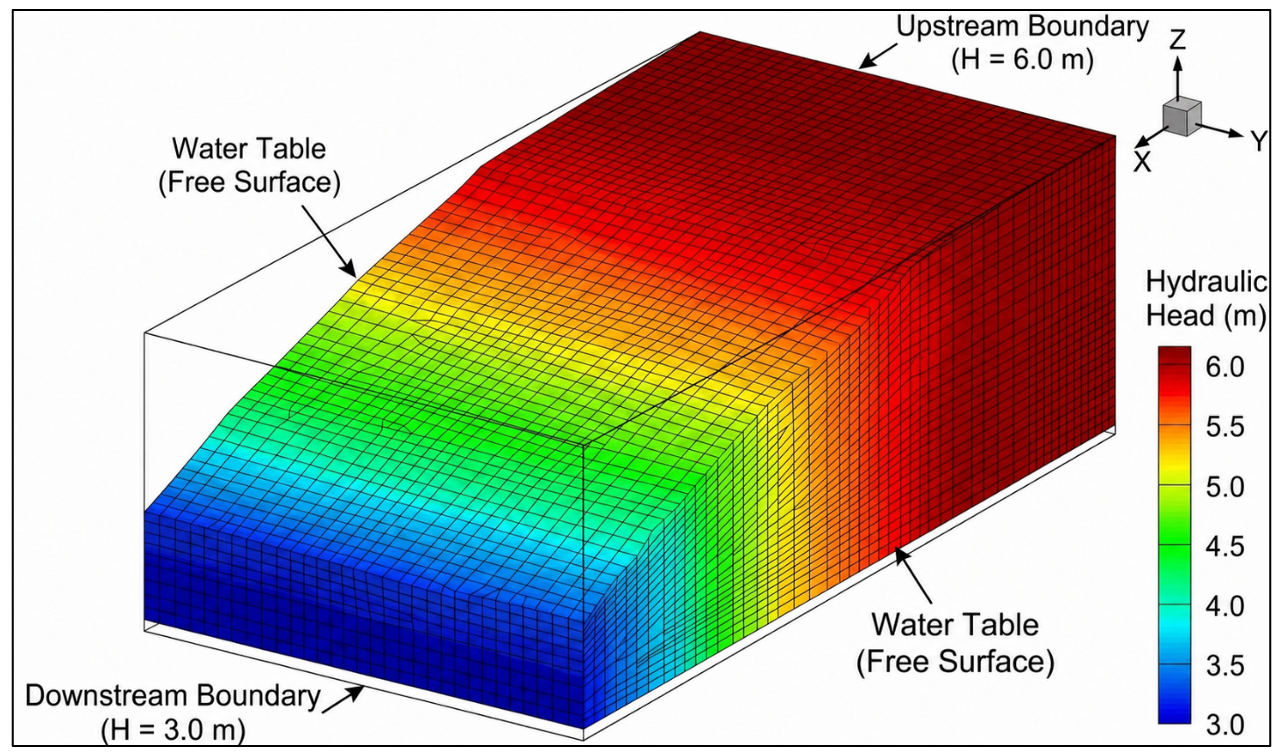
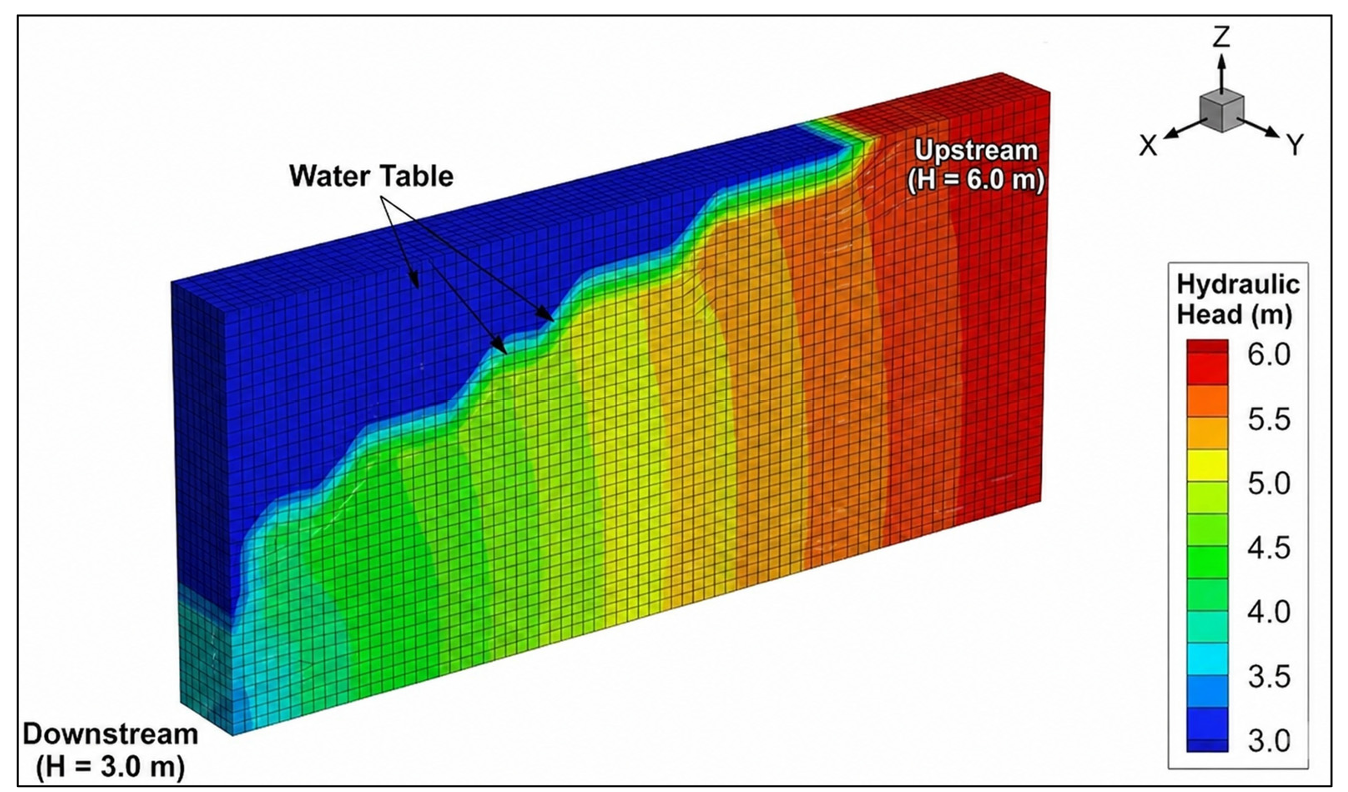
Figure 2 presents the phreatic surface predicted by the numerical model in both two-dimensional (2D) and three-dimensional (3D) representations. As shown, the groundwater hydraulic head decreases gradually from upstream to downstream within the homogeneous porous medium. This progressive reduction in hydraulic head results in an approximately constant hydraulic gradient and a uniform velocity field throughout the domain.
 (a) |
 |
|
(b) |
Figure 2. Numerical results of groundwater flow. (a) Three-dimensional view; (b) two-dimensional view.
To validate the integrated numerical model, its results were compared with the analytical solution. The analytical solution for predicting the water table in porous media was adopted from [38]. Figure 3 compares the integrated numerical model results with the analytical solution. The comparison plot was produced in the R environment, and several statistical indices were also calculated to assess model performance.
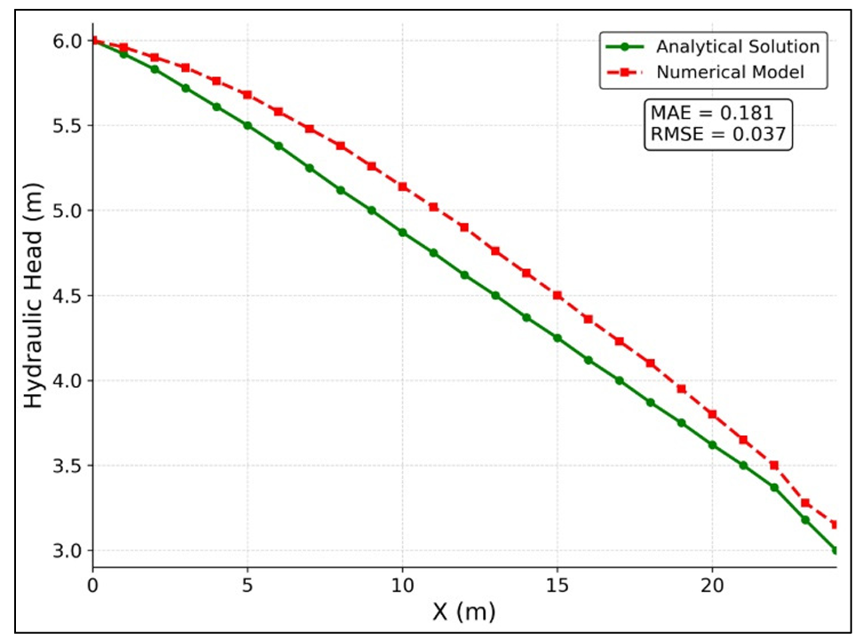
Figure 3 shows good agreement between the numerical and analytical solutions, with mean absolute error (MAE) and root mean square error (RMSE) values of 0.181 and 0.037, respectively. These results confirm the satisfactory performance of the groundwater flow model.
5.2. Validation of Contaminant Transport Model
To assess the validity and reliability of the integrated model for contaminant transport simulation, a second test case was considered. The contaminant transport results generated by the developed model were compared with an analytical solution. The analytical solution for predicting the pollutant transport through saturated porous media was adopted from [39]. In this test case, the porous medium had a length of 100 m (𝐿 = 100 m), and the velocity field consisted only of a horizontal velocity component ($${V}_{x}$$) of 0.005 m/s. A point-source contaminant with a constant concentration of 100 mg/L ($${C}_{0}=100$$) was injected into the porous medium at location (10, 50, 50) in the Cartesian coordinate system. The dispersion coefficient was assumed to be 10−7 m2/s, and the retardation factor was set to 1.0.
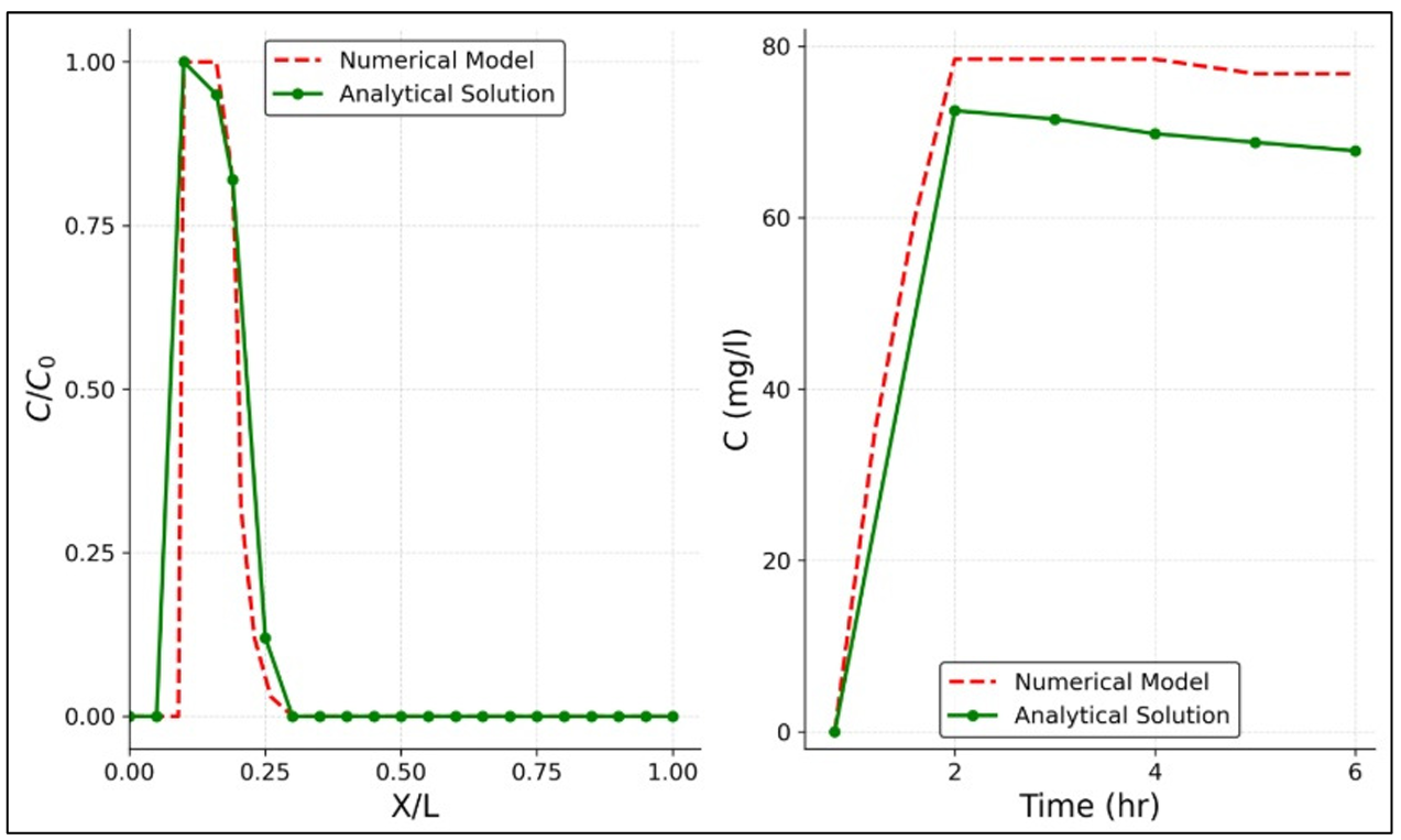
The analytical and numerical solutions for contaminant transport were compared using an R script. Figure 4 compares the numerical and analytical solutions for solute transport, showing (a) the concentration profile after 1 h at y = 30 m, and (b) the temporal variation of contaminant concentration at the coordinate (40, 50, 50).
Figure 4 shows good agreement between the numerical results and the analytical approximation, indicating that the contaminant transport model can accurately predict the temporal and spatial distribution of contaminant concentrations in porous media.
Since the groundwater flow and contaminant transport components were verified separately through the test cases, the integrated model is demonstrated to be capable of simulating groundwater flow and contaminant transport through porous media.
 |
|
|
(a) |
(b) |
Figure 4. Comparison of numerical and analytical solutions of solute transport (a) after 1 h at y = 30 m, (b) pollution distribution at the (40, 50, 50) coordinate at different times.
6. Model Application
To demonstrate the practical applicability of the developed model, two illustrative examples are presented in this section. The first example examines the effect of porous-medium heterogeneity on groundwater flow and contaminant transport, while the second investigates the interaction among multiple pollution sources.
A three-dimensional porous medium with dimensions of 20 m × 10 m × 10 m is considered for this purpose. The upstream and downstream boundary heads are prescribed as 10 m and 1 m, respectively. The computational domain is shown in Figure 5. The developed Fortran model for groundwater flow and contaminant transport simulation requires several input parameters describing the porous medium, including hydraulic conductivity, effective porosity, and specific yield, as well as contaminant-related parameters such as the dispersion coefficient and the locations of pollution sources.
Since model inputs play a critical role in parameter estimation, particularly in regional- or watershed-scale applications, all input values were selected based on a review of the relevant literature on groundwater flow and contaminant transport modeling. The corresponding parameters are listed in Table 2.
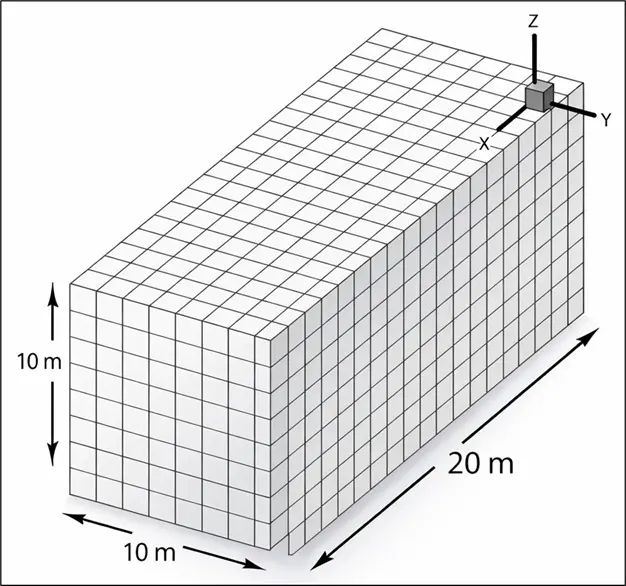
Table 2. Input parameter.
|
Parameter |
Value |
Unit |
|---|---|---|
|
Hydraulic Conductivity |
1 × 10⁻³ |
m/s |
|
Effective Porosity |
0.294 |
|
|
Molecular Dispersion Coefficient |
4 × 10⁻⁹ |
m2/s |
6.1. Effect of Heterogenous Layers
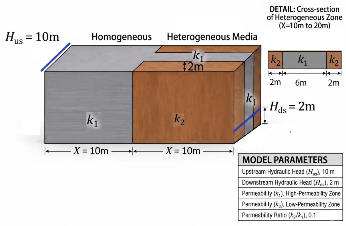
In this example, groundwater flow and contaminant plume evolution in homogeneous and heterogeneous porous media are compared. A heterogeneous zone composed of two layers with contrasting permeabilities is considered. The ratio of the hydraulic conductivity of the low-permeability layer to that of the high-permeability layer is 0.1 (𝑘2/𝑘1 = 0.1), and the effective porosity of the low-permeability zone is taken as 0.341.
Each low-permeability layer has a length of 10 m and a width of 2 m and is located along the right and left sides of the porous medium. The layers begin at the midpoint of the computational domain (x = 10 m) and extend toward the downstream boundary, as shown in Figure 6. In the implementation of R, the heterogeneous soil layers are defined as a vector. Two contaminant sources, each with a concentration of 10 mg/L, are introduced into the porous medium for 5 min at coordinates (1, 3, 2) and (1, 3, 5).
The effects of the low permeability layer on groundwater flow and contaminant transport are shown in Figure 7 and Figure 8.
 |
|
(a) |
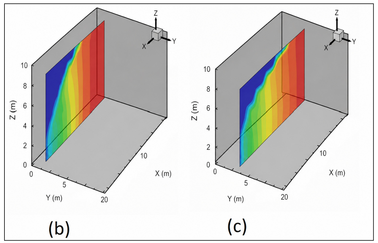 |
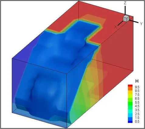
Figure 7. Groundwater flow. (a) Three-dimensional model; (b) heterogeneous zone; (c) homogeneous zone.
The groundwater flow simulation results indicate that the permeability distribution within the porous medium has a direct effect on seepage flow. In the homogeneous zone, the hydraulic gradient remains nearly constant, and the velocity field is approximately uniform. By contrast, the heterogeneous zone exhibits a pronounced change in hydraulic gradient.
Within the heterogeneous zone, the low-permeability layers act as semi-impermeable barriers that restrict groundwater flow and seepage. Flow velocities are higher in layers with greater hydraulic conductivity. Consequently, the low-permeability layers impede seepage, resulting in an increase in hydraulic head within the adjacent high-permeability layer and saturation of the upstream region.
As shown, the water-table slope across the low-permeability layer decreases markedly. The velocity field in the heterogeneous zone varies because the layers possess different hydraulic conductivities. Higher velocities occur in the high-permeability layer, whereas velocities decrease substantially within the low-permeability layer.
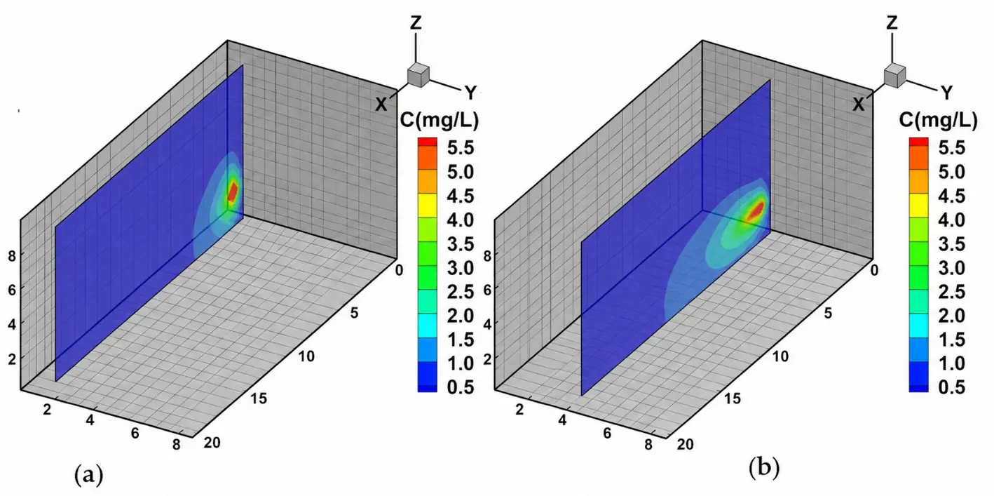
Figure 8 and Figure 9 further indicate that the contaminant plume in the homogeneous zone experiences faster advective transport than in the heterogeneous zone. Therefore, the contaminant arrival time in the homogeneous porous medium is shorter than in the medium containing low-permeability layers.
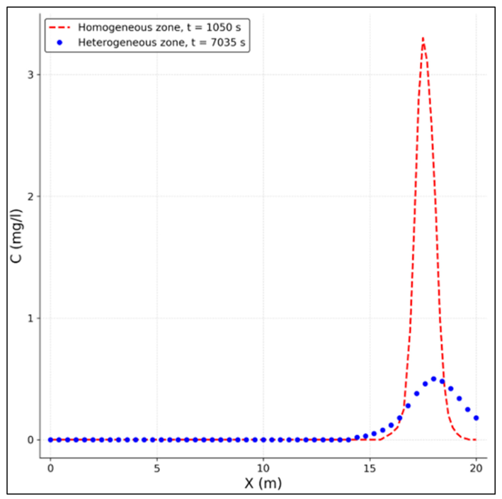
The heterogeneous case consists of two low-permeability zones located on the left and right sides of the model, each occupying approximately half of the domain length, while the central part remains more permeable. Compared with the homogeneous case, the heterogeneous configuration significantly affects contaminant transport. The arrival time increases from 1050 to 7035, representing about a 570% increase, or approximately 6.7 times. In addition, the contaminant mass passing the downstream control plane decreases from 3.3 to 1.5, corresponding to a reduction of about 54.5%. These results demonstrate that the presence of low-permeability zones delays plume migration and reduces the mass of contaminants reaching the downstream boundary.
The contaminant transport results also demonstrate that the low-permeability layers significantly reduce the velocity field in the heterogeneous zone, thereby decreasing the advective transport rate of the solute.
6.2. Effect of Multi-Point Sources of Pollution
To evaluate the effect of multiple pollution sources on groundwater flow and contaminant transport, two-point sources were considered. The Cartesian coordinates of the sources were C1 = (5, 7, 3) and C2 = (3, 3, 4).
Each source was assigned a constant concentration of 10 mg/L and introduced into the homogeneous porous medium for a duration of two minutes. The contaminant plumes produced by these multiple sources are presented in Figure 10, Figure 11 and Figure 12.
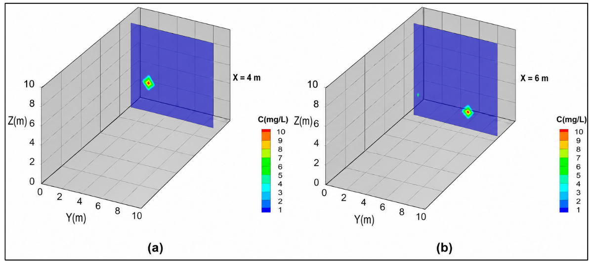
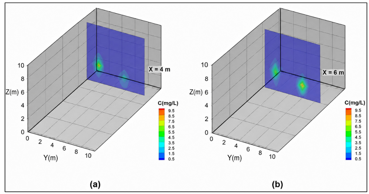
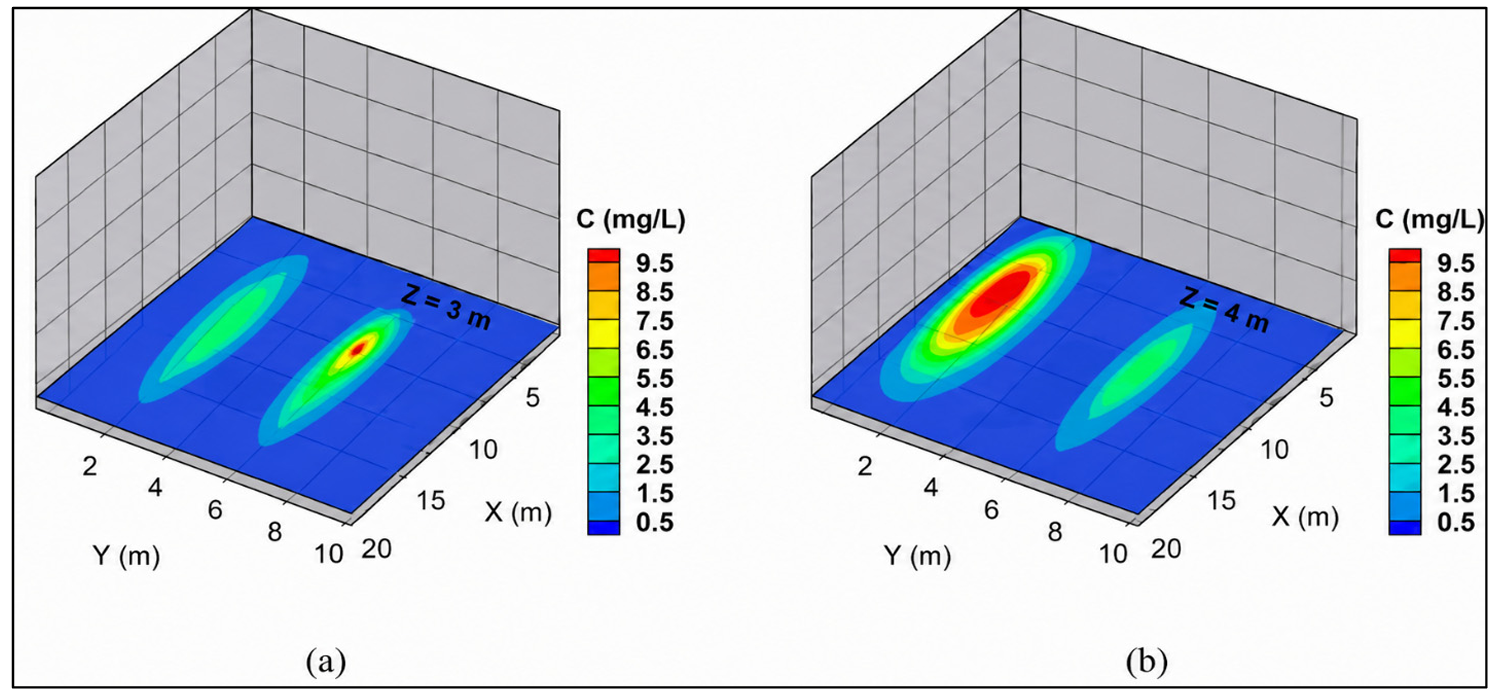
Figure 10, Figure 11, Figure 12 and Figure 13 show that the pollutant plumes do not exhibit significant interaction in any direction; therefore, the migration behavior of each point source can be evaluated independently. Since advection is the dominant transport mechanism in this example, contaminant migration is governed primarily by advective transport. In addition, the small dispersion coefficients result in limited plume spreading. These results demonstrate that plume interaction depends strongly on the magnitude of dispersion. With increasing dispersion, the plumes associated with the point sources interact more significantly.
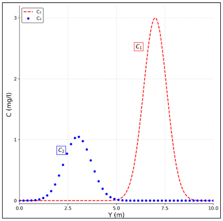
It should be noted that plume interaction is strongly dependent on source spacing, dispersivity, flow velocity, and other porous media parameters; therefore, the observed limited interaction in this study is specific to the selected conditions and should not be generalized.
7. Conclusions
Many numerical models and computational codes in hydrology and hydraulics have traditionally been developed in Fortran. Although Fortran offers many advantages, particularly for high-performance scientific computing, some limitations remain, especially in output visualization and interoperability with modern analytical tools. To address these limitations, this study presented an approach for integrating R and Fortran by loading and calling Fortran source code compiled as dynamic libraries within the R environment. The proposed framework provides an integrated numerical platform for efficient data preparation, calibration, analysis, and visualization. In this work, a three-dimensional Fortran code for groundwater flow and solute transport was executed through R. The integrated framework demonstrated the ability to simulate groundwater flow and contaminant transport through porous media while supporting reproducible data processing, calibration, and visualization. This integrated, and reproducible framework is particularly relevant to watershed applications, where groundwater flow and contaminant transport influence stream–aquifer interactions, baseflow dynamics, and overall watershed water quality. Favorable agreement between the numerical results and analytical solutions confirmed the satisfactory performance of the developed model. In addition, the framework can interface with modern software environments and leverage a wide range of R packages, including those for uncertainty analysis, inverse modeling, and statistical graphics, to enhance the simulation of groundwater flow and contaminant transport. Application of the model to heterogeneous porous media further showed that low-permeability layers strongly influence the arrival time of pollutants and play a major role in controlling interactions among multiple point pollution sources. Moreover, the results demonstrated that the dispersion rate significantly affects plume interaction.
Ethics Statement
Not applicable.
Informed Consent Statement
Not applicable.
Data Availability Statement
To support reproducibility and transparency, the Fortran and R source codes developed in this study are publicly available at the following GitHub repository: https://github.com/Ahmadi-Hosein, accessed on 25 April 2026.
Funding
This research received no external funding.
Declaration of Competing Interest
The author declares that he has no known competing financial interests or personal relationships that could have appeared to influence the work reported in this paper.
References
- Hanoon MS, Ahmed AN, Fai CM, Birima AH, Razzaq A, Sherif M, et al. Application of artificial intelligence models for modeling water quality in groundwater: Comprehensive review, evaluation and future trends. Water Air Soil Pollut. 2021, 232, 411. DOI:10.1007/s11270-021-05311-z [Google Scholar]
- International Association of Hydrogeologists. Groundwater—More About the Hidden Resource; International Association of Hydrogeologists: Goring, UK, 2020. [Google Scholar]
- Ramos-Ruiz A, Wilkening JV, Field JA, Sierra-Alvarez R. Leaching of cadmium and tellurium from cadmium telluride (CdTe) thin-film solar panels under simulated landfill conditions. J. Hazard. Mater. 2017, 336, 57–64. DOI:10.1016/j.jhazmat.2017.04.052 [Google Scholar]
- Park S, Sung K. Leaching potential of multi-metal-contaminated soil in chelate-aided remediation. Water Air Soil Pollut. 2020, 231, 40. DOI:10.1007/s11270-020-4412-6 [Google Scholar]
- Fairchild DM. A national assessment of ground water contamination from pesticides and fertilizers. In Ground Water Quality and Agricultural Practices; CRC Press: Boca Raton, FL, USA, 2020; pp. 273–294. [Google Scholar]
- Uliana MM. Identifying the source of saline groundwater contamination using geochemical data and modeling. Environ. Eng. Geosci. 2005, 11, 107–123. DOI:10.2113/11.2.107 [Google Scholar]
- Shang F, Ren S, Yang P, Li C, Xue Y, Huang L. Modeling the risk of the salt for polluting groundwater irrigation with recycled water and ground water using HYDRUS-1 D. Water Air Soil Pollut. 2016, 227, 189. DOI:10.1007/s11270-016-2875-2 [Google Scholar]
- Kuriqi A, Abd-Elaty I. Groundwater salinization risk in coastal regions triggered by earthquake-induced saltwater intrusion. Stoch. Environ. Res. Risk Assess. 2024, 38, 3093–3108. DOI:10.1007/s00477-024-02734-y [Google Scholar]
- Ite AE, Harry TA, Obadimu CO, Asuaiko ER, Inim IJ. Petroleum hydrocarbons contamination of surface water and groundwater in the Niger Delta region of Nigeria. J. Environ. Pollut. Hum. Health 2018, 6, 51–61. DOI:10.12691/jephh-6-2-2 [Google Scholar]
- Yoon S, Yeom K, Kim Y, Park B, Park J, Kim H, et al. Management of naturally occurring asbestos area in Republic of Korea. Environ. Eng. Geosci. 2020, 26, 79–87. DOI:10.2113/EEG-2287 [Google Scholar]
- Singh A. Decision support for on-farm water management and long-term agricultural sustainability in a semi-arid region of India. J. Hydrol. 2010, 391, 63–76. DOI:10.1016/j.jhydrol.2010.07.006 [Google Scholar]
- Ahmadi H, Kilanehei F, Nazari-Sharabian M. Impact of Pumping Rate on Contaminant Transport in Groundwater—A Numerical Study. Hydrology 2021, 8, 103. DOI:10.3390/hydrology8030103 [Google Scholar]
- Conant B, Jr., Robinson CE, Hinton MJ, Russell HA. A framework for conceptualizing groundwater-surface water interactions and identifying potential impacts on water quality, water quantity, and ecosystems. J. Hydrol. 2019, 574, 609–627. DOI:10.1016/j.jhydrol.2019.04.050 [Google Scholar]
- Ahmadi H. Modeling of groundwater-surface water interactions: A review of integration strategies. ISH J. Hydraul. Eng. 2024, 30, 132–146. DOI:10.1080/09715010.2023.2263434 [Google Scholar]
- El Himer H, Fakir Y, Stigter TY, Lepage M, El Mandour A, Ribeiro L. Assessment of groundwater vulnerability to pollution of a wetland watershed: The case study of the Oualidia-Sidi Moussa wetland, Morocco. Aquat. Ecosyst. Health Manag. 2013, 16, 205–215. DOI:10.1080/14634988.2013.788427 [Google Scholar]
- Ahmadi H. An overview of non-point source pollution modeling: Current status and future prospect. J. Civ. Eng. Res. Technol. 2023, 5, 1–8. DOI:10.47363/JCERT/2023(5)140 [Google Scholar]
- Du J, Jia C, Ding Y, Yang X, Feng K, Wei M. Advancing wetland groundwater pollution zoning: A novel integration of Monte Carlo health risk modeling and machine learning. J. Hazard. Mater. 2025, 494, 138412. DOI:10.1016/j.jhazmat.2025.138412 [Google Scholar]
- Ahmadi H. An implicit numerical model for solving free-surface seepage problems. ISH J. Hydraul. Eng. 2022, 28, 391–399. DOI:10.1080/09715010.2021.1925982 [Google Scholar]
- Ahmadi H. A numerical scheme for advection dominated problems based on a Lagrange interpolation. Groundw. Sustain. Dev. 2021, 13, 100542. DOI:10.1016/j.gsd.2020.100542 [Google Scholar]
- Malaguerra F, Albrechtsen HJ, Binning PJ. Assessment of the contamination of drinking water supply wells by pesticides from surface water resources using a finite element reactive transport model and global sensitivity analysis techniques. J. Hydrol. 2013, 476, 321–331. DOI:10.1016/j.jhydrol.2012.11.010 [Google Scholar]
- Zhou Z, Cui Z, Xu S. Impact of soil heterogeneity and NAPL presence on stable carbon isotope signature distribution during reactive transport. Water Air Soil Pollut. 2017, 228, 408. DOI:10.1007/s11270-017-3528-9 [Google Scholar]
- Xie Y, Wu J, Nan T, Xue Y, Xie C, Ji H. Efficient triple-grid multiscale finite element method for 3D groundwater flow simulation in heterogeneous porous media. J. Hydrol. 2017, 546, 503–514. DOI:10.1016/j.jhydrol.2017.01.027 [Google Scholar]
- Ramasomanana F, Fahs M, Baalousha HM, Barth N, Ahzi S. An efficient ellam implementation for modeling solute transport in fractured porous media. Water Air Soil Pollut. 2018, 229, 46. DOI:10.1007/s11270-018-3690-8 [Google Scholar]
- Ahmadi H, Namin MM, Kilanehei F. Development a numerical model of flow and contaminant transport in layered soils. Adv. Environ. Res. 2016, 5, 263–282. DOI:10.12989/aer.2016.5.4.263 [Google Scholar]
- Shokri N, Montazeri Namin M, Farhoudi J. An implicit 2D hydrodynamic numerical model for free surface–subsurface coupled flow problems. Int. J. Numer. Methods Fluids 2018, 87, 343–357. DOI:10.1002/fld.4494 [Google Scholar]
- Guneshwor L, Eldho TI, Kumar AV. Identification of groundwater contamination sources using meshfree RPCM simulation and particle swarm optimization. Water Resour. Manag. 2018, 32, 1517–1538. DOI:10.1007/s11269-017-1885-1 [Google Scholar]
- Rupali S, Sawant VA. 1 D contaminant transport through unsaturated stratified media using EFGM. Adv. Environ. Res. 2019, 8, 1–21. Available online: https://www.dbpia.co.kr/Journal/articleDetail?nodeId=NODE10234655 (accessed on 1 September 2019).
- Basser H, Rudman M, Daly E. Smoothed Particle Hydrodynamics modelling of fresh and saltwater dynamics in porous media. J. Hydrol. 2019, 576, 370–380. DOI:10.1016/j.jhydrol.2019.06.048 [Google Scholar]
- Diersch HJ, Kolditz O. Variable-density flow and transport in porous media: Approaches and challenges. Adv. Water Resour. 2002, 25, 899–944. DOI:10.1016/S0309-1708(02)00063-5 [Google Scholar]
- Fakoor M, Zadeh PM, Eskandari HM. Developing an optimal layout design of a satellite system by considering natural frequency and attitude control constraints. Aerosp. Sci. Technol. 2017, 71, 172–188. DOI:10.1016/j.ast.2017.09.012 [Google Scholar]
- Thyer M, Leonard M, Kavetski D, Need S, Renard B. The open source RFortran library for accessing R from Fortran, with applications in environmental modelling. Environ. Model. Softw. 2011, 26, 219–234. DOI:10.1016/j.envsoft.2010.05.007 [Google Scholar]
- Schlather M, Huwe B. The use of the language interface of R: Two examples for modelling water flux and solute transport. Comput. Geosci. 2004, 30, 197–201. DOI:10.1016/j.cageo.2003.08.007 [Google Scholar]
- Wu Y, Liu S. Automating calibration, sensitivity and uncertainty analysis of complex models using the R package Flexible Modeling Environment (FME): SWAT as an example. Environ. Model. Softw. 2012, 31, 99–109. DOI:10.1016/j.envsoft.2011.11.013 [Google Scholar]
- Coron L, Thirel G, Delaigue O, Perrin C, Andréassian V. The suite of lumped GR hydrological models in an R package. Environ. Model. Softw. 2017, 94, 166–171. DOI:10.1016/j.envsoft.2017.05.002 [Google Scholar]
- Eddelbuettel D, Balamuta JJ. Extending R with C++: A brief introduction to Rcpp. Am. Stat. 2018, 72, 28–36. DOI:10.1080/00031305.2017.1375990 [Google Scholar]
- Bear J. Hydraulics of Groundwater; McGraw-Hill: New York, NY, USA, 1979. [Google Scholar]
- Ahmadi H, Kilanehei F, Mostafazadeh F, Hassanlourad M. Numerical and Experimental Simulation of Contaminant Transport Through Porous Media with a Sublayer. Int. J. Civ. Eng. 2025, 23, 1183–1202. DOI:10.1007/s40999-025-01100-5 [Google Scholar]
- Xin Y, Zhou Z, Li M, Zhuang C. Analytical solutions for unsteady groundwater flow in an unconfined aquifer under complex boundary conditions. Water 2020, 12, 75. DOI:10.3390/w12010075 [Google Scholar]
- Tindall JA, Kunkel JR, Anderson DE. Unsaturated Zone Hydrology for Scientists and Engineers; Upper Rentice Hall: Saddle River, NJ, USA, 1999; Volume 4. [Google Scholar]