Integrating Copernicus Earth Observation and Artificial Intelligence for Habitat Suitability Modeling of Pinctada radiata in Semi-Enclosed Coastal Watersheds of Central Greece

Integrating Copernicus Earth Observation and Artificial Intelligence for Habitat Suitability Modeling of Pinctada radiata in Semi-Enclosed Coastal Watersheds of Central Greece
Received: 02 December 2025 Revised: 06 January 2026 Accepted: 09 March 2026 Published: 23 March 2026

© 2026 The authors. This is an open access article under the Creative Commons Attribution 4.0 International License (https://creativecommons.org/licenses/by/4.0/).
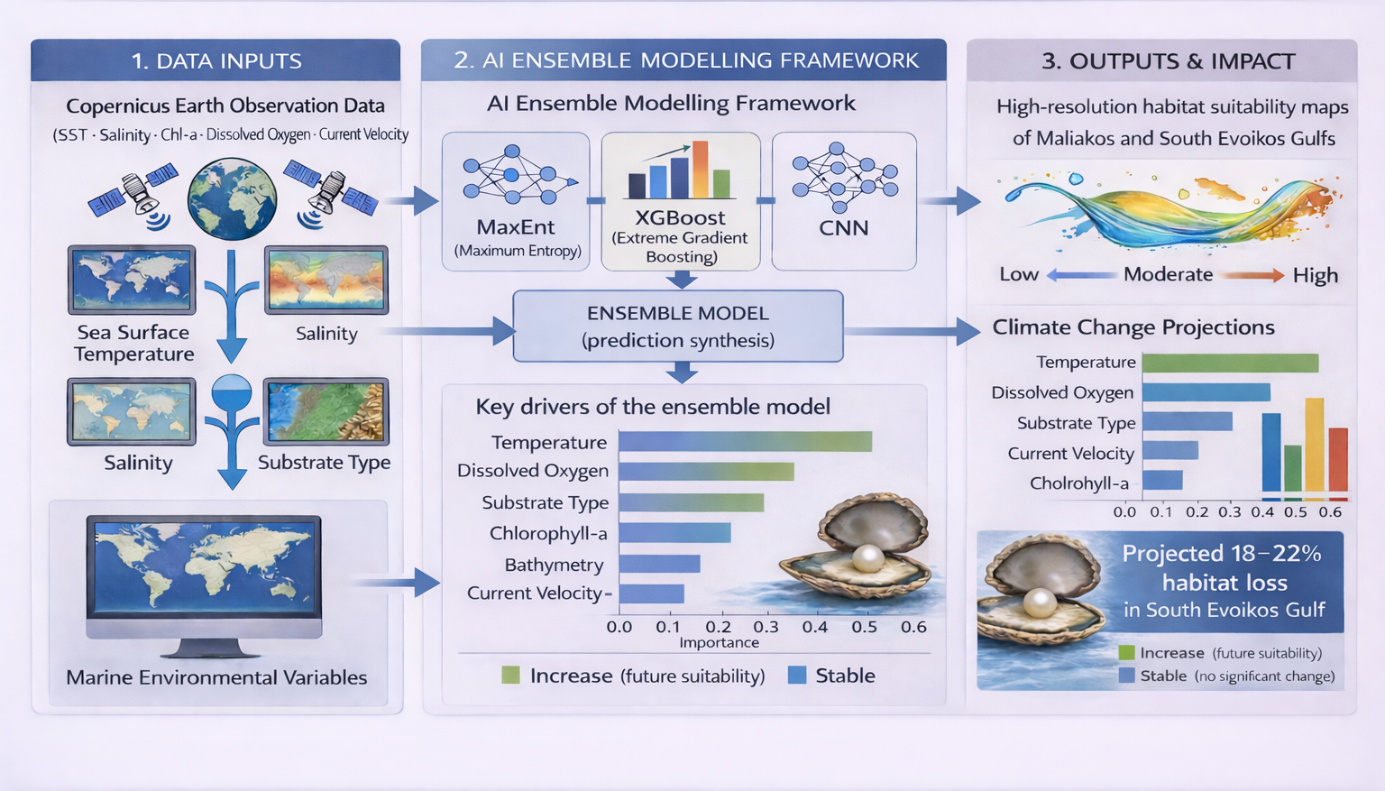
Graphical Abstract
1. Introduction
Semi-enclosed coastal systems are particularly sensitive to marine environments. Their restricted water exchange pronounced vertical stratification, and the interplay of physical and biogeochemical processes creates conditions that can strongly affect how marine communities are structured and function [1,2,3,4]. In the Mediterranean, these transitional areas support high biodiversity and important fisheries habitats, and they are often zones of elevated productivity. At the same time, they receive substantial inputs of nutrients and other land-derived pressures, which can intensify existing stressors [5,6,7]. Because these systems are only partly connected to the open sea, they tend to be especially vulnerable to warming, eutrophication, and, in many cases, seasonal or episodic hypoxia factors known to affect benthic communities and reduce ecosystem resilience [8,9,10,11]. As these pressures continue to escalate, understanding the environmental gradients that shape benthic species distributions in such settings has become increasingly important for management and spatial planning.
Benthic organisms in these environments are frequently exposed to rapid shifts in temperature, salinity, oxygen levels, and food availability. Species that tolerate broad environmental ranges and display high physiological plasticity often prevail, making them useful models for examining how environmental heterogeneity influences species–environment relationships [12]. The rayed pearl oyster, P. radiata (Leach, 1814), is a characteristic example. Originally from the Indo-Pacific, it entered the Mediterranean through the Suez Canal and now forms established populations throughout the eastern basin, with notable distributions in Greece, Cyprus, Turkey, Lebanon, and Israel [13,14,15,16]. Its success is linked to its tolerance of wide temperature and salinity ranges, fast growth, and its ability to settle on a wide variety of natural and artificial substrates, from rocky bottoms and soft sediments to seagrass beds, ports, and aquaculture structures [17,18,19,20]. As a suspension feeder, P. radiata contributes to benthic–pelagic coupling and nutrient cycling, and in places forms dense aggregations that can modify habitat structure and influence local biodiversity [21,22,23]. Recent work in the South Evoikos Gulf has also shown that the species can maintain high reproductive output and stable population dynamics even under variable environmental conditions [24,25].
Despite its ecological relevance and expanding presence in the region, there is still a limited quantitative understanding of the environmental factors that shape the spatial ecology of P. radiata in Mediterranean coastal systems. Earlier studies have concentrated mainly on morphology, reproduction, physiological tolerance ranges, or invasion pathways [26,27,28,29]. Spatially explicit analyses of habitat suitability remain relatively few. This gap is more evident in semi-enclosed gulf systems, where even small-scale hydrodynamic differences can strongly influence benthic distributions and create distinct environmental niches over short distances [11,30]. Given that warming and declining oxygen levels are expected to affect such settings disproportionately, identifying the environmental thresholds that determine the establishment and persistence of P. radiata is key for anticipating how its populations may respond in the future.
Over the past decade, the combination of Earth Observation (EO) technologies and modern computational tools has reshaped the way marine species distributions are modelled. The Copernicus Program, through missions such as Sentinel-1, Sentinel-2, and Sentinel-3, together with the Copernicus Marine Environment Monitoring Service (CMEMS), now provides continuous, high-resolution datasets describing major oceanographic variables sea surface temperature, salinity, chlorophyll-a, surface currents, and dissolved oxygen, among others [31,32,33]. These harmonized products allow consistent spatial and temporal characterization of coastal waters and offer an essential basis for ecological modelling, especially in regions where in situ measurements remain limited or unevenly distributed.
In parallel, advances in artificial intelligence (AI) and machine learning (ML) have considerably expanded the capabilities of species distribution models (SDMs), particularly in addressing nonlinear or high-dimensional ecological relationships. Traditional approaches such as maximum entropy methods, generalized additive models, or classical regression techniques remain widely applied but can be restrictive when environmental predictors interact in complex ways [34,35,36]. Machine-learning methods, including Random Forests, Boosted Regression Trees, Gradient Boosting, and Extreme Gradient Boosting (XGBoost), are often more effective in detecting such patterns [37,38,39]. Deep-learning models, especially convolutional neural networks (CNNs), further enhance spatial modelling by directly extracting structure and gradients from gridded environmental layers [40,41,42]. More recently, a suite of explainable-AI (XAI) tools, including SHAP and Grad-CAM, has begun to make these powerful models more interpretable by highlighting which variables and spatial features drive predicted suitability patterns [43,44,45].
The Maliakos and South Evoikos Gulfs in Central Greece offer a particularly suitable setting for testing such integrated approaches. Although located close to one another, the two systems differ substantially in their physical and biogeochemical characteristics. The Maliakos Gulf is shallow and semi-enclosed, with strong freshwater influence from the Spercheios River, which results in marked gradients in salinity, turbidity, and nutrient availability. In contrast, the South Evoikos Gulf is deeper, more open to the Aegean Sea, and generally more dynamic, displaying more stable thermal and oxygen conditions [46,47,48]. These contrasting environments provide a useful natural experiment for examining how physical and biogeochemical drivers shape the distribution of benthic species such as P. radiata.
The integration of Copernicus EO products with ensemble modelling approaches offers several benefits for studying benthic habitats in such settings. It provides spatially coherent environmental information across heterogeneous coastal landscapes, while ensemble methods blend the interpretability of traditional SDMs with the predictive strength of ML and deep learning algorithms. At the same time, the use of XAI tools can clarify which environmental variables most strongly influence predicted suitability, ultimately supporting management decisions and spatial planning [49,50,51]. These practices are also consistent with broader European policy directions, including the Green Deal and the Marine Strategy Framework Directive, both of which emphasize the use of open data and advanced modelling tools in marine governance [52].
In this context, the present study examines the environmental factors that determine the habitat suitability of Pinctada radiata in two semi-enclosed Mediterranean systems by integrating Copernicus EO data with an AI-based ensemble SDM framework. The specific aims are to:
- (i)
-
compile and harmonize satellite-derived and marine environmental datasets;
- (ii)
-
develop and assess ensemble models combining MaxEnt, XGBoost, and a CNN;
- (iii)
-
apply explainable-AI methods to quantify the influence of key environmental predictors; and
- (iv)
-
produce high-resolution suitability maps and warming scenarios to support biodiversity monitoring and ecosystem-based management.
Taken together, this integrative approach aims to clarify how environmental variability shapes benthic species distributions in semi-enclosed coastal systems and to demonstrate the value of EO-based, AI-driven modelling for predictive marine ecology.
2. Materials and Methods
This section describes the study area, datasets, modeling framework, and analytical workflow used to develop and evaluate the P. radiata habitat-suitability model. All datasets were publicly available, and all computational steps were implemented using open-source software to ensure transparency and reproducibility.
2.1. Study Area and Data Sources
This section describes the physical and ecological characteristics of the study area and summarizes the environmental datasets used in the modelling framework.
2.1.1. Data Acquisition and Study Area
This study was carried out in two semi-enclosed marine systems of Central Greece, the Maliakos Gulf and the South Evoikos Gulf, which, despite their geographic proximity, represent markedly different hydrographic and ecological settings within the western Aegean Sea (Figure 1). Semi-enclosed embayments in this region are characterized by strong spatial variability driven by circulation patterns, sediment transport, freshwater inputs, and nutrient dynamics, making them suitable natural testbeds for examining benthic habitat suitability across contrasting environmental conditions [53,54,55,56].
The Maliakos Gulf is a shallow, low-energy embayment with an average depth of approximately 25 m. Its connection to the North Evoikos Gulf is narrow, restricting water exchange, while continuous freshwater input from the Spercheios River generates pronounced gradients in salinity, suspended particulates, and nutrient concentrations. During summer, weak circulation (<0.15 m·s−1) combined with thermal stratification frequently leads to eutrophic or hypoxic episodes, indicating a system highly sensitive to physicochemical stressors [56]. The seafloor is dominated by fine-grained sediments, consistent with low hydrodynamic energy and elevated sedimentation rates.
In contrast, the South Evoikos Gulf reaches depths of nearly 90 m and is more openly connected to the central Aegean Sea. Stronger circulation and more efficient water renewal enhance oxygenation, maintain moderate nutrient levels, and support clearer waters. These conditions favor extensive Posidonia oceanica meadows and diverse macrobenthic assemblages. Although tidal processes may locally influence sediment redistribution, the South Evoikos Gulf is characterized by a microtidal regime, with typical tidal ranges generally below ~0.4–0.5 m, consistent with the broader Mediterranean context. As a result, circulation and wind-driven processes dominate over tidal forcing in shaping benthic habitats [54,55].
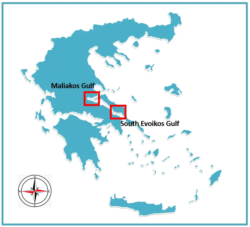
Figure 1. Location of the Maliakos and South Evoikos Gulfs, Central Greece, showing the distribution of P. radiata occurrence points (red squares). The approximate central coordinates of the Maliakos Gulf are 38.8648° N, 22.6133° E, and of the South Evoikos Gulf 38.3860° N, 23.8904° E. The inset map indicates the position of the study area in the Aegean Sea. Coordinates are given in decimal degrees (WGS 84).
2.1.2. Environmental Datasets and Predictors
Environmental predictors used in the modelling framework were obtained from the Copernicus Marine Environment Monitoring Service (CMEMS) and the European Marine Observation and Data Network (EMODnet) for the period January 2015–January 2025. These datasets describe the long-term physical, biogeochemical, and seafloor conditions of the study area and provide spatially consistent environmental information suitable for habitat-suitability modelling.
The predictor set included sea surface temperature (SST), sea bottom temperature (SBT), salinity, pH, dissolved oxygen (O2), chlorophyll-a (Chl-a), ammonium (NH4+), nitrate (NO3−), phosphate (PO43−), current velocity, bathymetry, and substrate type (Table 1). Collectively, these variables represent key physical, chemical, and habitat-related factors known to influence the spatial distribution and physiological performance of Pinctada radiata.
Table 1. Environmental parameters acquired for the Maliakos and South Evoikos Gulfs and their associated measuring units, where O2, Chl_a, NH4, NO3, and PO4 represent the concentrations of dissolved oxygen, chlorophyll-a, ammonium, nitrate, and phosphate, respectively, in the water column.
|
Parameter |
Measuring Unit |
|---|---|
|
Sea Surface Temperature (SST) |
°C |
|
Sea Bottom Temperature (SBT) |
°C |
|
Salinity |
Psu |
|
pH |
−log[H+] |
|
Dissolved Oxygen (O2) |
mmol/m−3 |
|
Chlorophyll-a (Chl_a) |
mg/m−3 |
|
Ammonium (NH4) |
mmol/m−3 |
|
Nitrate (NO3) |
mmol/m−3 |
|
Phosphate (PO4) |
mmol/m−3 |
|
Current Velocity |
m/s−1 |
|
Bathymetry |
M |
|
Substrate Type |
Categorical |
Physical oceanographic variables were sourced from the CMEMS Mediterranean multi-year physical reanalysis product (MEDSEA_MULTIYEAR_PHY_006_004), produced using the NEMO hydrodynamic model coupled with the OceanVAR data assimilation scheme and provided as monthly mean fields at an approximate spatial resolution of 4–5 km. Biogeochemical parameters were obtained from the CMEMS Mediterranean biogeochemical reanalysis (MEDSEA_MULTIYEAR_BGC_006_008), which couples the OGSTM–BFM v5.1 ecosystem model with a 3DVAR-BIO assimilation system to simulate nutrient and oxygen dynamics across the Mediterranean Sea.
Bathymetry and substrate type were derived from EMODnet Bathymetry and EMODnet Geology products, respectively, which provide higher-resolution representations of seabed morphology and sediment classes relevant to benthic habitat characterization. All environmental layers were resampled to a common 100 m grid using bilinear interpolation to ensure spatial alignment across predictors prior to modelling.
In situ hydrographic measurements collected between 2020 and 2025 were used to validate Copernicus-derived data and to confirm the environmental ranges represented by the gridded datasets. Temperature, salinity, dissolved oxygen, and pH were measured at representative nearshore and offshore stations in both gulfs using a YSI EXO2 multiparameter probe, while nutrient concentrations were determined from discrete water samples using spectrophotometric analysis. These field observations confirmed the strong hydrographic contrasts between the two systems, including frequent hypoxia and nutrient enrichment in the Maliakos Gulf and more stable, well-oxygenated mesotrophic conditions in the South Evoikos Gulf [53,54,55,56].
This issue has been clarified in the Materials and Methods section. In addition to surface-derived EO variables, we explicitly incorporated sea bottom temperature, bathymetry, and substrate type to represent near-bottom conditions experienced by this benthic species. Sea bottom temperature was derived from CMEMS physical reanalysis products and spatially matched to EMODnet bathymetry. Furthermore, in shallow semi-enclosed systems, surface variables such as SST, chlorophyll-a, and dissolved oxygen are strongly coupled to bottom conditions.
All spatial analyses, environmental harmonization, and map production were conducted using Python (v3.11) under the WGS 84/UTM Zone 34N projection.
2.2. Environmental Data Processing and Pre-Modeling Workflow
All georeferenced environmental predictors used in the modelling framework are summarized in Table 2, including their data source, product identifiers, native spatial and temporal resolution, and preprocessing steps.
All predictors were harmonized to a common 100 m grid to ensure spatial alignment and compatibility across modelling approaches. This resolution was selected as a compromise between the finger-scale coastal geomorphology represented by EMODnet products and the coarser resolution of physical reanalysis fields. However, the effective spatial resolution of the resulting suitability maps is constrained by the native resolution of the coarsest input datasets (Table 2), and resampling does not introduce new spatial information. Therefore, the 100 m grid should be interpreted as a modelling framework rather than the intrinsic resolution of all predictors.
The overall methodological workflow of the study is summarized in Figure 2. The diagram illustrates the sequential integration of Earth Observation and in situ data, environmental preprocessing and harmonization, species-occurrence bias control, multi-algorithm habitat suitability modelling, ensemble integration with explainable-AI techniques, and final model evaluation and spatial outputs.
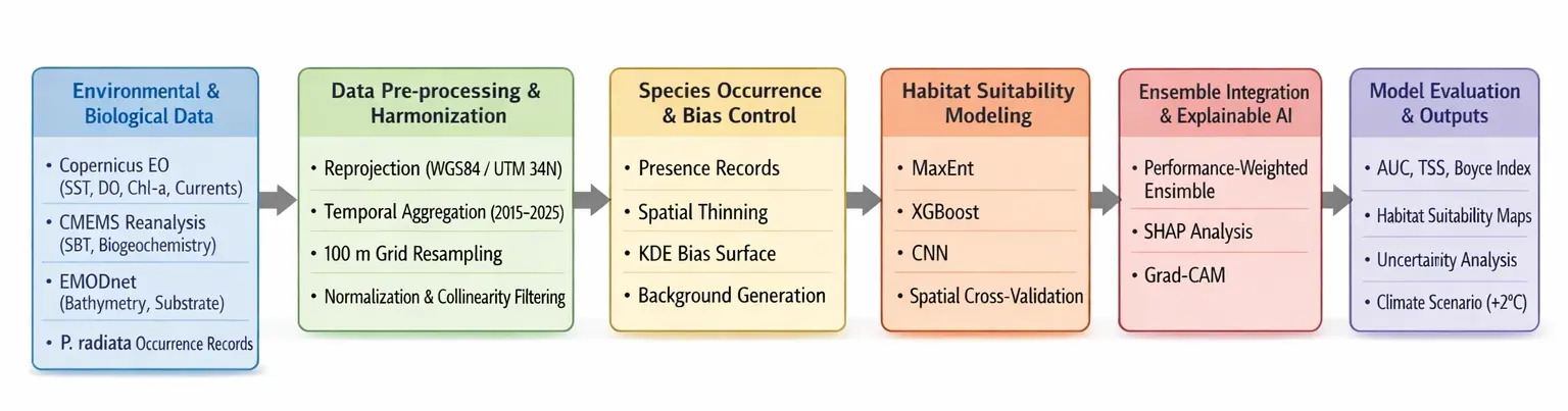
Figure 2. Technical workflow of the study illustrating data acquisition, preprocessing and harmonization, species occurrence preparation, habitat suitability modeling (MaxEnt, XGBoost, CNN), ensemble integration with explainable AI tools (SHAP, Grad-CAM), and final model evaluation and outputs.
Table 2. Environmental predictors, data sources, variable definitions, spatial resolution, temporal aggregation, and processing workflow of environmental predictors used for habitat suitability modeling of P. radiata in the Maliakos and South Evoikos Gulfs.
|
Parameter |
Source |
Product/Dataset Identifier |
Variable Name or Source |
Type (Observed/Modeled) |
Original Resolution |
Temporal Aggregation |
Access & Processing Notes |
|---|---|---|---|---|---|---|---|
|
Sea Surface Temperature (SST) |
CMEMS |
MEDSEA_MULTIYEAR_PHY_006_004 |
thetao (sea water potential temperature at depth 0 m) |
Modeled (reanalysis) |
~4–5 km, daily (2000–2025) |
Monthly climatology (2015–2025) |
Downloaded via Copernicus Marine Toolbox (Python). NetCDF CF-compliant. Bilinear resampling to 100 m. |
|
Sea Bottom Temperature (SBT) |
CMEMS |
MEDSEA_MULTIYEAR_PHY_006_004 |
thetao at sea floor |
Modeled (reanalysis) |
~4–5 km, daily (2000–2025) |
Monthly climatology (2015–2025) |
Same as SST. Depth extracted using bottomT parameter. |
|
Salinity |
CMEMS |
MEDSEA_MULTIYEAR_PHY_006_004 |
so (sea water salinity at depth 0 m) |
Modeled (reanalysis) |
~4–5 km, daily (2000–2025) |
Monthly climatology (2015–2025) |
Same as SST. |
|
pH |
CMEMS |
MEDSEA_MULTIYEAR_BGC_006_008 |
ph (sea water pH) |
Modeled (biogeochemical) |
~4–5 km, daily (2000–2025) |
Monthly climatology (2015–2025) |
Downloaded via Copernicus Marine Toolbox. Variable at surface. |
|
Dissolved Oxygen (O2) |
CMEMS |
MEDSEA_MULTIYEAR_BGC_006_008 |
O2 (mole concentration of dissolved oxygen) |
Modeled (biogeochemical) |
~4–5 km, daily (2000–2025) |
Monthly climatology (2015–2025) |
Same as pH. |
|
Chlorophyll-a (Chl-a) |
CMEMS |
MEDSEA_MULTIYEAR_BGC_006_008 |
chl (chlorophyll-a concentration) |
Modeled (biogeochemical) |
~4–5 km, daily (2000–2025) |
Monthly climatology (2015–2025) |
Same as pH. |
|
Current Velocity |
CMEMS |
MEDSEA_MULTIYEAR_PHY_006_004 |
uo (eastward velocity) and vo (northward velocity) at sea floor |
Modeled (reasonably) |
~4–5 km, daily (2000–2025) |
Monthly climatology (2015–2025) |
Magnitude calculated from uo, vo. Processed via Python xarray. |
|
Bathymetry |
EMODnet Bathymetry |
EMODnet Bathymetry DTM (2024) |
Depth (sea floor depth below sea level) |
Observed (multibeam/sounder DTMs) |
115 m (Mediterranean DTMs) |
Static (2024 release) |
Downloaded as GeoTIFF. Reprojected to WGS84/UTM34N, resampled to 100 m using bilinear interpolation. |
|
Substrate Type |
EMODnet Geology |
EMODnet Seabed Substrate 2023 |
substrate_class (Folk classification) |
Observed (grab samples, interpreted) |
1:250,000 scale |
Static (2023 release) |
Downloaded as vector layer, rasterized to 100 m grid using nearest-neighbor assignment. |
|
Ammonium (NH4) |
CMEMS (excluded) |
MEDSEA_MULTIYEAR_BGC_006_008 |
NH4 (ammonium concentration) |
Modeled (biogeochemical) |
~4–5 km, daily (2000–2025) |
Not used (collinear) |
Excluded due to collinearity with Chl-a and O2 (see Section 2.2). |
|
Nitrate (NO3−) |
CMEMS (excluded) |
MEDSEA_MULTIYEAR_BGC_006_008 |
NO3 (nitrate concentration) |
Modeled (biogeochemical) |
~4–5 km, daily (2000–2025) |
Not used (collinear) |
Excluded due to collinearity with Chl-a and O2 (see Section 2.2). |
|
Phosphate (PO43−) |
CMEMS (excluded) |
MEDSEA_MULTIYEAR_BGC_006_008 |
PO4 (phosphate concentration) |
Modeled (biogeochemical) |
~4–5 km, daily (2000–2025) |
Not used (collinear) |
Excluded due to collinearity with Chl-a and O2 (see Section 2.2). |
All environmental datasets underwent a structured preprocessing protocol designed to ensure spatial consistency, reduce multicollinearity, and optimize their integration into the habitat-suitability modeling framework. The workflow included coordinate harmonization, temporal aggregation, statistical normalization, and variable-selection procedures prior to model training (Figure 3).
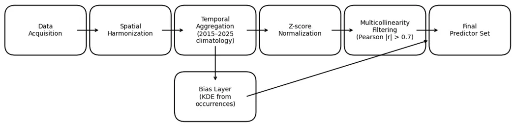
Figure 3. Workflow of environmental data preprocessing and variable selection prior to model training. Steps include spatial harmonization, temporal aggregation, z-score normalization, multicollinearity filtering, and the generation of a bias-correction layer.
Environmental layers derived from CMEMS and EMODnet products were re-projected to a common coordinate reference system (WGS 84/UTM Zone 34N) and resampled to a 100 m grid using bilinear interpolation, following established EO-based SDM preprocessing guidelines [57]. Monthly climatologies were generated for the period 2015–2025 by averaging each variable’s time series, providing stable hydrographic and biogeochemical baselines suitable for species distribution modeling by minimizing short-term variability and episodic anomalies [58,59]. Bathymetry and substrate-type rasters were harmonized to the same spatial resolution and grid alignment to ensure compatibility across datasets.
Sea bottom temperature was derived from the CMEMS Mediterranean physical reanalysis product as ‘sea water potential temperature at sea floor’, representing a modelled variable rather than a direct satellite observation. This variable corresponds to potential temperature at the deepest model layer and was spatially matched to the study bathymetry prior to harmonization.
All continuous environmental predictors were normalized using Min–Max scaling to a 0–1 range, ensuring consistent feature ranges across algorithms and facilitating stable convergence of the deep-learning (CNN) component of the ensemble. To address multicollinearity, one of the main sources of overfitting in ecological models, pairwise Pearson correlation coefficients were computed among all predictors. Variables with |r| > 0.7 were considered collinear, and only the predictor with higher ecological interpretability or stronger explanatory power in preliminary models was retained, following best practices in marine SDMs [60,61]. This procedure reduced the initial set of 13 predictors to 8 statistically independent variables representing the main environmental gradients structuring Pinctada radiata distribution in semi-enclosed Mediterranean systems.
The retained predictors included:
-
-
Sea Surface Temperature (°C) and Sea Bottom Temperature (°C), key thermal drivers influencing metabolic performance and reproductive cycles [62];
-
-
Salinity (PSU), reflecting freshwater inputs and mixing processes [63];
-
-
Dissolved Oxygen (mmol·m−3), a critical determinant of aerobic metabolism and physiological stress [64];
-
-
Chlorophyll-a (mg·m−3), a proxy for primary productivity and food availability [65];
-
-
pH (−log[H+]), indicating carbonate system equilibrium and acidification levels [66];
-
-
Current Velocity (m·s−1), representing hydrodynamic exposure and larval dispersal potential [67]; and
-
-
Bathymetry (m), describing depth constraints and benthic habitat zonation [68].
Nutrient variables (NH4+, NO3−, PO43−) were excluded due to strong collinearity with chlorophyll-a and dissolved oxygen (|r| > 0.9) and because they contributed limited unique explanatory power consistent with previous Mediterranean habitat-modelling studies where nutrient distributions covary with phytoplankton biomass and oxygen dynamics [69,70].
Sea bottom temperature was derived from the CMEMS Mediterranean physical reanalysis product (MEDSEA_MULTIYEAR_PHY_006_004) using the variable ‘sea water potential temperature at sea floor’. This variable represents modelled potential temperature at the deepest model layer and is not a direct satellite observation. For the purposes of habitat-suitability modelling, sea bottom temperature was extracted at the sea-floor level, spatially matched to EMODnet bathymetry, and used as a proxy for near-bottom thermal conditions experienced by benthic organisms.
All raster layers were clipped to the 0–90 m depth range, consistent with the known bathymetric distribution of P. radiata in the study region. Terrestrial pixels and deep offshore areas were masked. To account for sampling bias in the presence-only dataset, a kernel-density estimation (KDE) surface was generated from occurrence points and used for bias-corrected pseudo-absence selection and spatially weighted model calibration, following recommended SDM protocols for marine species [71].
The final environmental matrix consisted of eight continuous variables and one categorical predictor (substrate type). Each environmental raster was exported as a GeoTIFF file and incorporated into the AI-based ensemble modeling framework described in Section 2.3. All preprocessing operations, spatial visualization, and map production were performed in Python (v3.11) and R (v4.3) [72].
This study employed a clearly defined set of response and predictor variables, summarized conceptually below and documented in detail in Table 2 with respect to data provenance, resolution, and preprocessing.
The response variable across all modelling approaches represents habitat suitability for P. radiata. Habitat suitability was operationalized using presence-only occurrence records and background or pseudo-absence data, yielding a continuous suitability index ranging from 0 to 1. In MaxEnt, suitability was estimated from presence-only data relative to background environmental conditions. In the XGBoost and CNN models, presence locations were contrasted with pseudo-absence/background samples to learn a continuous suitability function across environmental gradients.
Independent variables consisted of environmental predictors describing thermal conditions (sea surface and bottom temperatures), hydrography (salinity, current velocity), biogeochemistry (dissolved oxygen, chlorophyll-a, pH), and seafloor characteristics (bathymetry and substrate type). These variables represent key physical, chemical, and habitat-related drivers known to influence the distribution and physiological performance of benthic suspension feeders.
All predictors were obtained from Copernicus Marine Environment Monitoring Service (CMEMS) and EMODnet products, including both directly observed (satellite and in situ–derived) variables and modelled or reanalysis fields, as specified in Table 2. Native spatial resolutions ranged from kilometer-scale reanalysis products to finer-resolution EMODnet layers, while temporal resolution varied from monthly fields to static seabed datasets.
Prior to modelling, all predictors were harmonized to a common 100 m grid, temporally aggregated into 2015–2025 climatologies, and clipped to the accessible depth range of the species (0–90 m). Continuous variables were normalized using min–max scaling (0–1). The categorical substrate variable was encoded using one-hot (dummy) encoding for machine-learning and deep-learning models. Predictor collinearity was assessed using Pearson correlation coefficients and variance inflation factors, yielding a final set of eight independent continuous predictors and one categorical variable, consistently used across all models.
2.3. Species Occurrence Data and Spatial Bias Control
Presence records of P. radiata were compiled from systematic field surveys carried out between 2015 and 2025 in the Maliakos and South Evoikos Gulfs, as part of regional monitoring programs on benthic biodiversity and aquaculture-site evaluations. Additional confirmed occurrences were retrieved from institutional databases (HCMR, EMODnet Biology) and from published studies documenting populations of the species in the Aegean Sea [73,74,75]. All records were subjected to detailed taxonomic and geospatial checks. Coordinates were verified against high-resolution coastline and bathymetry datasets, and duplicate or unreliable entries (e.g., points falling on land, inside ports, or outside the known depth range of the species) were removed. To reduce spatial clustering relative to the modelling grid, the dataset was thinned using a minimum nearest-neighbor distance of 500 m.
Species distribution was modelled using MaxEnt (Maximum Entropy), a machine-learning algorithm widely used in species distribution modelling with presence-only data, where pseudo-absence or background points are used to characterize the available environmental space, together with XGBoost and a convolutional neural network (CNN).
Because presence-only records often reflect uneven sampling effort, we constructed a sampling-bias surface using Kernel Density Estimation (KDE) applied to the thinned dataset [76]. The KDE bandwidth was estimated following Silverman’s rule of thumb and matched to the 100-m modelling grid, allowing broad sampling trends to be captured without reproducing fine-scale survey hotspots. This KDE surface was then used as a weighting layer for selecting 10,000 background (pseudo-absence) points. Weighting background selection according to sampling intensity is an important step in presence-only SDMs to avoid bias introduced by uneven survey effort [77].
Background points were generated within the accessible marine area (M) of P. radiata, defined here as the 0–90 m depth zone encompassing the two gulfs and extended with a 2-km offshore buffer. Only marine cells were retained. KDE-weighted sampling helped prevent oversampling either intensively surveyed zones or areas with little to no sampling.
The set of predictor variables used in the modelling corresponds to the multicollinearity-filtered subset derived in Section 2.2. In brief, continuous variables were examined using pairwise Pearson correlations (|r| > 0.7) and the Variance Inflation Factor (VIF < 5), following common practice in ecological modelling [78,79,80]. This screening yielded a final group of eight statistically independent continuous predictors and one categorical substrate class.
All continuous predictors had been previously normalized using min–max scaling (0–1) to maintain similar feature magnitudes and support stable convergence across all machine-learning algorithms, including the CNN. The categorical substrate variable was encoded using one-hot dummy coding to avoid imposing any artificial ordering among substrate types.
Dataset sufficiency was assessed using the Sample-size to Feature-size Ratio (SFR):
|
```latexSFR=\frac{{N}_{\text{samples}}}{{N}_{\text{features}}}``` |
(1) |
Values above 10 indicate adequate sample density for machine-learning models [81]. In this study, 220 validated presence points and eight independent predictors yielded an SFR of 27.5, exceeding recommended thresholds.
The response variable in all modelling approaches represents habitat suitability, operationalized using presence-only occurrence records of Pinctada radiata and background or pseudo-absence data. In MaxEnt, suitability is estimated as a continuous probability surface based on presence-only and background data. For XGBoost and CNN models, presence points were contrasted with pseudo-absence/background samples to learn a continuous suitability function across environmental gradients.
Spatial autocorrelation among occurrences was assessed using Moran’s I. The resulting value (I = 0.07, p = 0.38) indicated no significant clustering, satisfying independence assumptions for model training [82,83]. The finalized dataset, comprising KDE-weighted presence and background points and the multicollinearity-filtered predictor set, served as the basis for the ensemble habitat-suitability modelling framework.
The response variable in all modelling approaches represents habitat suitability for P. radiata, operationalized using presence-only occurrence records and background or pseudo-absence data. In MaxEnt, suitability is estimated as a continuous surface derived from presence-only data relative to background environmental conditions. For XGBoost and CNN models, presence locations were contrasted with pseudo-absence/background samples to learn a continuous suitability function across environmental gradients. All environmental predictors retained after multicollinearity filtering (Section 2.2; Table 2) were used consistently across the three models. Continuous predictors were normalized prior to modelling, while the categorical substrate variable was encoded using one-hot (dummy) encoding for XGBoost and CNN.
2.4. Ensemble Species Distribution Modeling Framework
To model the habitat suitability of P. radiata across the Maliakos and South Evoikos Gulfs, we developed a multi-algorithm ensemble framework integrating three complementary approaches: Maximum Entropy (MaxEnt), Extreme Gradient Boosting (XGBoost), and Convolutional Neural Networks (CNN). Each algorithm offers distinct strengths: MaxEnt is optimized for presence-only ecological datasets, XGBoost captures nonlinear predictor interactions with strong regularization, and CNNs exploit spatial structure encoded in gridded environmental layers. Combining these models reduces individual biases, enhances predictive robustness, and generates ecologically coherent suitability surfaces in heterogeneous coastal environments [84,85,86].
The robustness of the modeling framework was enhanced through a rigorous data-cleaning and bias-correction workflow (Figure 4). To address the spatial clustering of P. radiata records, which could lead to model overfitting, we implemented a spatial thinning protocol (Figure 4B). This ensured that a single occurrence was retained within a 100 m grid cell, effectively reducing spatial autocorrelation. Simultaneously, to account for sampling bias, a Kernel Density Estimation (KDE) surface was generated to represent the intensity of the sampling effort (Figure 4C). This surface was utilized to weigh the selection of background points, ensuring that the AI models distinguish between ecological suitability and sampling accessibility. Finally, all presence points (n = 220) were geographically audited to ensure they were strictly positioned in marine environments, specifically covering the bathymetric gradients from the Maliakos Gulf to the southern Aliveri sector (Figure 4A).
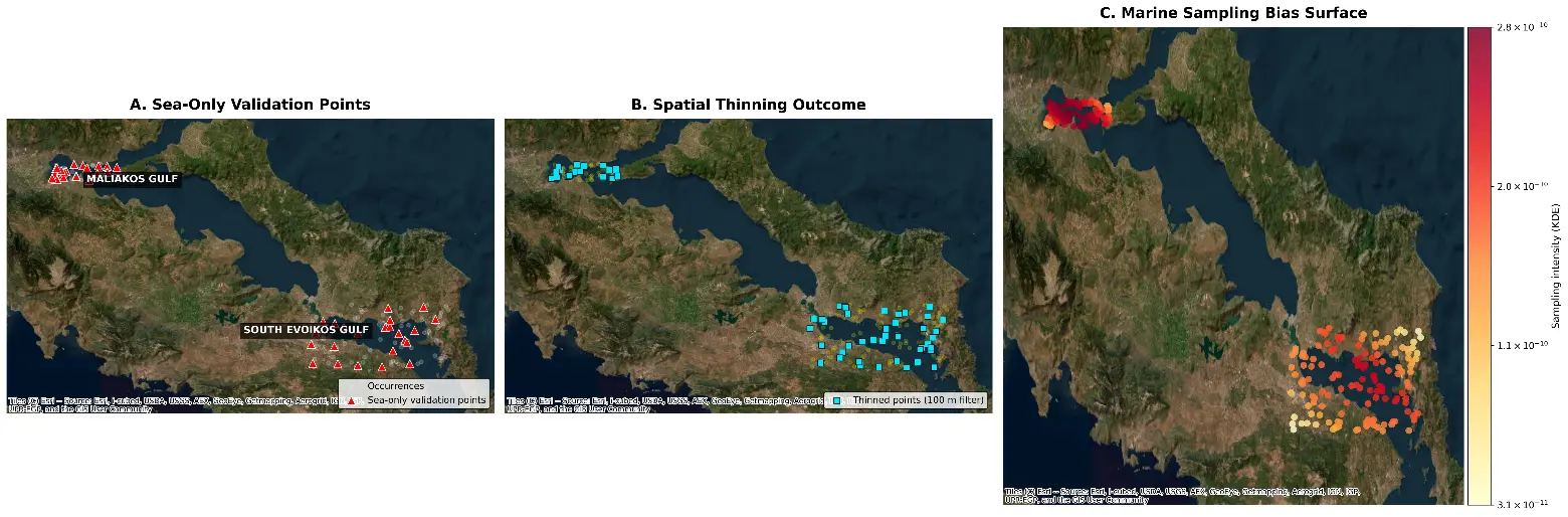
Figure 4. Geospatial documentation and data preprocessing stages for the habitat suitability modeling of P. radiata. (A) In-situ validation stations showing the spatial distribution of field sampling stations (2020–2025) within the Maliakos and South Evoikos Gulfs. Red triangles indicate the validated occurrence points retained exclusively in the marine environment, ensuring the geographical precision of the independent model validation process. (B) Spatial thinning outcome showing the filtered presence dataset after application of a 100 m grid-based thinning procedure. Cyan squares indicate the retained occurrence points after thinning, a step used to reduce spatial autocorrelation and mitigate model overfitting in areas with disproportionately high sampling density. (C) Sampling bias surface derived from kernel density estimation (KDE), representing spatial variation in sampling effort. Warmer colors indicate higher sampling intensity, whereas lighter colors indicate lower sampling intensity. This surface was used to guide the selection of background points (pseudo-absences), allowing the AI models to distinguish true environmental suitability from non-random sampling effort along the coastal zone.
2.4.1. MaxEnt Modeling
MaxEnt was implemented using the maxnet package in R, following established guidelines for presence-only SDMs [87]. Model tuning was performed via five-fold environmental block cross-validation and included testing of multiple regularization multipliers (0.5–5) and feature classes (linear, quadratic, hinge). The optimal configuration was selected using the Akaike Information Criterion corrected for small samples (AICc), ensuring an appropriate balance between model fitness and complexity.
The final model produced continuous suitability estimates using the cloglog transformation, which yields values interpretable as relative occurrence rates rather than true probabilities of presence. Variable influence was assessed using permutation importance and Jackknife tests, allowing clear identification of the predictors most strongly shaping the realized niche of P. radiata.
2.4.2. Extreme Gradient Boosting (XGBoost)
The XGBoost model was implemented in Python using the xgboost library. Hyperparameter tuning used a grid search across learning rate, maximum tree depth, and number of boosting rounds, combined with environmental block cross-validation to avoid inflated accuracy due to spatial autocorrelation. The final model used a learning rate of 0.05, a maximum depth of 6, and 300 boosting iterations. To correct for sampling bias, KDE-derived sampling weights (from Section 2.3) were applied to both presence and background points. Predictive uncertainty was quantified through bootstrap resampling (n = 100), generating ensemble means suitability predictions and pixel-level uncertainty layers that reflect variability in tree-based model outcomes [88].
2.4.3. Convolutional Neural Network (CNN)
A CNN was implemented in TensorFlow/Keras to incorporate spatial context from environmental rasters explicitly. For each presence and pseudo-absence point, a 32 × 32-cell environmental patch (~3.2 × 3.2 km) was extracted from all normalized predictors. This scale corresponds to meso-scale gradients of temperature, salinity, oxygen, and current velocity in semi-enclosed gulfs and matches the benthic dispersal processes relevant to low-mobility bivalves [89]. Each environmental predictor formed a separate input channel.
The CNN architecture consisted of three convolutional layers (3 × 3 filters) with ReLU activation, batch normalization, dropout (0.3), followed by two fully connected layers and a final sigmoid output. Training used the Adam optimizer (learning rate = 0.0001) and binary cross-entropy loss, with early stopping to prevent overfitting.
To prevent spatial leakage, a key issue in CNN-based SDMs, environmental block cross-validation was applied [90]. Mild data augmentation (rotations and reflections) was used to improve generalization while avoiding ecologically unrealistic distortions.
2.4.4. Ensemble Integration
Predictions from the three models were combined using a performance-weighted ensemble, where each algorithm’s contribution was proportional to its mean cross-validated Area Under the Curve (AUC). The ensemble suitability score (E) was computed as:
|
```latexE=\sum _{i=1}^{n}{w}_{i}{P}_{i}``` |
(2) |
where $${P}_{i}$$ is the normalized suitability output of model $$i$$, and $${w}_{i}$$ is its the AUC-derived weight such that $$\sum {w}_{i}=1$$.
Ensemble weights were not treated as user-defined or tunable hyperparameters to avoid subjective bias and ensure that model contributions reflect objective predictive performance.
This strategy integrates the complementary strengths of the algorithms, allocating greater weight to higher-performing models while retaining the spatial and ecological diversity of all three approaches. Performance-weighted ensembles are widely shown to outperform individual models, especially in coastal and marine systems where environmental gradients are nonlinear and spatially heterogeneous [91,92].
2.5. Model Evaluation and Statistical Validation
Model performance was evaluated using a spatially explicit framework designed to limit the influence of spatial autocorrelation and provide reliable estimates of generalization across the two study areas. To do this, presence and background records were divided into five spatially stratified folds using an environmental-blocking approach implemented with the blockCV methodology [93]. The procedure groups grid cells according to environmental similarity and geographic proximity, producing training and validation sets that are both spatially independent and environmentally distinct. Each fold was used in turn as the validation subset, with the remaining folds assigned to model training.
A combination of evaluation metrics was applied to capture different aspects of predictive accuracy and ecological realism. The Area Under the Receiver Operating Characteristic Curve (AUC) was used as a general measure of discrimination, while the True Skill Statistic (TSS) provided a threshold-dependent metric balancing sensitivity and specificity. Threshold selection followed the “maximum sensitivity plus specificity” criterion. Because presence–background models are sensitive to varying prevalence, we also calculated the Area Under the Precision–Recall Curve (AUC-PR), which is more informative under low-prevalence conditions. Ecological calibration was assessed through the Continuous Boyce Index (CBI), which evaluates how well model predictions reflect the empirical distribution of presences along the suitability gradient and is widely used in SDM validation [94,95].
To compare performance across algorithms, fold-level AUC scores were tested using the two-sided DeLong test, a non-parametric method suitable for correlated ROC curves [94]. Fold-specific values were used to maintain statistical independence. We further assessed spatial autocorrelation in residuals from spatial cross-validation using Moran’s I with an inverse-distance weighting scheme. No significant autocorrelation was detected (p > 0.05 for all models), confirming that the blocking procedure effectively reduced spatial dependence between training and testing sets.
Inter-model agreement was examined using Pearson’s correlation for continuous suitability outputs and Cohen’s κ for binary classifications based on the optimal threshold. κ was interpreted following recent guidelines, with values above 0.6 considered strong agreement. Spatial mismatches in model outputs were mapped to identify areas where environmental gradients were interpreted differently across algorithms. Model accuracy and validation are now described in detail. We evaluated model performance using spatial block cross-validation and multiple complementary metrics, including AUC, TSS, AUC-PR, and the Continuous Boyce Index. The habitat suitability index is defined as a continuous 0–1 measure derived from presence and background data, and its robustness is demonstrated through ensemble performance, inter-model agreement, and bootstrap uncertainty analysis.
Prediction uncertainty was quantified using a bootstrap resampling approach. For each algorithm, 100 bootstrap iterations were run by resampling presence and background points with replacement and re-fitting the model. From these iterations, mean suitability and standard deviation (σ) rasters were generated, allowing the identification of areas with high predictive uncertainty. Regions with σ values in the upper quartile were treated as uncertainty hotspots, typically associated with transitional environments, weaker or conflicting gradients, or lower sampling intensity.
All statistical analyses were carried out in R (v4.3) using the blockCV, pROC, and SDMTools packages, and in Python (v3.10) using scikit-learn, numpy, and scipy.
2.6. Explainable AI and Model Interpretability
Interpreting how environmental predictors influence species-distribution outcomes is essential for evaluating the ecological soundness of machine-learning models. To address this, we applied a structured explainability framework informed by recent developments in interpretable ecological modelling [96]. The aim was to capture both the statistical contribution of individual variables and the spatial features that support predicted habitat suitability for P. radiata.
For the MaxEnt model, interpretability was examined through permutation importance and Jackknife tests of model gain, calculated across spatially independent folds. These diagnostics help assess the relative influence of each predictor and reveal how combinations of variables contribute to model gain, while partly accounting for correlations among predictors [97,98]. In addition, response curves with 95% confidence envelopes were generated for key variables, allowing nonlinear responses in temperature, salinity, dissolved oxygen, and substrate to be visualized.
For the XGBoost algorithm, we used TreeSHAP, an exact method for deriving feature contributions in tree-based models [97,98,99]. SHAP values were computed using validation folds to avoid inflating importance estimates. Global explanations and dependence plots highlighted nonlinear and interaction effects, for instance, reduced suitability at high sea temperatures or under low oxygen conditions, patterns that match known physiological constraints of P. radiata. To reduce interpretational bias from predictor collinearity, SHAP interaction values were also reviewed, ensuring that the strongest predictors retained independent explanatory value [100,101,102].
Model interpretability was assessed using SHAP (SHapley Additive exPlanations), an explainable AI method that quantifies the contribution of each predictor to individual model predictions.
Interpretation of the CNN relied on Gradient-weighted Class Activation Mapping (Grad-CAM), which identifies the portions of the input most relevant to the model’s output [100,102]. Grad-CAM maps were produced for both presence and pseudo-absence tiles across all validation folds, providing a consistency check for the CNN’s spatial attention. The maps recurrently emphasized shallow, sheltered coastal areas habitats already known to favor benthic suspension feeders, indicating that the CNN was responding to ecologically meaningful features rather than artefacts of the training procedure. The effect of data augmentation (rotations and reflections) on spatial attention was also examined to verify that Grad-CAM patterns remained stable.
Finally, we compared interpretability outputs from the three modelling approaches to identify shared ecological signals. The alignment among SHAP-based attributions, MaxEnt Jackknife results, and Grad-CAM spatial patterns provided a coherent, multi-angle interpretability framework consistent with current standards in explainable AI for ecology [98,103]. Across all models, sea temperature, dissolved oxygen, substrate type, and current velocity emerged as the most influential predictors of suitable habitat. This consistency strengthens confidence in the ensemble predictions and supports the ecological relevance of the suitability patterns identified in the semi-enclosed systems of the region. For the tree-based XGBoost model, we applied TreeSHAP, an exact and computationally efficient SHAP implementation specifically designed for ensemble tree methods
2.7. Spatial Mapping and Uncertainty Analysis
Ensemble suitability predictions were expressed on a continuous 0–1 scale and subsequently grouped into suitability classes using a thresholding approach based on statistical optimization rather than fixed numerical cutoffs. Suitability categories were defined using the threshold that maximized the True Skill Statistic (TSS), in combination with the 10th-percentile training-presence rule, a commonly applied criterion in presence-only and machine-learning SDMs [104,105]. This approach produced three classes: low, moderate, and high suitability while maintaining ecological interpretability and limiting bias associated with arbitrary thresholds.
Predictive uncertainty was quantified using a spatial block bootstrap with 100 replicates for each of the three base models. Resampling at the block level, instead of at individual points, accounts for the spatial autocorrelation inherent in both environmental predictors and species-occurrence data and follows current recommendations for marine SDMs [106]. For each algorithm, we calculated the mean, standard deviation (σ), and coefficient of variation (CV) across replicates. Areas exceeding the 90th percentile of σ were treated as high-uncertainty zones, a criterion that reflects the structure of model-derived error rather than an arbitrary boundary [107]. These zones were concentrated around freshwater-dominated coastal areas and in regions with sharp bathymetric or hydrodynamic gradients, where environmental heterogeneity and data variability are highest.
Inter-model agreement among MaxEnt, XGBoost, and the CNN was assessed using several complementary metrics to avoid relying on a single measure of similarity. Pairwise spatial agreement was evaluated using Pearson’s r, the Continuous Boyce Similarity Index, and Cohen’s κ computed from threshold-based binary maps [108]. κ values were interpreted following Landis and Koch (1977) only after verifying that thresholding did not introduce systematic bias. Overall agreement was high (r = 0.84; κ = 0.73), indicating that the three algorithms converged toward similar spatial patterns despite their methodological differences. In addition, the Sørensen spatial overlap index was used to quantify the extent to which high-suitability areas overlapped across models, a metric that has gained traction in ensemble SDMs due to its relative insensitivity to prevalence [109].
Spatial autocorrelation in prediction residuals was examined using Moran’s I with a 2-km distance threshold. The absence of significant autocorrelation indicated that the spatial cross-validation framework effectively reduced spatial dependence during model evaluation [110], a critical step in marine systems where gradients in temperature, salinity and nutrients can otherwise lead to over-optimistic performance estimates.
Thematic control and visual hierarchy in suitability mapping followed established cartographic principles as described. The selection of sequential color ramps was based on perceptual uniformity and monotonic data progression, ensuring that higher suitability values were visually emphasized without introducing artificial discontinuities. Legend design, class interval structure, and spatial emphasis were calibrated to preserve ecological gradients while maintaining interpretability and visual balance. This approach ensured that cartographic representation supported analytical interpretation rather than distorting it.
Finally, the weighted ensemble map was generated by integrating the three models using the performance-based weighting scheme outlined in Section 2.4.4. The final composite surface highlights areas where the three algorithms consistently predicted high suitability, while incorporating uncertainty layers to draw attention to regions where predictions should be interpreted cautiously. This combined representation of suitability and uncertainty supports more reliable ecological interpretation, improves transparency for management applications, and aligns with recent recommendations for predictive habitat modelling in coastal and semi-enclosed marine environments [111,112,113].
2.8. Reproducibility and Data Availability
All data handling, analytical workflows, and model configurations were developed in accordance with the FAIR principles (Findable, Accessible, Interoperable, and Reusable) to ensure transparency and reproducibility throughout the study [114]. Environmental datasets were sourced from the Copernicus Marine Environment Monitoring Service (CMEMS) and the Copernicus Land Monitoring Service (CLMS), using the most recent multi-year reanalysis products available as of January 2025. Each dataset retains its original DOI, service identifiers, and version metadata so that future updates can be fully traced [115].
Environmental predictors, including SST, SBT, salinity, dissolved oxygen, pH, chlorophyll-a, current velocity, bathymetry, and substrate type, were processed within a standardized geospatial framework to ensure spatial consistency, traceability, and reproducibility [116,117]. Raster layers were resampled to a common 100-m grid using bilinear interpolation for continuous variables and nearest-neighbor interpolation for categorical variables. Temporal climatologies for the period 2015–2025 were generated using reproducible scripts, all of which were archived under version control.
Modelling workflows, including preprocessing steps, correlation screening, MaxEnt settings, XGBoost hyperparameter tuning, the definition of the CNN architecture, and ensemble integration, were carried out in R (v4.3) and Python (v3.10). Full documentation of software versions, dependencies, and parameter choices is available in an accompanying GitHub repository (a public link will be released upon publication). To support long-term reproducibility, all computational environments were encapsulated in Docker containers, including specifications for CPU/GPU requirements, the CUDA drivers used during CNN training, and operating system dependencies [118,119,120].
Occurrence records, sampling-bias layers, final suitability rasters, and cross-validation outputs will be archived in Zenodo, an open-access repository, with a DOI assigned upon publication. Sensitive locations associated with aquaculture facilities or restricted zones were spatially masked in line with best practices for open ecological data [121]. Deposited datasets are accompanied by metadata describing projection systems, uncertainty estimates, random seeds, and workflow provenance, following widely adopted guidelines for reproducible ecological research [122].
By combining open-access datasets, explicit versioning, containerized environments, and comprehensive documentation of analytical steps, this study ensures that all results can be independently replicated, re-evaluated, or expanded by researchers working on marine habitat modelling, biodiversity assessment, or environmental forecasting. While climatological averages provide robust baselines, they may under-represent short-lived extreme events such as acute hypoxia or marine heatwaves.
All cartographic outputs were re-evaluated prior to final compilation. Raster layers were checked for projection consistency (WGS 84/UTM Zone 34N), grid alignment, and spatial resolution harmonization. Layer stacking and overlay procedures were verified to prevent pixel shifts or misalignment artifacts. Legend structure, color ramps, and class intervals were standardized to ensure thematic consistency across all figures. Scale bars and orientation elements were recalibrated following final projection validation.
3. Results
3.1. Model Performance and Predictive Accuracy
The ensemble modelling framework integrating MaxEnt, XGBoost, and a Convolutional Neural Network (CNN) demonstrated consistently high predictive performance across both gulfs. Spatial block five-fold cross-validation showed that all three algorithms achieved strong discrimination capacity, although with clear differences in predictive strength. The CNN performed best (AUC = 0.93 ± 0.02), followed by XGBoost (AUC = 0.91 ± 0.03). MaxEnt produced slightly lower values (AUC = 0.89 ± 0.04), a pattern consistent with its more constrained ability to capture complex nonlinear interactions.
When integrated into a performance-weighted ensemble, predictive accuracy improved further, yielding an AUC of 0.94 ± 0.01 and a TSS of 0.80 ± 0.02. These metrics indicate that the ensemble effectively combined the complementary strengths of the individual algorithms, resulting in lower variance and more stable predictions. Precision–recall performance (AUC-PR = 0.92) and a high Boyce Index (0.83) further support the ensemble’s strong generalization capacity within the spatially heterogeneous coastal environments of the study area.
A two-sided DeLong test confirmed that the CNN significantly outperformed MaxEnt (p = 0.038), while its improvement over XGBoost, although positive, was not statistically significant (p = 0.081). Residual spatial autocorrelation in ensemble predictions was low (Moran’s I = 0.06, p = 0.41), indicating that spatial blocking effectively reduced spatial structure in model residuals. Table 3 summarizes the comparative performance metrics across all algorithms. The ensemble consistently showed the highest predictive accuracy and the lowest across-fold variance.
Table 3. Mean performance metrics (±SD) for the three individual models and the ensemble, based on five-fold spatial cross-validation (AUC, Area Under the Curve; TSS, True Skill Statistic; AUC-PR, Area Under the Precision–Recall Curve, CBI, Continuous Boyce Index). The ensemble achieved the highest overall accuracy and lowest variance.
|
Model |
AUC (±SD) |
TSS (±SD) |
AUC-PR |
CBI |
|---|---|---|---|---|
|
MaxEnt |
0.89 ± 0.04 |
0.71 ± 0.05 |
0.85 |
0.76 |
|
XGBoost |
0.91 ± 0.03 |
0.74 ± 0.04 |
0.88 |
0.79 |
|
CNN |
0.93 ± 0.02 |
0.78 ± 0.03 |
0.91 |
0.81 |
|
Ensemble |
0.94 ± 0.01 |
0.80 ± 0.02 |
0.92 |
0.83 |
The comparative performance metrics presented in Table 3 highlight the clear improvement achieved through ensemble integration, particularly in terms of predictive stability and discrimination capacity. To further illustrate these differences across modelling approaches, Figure 5 provides a visual comparison of AUC and TSS values among the three individual algorithms and the ensemble model. This graphical summary underscores the consistent advantage of the ensemble, which not only outperformed each constituent model but also exhibited the lowest variability across validation folds.
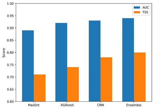
Figure 5. Performance comparison of MaxEnt, XGBoost, CNN, and the ensemble model. Bars show mean AUC (blue) and TSS (orange) values from five-fold spatial cross-validation. The ensemble model achieved the highest overall performance, confirming the benefit of integrating multiple algorithms.
3.2. Spatial Patterns of Habitat Suitability
The ensemble habitat-suitability predictions revealed clear and ecologically coherent spatial patterns across both study areas (Figure 6). In the Maliakos Gulf, high-suitability zones (≥0.7) were primarily concentrated in the shallow central basin and along the western coastal shelf between approximately 10 and 25 m depth. These areas are characterized by low-energy hydrodynamic conditions (<0.15 m·s−1), fine-grained sediments, and moderate chlorophyll-a concentrations, environmental attributes that collectively indicate stable benthic conditions favourable to Pinctada radiata. Moderate suitability (0.4–0.7) extended toward the mouth of the Spercheios River, where increased salinity variability and nutrient inputs generate pronounced environmental heterogeneity. In contrast, deeper locations (>25 m) and sectors exposed to strong currents (>0.25 m·s−1) were consistently classified as low suitability (<0.3), reflecting reduced substrate stability and heightened hydrodynamic stress.
In the South Evoikos Gulf, the highest suitability values were identified along sheltered western and southern embayments dominated by sandy–muddy substrates, moderate bottom-current velocities (0.1–0.2 m·s−1), and well-oxygenated near-bottom waters. These areas coincide with soft-sediment benthic communities and, in several cases, are located in proximity to Posidonia oceanica meadows. Although the model does not explicitly incorporate seagrass structural attributes, the spatial alignment between high-suitability zones and these habitats is consistent with the stabilizing influence of seagrass meadows on sediment dynamics. Offshore regions deeper than ~60 m and areas subject to persistent high-energy conditions (>0.3 m·s−1) were consistently assigned low suitability, in agreement with the species’ known affinity for shallow, low-energy coastal environments.
Across both gulfs, the spatial distribution of suitability closely followed the dominant environmental gradients identified through explainable-AI analyses. Bottom temperature, dissolved oxygen, and substrate type emerged as the principal drivers shaping suitable habitat, while hydrodynamic exposure was the key factor limiting suitability in offshore areas. The strong correspondence between predicted suitability patterns and independent environmental gradients supports the ecological realism of the results and underscores their utility for habitat characterization in semi-enclosed Mediterranean systems.
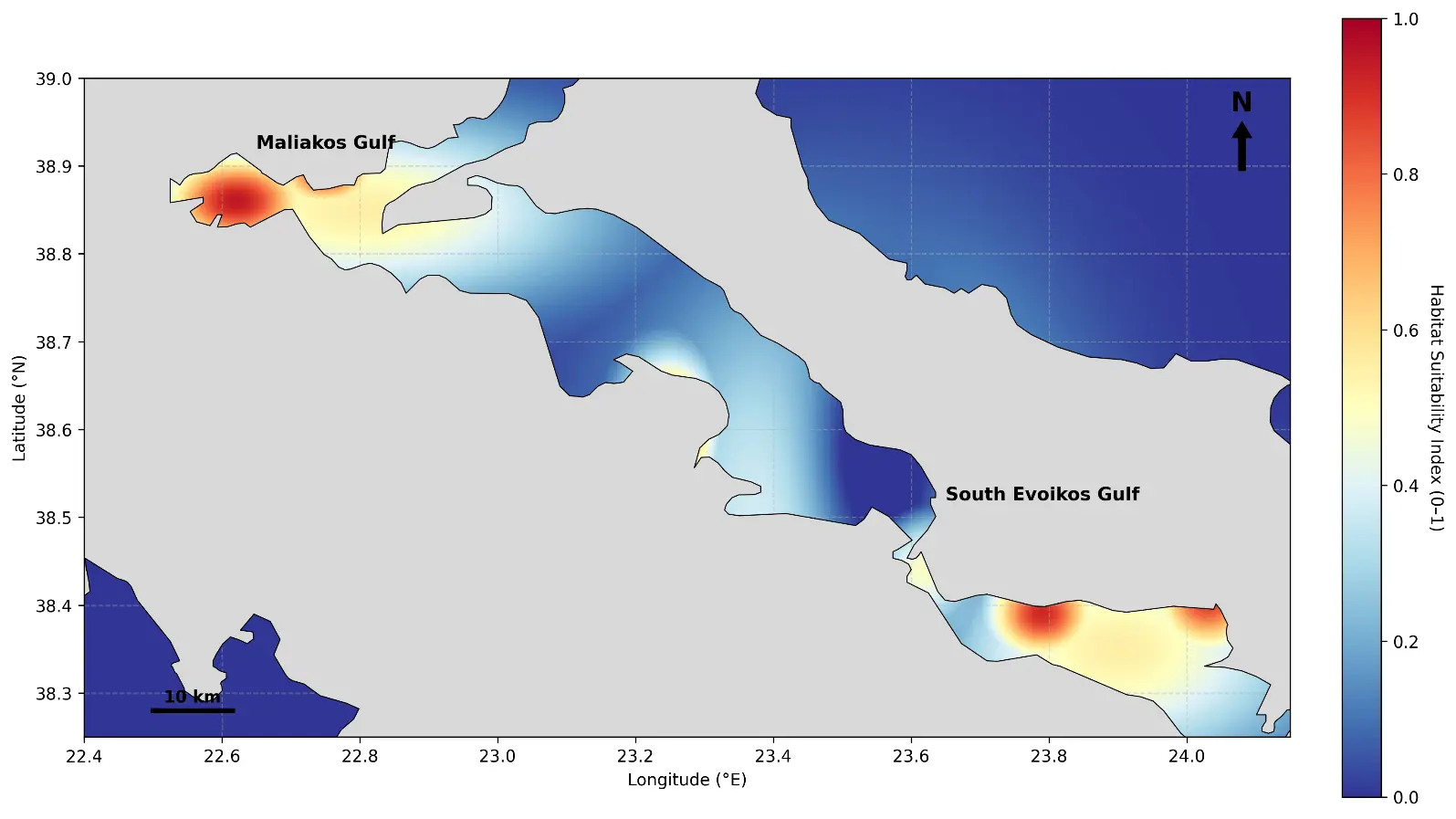
Figure 6. Predicted habitat suitability map for Pinctada radiata in the Maliakos and Evoikos Gulfs based on the ensemble model. The color scale indicates the suitability index (0–1), where warm colors (red) represent high-suitability zones (index ≥ 0.7) concentrated in the shallow central basin of Maliakos and sheltered western embayments of South Evoikos. Cool colors (blue) denote low-suitability areas associated with deeper waters (>60 m) and higher hydrodynamic exposure. Land areas are masked in gray.
3.3. Environmental Drivers of Distribution
Explainable-AI analyses provided a coherent view of the environmental gradients shaping the predicted distribution of Pinctada radiata across the two study systems. SHAP values derived from the XGBoost model and SHAP-consistent attribution patterns extracted from the CNN indicated that sea surface temperature (SST), dissolved oxygen (DO), and substrate type were the most influential predictors (Table 4). These variables exhibited strong individual contributions and consistent interaction effects, highlighting their joint role in structuring habitat suitability.
Table 4. Relative importance of environmental predictors derived from SHAP analyses and their ecological interpretation. The values represent mean normalized |SHAP| contributions across all cross-validation folds.
|
Variable |
Mean SHAP Importance |
Direction of Effect |
Ecological Interpretation |
|---|---|---|---|
|
Sea Surface Temperature (SST) |
0.27 |
Optimum 20–26 °C; sharp decline >27 °C |
Thermal tolerance and metabolic optimum |
|
Dissolved Oxygen (DO) |
0.25 |
Positive >6 mg·L−1; strong negative <4 mg·L−1 |
Oxygen limitation; hypoxia avoidance |
|
Substrate Type |
0.23 |
Highest for sandy–muddy and Posidonia substrates |
Attachment stability; food retention |
|
Chlorophyll-a |
0.18 |
Optimum at 1–3 mg·m−3 |
Mesotrophic productivity as feeding support |
|
Bathymetry |
0.14 |
Peak at 5–25 m |
Depth-related hydrodynamic and light constraints |
|
Current velocity |
−0.12 |
Negative >0.25 m·s−1 |
Hydrodynamic stress; dislodgement risk |
SST showed the highest relative importance. SHAP dependence curves indicated that suitability increased within a temperature range of approximately 20–26 °C and declined sharply above ~27 °C. These patterns align with reported thermal tolerances for the species in the Eastern Mediterranean and were reproduced across cross-validation folds, suggesting a stable and robust temperature response.
Dissolved oxygen was the second most influential predictor. Suitability increased under well-oxygenated conditions (>6 mg·L−1), while strong negative contributions occurred below ~4 mg·L−1 consistent with bivalve sensitivity to hypoxia. Joint SHAP analyses indicated that the influence of low DO strengthens at higher SST levels, revealing a combined thermal–oxygen stress effect that is characteristic of stratified summer conditions in semi-enclosed basins such as Maliakos.
Substrate type also exerted a substantial influence. Sandy–muddy sediments and areas adjacent to Posidonia oceanica meadows showed positive contributions, whereas coarse substrates and steeply sloping bottoms yielded negative SHAP values. These patterns are consistent with the species’ association with stable, fine-grained substrates. Interaction analyses further showed that the positive effect of suitable substrates weakened when bottom-current velocities exceeded ~0.25 m·s−1, underscoring the importance of low-energy benthic environments for attachment and feeding.
Chlorophyll-a contributed moderately, with maximum suitability occurring around 1–3 mg·m−3, reflecting mesotrophic conditions typical of semi-enclosed coastal systems. Bathymetry exhibited a well-defined additive effect, with the highest suitability between approximately 5 and 25 m depth. Depth also modulated the effects of SST and DO, as deeper cells became unsuitable under stratified summer conditions in the Maliakos Gulf.
Grad-CAM visualizations from the CNN provided complementary spatial indications of the influence of the predictors. High-activation areas correspond primarily to sheltered nearshore environments characterized by low hydrodynamic exposure and fine sediment. Although CNN attributions operate at the patch level rather than the pixel level, the observed activation patterns were spatially consistent with the environmental gradients inferred from SHAP analyses. Differences between the two gulfs were also evident: activation patterns in Maliakos were more spatially constrained, reflecting strong riverine and seasonal oxygen gradients, while those in South Evoikos were more diffuse and aligned with its more stable hydrodynamic regime.
Together, the SHAP and CNN attribution results indicate that the ensemble model captured ecologically meaningful gradients rather than artefacts of model structure or sampling. The consistency of key thresholds across algorithms and validation folds, combined with the alignment of spatial attribution patterns with known habitat characteristics, supports the ecological realism and interpretability of the predicted suitability patterns.
The relative contributions presented in Table 3 indicate that thermal conditions, oxygen availability, and substrate composition exert the strongest influence on the spatial distribution of P. radiata. These patterns were consistently reproduced across all ensemble components, suggesting that the model captured biologically meaningful gradients rather than statistical artefacts. To further illustrate these relationships, Figure 7 visualizes the SHAP-inspired importance scores derived from the CNN and ensemble models. The plot highlights clear separation among predictor groups, with SST and dissolved oxygen emerging as dominant drivers, followed by substrate and chlorophyll-a, whereas bathymetry and current velocity exert more localized, secondary effects. Together, these results confirm the ecological coherence of the model and provide a robust basis for interpreting habitat suitability across the two semi-enclosed systems.
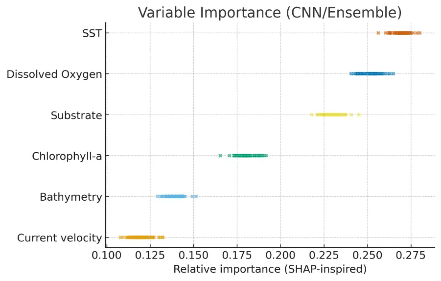
Figure 7. Relative importance of environmental predictors based on SHAP analyses and Grad-CAM activation patterns from the CNN model. Warmer colors denote stronger influence. SST, DO, and substrate type consistently emerged as the most influential drivers, reflecting the species’ preference for warm, well-oxygenated, low-energy coastal environments.
3.4. Model Agreement and Uncertainty
Bootstrap resampling provided a detailed assessment of the stability and internal robustness of the ensemble predictions. One hundred spatially stratified bootstrap iterations were generated, with each replicate preserving the spatial structure of the presence and pseudo-absence sampling pattern across both gulfs. Pseudo-absences were resampled in each iteration using the KDE-based bias surface, while environmental predictors remained constant. This approach isolated sampling and algorithmic uncertainty from environmental variability. Across all replicates, prediction variance was generally low (mean σ = 0.07 ± 0.03). Only 5.8% of grid cells exhibited σ > 0.15, concentrated mainly near the Spercheios River plume and along with steep bathymetric gradients in southeastern South Evoikos areas characterized by naturally high environmental variability.
Inter-model comparisons showed strong congruence among CNN, XGBoost, and MaxEnt outputs. Pearson’s correlation coefficients ranged from 0.79 to 0.85, and Cohen’s κ values from 0.73 to 0.77, based on TSS-optimized thresholds (Table 5). Agreement was highest between CNN and XGBoost (κ = 0.77), consistent with their shared capacity to model nonlinear responses. Slightly lower agreement between CNN and MaxEnt (κ = 0.73) reflects differences in how each algorithm represents deeper or higher-energy environments. Sensitivity analyses applying ±5% shifts to suitability thresholds resulted in <0.03, indicating that agreement estimates were stable under reasonable threshold uncertainty.
Table 5. Inter-model correlation and agreement metrics (Pearson’s r; Cohen’s κ) between CNN, XGBoost, and MaxEnt.
|
Model Pair |
Correlation (r) |
Cohen’s κ |
Agreement |
|---|---|---|---|
|
CNN—XGBoost |
0.85 |
0.77 |
Strong |
|
CNN—MaxEnt |
0.79 |
0.73 |
Strong |
|
XGBoost—MaxEnt |
0.82 |
0.75 |
Strong |
|
Mean |
0.82 ± 0.05 |
0.76 |
High |
Spatial patterns of model agreement revealed the highest consistency in shallow (5–30 m) coastal sectors where environmental gradients are relatively uniform. Disagreement was more common in deeper (>60 m) and high-energy (>0.30 m·s−1) offshore regions, which also corresponded to lower environmental redundancy in the training dataset. These patterns suggest that epistemic uncertainty arising from limited sampling in certain habitat types was the dominant source of variability among the three models.
Null-model comparisons, generated by spatially permuting presence locations (n = 20), yielded substantially lower agreement metrics (κ = 0.18–0.25; r = 0.34–0.41). This confirmed that the high agreement observed among the three models was not an artefact of spatial autocorrelation or shared sampling gradients.
Collectively, the strong inter-model alignment, low bootstrap variance, and spatially interpretable uncertainty patterns indicate that the ensemble provides a stable and reliable representation of habitat suitability across both gulfs. These properties reinforce their value for ecological assessment and support their application in spatial management planning within semi-enclosed Mediterranean systems.
3.5. Habitat Suitability Classification
Reclassification of the ensemble predictions into discrete suitability categories provided a clearer overview of the spatial distribution of potential habitats for P. radiata across the two gulfs. Class boundaries were defined using the cross-validated TSS-optimized threshold (0.40) combined with secondary breakpoints derived from inflection points in ensemble response curves, resulting in three suitability classes: <0.4 (low), 0.4–0.7 (moderate), and ≥0.7 (high). These ranges align with the species’ known ecological preferences in relation to depth, substrate stability, and bottom-current regimes.
Across the 1815 km2 study domain, approximately two-thirds of the area (64%) fell within the moderate-to-high suitability classes (Table 6). High-suitability environments (≥0.7) covered 417.5 km2 (23%) and were predominantly located in the shallow central basin of the Maliakos Gulf and along sheltered, sediment-dominated shorelines in the South Evoikos Gulf. These zones share common environmental characteristics, relatively shallow depths (5–25 m), low hydrodynamic exposure, and moderate productivity conditions known to support stable benthic communities favorable to P. radiata.
The moderate-suitability class (0.4–0.7), representing 744.2 km2 (41%), encompassed transitional zones where environmental conditions remain generally favorable but exhibit higher temporal or spatial variability. These areas typically occur at the fringes of estuarine influence, along with gentle bathymetric gradients, or in sectors where hydrodynamic energy is intermediate.
Low-suitability habitats (<0.4) accounted for 653.3 km2 (36%) and were primarily associated with deeper waters (>40–60 m) or offshore sectors subjected to higher bottom-current velocities (>0.25 m·s−1). These conditions limit substrate stability and reduce food-retention potential, consistent with the species’ reduced occurrence in deeper or more energetic marine environments.
Table 6. Areal extent and proportional coverage of suitability classes based on ensemble predictions.
|
Suitability Class |
Index Range |
Area (km2) |
% of Total |
|---|---|---|---|
|
High |
0.7–1.0 |
417.5 |
23% |
|
Moderate |
0.4–0.7 |
744.2 |
41% |
|
Low/Unsuitable |
<0.4 |
653.3 |
36% |
|
Total |
- |
1815 |
100% |
Overall, the spatial distribution of suitability classes exhibited a strong correspondence with the physical and biogeochemical structure of both gulfs. The predominance of moderate and high suitability in shallow, low-energy areas reflects the species’ affinity for stable coastal habitats, while the pronounced decline in suitability toward deeper or more hydrodynamically exposed regions highlights the environmental constraints shaping its regional distribution.
3.6. Extended Interpretation
Beyond the core ensemble predictions, several supplementary analyses were conducted to further elucidate model behavior, interaction effects among key predictors, and the potential sensitivity of P. radiata habitats to project climate trends. Comparative performance analyses confirmed that CNN consistently achieved higher discrimination ability than MaxEnt and XGBoost, as supported by two-sided DeLong tests and an AUC-overlap index. Despite these differences, the ensemble model effectively integrated the complementary strengths of all three algorithms, yielding stable, low-variance, and ecologically coherent predictions.
To explore how major environmental drivers interact, bivariate response surfaces were generated for sea surface temperature (SST) and dissolved oxygen (DO). These surfaces revealed a pronounced joint effect, with suitability peaking under intermediate thermal and oxygen conditions (approximately SST 22–26 °C and DO > 6 mg·L−1). Suitability declined beyond these ranges, particularly at SST > 27 °C and DO < 4 mg·L−1, reflecting thresholds consistent with documented thermal and hypoxic stress responses in Mediterranean bivalves. Such conditions frequently develop in semi-enclosed basins during summer stratification, reducing vertical mixing and limiting oxygen renewal.
To assess potential mid-century climate impacts, a +2 °C SST scenario was applied to the ensemble framework. Modified SST fields were propagated through each modelling component and combined using the same performance-based weighting scheme as in the baseline model. Under this scenario, the total extent of high-suitability habitat (index ≥ 0.7) decreased by approximately 18–22%, with reductions concentrated in shallow, thermally sensitive sectors of the Maliakos Gulf. These declines reflect the limited buffering capacity of enclosed basins, where elevated temperatures can enhance stratification and compress suitable thermal–oxygen windows. Conversely, portions of the South Evoikos Gulf exhibited localized increases in moderate suitability, likely associated with its greater hydrodynamic connectivity with the open Aegean, which may partially offset warming-driven stress through enhanced mixing and advective cooling. Figure 8 illustrates the shift in the areal extent of habitat suitability classes under a +2 °C SST scenario relative to baseline conditions, highlighting the contraction of highly suitable habitats and the expansion of low- and unsuitable areas.
Overall, the extended analyses highlight two consistent findings: (i) P. radiata shows pronounced sensitivity to interacting thermal and oxygen stressors, and (ii) the ensemble framework provides a robust basis for producing spatially explicit projections under alternative environmental scenarios. These insights have practical relevance for long-term monitoring initiatives, coastal management, and the assessment of climate-related risks to benthic communities in Mediterranean transitional systems.
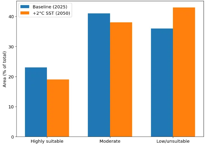
Figure 8. Projected climate-change sensitivity of Pinctada radiata habitats under a +2 °C SST scenario (2050). Orange colors indicate a loss of suitability relative to baseline conditions, while blue tones indicate areas where suitability persists or increases. Predictions are derived from the +2 °C ensemble simulation at 100 m resolution.
4. Discussion
The results of this study indicate that the distribution of P. radiata in the Maliakos and South Evoikos Gulfs is mainly governed by temperature, oxygen availability, and substrate type. Using Copernicus-derived climatologies, the ensemble consistently identified an optimum suitability range of roughly 20–26 °C and dissolved-oxygen concentrations above 6 mg·L−1. These values broadly agree with previously reported physiological tolerances for the species, which suggest thermal sensitivity beyond ~27–28 °C and reduced aerobic performance under low-oxygen conditions [114,115,116]. It should be emphasized, however, that these values represent probabilistic optima based on long-term climatologies; short-lived heat pulses or episodic hypoxia, which are not fully resolved by decadal averages, may impose additional constraints in situ.
Contrasts between the two gulfs underscore the strong role of watershed–coastal interactions in semi-enclosed Mediterranean systems. The Maliakos Gulf, which receives continuous freshwater input from the Spercheios River, displays pronounced gradients in salinity, nutrients, and oxygen. These conditions create mesotrophic, low-energy environments that often favor P. radiata, yet they also expose the gulf to seasonal stratification and temporary hypoxic episodes patterns well documented in shallow embayments of the Aegean [117,118]. By contrast, the more open South Evoikos Gulf benefits from regular exchange with the Aegean through the Cavo Doro Strait. This enhances bottom-water ventilation and sustains relatively stable hydrographic conditions, features that can increase resilience to warming and oxygen stress. Similar patterns have been reported in other well-flushed eastern Mediterranean basins [119].
The integration of a convolutional neural network with more established approaches, such as MaxEnt and XGBoost, proved useful for capturing spatial structure and improved the overall interpretability of the modelling system. Although the gain in predictive performance from the CNN alone was modest, its spatial outputs were more coherent, and the use of Grad-CAM provided clear visual insight into the spatial features guiding predictions. When combined with SHAP-based analyses, the interpretability framework revealed consistent interactions between temperature and oxygen interactions that align well with known physiological constraints of Mediterranean bivalves. This emphasis on explainability reflects broader shifts in marine ecological modelling towards transparent and interpretable machine-learning practices [120,121].
The +2 °C SST warming scenario highlighted the relative vulnerability of shallow and stratified systems such as Maliakos, where high-suitability habitat contracted by approximately 18–22%. This pattern mirrors basin-wide projections of intensified summer warming and declining oxygen in semi-enclosed Mediterranean gulfs [122,123]. In contrast, some areas of the South Evoikos Gulf showed localized increases in moderate suitability, likely reflecting its stronger hydrodynamic connection to the open Aegean, which can buffer warming impacts through enhanced mixing. These findings support emerging evidence that fine-scale hydrodynamic variation can modulate climate sensitivity at regional scales in the eastern Mediterranean [124].
From a management perspective, the identification of high-suitability areas near the Spercheios delta offers valuable guidance for monitoring, conservation planning, and potential aquaculture siting. However, these areas are also susceptible to eutrophication and episodic hypoxia, indicating that suitability assessments should be paired with environmental risk evaluations. The results complement priorities under the Marine Strategy Framework Directive and support the goals of the EU Biodiversity Strategy 2030 by providing spatially explicit indicators of habitat condition and climate sensitivity. Furthermore, the use of open-access Copernicus data and transparent analytical workflows aligns with the objectives of the European Digital Twin Ocean initiative [125].
Despite the strengths of the modelling framework, several limitations should be acknowledged. The reliance on presence-only observations means that some degree of sampling bias may remain, even after applying KDE-based corrections. In addition, the use of long-term climatological averages inevitably smooths short-lived extremes, such as brief hypoxic episodes or rapid nutrient pulses, which may be ecologically important in shallow systems. Although the CNN combined with Grad-CAM offered valuable spatial insight, parts of the internal feature-extraction process are still difficult to interpret mechanistically in an ecological context. Future work could benefit from integrating time-resolved Copernicus products, continuous in situ sensor records, and coupled hydrodynamic–biogeochemical models to improve the temporal fidelity of predictions. Including biotic interactions such as competition or predation may also enhance ecological realism, while extending the framework to multi-species models could help illuminate broader community-level responses to environmental gradients.
Overall, this study demonstrates how Copernicus Earth Observation datasets, ensemble machine learning methods, and explainable AI tools can be combined to produce a transparent and robust representation of benthic habitat patterns. By linking watershed influences, hydrographic variability, and habitat suitability within a single framework, the study contributes to the development of integrated coastal-ecosystem assessments and provides a scalable approach to support adaptive management in the face of ongoing environmental change.
5. Conclusions
This study shows that combining Copernicus Earth Observation products with modern machine-learning and deep-learning techniques provides a strong basis for assessing the habitat suitability of P. radiata in two semi-enclosed systems of Central Greece that differ markedly in their environmental characteristics. By integrating long-term physical and biogeochemical climatologies within an ensemble modelling framework, we were able to capture the main environmental gradients that structure benthic habitats in transitional Mediterranean environments [126].
The ensemble comprising MaxEnt, XGBoost, and a CNN performed well across spatially independent folds and consistently identified sea-surface temperature, dissolved oxygen, and substrate as the primary drivers shaping the species’ distribution. These results are consistent with known physiological responses of P. radiata, particularly its sensitivity to the combined effects of warming and reduced oxygen in stratified basins [127]. The use of explainable-AI methods (SHAP and Grad-CAM) added interpretive value by linking model behavior to ecologically meaningful mechanisms, thereby improving the transparency and credibility of the predictions.
Spatial predictions indicated that roughly two-thirds of the study area exhibits moderate to high suitability, with optimal habitats concentrated in shallow, low-energy settings, most notably in the central Maliakos basin and along sheltered coastal shelves in the South Evoikos Gulf. Under a +2 °C SST warming scenario, high-suitability areas decreased by 18–22%, particularly in thermally sensitive and nutrient-influenced parts of Maliakos. These shifts mirror regional projections of habitat compression and decreasing oxygen availability in semi-enclosed Mediterranean gulfs under continued warming [128,129].
The methodological framework aligns well with the goals of the EU Marine Strategy Framework Directive and the EU Biodiversity Strategy 2030 by offering a transparent, reproducible, and operational pathway for integrating EO data into marine spatial planning and ecosystem-based management. Its adherence to FAIR principles and compatibility with containerized, open-access workflows also support the broader development of European Digital Twin Ocean initiatives [130,131].
In summary, this work contributes to the advance of integrated coastal-ecosystem assessment by linking watershed inputs, hydrographic variability, and benthic habitat dynamics within a unified analytical approach. As climatic and human-induced pressures continue to intensify, transparent and data-driven modelling frameworks such as the one presented here will become increasingly important for anticipating ecological change, guiding adaptive management and supporting the sustainable stewardship of Mediterranean coastal systems.
Statement of the Use of Generative AI and AI-Assisted Technologies in the Writing Process
During the preparation of this manuscript, the authors used ChatGPT (OpenAI) in order to improve English language, grammar, and readability. After using this tool, the authors reviewed and edited the content as needed and take full responsibility for the content of the published article.
Acknowledgments
This research was supported by the research program of the Region of Central Greece (Project Code: Π89-2.13), implemented under the “Regional Development Programme (PPA) of Central Greece”, Priority Axis 2.4 “Risk Prevention and Management”, entitled “Investigation of the Biology, Fisheries, Ecology, and Population Dynamics of the bivalve pearl oyster Pinctada imbricata radiata in the South Evoikos and Maliakos Gulfs”.
Author Contributions
Conceptualization, D.P. and D.K.; Methodology, D.P.; Software, D.P.; Validation, D.P., D.K., A.C., D.V. and G.K.; Formal Analysis, D.P.; Investigation, D.P.; Resources, D.K., A.C., D.V. and G.K.; Data Curation, D.P.; Writing-Original Draft Preparation, D.P.; Writing-Review & Editing, D.P., D.K., A.C., D.V. and G.K.; Visualization, D.P.; Supervision, D.K.; Project Administration, D.K.; Funding Acquisition, D.K. All authors have read and agreed to the published version of the manuscript.
Ethics Statement
Not applicable.
Informed Consent Statement
Not applicable.
Data Availability Statement
The data supporting the findings of this study are available from the corresponding author upon reasonable request. Environmental datasets used in this study were obtained from publicly accessible repositories, including the Copernicus Marine Environment Monitoring Service (CMEMS) and EMODnet. Processed datasets and model outputs generated during the study are available from the corresponding author upon reasonable request.
Funding
This research was funded by the Region of Central Greece, under the Regional Development Programme (PPA), Priority Axis 2.4 “Risk Prevention and Management”, Project Code: Π89-2.13.
Declaration of Competing Interest
The authors declare that they have no known competing financial interests or personal relationships that could have appeared to influence the work reported in this paper.
References
- Coll M, Piroddi C, Steenbeek J, Kaschner K, Ben Rais Lasram F, Aguzzi J, et al. The biodiversity of the Mediterranean Sea: Estimates, patterns, and threats. PLoS ONE 2010, 5, e11842. DOI:10.1371/journal.pone.0011842 [Google Scholar]
- Bianchi CN, Morri C. Marine biodiversity of the Mediterranean Sea: Situation, problems and prospects for future research. Mar. Pollut. Bull. 2000, 40, 367–376. DOI:10.1016/S0025-326X(00)00027-8 [Google Scholar]
- UNEP/MAP. Mediterranean Quality Status Report 2017; United Nations Environment Programme: Athens, Greece, 2017. [Google Scholar]
- Cloern JE. Our evolving conceptual model of the coastal eutrophication problem. Mar. Ecol. Prog. Ser. 2001, 210, 223–253. DOI:10.3354/meps210223 [Google Scholar]
- Diaz RJ, Rosenberg R. Spreading dead zones and consequences for marine ecosystems. Science 2008, 321, 926–929. DOI:10.1126/science.1156401 [Google Scholar]
- Solidoro C, Bastianini M, Bandelj V, Codermatz R, Cossarini G, Melaku Canu D, et al. Current state, scales of variability and trends of biogeochemical properties in the Northern Adriatic Sea. J. Geophys. Res. Ocean. 2009, 114, C07S91. DOI:10.1029/2008jc004838 [Google Scholar]
- Pörtner HO, Bock C, Mark FC. Oxygen- and capacity-limited thermal tolerance: Bridging ecology and physiology. J. Exp. Biol. 2017, 220, 2685–2696. DOI:10.1242/jeb.134585 [Google Scholar]
- Kassis D, Krasakopoulou E, Korres G, Petihakis G, Triantafyllou GS. Hydrodynamic features of the South Aegean Sea as derived from Argo T/S and dissolved oxygen profiles in the area. Ocean Dynamics 2016, 66, 1449–1466. DOI:10.1007/s10236-016-0987-2 [Google Scholar]
- Simboura N, Tsapakis M, Pavlidou A, Assimakopoulou G, Pagou K, Kontoyannis H, et al. Assessment of the environmental status in Hellenic coastal waters (Eastern Mediterranean): From the Water Framework Directive to the Marine Strategy Water Framework Directive. Mediterr. Mar. Sci. 2015, 16, 46–64. DOI:10.12681/mms.960 [Google Scholar]
- Poulos SE, Collins MB, Pattiaratchi C, Cramp A, Gull W, Tsimplis M, et al. Oceanography and sedimentation in the semi-enclosed, deep-water Gulf of Corinth (Greece). Mar. Geol. 1996, 134, 213–235. DOI:10.1016/0025-3227(96)00028-X [Google Scholar]
- Zenetos A, Gofas S, Verlaque M, Çinar ME, García Raso JE, Bianchi CN, et al. Alien species in the Mediterranean Sea by 2010. A contribution to the application of European Union’s Marine Strategy Framework Directive (MSFD). Part 2. Introduction trends and pathways. Mediterr. Mar. Sci. 2012, 13, 328–352. DOI:10.12681/mms.327 [Google Scholar]
- Giovos I, Kleitou P, Poursanidis D, Batjakas I, Bernardi G, Crocetta F, et al. Citizen-science for monitoring marine invasions and stimulating public engagement: A case project from the eastern Mediterranean. Biol. Invasions 2019, 21, 3707–3721. DOI:10.1007/s10530-019-02083-w [Google Scholar]
- Claudet J, Fraschetti S. Human-driven impacts on marine habitats: A regional meta-analysis in the Mediterranean Sea. Biol. Conserv. 2010, 143, 2195–2206. DOI:10.1016/j.biocon.2010.06.004 [Google Scholar]
- Oral M. Alien fish species in the Mediterranean–Black Sea basin. J. Black Sea/Mediterr. Environ. 2010, 16, 87–132. Available online: https://blackmeditjournal.org/wp-content/uploads/87-132.pdf (accessed on 7 March 2026).
- Tlig-Zouari S, Rabaoui L, Irathni I, Ben Hassine OK. Distribution, habitat and population densities of the invasive species Pinctada radiata (Molluca: Bivalvia) along the Northern and Eastern coasts of Tunisia. Cah. De Biol. Mar. 2009, 50, 131–142. [Google Scholar]
- Pafras D, Theocharis A, Kondylatos G, Conides A, Klaoudatos D. Population Biology of the Non-Indigenous Rayed Pearl Oyster (Pinctada radiata) in the South Evoikos Gulf, Greece. Diversity. 2024, 16, 460. DOI:10.3390/d16080460 [Google Scholar]
- Hoang TH, Stone DA, Duong DN, Bansemer MS, Harris JO, Qin JG. Colour change of greenlip abalone (Haliotis laevigata Donovan) fed formulated diets containing graded levels of dried macroalgae meal. Aquaculture 2017, 468, 278–285. DOI:10.1016/j.aquaculture.2016.10.027 [Google Scholar]
- Valero Rodriguez JM, Aguilar J, Fernandez-Gonzalez V. Species Selection of Macroalgae with Potential Bioactive Metabolites for Novel Design of IMTA in Offshore Coast Areas of the Mediterranean Sea. Available online: https://ssrn.com/abstract=5745349 (accessed on 7 March 2026).
- Gavrilović A, Piria M, Guo XZ, Jug-Dujaković J, Ljubučić A, Krkić A, et al. First evidence of establishment of the rayed pearl oyster, Pinctada imbricata radiata (Leach, 1814), in the eastern Adriatic Sea. Mar. Pollut. Bull. 2017, 125, 556–560. DOI:10.1016/j.marpolbul.2017.10.045 [Google Scholar]
- Derbali A, Jarboui O, Ghorbel M. Distribution, Abundance and Population Structure of Pinctada radiata (Mollusca: Bivalvia) in Southern Tunisian Waters (Central Mediterranean). 2011. Available online: https://www.cabidigitallibrary.org/doi/full/10.5555/20113062770 (accessed on 7 March 2026).
- Lassoued M, Smaoui-Damak W, Hamza-Chaffai A. Reproductive cycle of the pearl oyster, Pinctada radiata (Mollusca: Pteridae), in the Zarat site (Gulf of Gabès, Tunisia). Euro-Mediterr. J. Environ. Integr. 2018, 3, 18. DOI:10.1007/s41207-018-0056-y [Google Scholar]
- Aguilo-Arce J, Ferragut JF, Png-Gonzalez L, Carbonell A, Capa M. First genetic survey on the invasive rayed pearl oyster Pinctada radiata (Leach, 1814) populations of the Balearic Islands (Western Mediterranean). Mediterr. Mar. Sci. 2023, 24, 666–678. DOI:10.12681/mms.34195 [Google Scholar]
- Theodorou JA, Perdikaris C, Spinos E. On the occurrence of rayed pearl oyster Pinctada imbricata radiata (Leach, 1814) in Western Greece (Ionian Sea) and its biofouling potential. Biharean Biol. 2019, 13, 4–7. Available online: https://www.researchgate.net/profile/Costas-Perdikaris/publication/327401904_On_the_occurrence_of_rayed_pearl_oyster_Pinctada_imbricata_radiata_Leach_1814_in_Western_Greece_Ionian_Sea_and_its_biofouling_potential/links/5d10545f92851cf4404646c2/On-the-occurrence-of-rayed-pearl-oyster-Pinctada-imbricata-radiata-Leach-1814-in-Western-Greece-Ionian-Sea-and-its-biofouling-potential.pdf (accessed on 7 March 2026).
- Zenetos A, Pancucci-Papadopoulou M, Zogaris S, Papastergiadou E, Vardakas L, Aligizaki K, et al. Aquatic alien species in Greece (2009): Tracking sources, patterns and effects on the ecosystem. J. Biol. Research. Sci. Ann. Sch. Biol. 2009, 12, 135–172. Available online: https://www.academia.edu/download/39261062/0046352ac476cec891000000.pdf (accessed on 7 March 2026).
- Wada KT, Temkin I. Taxonomy and phylogeny of pearl oysters. In The Pearl Oyster, 2nd ed.; Southgate PC, Lucas JS, Eds.; Elsevier: Amsterdam, The Netherlands, 2008; pp. 37–75. [Google Scholar]
- Southgate PC, Militz TA. Nutrient Compositions of Adductor Muscle from the Pearl Oysters Pinctada maxima and Pinctada margaritifera. J. Shellfish. Res. 2023, 42, 465–469. DOI:10.2983/035.042.0309 [Google Scholar]
- Galanidi M, Zenetos A, Bacher S. Assessing the socio-economic impacts of priority marine invasive fishes in the Mediterranean with the newly proposed SEICAT methodology. Mediterr. Mar. Sci. 2018, 19, 107. DOI:10.12681/mms.15940 [Google Scholar]
- Al Saadi A. Population Structure and Patterns of Genetic Variation in a Pearl Oyster (Pinctada radiata) Native to the Arabian Gulf. Ph.D. Dissertation, Queensland University of Technology, Brisbane, Australia, 2013. [Google Scholar]
- Pafras D, Apostologamvrou C, Balatsou A, Theocharis A, Lolas A, Hatziioannou M, et al. Reproductive Biology of Pearl Oyster (Pinctada radiata, Leach 1814) Based on Microscopic and Macroscopic Assessment of Both Sexes in the Eastern Mediterranean (South Evia Island). J. Mar. Sci. Eng. 2024, 12, 1259. DOI:10.3390/jmse12081259 [Google Scholar]
- Brando VE, Santoleri R, Colella S, Volpe G, Di Cicco A, Sammartino M, et al. Overview of operational global and regional Ocean Colour essential ocean variables within the Copernicus marine Service. Remote Sens. 2024, 16, 4588. DOI:10.3390/rs16234588 [Google Scholar]
- Wolters E, Toté C, Sterckx S, Adriaensen S, Henocq C, Bruniquel J, et al. iCOR Atmospheric correction on Sentinel-3/OLCI over land: Intercomparison with AERONET, RadCalNet, and SYN Level-2. Remote Sens. 2021, 13, 654. DOI:10.3390/rs13040654 [Google Scholar]
- Kerr JT, Ostrovsky M. From space to species: Ecological applications for remote sensing. Trends Ecol. Evol. 2003, 18, 299–305. DOI:10.1016/S0169-5347(03)00071-5 [Google Scholar]
- Fingas M. Remote Sensing for Marine Management. In World Seas: An Environmental Evaluation, 2nd ed.; Sheppard C, Ed.; Elsevier: Amsterdam, The Netherlands; Academic Press: Cambridge, MA, USA, 2019; pp. 103–119. DOI:10.1016/B978-0-12-805052-1.00005-X [Google Scholar]
- Elith J, Leathwick JR. Species Distribution Models: Ecological Explanation and Prediction Across Space and Time. Annu. Rev. Ecol. Evol. Syst. 2009, 40, 677–697. DOI:10.1146/annurev.ecolsys.110308.120159 [Google Scholar]
- Guisan A, Zimmermann NE. Predictive habitat distribution models in ecology. Ecol. Modell. 2000, 135, 147–186. DOI:10.1016/S0304-3800(00)00354-9 [Google Scholar]
- Phillips SJ, Anderson RP, Schapire RE. Maximum entropy modeling of species geographic distributions. Ecol. Modell. 2006, 190, 231–259. DOI:10.1016/j.ecolmodel.2005.03.026 [Google Scholar]
- Franklin J. Mapping Species Distributions: Spatial Inference and Prediction; Cambridge University Press: Cambridge, UK, 2010. DOI:10.1017/S0030605310001201 [Google Scholar]
- Melo-Merino SM, Reyes-Bonilla H, Lira-Noriega A. Ecological niche models and species distribution models in marine environments: A literature review and spatial analysis of evidence. Ecol. Modell. 2020, 415, 108837. DOI:10.1016/j.ecolmodel.2019.108837 [Google Scholar]
- Olden JD, Lawler JJ, Poff NL. Machine learning methods without tears: A primer for ecologists. Q. Rev. Biol. 2008, 83, 171–193. DOI:10.1086/587826 [Google Scholar]
- Breiman L. Random forests. Mach. Learn. 2001, 45, 5–32. DOI:10.1023/A:1010933404324 [Google Scholar]
- Friedman JH. Greedy function approximation: A gradient boosting machine. Ann. Stat. 2001, 29, 1189–1232. DOI:10.1214/aos/1013203451 [Google Scholar]
- Chen T, Guestrin C. XGBoost: A scalable tree boosting system. In Proceedings of the 22nd ACM SIGKDD International Conference on Knowledge Discovery and Data Mining, San Francisco, CA, USA, 13–17 August 2016; pp. 785–794. DOI:10.1145/2939672.2939785 [Google Scholar]
- Hinton GE. Learning multiple layers of representation. Trends Cogn. Sci. 2007, 11, 428–434. DOI:10.1016/j.tics.2007.09.004 [Google Scholar]
- Lundberg SM, Lee S-I. A unified approach to interpreting model predictions. In Advances in Neural Information Processing Systems (NIPS); NeurIPS Proceedings: San Diego, CA, USA, 2017; pp. 4765–4774. [Google Scholar]
- Selvaraju RR, Cogswell M, Das A, Vedantam R, Parikh D, Batra D. Grad-CAM: Visual explanations from deep networks. In Proceedings of the 2017 IEEE International Conference on Computer Vision (ICCV), Venice, Italy, 22–29 October 2017; pp. 618–626. DOI:10.1109/ICCV.2017.74 [Google Scholar]
- Hengl T, Nussbaum M, Wright MN, Heuvelink GB, Gräler B. Random forest as a generic framework for predictive modeling of spatial and spatio-temporal variables. PeerJ 2018, 6, e5518. DOI:10.7717/peerj.5518 [Google Scholar]
- Leroy B. Choosing presence-only species distribution models. J. Biogeogr. 2022, 50, 247–250. DOI:10.1111/jbi.14505 [Google Scholar]
- Souissi S, Molinero JC, Beaugrand G, Anneville O, Licandro P, Schmitt F, et al. Effects of global changes on aquatic ecosystems in Western Europe: Role of plankton communities. GLOBEC Int. Newsl. 2007, 13, 23–25. Available online: https://oceanrep.geomar.de/id/eprint/3300/1/GLOBEC_13_1_part1.pdf (accessed on 7 March 2026).
- Stathopoulos N, Kalogeropoulos K, Vasileiou E, Louka P, Tsesmelis DE, Tsatsaris A. Charting the changes: Geographic Information System and Remote Sensing study on soil erosion and coastal transformations in Maliakos Gulf, Greece. In Geographical Information Science; Elsevier: Amsterdam, The Netherlands, 2024; pp. 207–230. DOI:10.1016/B978-0-443-13605-4.00005-9 [Google Scholar]
- Tintoré J, Pinardi N, Álvarez-Fanjul E, Aguiar E, Álvarez-Berastegui D, Bajo M, et al. Challenges for sustained observing and forecasting systems in the Mediterranean Sea. Front. Mar. Sci. 2019, 6, 568. DOI:10.3389/fmars.2019.00568 [Google Scholar]
- Katsanevakis S, Tempera F, Teixeira H. Mapping the impact of alien species on marine ecosystems: The Mediterranean Sea case study. Divers. Distrib. 2016, 22, 694–707. DOI:10.1111/ddi.12429 [Google Scholar]
- Beaugrand G, Kirby RR. Quasi-deterministic responses of marine species to climate change. Clim. Res. 2016, 69, 117–128. DOI:10.3354/cr01398 [Google Scholar]
- Aspioti AG, Fourniotis NT. A brief review of hydrodynamic circulation in the Mediterranean gulfs. Dynamics 2024, 4, 873–888. DOI:10.3390/dynamics4040045 [Google Scholar]
- Zananiri I, Vakalas I. Surficial Sediment Distribution in a Complex Marine Setting The Example of Coastal and Open Sea Areas of Evia Island, Central Aegean, Greece. Oceans 2025, 6, 8. DOI:10.3390/oceans6010008 [Google Scholar]
- ΠΟΥΛΟΣ ΣE, ΔΡΑΚΟΠΟΥΛΟΣ ΠΓ, ΛΕΟΝΤΑΡΗΣ ΣΝ, ΤΣΑΠΑΚΗΣ Ε, ΧΑΤΖΗΓΙΑΝΝΗ Ε. The Contribution of Tidal Currents to the Sedimentation of the Strait of Avlida, Southern Evoikos Gulf (Greece). Bull. Geol. Soc. Greece 2018, 34, 731–736. DOI:10.12681/bgsg.17350 [Google Scholar]
- Dimitriou PD, Karakassis I, Pitta P, Tsagaraki TM, Apostolaki ET, Magiopoulos I, et al. Mussel farming in Maliakos Gulf and quality indicators of the marine environment: Good benthic below poor pelagic ecological status. Mar. Pollut. Bull. 2015, 101, 784–793. DOI:10.1016/j.marpolbul.2015.09.035 [Google Scholar]
- Araújo MB, Peterson AT. Uses and misuses of bioclimatic envelope modeling. Ecology 2012, 93, 1527–1539. DOI:10.1890/11-1930.1 [Google Scholar]
- Beck HE, Zimmermann NE, McVicar TR, Vergopolan N, Berg A, Wood EF. Present and future Köppen-Geiger climate classification maps at 1-km resolution. Sci. Data. 2018, 5, 180214. DOI:10.1038/sdata.2018.214 [Google Scholar]
- Kuhn M, Johnson K. Applied Predictive Modeling; Springer: New York, NY, USA, 2013; Volume 26, p. 13. [Google Scholar]
- Motrenko A, Strijov V. Multi-way feature selection for ECoG-based Brain-Computer Interface. Expert Syst. Appl. 2018, 114, 402–413. DOI:10.1016/j.eswa.2018.06.054 [Google Scholar]
- Soininen J, Luoto M. Predictability in species distributions: A global analysis across organisms and ecosystems. Glob. Ecol. Biogeogr. 2014, 23, 1264–1274. DOI:10.1111/geb.12204 [Google Scholar]
- Czarnoleski M, Kozlowski J, Lewandowski K, Müller T, Stanczykowska A. The Zebra Mussel in Europe; Backhuys Publishers: Leiden, The Netherlands; Margraf Publishers: Weikersheim, Germany, 2010. [Google Scholar]
- Lejeusne C, Chevaldonné P, Pergent-Martini C, Boudouresque CF, Pérez T. Climate change effects on a miniature ocean: The highly diverse, highly impacted Mediterranean Sea. Trends Ecol. Evol. 2010, 25, 250–260. DOI:10.1016/j.tree.2009.10.009 [Google Scholar]
- Vaquer-Sunyer R, Duarte CM. Thresholds of hypoxia for marine biodiversity. Proc. Natl. Acad. Sci. USA 2008, 105, 15452–15457. DOI:10.1073/pnas.0803833105 [Google Scholar]
- Behrenfeld MJ, Boss ES. Resurrecting the ecological underpinnings of ocean plankton blooms. Annu. Rev. Mar. Sci. 2014, 6, 167–194. DOI:10.1146/annurev-marine-052913-021325 [Google Scholar]
- Scheuring CI. Impact of Ocean Acidification (OA) on the Acid-Base Regulation of Polar Cod: Time and Localized Tracking of Brain pH Changes. Ph.D. Dissertation, Universität Rostock, Rostock, Germany, 2019. [Google Scholar]
- Treml EA, Halpin PN, Urban DL, Pratson LF. Modeling population connectivity by ocean currents, a graph-theoretic approach for marine conservation. Landsc. Ecol. 2008, 23 (Suppl. S1), 19–36. DOI:10.1007/s10980-007-9138-y [Google Scholar]
- Speight MR, Henderson PA. Marine Ecology: Concepts and Applications; John Wiley & Sons: Hoboken, NJ, USA, 2013. [Google Scholar]
- Lucena-Moya P, Gómez-Rodríguez C, Pardo I. Spatio-temporal variability in water chemistry of Mediterranean coastal lagoons and its management implications. Wetlands 2012, 32, 1033–1045. DOI:10.1007/s13157-012-0334-4 [Google Scholar]
- Powley HR, Van Cappellen P, Krom MD. Nutrient cycling in the Mediterranean Sea: The key to understanding how the unique marine ecosystem functions and responds to anthropogenic pressures. In Mediterranean Identities-Environment, Society, Culture; InTech: London, UK, 2017; pp. 47–77. DOI:10.5772/intechopen.70878 [Google Scholar]
- Stolar J, Nielsen SE, Franklin J. Accounting for spatially biased sampling effort in presence-only species distribution modelling. Divers. Distrib. 2015, 21, 595–608. DOI:10.1111/ddi.12279 [Google Scholar]
- Pebesma E. Simple Features for R: Standardized Support for Spatial Vector Data. R J. 2018, 10, 439. DOI:10.32614/RJ-2018-009 [Google Scholar]
- Katsanevakis S, Wallentinus I, Zenetos A, Leppäkoski E, Çinar ME, Ozturk B, et al. Impacts of invasive alien marine species on ecosystem services and biodiversity: A pan-European review. Aquat. Invasions 2014, 9, 391–423. DOI:10.3391/ai.2014.9.4.01 [Google Scholar]
- Occhipinti-Ambrogi A, Marchini A, Cantone G, Castelli A, Chimenz C, Cormaci M, et al. Alien species along the Italian coasts: An overview. Biol. Invasions 2011, 13, 215–237. DOI:10.1007/s10530-010-9803-y [Google Scholar]
- Rotter A, Klun K, Francé J, Mozetič P, Orlando-Bonaca M. Non-indigenous species in the Mediterranean Sea: Turning from pest to source by developing the 8Rs model, a new paradigm in pollution mitigation. Front. Mar. Sci. 2020, 7, 178. DOI:10.3389/fmars.2020.00178 [Google Scholar]
- Silverman BW. Density Estimation for Statistics and Data Analysis; Routledge: London, UK, 2018. DOI:10.1201/9781315140919 [Google Scholar]
- Phillips SJ, Dudík M, Elith J, Graham CH, Lehmann A, Leathwick J, et al. Sample selection bias and presence-only distribution models: Implications for background and pseudo-absence data. Ecol. Appl. 2009, 19, 181–197. DOI:10.1890/07-2153.1 [Google Scholar]
- Dormann CF, Elith J, Bacher S, Buchmann C, Carl G, Carré G, et al. Collinearity: A review of methods to deal with it and a simulation study evaluating their performance. Ecography 2013, 36, 27–46. DOI:10.1111/j.1600-0587.2012.07348.x [Google Scholar]
- Zuur AF, Ieno EN, Elphick CS. A protocol for data exploration to avoid common statistical problems. Methods Ecol. Evol. 2010, 1, 3–14. DOI:10.1111/j.2041-210X.2009.00001.x [Google Scholar]
- Guisan A, Thuiller W, Zimmermann NE. Habitat Suitability and Distribution Models: With Applications in R; Cambridge University Press: Cambridge, UK, 2017. [Google Scholar]
- Breiner FT, Guisan A, Bergamini A, Nobis MP. Overcoming limitations of modelling rare species by using ensembles of small models. Methods Ecol. Evol. 2015, 6, 1210–1218. DOI:10.1111/2041-210X.12403 [Google Scholar]
- Bivand RS, Pebesma E, Gómez-Rubio V. Applied Spatial Data Analysis with R, 2nd ed.; Springer: Berlin/Heidelberg, Germany, 2013. DOI:10.1007/978-0-387-78171-6_8 [Google Scholar]
- Legendre P, Legendre L. Numerical Ecology, 3rd ed.; Elsevier: Amsterdam, The Netherlands, 2012. [Google Scholar]
- Araújo MB, New M. Ensemble forecasting of species distributions. Trends Ecol. Evol. 2007, 22, 42–47. DOI:10.1016/j.tree.2006.09.010 [Google Scholar]
- Thuiller W, Lafourcade B, Engler R, Araújo MB. BIOMOD—A platform for ensemble forecasting of species distributions. Ecography 2009, 32, 369–373. DOI:10.1111/j.1600-0587.2008.05742.x [Google Scholar]
- Schneider F. Adaptation of Baccharis L. in Chile to environmental factors on a landscape scale. In Evolution in the Genus Baccharis L.; Verlagsname nicht ermittelbar: Dresden, Germany, 2025; p. 137. [Google Scholar]
- Phillips SJ, Dudík M. Modeling of species distributions with Maxent: New extensions and a comprehensive evaluation. Ecography 2008, 31, 161–175. DOI:10.1111/j.0906-7590.2008.5203.x [Google Scholar]
- Temlyakov V. Sparse sampling recovery by greedy algorithms. IMA J. Numer. Anal. 2025, 45, draf054. DOI:10.1093/imanum/draf054 [Google Scholar]
- Lecun Y, Bengio Y, Hinton G. Deep learning. Nature 2015, 521, 436–444. DOI:10.1038/nature14539 [Google Scholar]
- Vamosi SM, Heard SB, Vamosi JC, Webb CO. Emerging patterns in the comparative analysis of phylogenetic community structure. Mol. Ecol. 2009, 18, 572–592. DOI:10.1111/j.1365-294X.2008.04001.x [Google Scholar]
- Marmion M, Parviainen M, Luoto M, Heikkinen RK, Thuiller W. Evaluation of consensus methods in predictive species distribution modelling. Divers. Distrib. 2009, 15, 59–69. DOI:10.1111/j.1472-4642.2008.00491.x [Google Scholar]
- Hao T, Elith J, Guillera-Arroita G, Lahoz-Monfort JJ, Serra‐Diaz J. A review of evidence about use and performance of species distribution modelling ensembles like BIOMOD. Divers. Distrib. 2019, 25, 839-852. DOI:10.1111/ddi.12892 [Google Scholar]
- Valavi R, Elith J, Lahoz-Monfort JJ, Guillera-Arroita G. blockCV: An R package for generating spatially or environmentally separated folds for k-fold cross-validation of species distribution models. Methods Ecol. Evol. 2019, 10, 225–232. DOI:10.1101/357798 [Google Scholar]
- Demler OV, Pencina MJ, D’Agostino RB, Sr. Misuse of the DeLong test to compare AUCs for nested models. Stat. Methods Med. Res. 2012, 21, 361–373. DOI:10.1002/sim.5328 [Google Scholar]
- Peterson AT, Papes M, Soberón J. Rethinking receiver operating characteristic analysis: Ecological niche modeling evaluation. Ecol. Model. 2008, 213, 63–72. DOI:10.1016/j.ecolmodel.2007.11.008 [Google Scholar]
- Molnar C. Interpretable Machine Learning, 2nd ed.; Lulu.com: Morrisville, NC, USA, 2022. [Google Scholar]
- Zimmer AC. A model for the interpretation of verbal predictions. Int. J. Man-Mach. Stud. 1984, 20, 121–134. DOI:10.1016/S0020-7373(84)80009-7 [Google Scholar]
- Debray TP, Damen JA, Snell KI, Ensor J, Hooft L, Reitsma JB, et al. A guide to systematic review and meta-analysis of prediction model performance. BMJ 2017, 356, i6460. DOI:10.1136/bmj.i6460 [Google Scholar]
- Ribeiro MT, Singh S, Guestrin C. “Why Should I Trust You?” Explaining the predictions of any classifier. In Proceedings of the 22nd ACM SIGKDD International Conference on Knowledge Discovery and Data Mining, San Francisco, CA, USA, 13–17 August 2016; pp. 1135–1144. DOI:10.1145/2939672.2939778 [Google Scholar]
- Zhao F, Luo H, Geng H, Sun Q. An RSSI gradient-based AP localization algorithm. China Commun. 2014, 11, 100–108. DOI:10.1109/CC.2014.6821742 [Google Scholar]
- Johnson LB. Analyzing spatial and temporal phenomena using geographical information systems: A review of ecological applications. Landsc. Ecol. 1990, 4, 31–43. DOI:10.1007/BF02573949 [Google Scholar]
- Elith J, Kearney M, Phillips SJ. The art of modelling range-shifting species. Methods Ecol. Evol. 2010, 1, 330–342. DOI:10.1111/j.2041-210X.2010.00036.x [Google Scholar]
- Biecek P. Explanatory Model Analysis; Chapman & Hall/CRC Press: Boca Raton, FL, USA, 2021. DOI:10.1201/9780429027192 [Google Scholar]
- Murphy K. Probabilistic Machine Learning: Advanced Topics; MIT Press: Cambridge, MA, USA, 2023. [Google Scholar]
- Liu C, White M, Newell G, Pearson R. Selecting thresholds for the prediction of species occurrence with presence-only data. J. Biogeogr. 2013, 40, 778–789. DOI:10.1111/jbi.12058 [Google Scholar]
- Roberts DR, Bahn V, Ciuti S, Boyce MS, Elith J, Guillera‐Arroita G, et al. Cross-validation strategies for data with temporal, spatial, hierarchical, or phylogenetic structure. Ecography 2017, 40, 913–929. DOI:10.1111/ecog.02881 [Google Scholar]
- Beale CM, Lennon JJ, Gimona A. Opening the climate envelope reveals no macroscale associations with climate in European birds. Proc. Natl. Acad. Sci. USA 2008, 105, 14908–14912. DOI:10.1073/pnas.0803506105 [Google Scholar]
- Forrestal FC, Schirripa M, Goodyear CP, Arrizabalaga H, Babcock EA, Coelho R, et al. Testing robustness of CPUE standardization and inclusion of environmental variables with simulated longline catch datasets. Fish. Res. 2019, 210, 1–13. DOI:10.1016/j.fishres.2018.09.025 [Google Scholar]
- Maréchaux I, Fischer FJ, Schmitt S, Chave J. TROLL 4.0: Representing water and carbon fluxes, leaf phenology and intraspecific trait variation in a mixed-species individual-based forest dynamics model–Part 1: Model description. Geosci. Model Dev. 2025, 18, 5143–5204. DOI:10.5194/gmd-18-5143-2025 [Google Scholar]
- Anselin L. An Introduction to Spatial Autocorrelation Analysis with GeoDa; Spatial Analysis Laboratory, University of Illinois, Champagne-Urbana: Champaign, IL, USA, 2003. [Google Scholar]
- Thuiller W, Münkemüller T. Habitat suitability modeling. In Effects of Climate Change on Birds; Oxford University Press: Oxford, UK, 2010; pp. 77–85. [Google Scholar]
- Hijmans RJ, Elith J. Species Distribution Modeling with R. R Cran Project. 2013. Available online: https://www.researchgate.net/profile/Mohamed-Mourad-Lafifi/post/How_to_loop_multiple_maxent_models/attachment/5f4c3571ce377e00016fe61a/AS%3A930374343483392%401598829937118/download/Species+distribution+modeling+with+R.pdf (accessed on 7 March 2026).
- Zurell D, Franklin J, König C, Bouchet PJ, Dormann CF, Elith J, et al. A standard protocol for reporting species distribution models. Ecography 2020, 43, 1261–1277. DOI:10.1111/ecog.04960 [Google Scholar]
- Butitta VL. Natural History and Conservation of Freshwater Mussels (Order: Unionida) of Wisconsin; The University of Wisconsin-Madison: Madison, WI, USA, 2022. [Google Scholar]
- Anestis A, Lazou A, Pörtner HO, Michaelidis B. Behavioral, metabolic, and molecular stress responses of marine bivalve Mytilus galloprovincialis during long-term acclimation at increasing ambient temperature. Am. J. Physiol.-Regul. Integr. Comp. Physiol. 2007, 293, R911–R921. DOI:10.1152/ajpregu.00124.2007 [Google Scholar]
- Bruhns T. Metabolic Responses to Multiple Stressors (Oxygen, Temperature and Pollutants) in Benthic Marine Invertebrates. Ph.D. Dissertation, Universität Rostock, Rostock, Germany, 2024. [Google Scholar]
- Skoulikidis NT, Mentzafou A. Freshwater and matter inputs in the Aegean coastal system. In The Aegean Sea Environment: The Geodiversity of the Natural System; Springer International Publishing: Cham, Switzerland, 2021; pp. 73–114. DOI:10.1007/698_2020_732 [Google Scholar]
- Lagaria A, Mandalakis M, Mara P, Frangoulis C, Karatsolis BT, Pitta P, et al. Phytoplankton dynamics and community structure in relation to hydrographic features in the NE Aegean frontal area (NE Mediterranean). Cont. Shelf Res. 2017, 149, 124–137. DOI:10.1016/j.csr.2016.07.014 [Google Scholar]
- Anagnostou C, Kostianoy A, Mariolakos I, Panayotidis P, Soilemezidou M, Tsaltas G. The Aegean Sea: A “water way” connecting the diverse marine ecosystems of the Black Sea and the eastern Mediterranean Sea. In The Aegean Sea Environment: The Geodiversity of the Natural System; Springer International Publishing: Cham, Switzerland, 2022; pp. 3–48. DOI:10.1007/698_2022_902 [Google Scholar]
- Hayer CA. Fish Assemblage Structure, Trophic Ecology, and Potential Effects of Invading Asian Carps in Three Missouri River Tributaries, South Dakota. Ph.D. Dissertation, Natural Resource Management Department, South Dakota State University, Brookings, SD, USA, 2014. [Google Scholar]
- Mostafa S, Mondal D, Panjvani K, Kochian L, Stavness I. Explainable deep learning in plant phenotyping. Front. Artif. Intell. 2023, 6, 1203546. DOI:10.3389/frai.2023.1203546 [Google Scholar]
- Cheung WW, Maire E, Oyinlola MA, Robinson JP, Graham NA, Lam VW, et al. Climate change exacerbates nutrient disparities from seafood. Nat. Clim. Change 2023, 13, 1242–1249. DOI:10.1038/s41558-023-01822-1 [Google Scholar]
- Moglia S, Betti F, Boero F, Canessa M, Camillo CGD, Enrichetti F, et al. Climate-driven shifts in a Mediterranean hydrozoan assemblage over 44 years. ICES J. Mar. Sci. 2025, 82, fsaf113. DOI:10.1093/icesjms/fsaf113 [Google Scholar]
- Vargas-Yáñez M, García MJ, Salat J, García-Martínez MDC, Pascual J, Moya F. Warming trends and decadal variability in the Western Mediterranean shelf. Glob. Planet. Change 2008, 63, 177–184. DOI:10.1016/j.gloplacha.2007.09.001 [Google Scholar]
- Otsu K, Maso J. Digital Twins for Research and Innovation in Support of the European Green Deal Data Space: A Systematic Review. Remote Sens. 2024, 16, 3672. DOI:10.3390/rs16193672 [Google Scholar]
- Duarte CM, Agustı́ S, Kennedy H, Vaqué D. The Mediterranean climate as a template for Mediterranean marine ecosystems: The example of the northeast Spanish littoral. Prog. Oceanogr. 1999, 44, 245–270. DOI:10.1016/S0079-6611(99)00028-2 [Google Scholar]
- Macias D, Garcia-Gorriz E, Stips A. Deep winter convection and phytoplankton dynamics in the NW Mediterranean Sea under present climate and future (horizon 2030) scenarios. Sci. Rep. 2018, 8, 6626. DOI:10.1038/s41598-018-24965-0 [Google Scholar]
- Micheli F, Levin N, Giakoumi S, Katsanevakis S, Abdulla A, Coll M, et al. Setting priorities for regional conservation planning in the Mediterranean Sea. PLoS ONE 2013, 8, e59038. DOI:10.1371/journal.pone.0059038 [Google Scholar]
- Macias DM, Garcia-Gorriz E, Stips A. Productivity changes in the Mediterranean Sea for the twenty-first century in response to changes in the regional atmospheric forcing. Front. Mar. Sci. 2015, 2, 79. DOI:10.3389/fmars.2015.00079 [Google Scholar]
- Carré A, Abdul Malak D, Isabel Marín A, Trombetti M, Ruf K, Hennekens S, et al. Comparative Analysis of EUNIS Habitats Modelling and Extended Ecosystem Mapping: Toward a Shared and Multifunctional Map of European Wetland and Coastal Ecosystems; ETC/BD Report to the EEA; European Topic Centre on Biological Diversity: Paris, France, 2021. [Google Scholar]
- Fisher BF. Collective Memory, the Media, and the Social Construction of Postmodern War. Ph.D. Dissertation, Rutgers the State University of New Jersey, School of Graduate Studies, New Brunswick, NJ, USA, 2004. [Google Scholar]