Bi-Level Optimal Configuration of Multi-Building Flexible Interconnected Energy Systems Considering Multi-Energy Complementarity

Bi-Level Optimal Configuration of Multi-Building Flexible Interconnected Energy Systems Considering Multi-Energy Complementarity

Received: 10 December 2025 Revised: 29 January 2026 Accepted: 04 February 2026 Published: 24 February 2026

© 2026 The authors. This is an open access article under the Creative Commons Attribution 4.0 International License (https://creativecommons.org/licenses/by/4.0/).
1. Introduction
Driven through the dual objectives of the “Dual Carbon” goals and the construction of new power systems, the building sector, as a major contributor to energy consumption and carbon emissions, has become a critical focal point for optimizing the energy structure [1]. According to the “China Urban and Rural Construction Sector Carbon Emissions Research Report (2024 Edition)”, energy consumption during the building operation phase accounts for 22.0% of China’s total societal energy consumption, with operational carbon emissions reaching 2.31 billion tonnes of CO2, representing 21.7% of the nation’s energy-related carbon emissions. On 12 March 2024, the National Development and Reform Commission and the Ministry of Housing and Urban-Rural Development issued the “Work Plan for Accelerating Energy Saving and Carbon Reduction in the Building Sector” (State Council Document [2024] No. 20), explicitly advocating for accelerated progress in this area. Furthermore, the “Guiding Opinions on the High-Quality Development of Distribution Networks under the New Situation” (NDRC Energy [2024] No. 187) explicitly calls for building a new type of distribution system that is flexible, adaptable, and intelligently integrated, facilitating its transition from a unidirectional radial network to a bidirectional interactive platform.
Amid the growing urgency for low-carbon transformation in the building sector, traditional individual buildings often require the independent configuration of energy storage equipment to cope with fluctuations in cooling, thermal, electrical, and gas loads, as well as the intermittency of distributed renewable energy [2,3]. This approach not only leads to redundant equipment investment and overcapacity [4], failing to meet the imperative of efficient resource utilization for low-carbon transition, but also, due to the limited regulation capacity of single buildings, exacerbates challenges related to renewable energy integration and regional load peak-valley differences [5]. A typical manifestation is the temporal mismatch between residential nighttime electricity demand troughs and commercial daytime cooling demand peaks. In contrast, multi-building flexible interconnection establishes cross-building collaborative networks [6]. This enables, on one hand, the efficient sharing of energy storage resources: utilizing storage to mitigate renewable energy output fluctuations in commercial buildings during the day, and transferring stored electricity to residential areas at night to meet their demand, thereby reducing renewable energy curtailment and reliance on fossil fuel-based backup power. On the other hand, it facilitates the linkage of PV, storage, energy conversion, and other equipment to establish a cooling-thermal-electrical-gas multi-energy complementarity mechanism. Concurrently, it reduces redundant investment by sharing capacity for key equipment, such as transformers, and lowers electricity procurement costs through arbitrage of time-of-use electricity prices [7,8]. This approach reduces carbon emissions from both resource allocation and operational efficiency perspectives. Ultimately, it clearly enhances the self-consumption rate of renewable energy, reduces system operational costs, and markedly decreases the system’s total lifecycle cost and carbon emissions. This effectively addresses the core issues of insufficient multi-energy coordination and the difficulty in balancing economic benefits during building electrification, aligning deeply with the fundamental requirements of low-carbon transformation in the building sector.
Although existing research has yielded useful insights into building energy optimization, clear gaps remain in addressing core challenges, such as insufficient multi-energy synergy [9], conflicts between planning and operational objectives [10], and the lack of cross-building resource dispatch mechanisms [11]. Reference [12] focuses on operational dispatch for low-carbon building energy management and proposes an interval multi-objective optimization method based on deep reinforcement learning. While it achieves low-carbon regulation in single-building scenarios, it is confined to the operational stage. It does not address equipment capacity configuration in the planning phase, failing to provide full-cycle assurance for long-term system economy and low-carbon performance. Reference [13] focuses on the design of an electricity-hydrogen multi-energy microgrid that integrates wind, solar, and storage to meet building electricity and heat demands. However, it omits cooling loads and gas energy conversion equipment and is limited to optimization within a single microgrid, lacking a cross-building energy interconnection mechanism, which hinders its applicability to collaborative multi-building cluster scenarios. Reference [14] proposes a building cloud energy storage management architecture to reduce operational costs, but its optimization scope is narrowly focused on cost control during operation, without addressing the capacity configuration of core facilities like energy storage and multi-energy conversion devices in the planning stage. This results in a lack of long-term stability support and an inability to balance the conflict between planning costs and operational economy. Reference [15] introduces a two-stage planning model for smart buildings; however, the planning process and real-time operational dispatch lack dynamic linkage, preventing effective responses to stochastic fluctuations in loads and renewable energy sources, which can lead to a disconnect between the planning scheme and actual operational needs. Reference [16] designs a building energy priority allocation strategy based on distributed model predictive control, ensuring supply to high-demand areas, but it does not quantify the system’s full-chain carbon emissions and focuses solely on internal building energy allocation without addressing cross-building resource coordination, thus offering limited support for the low-carbon transition of regional building clusters. Reference [17] addresses the optimization of operational costs and comfort for off-grid hydrogen-based building energy systems, but the employed solution algorithm lacks enhancements to improve global search efficiency and convergence precision in multi-objective optimization. Furthermore, its confinement to off-grid scenarios renders it unsuitable for the grid-connected operation requirements of multi-building flexible interconnection.
Addressing the limitations of existing research, which often focuses on single-building energy system optimization, employs limited multi-energy coordination dimensions, separates planning and operational stages, and exhibits low solving efficiency in complex multi-objective scenarios, this paper, grounded in the core demand for synergistic low-carbon and economical operation of multi-building energy systems, undertakes three key research initiatives:
-
Expanding beyond single-building model boundaries by incorporating flexible interconnection devices into the multi-energy flow network, constructing a comprehensive “source-grid-load-storage-conversion” multi-building flexible interconnected multi-energy flow model, and defining core security constraints.
-
Innovatively developing a planning-operation bi-level progressive optimization framework: the upper level optimizes equipment configuration with the dual objectives of total lifecycle economy and full-chain carbon emission reduction, addressing the imbalance between redundancy/waste and low-carbon targets in traditional configuration approaches. The lower level optimizes dispatch strategies with the dual objectives of renewable energy self-consumption rate and typical daily operational economy, optimizing real-time energy scheduling. This achieves synergistic unity between long-term configuration rationality and short-term operational efficiency of the system.
-
Tackling the issues of local optima and low convergence efficiency in multi-objective optimization by introducing Lévy flight distribution and good point set theories to enhance the NSGA-II algorithm, improving global search efficiency and accuracy. Combined with the fuzzy membership degree method to reflect decision-maker preferences, the feasibility of the scheme is validated through simulations on differentiated building clusters, providing theoretical and engineering support for regional building energy system planning.
2. Multi-Building Interconnected System Modeling
2.1. System Architecture
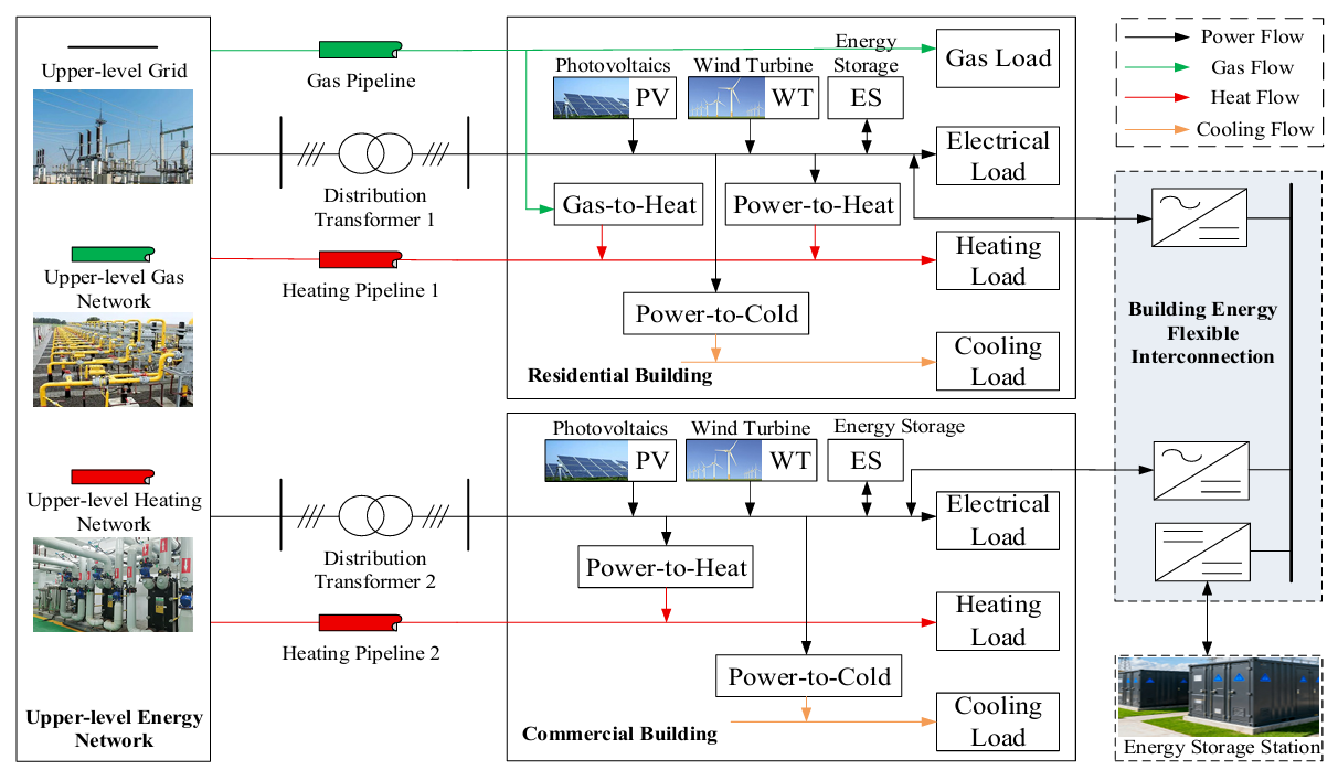
This study considers a flexible interconnection scenario for multi-type building energy systems involving multi-energy complementarity. The system structure is shown in Figure 1. It mainly includes cooling, thermal, electrical, and gas loads, photovoltaic (PV) units, and a wind turbine. (WT) units, energy storage systems (ESS), flexible interconnection devices (FID), as well as energy conversion devices such as gas-to-heat (G2H), power-to-heat (P2H), and power-to-cold (P2C).
2.2. Photovoltaic Model
A photovoltaic power generation system typically consists of three parts: the PV array module, the inverter, and the controller. The output power of the PV array is primarily determined by solar radiation energy and the operating temperature of the PV cells. The specific expression is as follows [18]:
|
```latex{P}_{PV}\left(t\right)={P}_{STC}\frac{{G}_{T}\left(t\right)}{{G}_{STC}}\left[1+{k}_{c}\left({T}_{c}\left(t\right)-{T}_{STC}\right)\right]``` |
(1) |
where: PPV(t) represents the PV output power; PSTC represents the maximum power under standard test conditions (incident irradiance GSTC = 1000 W/m2, reference ambient temperature TSTC = 25 °C); GT represents the actual solar irradiance at time t; GSTC represents the solar irradiance under standard test conditions; kc represents the power temperature coefficient; Tc represents the actual operating temperature of the PV modules; TSTC represents the operating temperature under standard test conditions.
2.3. Wind Turbine Model
The blades of a wind turbine capture part of the energy from the airflow and convert it into rotational kinetic energy, which is then further converted into electrical energy through the generator. Assuming no difference in wind speed acquisition between different units for now, the output power of the wind turbine needs to be characterized using a segmented curve, with the specific form as follows [19]:
|
```latexP_{WT}(\nu)=\begin{cases}0&&\nu<\nu_c\\\frac{\nu-\nu_c}{\nu_f-\nu_c}P_{WT}^N&&\nu_c\leq\nu<\nu_N\\P_{WT}^N&&\nu_N\leq\nu\leq\nu_f\\0&&\nu_f<\nu&\end{cases}``` |
(2) |
where: PWT(v) represents the wind power output; $$P_{WT}^N$$ represents the rated power of a single wind turbine unit; vc, vf, and vN represent the cut-in wind speed, cut-out wind speed, and rated wind speed, respectively.
If the microgrid contains N identical wind turbines, the average output power of wind power generation over a certain period T can be expressed as:
|
```latex{P}_{WT}={N}_{WT}{\int }_{0}^{T}{P}_{WT}\left(v\right)f\left(v\right)dv``` |
(3) |
|
```latexf\left(v\right)=1-{e}^{\left[-{\left(\frac{v}{c}\right)}^{k}\right]}``` |
(4) |
where: f(v) is the probability density function described using the two-parameter Weibull distribution, where k (k > 0) is the shape parameter of the distribution, and c (c > 1) is the scale parameter of the distribution.
2.4. Electrical Storage Model
To protect the storage battery and extend its service life as much as possible, it is necessary to avoid simultaneous charging and discharging of the battery. Therefore, constraints must be applied to its charging and discharging states as follows:
|
```latex0\le {B}_{ES}^{C}\left(t\right)+{B}_{ES}^{D}\left(t\right)\le 1``` |
(5) |
where: $${B}_{ES}^{C}\left(t\right)$$ and $${B}_{ES}^{D}\left(t\right)$$ are the charging state and discharging state of the energy storage device at time t, respectively, both taking values of 0 or 1; when $${B}_{ES}^{C}$$ = 0, it indicates the energy storage device is in the discharging state, and when $${B}_{ES}^{C}$$ = 1, it indicates the energy storage device is in the charging state. The meaning of $${B}_{ES}^{D}$$ is opposite to that of $${B}_{ES}^{C}$$.
In the energy storage device model, the influence of temperature on battery capacity is neglected, and the charging and discharging currents are assumed to remain constant over a unit time step. The state of charge (SOC) represents the ratio of the remaining capacity of the battery to its total capacity. When the battery is in the charging state, its SOC update formula is as follows [20]:
|
```latexS_{OC}(t+1)=S_{OC}(t)+\frac{\Delta t}{S_{ES}}\left[B_{ES}^C(t)P_{ES}^C(t)\eta_{ES}^C-\frac{B_{ES}^D(t)P_{ES}^D(t)}{\eta_{ES}^D}\right]``` |
(6) |
where: SOC(t + 1) and SOC(t) represent the remaining capacity of the battery at the corresponding time intervals, respectively; SES is the installed capacity of the energy storage system, in kWh; $$P_{ES}^C(t)$$ and $$P_{ES}^D(t)$$ are the charging power and discharging power at time interval t, respectively; $$\eta_{ES}^C$$ and $$\eta_{ES}^D$$ correspond to the charging efficiency and discharging efficiency of the battery, respectively.
2.4.1. Energy Storage Charge/Discharge Power Constraints
Considering that excessively high power may lead to safety hazards such as thermal runaway and internal short circuits in the energy storage device, the following constraints are imposed on the charge and discharge power of the energy storage device:
|
```latexP_{ES}^{\min} \leq P_{ES}(t) \leq P_{ES}^{\max}``` |
(7) |
where: $$P_{ES}^{\min}$$ and $$P_{ES}^{\max}$$ represent the lower and upper limits of the energy storage power constraint, respectively; PES(t) represents the charge/discharge power of the energy storage device at time t. When PES(t) is positive, it indicates the storage is discharging; when PES(t) is negative, it indicates the storage is charging.
2.4.2. Energy Storage State of Charge (SOC) Constraint
Considering that excessively high power may lead to safety hazards such as thermal runaway and internal short circuits in the energy storage device, the following constraints are imposed on the charge and discharge power of the energy storage device:
|
```latexS_{OC}^{\min}\leq S_{OC}(t)\leq S_{OC}^{\max}``` |
(8) |
where: SOC(t) is the state of charge of the energy storage device; $$S_{OC}^{\min}$$ and $$S_{OC}^{\max}$$ are the lower and upper limits of the state of charge, respectively.
Furthermore, after a complete time cycle, to ensure the cyclic operational stability of the energy storage, its state of charge needs to return to the initial value, specifically satisfying:
|
```latex{S}_{OC}\left[\left(n+1\right)T\right]={S}_{OC}\left(nT\right)``` |
(9) |
where: T represents a complete cycle. The above equation ensures that the energy storage capacity is equal at the beginning and end of the dispatch cycle, facilitating cyclic scheduling of the storage.
2.4.3. Energy Storage Ramp Power Constraint
To avoid excessive power fluctuations of the energy storage device affecting system stability, its ramp power needs to be constrained, with the specific form as follows:
|
```latex{P}_{ES}^{down}\Delta t\le \left|{P}_{ES}\left(t\right)-{P}_{ES}(t-1)\right|\le {P}_{ES}^{up}\Delta t``` |
(10) |
where: $${P}_{ES}^{up}$$ and $${P}_{ES}^{down}$$ are the upper and lower limits of the ramp rate, respectively.
2.5. Flexible Interconnection Device Model
Firstly, it is necessary to avoid the simultaneous occurrence of power inflow and outflow at the same port of the flexible interconnection device. Therefore, constraints must be applied to its states as follows:
|
```latex0\le {B}_{FID}^{in,i}\left(t\right)+{B}_{FID}^{out,i}\left(t\right)\le 1``` |
(11) |
where: $${B}_{FID}^{in,i}\left(t\right)$$ and $${B}_{FID}^{out,i}\left(t\right)$$ are the power inflow state and power outflow state of port i of the flexible interconnection device at time t, respectively, both taking values of 0 or 1; when $${B}_{FID}^{in,i}$$ = 0, it indicates that port i of the flexible interconnection device is in the power inflow state, and when $${B}_{FID}^{in,i}$$ = 1, it indicates that port i of the flexible interconnection device is in the power outflow state. The meaning of $${B}_{FID}^{out,i}$$ is opposite to that of $${B}_{FID}^{in,i}$$.
2.5.1. FID Power Balance Constraint
|
```latex\sum_{i=1}^N\eta_{FID}^{in}P_{FID}^{in,i}(t)=\sum_{j=1}^M\frac{P_{FID}^{out,j}(t)}{\eta_{FID}^{out}}``` |
(12) |
where: N is the number of ports with power inflow into the flexible interconnection device at time t; M is the number of ports with power outflow from the flexible interconnection device at time t; $$P_{FID}^{in,i}$$ is the inflow power at port i of the flexible interconnection device at time t; $$P_{FID}^{out,j}$$ is the outflow power at port j of the flexible interconnection device at time t; $$\eta_{FID}^{in}$$ and $$\eta_{FID}^{out}$$ correspond to the power inflow transmission efficiency and power outflow transmission efficiency of the flexible interconnection device, respectively.
2.5.2. Transmission Power Constraint
|
```latex0\le \left|{P}_{FID}^{t}\right|\le {P}_{FID}^{\max}``` |
(13) |
where: $${P}_{FID}^{\max}$$ is the maximum transmission power of the flexible interconnection device; PFID(t) is the transmission power of the flexible interconnection device during time interval t.
2.6. Energy Conversion Equipment Model
Without affecting the methodology of this paper, the ramp rates of the power-to-heat, power-to-cold, and gas-to-heat devices are temporarily not considered, and it is assumed that the energy conversion devices operate at. constant output within the minimum dispatch time interval. Start-stop control with “either 0 or 1” states is used for stepwise regulation. The energy consumption modeling of the energy conversion equipment is as follows.
The total power consumed through the power-to-heat device is:
|
```latexP_{E2H}(t)=\sum_{j=1}^{N_{E2H}}[B_{E2H}^j(t)P_{E2H}^j]``` |
(14) |
where: PE2H(t) represents the total power consumed by the power-to-heat device at time t; NE2H represents the total number of power-to-heat devices; $$P_{E2H}^j$$ represents the rated power of the j-th power-to-heat device; $$B_{E2H}^j(t)$$ represents the start-stop variable of the j-th power-to-heat device at time t, where $$B_{E2H}^j(t)$$ = 0 indicates the shutdown state, and $$B_{E2H}^j(t)$$ = 1 indicates the operating state.
Considering the electrical-to-thermal conversion efficiency, its output thermal power is as follows:
|
```latex{H}_{E2H}\left(t\right)={\eta }_{E2H}{P}_{E2H}\left(t\right)``` |
(15) |
where: HE2H(t) represents the output thermal power of the power-to-heat device at time t; ηE2H represents the electrical-to-thermal conversion efficiency of the power-to-heat device.
The total power consumed through the power-to-cold device is:
|
```latexP_{E2C}(t)=\sum_{j=1}^{N_{E2C}}\left[B_{E2C}^j(t)P_{E2C}^j\right]``` |
(16) |
where: PE2C(t) represents the total power consumed by the power-to-cold device at time t; NE2C represents the total number of power-to-cold devices; $$P_{E2C}^j$$ represents the rated power of the j-th power-to-cold device; $$B_{E2C}^j(t)$$ represents the start-stop variable of the j-th power-to-cold device at time t, where $$B_{E2C}^j(t)$$ = 0 indicates the shutdown state, and $$B_{E2C}^j(t)$$ = 1 indicates the operating state.
Considering the electrical-to-cooling conversion efficiency, its output cooling power is as follows:
|
```latex{C}_{E2C}\left(t\right)={C}_{OP}{P}_{E2C}\left(t\right)``` |
(17) |
where: CE2C(t) represents the output cooling power of the power-to-cold device at time t; COP represents the coefficient of performance of the power-to-cold device.
The output thermal power of the gas-to-heat device is:
|
```latex{H}_{G2H}\left(t\right)={\eta }_{G2H}{F}_{G2H}\left(t\right){Q}_{LHV}``` |
(18) |
where: HG2H(t) represents the output thermal power of the gas-to-heat device at time t; ηG2H represents the gas-to-thermal conversion efficiency of the gas-to-heat device; FG2H(t) represents the natural gas consumption of the gas-to-heat device at time t, in m3; QLHV represents the lower heating value of natural gas, taken as 37.62 MJ/Nm3 in this paper.
3. Bi-Level Optimization Model
3.1. Upper-Level Model
The upper-level model is responsible for solving the optimal configuration problem of minimizing the total lifecycle cost and full-chain carbon emissions of the. multi-building energy system over the planning period. Decision variables include the configured capacity of energy storage and the configured capacity of flexible interconnection devices.
3.1.1. Objective Function
The upper-level mathematical model can be expressed as:
|
```latex\text{min}{F}_{up}=\left\{{f}_{1}\left(x\right),{f}_{2}\left(x\right)\right\}``` |
(19) |
where: Fup is the objective function of the upper-level optimization configuration model; f1(x) is the system total lifecycle cost; f2(x) is the full-chain carbon emission.
The total lifecycle cost of the building energy system includes electricity sales revenue, energy purchase costs, investment costs, and operation and maintenance costs.
|
```latex{f}_{1}\left(x\right)={C}_{SE}-{C}_{BU}-{C}_{IN}-{C}_{OM}``` |
(20) |
where: CSE represents electricity sales revenue; CBE represents energy purchase cost; CIN represents investment cost; COM represents operation and maintenance cost.
|
```latexC_{SE}=Y\sum_{l=1}^kT_l\sum_{t=1}^{24}c_{SE}^EP_{SE}^E``` |
(21) |
where: Y is the planning horizon; k is the number of planning scenarios; Tl is the number of days in the l-th planning scenario of the year; $$c_{SE}^E(t)$$ represents the unit power electricity sales revenue at time t, in yuan/kW; $$P_{SE}^E(t)$$ represents the electricity sales power at time t, in kW.
|
```latexC_{BU}=Y\sum_{l=1}^kT_l\sum_{t=1}^{24}c_{buy}^E(t)P_{buy}^E(t)+c_{buy}^GV_{buy}^G(t)+c_{buy}^HH_{buy}^H(t)``` |
(22) |
where: $$c_{buy}^E(t)$$ represents the unit power electricity purchase cost at time t, in yuan/kW; $$P_{buy}^E(t)$$ represents the electricity purchase power at time t, in kW; $$c_{buy}^G(t)$$ represents the unit volume gas purchase cost at time t, in yuan/m3; $$V_{buy}^G(t)$$ represents the gas purchase volume at time t, in m3; $$c_{buy}^H(t)$$ represents the unit power heat purchase cost at time t, in yuan/kW; $$H_{buy}^H(t)$$ represents the heat purchase power at time t, in kW.
|
```latexC_{IN}=\sum_{l=1}^{k}T_{l}\sum_{t=1}^{24}(c_{ES}^{IN}S_{ES}^{IN}+c_{FID}^{IN}S_{FID}^{IN})``` |
(23) |
where: $$c_{ES}^{IN}$$ represents the unit capacity investment cost of energy storage, in yuan/kW; $$S_{ES}^{IN}$$ represents the configured capacity of energy storage, in kW; $$c_{FID}^{IN}$$ represents the unit power investment cost of the flexible interconnection device, in yuan/kW; $$P_{FID}^{IN}$$ represents the configured power of the flexible interconnection device, in kW.
|
```latexC_{OM}=Y\sum_{l=1}^kT_l\sum_{t=1}^{24}[c_{PV}^{OM}P_{PV}(t)+c_{WT}^{OM}P_{WT}(t)+B_{ES}^C(t)P_{ES}^C(t)\eta_{ES}^C+\frac{c_{ES}^{OM}B_{ES}^D(t)P_{ES}^D(t)}{\eta_{ES}^D}]``` |
(24) |
where: $$c_{PV}^{OM}$$ represents the unit power O&M cost of photovoltaics, in yuan/kW; $$c_{WT}^{OM}$$ represents the unit power O&M cost of wind turbines, in yuan/kW; $$c_{ES}^{OM}$$ represents the unit power O&M cost of energy storage, in yuan/kW.
The full-chain carbon emissions of the building energy system include carbon sources from grid electricity purchase, gas network gas purchase, and heat network. heat purchase. The total system carbon emissions equal the sum of the respective energy consumption multiplied through the corresponding dynamic carbon emission factors.
|
```latexf_2(x)=\sum_{l=1}^kT_l\sum_{t=1}^{24}e_E(t)P_{buy}^E(t)+e_G(t)V_{buy}^G(t)+e_H(t)P_{buy}^H(t)``` |
(25) |
where: eE(t) represents the carbon emission factor for grid electricity purchase at time t, in kgCO2/kW; eG(t) represents the carbon emission factor for gas network gas purchase at time t, in kgCO2/kW; eH(t) represents the carbon emission factor for heat network heat purchase at time t, in kgCO2/kW.
3.1.2. Constraints
Equipment Installation Capacity Constraints
|
```latex0\le {S}_{ES}\le {S}_{ES}^{\max}``` |
(26) |
|
```latex0\le {S}_{FID}\le {S}_{FID}^{\max}``` |
(27) |
where: $${S}_{ES}^{\max}$$ is the upper limit of the energy storage system installation capacity, in kWh; SFID is the installation capacity of the flexible interconnection device, in kWh; $${S}_{FID}^{\max}$$ is the upper limit of the flexible interconnection device installation capacity, in kWh.
System Electrical Power Balance Constraint
|
```latex\begin{aligned}&P_{PV}(t)+P_{WT}(t)+P_{buy}^{E}(t)+B_{ES}^{D}(t)\eta_{ES}^{D}P_{ES}^{D}(t)+\sum_{j=1}^{M}\frac{P_{FID}^{out,j}(t)}{\eta_{FID}^{out}}\\&=P_L(t)+\eta_{E2H}P_{E2H}(t)+C_{OP}P_{E2C}(t)+B_{ES}^C(t)P_{ES}^C(t)/\eta_{ES}^C+\sum_{i=1}^N\eta_{FID}^{in}P_{FID}^{in,i}(t)\end{aligned}``` |
(28) |
System Thermal Power Balance Constraint
|
```latex{H}_{buy}^{H}\left(t\right)+{H}_{G2H}\left(t\right)+{H}_{E2H}\left(t\right)={H}_{L}\left(t\right)``` |
(29) |
where: $${H}_{buy}^{H}\left(t\right)$$ represents the purchased heat power from the heat network at time t; HL(t) represents the system thermal load power at time t.
System Cooling Power Balance Constraint
|
```latex{C}_{E2C}\left(t\right)={C}_{L}\left(t\right)``` |
(30) |
where: CL(t) represents the system cooling load power at time t.
Photovoltaic and Wind Power Output Constraints
|
```latex0\le {P}_{WT}\left(t\right)\le {P}_{WT}^{pre}\left(t\right)``` |
(31) |
|
```latex0\le {P}_{PV}\left(t\right)\le {P}_{PV}^{pre}\left(t\right)``` |
(32) |
where: $${P}_{PV}^{pre}\left(t\right)$$ represents the forecast PV output power at time t; $${P}_{WT}^{pre}\left(t\right)$$ represents the forecast wind power output at time t.
3.2. Lower-Level Model
The lower-level model takes the optimal configuration solution from the upper-level model as constraints and is responsible for solving the optimal operation problem of maximizing the renewable energy self-consumption rate and minimizing the typical daily comprehensive operation cost of the multi-building energy system. Decision variables include the power purchased. from the upper-level grid, heat input power from the upper-level heat network, gas volume input from the upper-level gas network, power consumed by power-to-heat devices, power consumed by power-to-cold devices, heat output power from gas-to-heat devices, charge/discharge power of energy storage, and power transferred by flexible interconnection devices.
3.2.1. Objective Function
The lower-level mathematical model can be expressed as:
|
```latex\min F_{down}=\begin{Bmatrix}-f_3(x),f_4(x)\end{Bmatrix}``` |
(33) |
where: Fdown is the objective function of the lower-level optimization configuration model; f3(x) is the renewable energy self-consumption rate; f4(x) is the typical daily comprehensive operation cost.
The renewable energy self-consumption rate of the building energy system is the ratio of the sum of the electricity directly supplied to the building. loads by renewable energy generation and the electricity indirectly supplied to building loads via energy storage, after being stored, to the total building load:
|
```latexR_{new}=\sum_{l=1}^kT_l\sum_{t=1}^{24}\frac{P_L^{PV}(t)+P_L^{WT}(t)+P_L^{ES,new}(t)}{P_L^{all}(t)}``` |
(34) |
where: Rnew is the renewable energy self-consumption rate; $$P_L^{PV}(t)$$ represents the PV generation directly supplying the building load at time t; $$P_L^{WT}(t)$$ represents the wind power generation directly supplying the building load at time t; $$P_L^{ES,new}(t)$$ represents the renewable energy generation supplied to the building load via energy storage after being stored at time t; $$P_L^{all}(t)$$ represents the total building load at time t.
The typical daily comprehensive operation cost of the building energy system includes electricity sales revenue, energy purchase cost, and wind/solar curtailment penalty cost.
|
```latex\left\{\begin{array}{l}{C}_{SE}^{day} = \sum\limits_{t=1}^{24} {c}_{SE}^{E}{P}_{SE}^{E} \\{C}_{BU}^{day} = \sum\limits_{t=1}^{24} {c}_{buy}^{E}\left(t\right){P}_{buy}^{E}\left(t\right) + {c}_{buy}^{G}{V}_{buy}^{G}\left(t\right) + {c}_{buy}^{H}{H}_{buy}^{H}\left(t\right) \\{C}_{PN}^{day} = \sum\limits_{t=1}^{24} \left( {c}_{PV}^{PN}{P}_{PV}^{PN} + {c}_{WT}^{PN}{P}_{WT}^{PN} \right)\end{array}\right.``` |
(35) |
where: $$C_{SE}^{day}$$ represents the daily electricity sales revenue; $${C}_{BU}^{day}$$ represents the daily energy purchase cost; $${C}_{PN}^{day}$$ represents the daily wind and solar curtailment penalty cost; $${c}_{PV}^{PN}$$ represents the unit power curtailment penalty cost for PV, in yuan/kW; $${c}_{WT}^{PN}$$ represents the unit power curtailment penalty cost for WT, in yuan/kW; $${P}_{PV}^{PN}$$ represents the curtailed PV power, in kW; $${P}_{WT}^{PN}$$ represents the curtailed wind power, in kW.
3.2.2. Constraints
Shiftable Load Constraint
Only designated shiftable loads can participate in demand response. The shiftable load within the response period cannot exceed the specified limit for shiftable loads. The daily total of shiftable loads is only allowed to be shifted in time sequence, not increased or decreased.
|
```latex0\le {m}_{L}^{T}\left(t\right)\le {M}_{L}^{T}\left(t\right)``` |
(36) |
|
```latex{m}_{L}^{T}\left(t\right){P}_{L}\left(t\right)+{m}_{L}^{N}\left(t\right){P}_{L}\left(t\right)={P}_{L}\left(t\right)``` |
(37) |
where: $${m}_{L}^{T}\left(t\right)$$ represents the proportion of shiftable load at time t; $${M}_{L}^{T}\left(t\right)$$ represents the upper limit of the shiftable load proportion at time t; $${m}_{L}^{N}\left(t\right)$$ represents the proportion of non-interruptible load at time t.
Interaction Power Constraint
Excessively high reverse power flow from renewable energy generation can adversely affect grid stability; therefore, there are restrictions on the reverse power flow from renewable sources.
|
```latex-{P}_{grid}^{sell}\le {P}_{buy}^{E}\left(t\right)\le {P}_{grid}^{buy}``` |
(38) |
where: $${P}_{grid}^{sell}$$ represents the maximum reverse power sold from the building energy system to the external grid; $${P}_{grid}^{buy}$$ represents the maximum power purchased by the building energy system.
4. Model Solution
4.1. Solution Algorithm
Unlike general single-objective optimization problems, multi-objective optimization problems cannot find a single optimal solution. According to Pareto theory, the optimal solution is a set of solutions. and the curve formed in the solution space is called the Pareto front. First, the multi-objective optimization problem of the building energy system is described as follows:
|
```latex\begin{cases}\min[F_{up},F_{down}]\\h_i(x)=0,\quad i=1,2,3,...,p\\g_j^{\min}(x)\leq g_j(x)\leq g_j^{\max}(x),\quad j=1,2,3,...,q&\end{cases}``` |
(39) |
where: hi(x) = 0 are equality constraints, and $$g_j^{\min}(x)\leq g_1(x)\leq g_j^{\max}(x)$$ are inequality constraints. Traditional multi-objective optimization algorithms combine multiple objectives into a single objective function according to certain weight coefficients. However, the weight coefficients are often determined by empirical values. Given the deep coupling of core contradictions in building energy systems, using weight coefficients to solve building energy system optimization problems yields unsatisfactory results.
Therefore, this paper adopts a hybrid solution strategy combining Lévy flight distribution and a good point set with NSGA-II to solve the multi-objective bi-level optimization configuration problem of the building energy system. The model solution process is shown in Figure 2. The good point set is used for population initialization, which can generate an initial population uniformly distributed within the search space, clearly improving initial population diversity and thus avoiding premature convergence to local optima. The model parameters are set as follows: initial population size is 200, maximum number of iterations is 1000. The crossover probability is 0.8, and the mutation probability is 0.2. The parameters α and β for the Lévy distribution are dynamic optimization parameters. In the early iterations, α is set to 1.5 and β to 0.5; in the later iterations, α is set to 0.5 and β to 1.5.
Among them, the Lévy distribution is used to improve the mutation operator. It possesses the characteristics of short-distance, small-step exploration and long-distance, large-step jumps, which can effectively balance the local refined search capability and global exploration capability of NSGA-II. To prevent the large steps of the Lévy distribution from disrupting convergence in the later stages of the algorithm, parameters can be dynamically adjusted: in the early iterations, β takes a smaller value and. α is larger, favoring more large steps to enhance global exploration; in the later iterations, β increases and α decreases, favoring small steps for fine-tuning and focusing on local development. For the complex non-convex search space formed by multi-energy flow coupling, flexible device output constraints, and regional load fluctuations in the multi-building interconnected system, this improvement helps the algorithm effectively escape local optima and increases the probability of finding the global Pareto optimal solution.
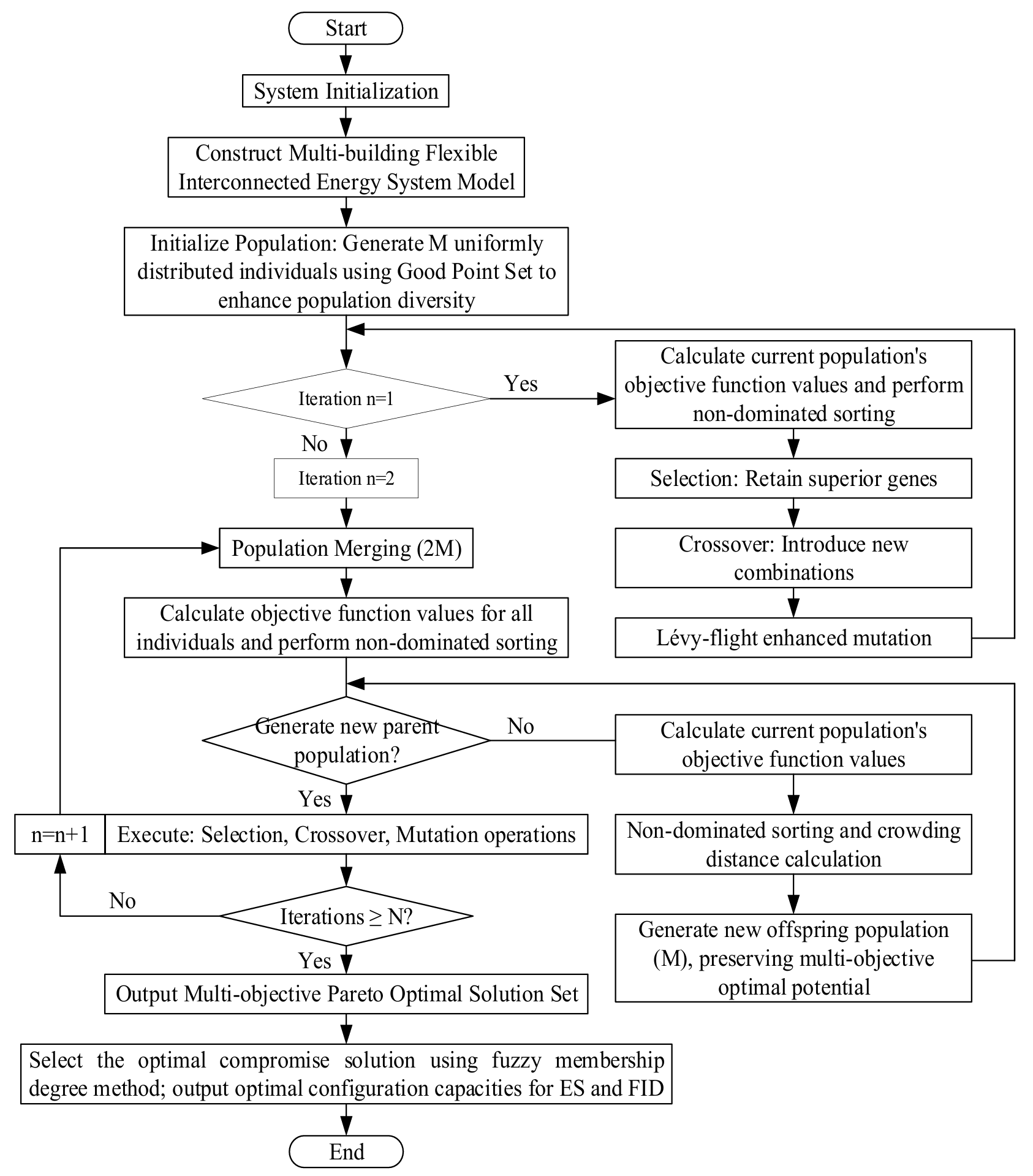
Figure 2. Figure caption should comprise a brief title (not on the figure itself) and a description of the illustration.
4.2. Final Solution Selection
The Pareto front obtained through the optimization algorithm is a set of non-dominated solutions that do not dominate each other; there is no single solution that is optimal for all objectives. The decision-maker needs to select a configuration based on actual planning and emphasis. To obtain the final operation scheme. It is necessary to select a suitable solution from the Pareto solution set. After obtaining the Pareto optimal front, the fuzzy membership function is used to evaluate the decision-maker’s comprehensive satisfaction with each non-dominated solution, and the solution with the highest comprehensive membership degree is selected as the optimal compromise solution.
The fuzzy membership function is defined as:
|
```latex\Phi=\sum_{i=1}^I\varphi_i``` |
(40) |
| ```latex\varphi_i=\begin{cases}1&m_i\leq m_i^{\min}\\\frac{m_i^{\max}-m_i}{m_i^{\max}-m_i^{\min}}&m_i^{\min}<m_i<m_i^{\max}\\0&m_i\geq m_i^{\max}&&\end{cases}``` |
(41) |
where: mi is the value of the i-th objective function; $$m_i^{\min}$$ and $$m_i^{\max}$$ are the minimum and maximum values of the i-th objective function, respectively; Φ is the comprehensive membership degree of the objective functions.
5. Case Study Analysis
5.1. Basic Data
This paper uses the hybrid solution strategy combining Lévy flight distribution and a good point set with NSGA-II to solve the multi-objective bi-level optimization configuration problem of the building energy system.
Table 1 shows the system parameters, including basic building parameters, carbon emission parameters, energy conversion parameters, constraint parameters, and cost parameters. Table 2 shows the time-of-use electricity prices for commercial electricity in Beijing during summer and winter.
Table 1. System Parameters.
|
Category |
Parameter Name |
Symbol |
Residential Building |
Commercial Building |
Unit |
|---|---|---|---|---|---|
|
Basic Building |
Floor Area |
- |
30,000 |
10,000 |
m2 |
|
PV Installed Capacity |
PPV |
200 |
400 |
kW |
|
|
WT Installed Capacity |
PWT |
100 |
200 |
kW |
|
|
Carbon Emission |
Grid Electricity Purchase Emission Factor |
eE |
0.80 |
0.80 |
kgCO2/kWh |
|
Gas Network Purchase Emission Factor |
eG |
0.58 |
- |
kgCO2/kWh |
|
|
Heat Network Purchase Emission Factor |
eH |
0.25 |
0.25 |
kgCO2/kWh |
|
|
Energy Conversion |
Flexible Interconnection Trans. Efficiency |
ηFID |
0.95 |
0.95 |
- |
|
Energy Storage Charging Efficiency |
$$\eta_{ES}^{C}$$ |
0.92 |
0.92 |
- |
|
|
Energy Storage Discharging Efficiency |
$$\eta_{ES}^{D}$$ |
0.88 |
0.88 |
- |
|
|
Power-to-Heat Conversion Efficiency |
ηE2H |
0.95 |
0.95 |
- |
|
|
Coefficient of Performance (Cooling) |
COP |
3.0 |
4.0 |
- |
|
|
Gas-to-Heat Conversion Efficiency |
ηG2H |
0.9 |
- |
- |
|
|
Constraint |
Energy Storage SOC Lower Limit |
$$S_{OC}^{\min}$$ |
0.15 |
0.15 |
- |
|
Energy Storage SOC Upper Limit |
$$S_{OC}^{\max}$$ |
0.95 |
0.95 |
- |
|
|
Max. Charge/Discharge Power of ES |
$$P_{ES}^{\max}$$ |
250 |
250 |
kW |
|
|
Min. Charge/Discharge Power of ES |
$$P_{ES}^{\min}$$ |
10 |
10 |
kW |
|
|
FID Max. Transmission Power |
$$P_{FID}^{\max}$$ |
200 |
200 |
kW |
|
|
FID Min. Transmission Power |
$$P_{FID}^{\min}$$ |
10 |
10 |
kW |
|
|
Shiftable Load Proportion Upper Limit |
$$M_L^T$$ |
0.15 |
0.10 |
- |
|
|
Cost Parameters |
ES Unit Capacity Investment Cost |
$$c_{ES}^{IN}$$ |
1500 |
1500 |
yuan/kWh |
|
FID Unit Power Investment Cost |
$$c_{FID}^{IN}$$ |
1000 |
1000 |
yuan/kW |
|
|
PV Unit Power O&M Cost |
$$c_{PV}^{OM}$$ |
20 |
20 |
yuan/kW |
|
|
WT Unit Power O&M Cost |
$$c_{WT}^{OM}$$ |
20 |
20 |
yuan/kW |
|
|
ES Unit Power O&M Cost |
$$c_{ES}^{OM}$$ |
80 |
80 |
yuan/kW |
|
|
FID Unit Power O&M Cost |
$$c_{FID}^{OM}$$ |
50 |
50 |
yuan/kW |
|
|
Unit Power Wind/Solar Curtailment Penalty Cost |
cPN |
0.45 |
0.45 |
yuan/kWh |
Note on currency: All costs in this paper are denominated in Chinese Yuan (CNY). For international reference, the average exchange rates in 2025 were 1 CNY = 0.1400 USD (1 USD = 7.1429 CNY) and 1 CNY = 0.1235 EUR (1 EUR = 8.0965 CNY), based on the People’s Bank of China official data.
Table 2. Commercial Electricity Time-of-Use Prices (yuan/kWh).
|
Season |
Period Type |
Time Periods |
Purchase Price |
Sale Price |
|---|---|---|---|---|
|
Summer |
Peak |
11:00–13:00, 16:00–17:00 |
1.6816 |
0.3913 |
|
High |
10:00–11:00, 17:00–22:00 |
1.4013 |
0.3913 |
|
|
Normal |
7:00–10:00, 13:00–16:00, 22:00–23:00 |
0.7785 |
0.3913 |
|
|
Low |
23:00–7:00 next day |
0.2336 |
0.3913 |
|
|
Winter |
Peak |
18:00–21:00 |
1.6816 |
0.3913 |
|
High |
10:00–13:00, 17:00–18:00, 21:00–22:00 |
1.4013 |
0.3913 |
|
|
Normal |
7:00–10:00, 13:00–17:00, 22:00–23:00 |
0.7785 |
0.3913 |
|
|
Low |
23:00–7:00 next day |
0.2336 |
0.3913 |
5.2. Simulation and Analysis
The selection of research data directly affects the optimization configuration and multi-objective evaluation results. Typically, the more representative the research data, the more reasonable the optimization configuration results and the closer they are to actual operation. Therefore, based on Beijing’s climate characteristics and building. load patterns, this paper selects two types of typical days—summer sunny day and winter sunny day—as simulation scenarios for case study analysis, which can fully verify the system’s adaptability under different operating conditions. The simulation analysis takes the unit time interval Δt as 1 h. The configuration results and performance metrics for different scenarios are presented in Table 3.
Table 3. Configuration Results and Indicators under Different Scenarios.
|
Configuration Method |
Energy Storage |
Flexible Interconnection Device |
Operation Mode |
|---|---|---|---|
|
Single-Building Independent |
Residential: 600 kW |
\ |
Single-Building Autonomous Dispatch |
|
Commercial: 600 kW |
|||
|
Multi-Building Interconnected |
Public: 500 kW |
Public: 200 kW |
Cross-Building Energy Synergy |
5.2.1. Summer Typical Day Operation Results
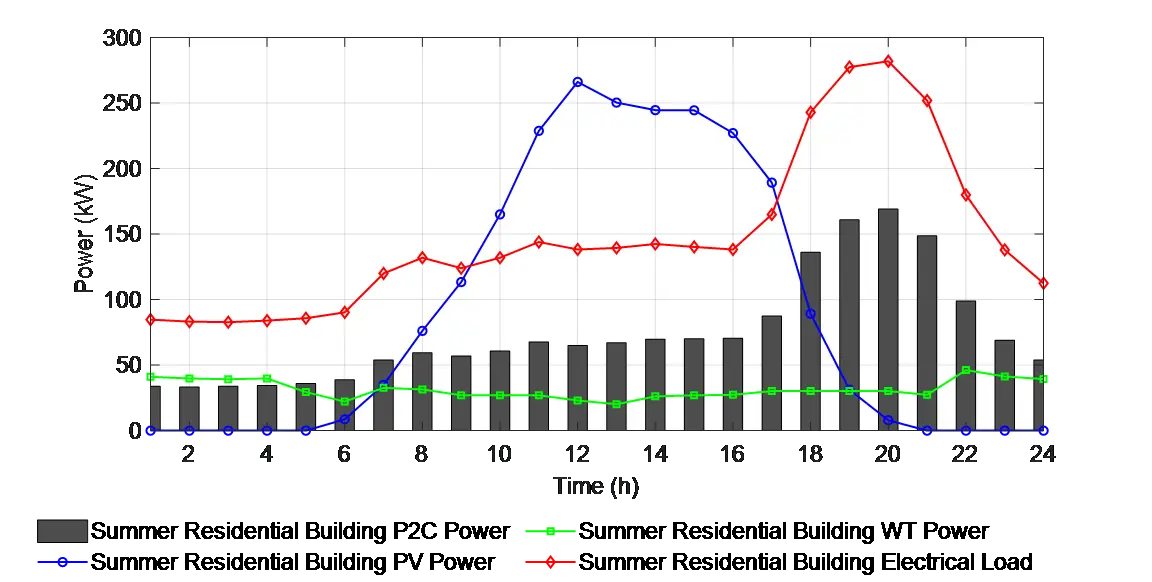
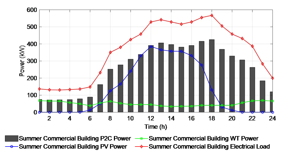
The source-load curves for civil and commercial buildings in summer are shown in Figure 3. On a typical summer sunny day, the residential building’s nighttime electricity peak and the commercial building’s daytime cooling load peak are temporally and spatially separated. The commercial building’s PV output during the day exceeds its own load demand, while the residential building lacks sufficient renewable energy output at night, leading to the coexistence of energy surplus and shortage in the building cluster.
 |
| (a) |
 |
| (b) |
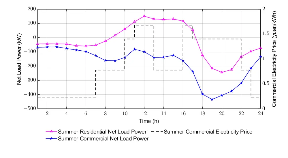 |
| (c) |
Figure 3. (a) Summer Residential Apartment Building Wind/PV Generation and Load Curve; (b) Summer Commercial Building Wind/PV Generation and Load Curve; (c) Summer Residential Apartment and Commercial Building Net Load Curve and Commercial Electricity Price.
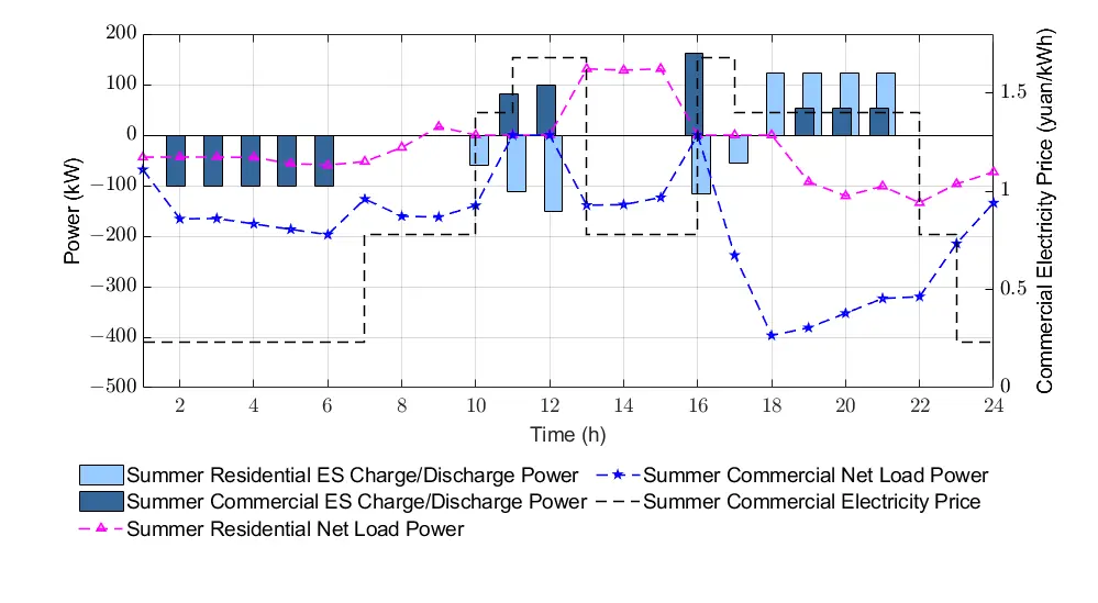
Single buildings cannot achieve load complementarity, resulting in the need to purchase expensive electricity during their respective peak periods. If single-building autonomous dispatch aims to achieve economical, low-carbon, and high proportion of renewable energy consumption, it must rely on purchasing electricity or large-capacity energy storage charging/discharging, inevitably leading to poor economy, low renewable energy consumption rate, and high carbon emissions. The optimized summer building source-load curves and energy storage operation status are illustrated in Figure 4.
 |
| (a) |
 |
| (b) |
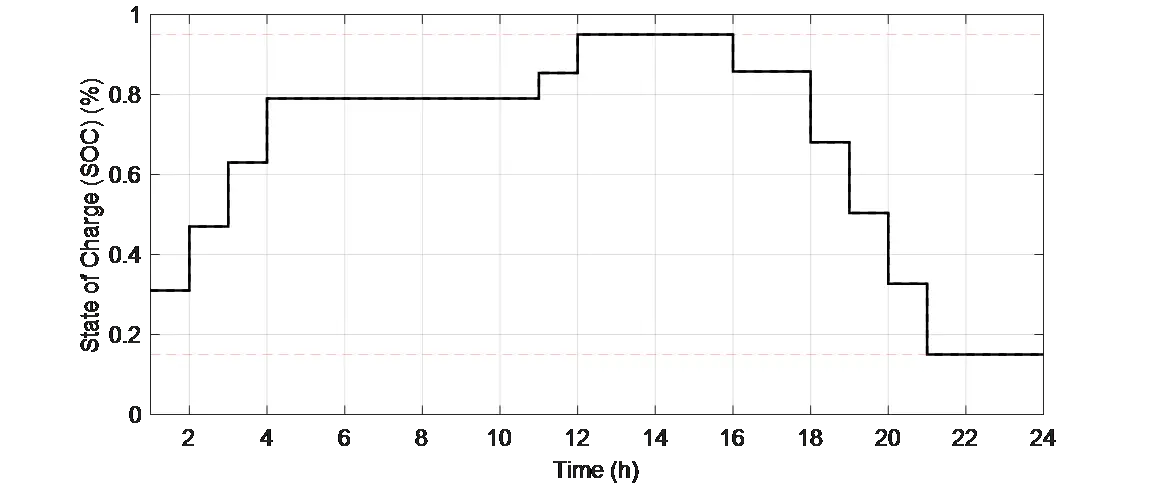 |
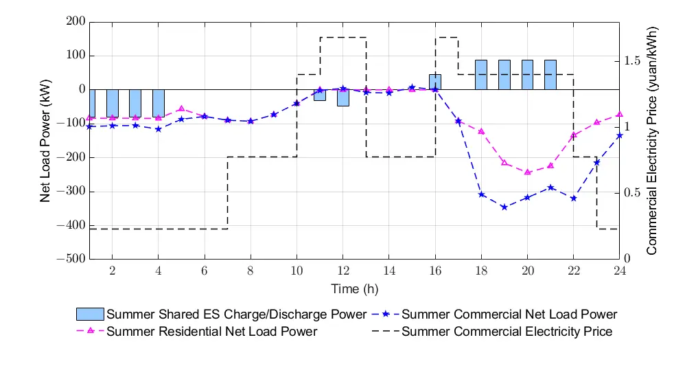
| (c) |
Figure 4. (a) Optimized Summer Residential Apartment and Commercial Building Net Load Curve and Commercial Electricity Price (Single-Building Independent Configuration); (b) Optimized Summer Residential Apartment and Commercial Building Net Load Curve and Commercial Electricity Price (Multi-Building Interconnected Configuration); (c) Energy Storage SOC Variation Curve under Multi-Building Interconnection.
5.2.2. Winter Typical Day Operation Results
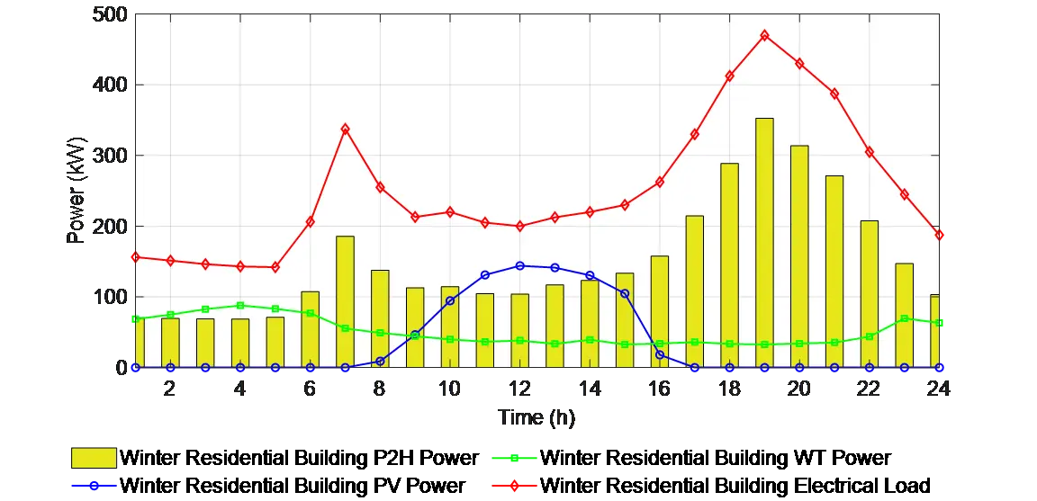
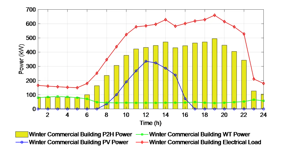
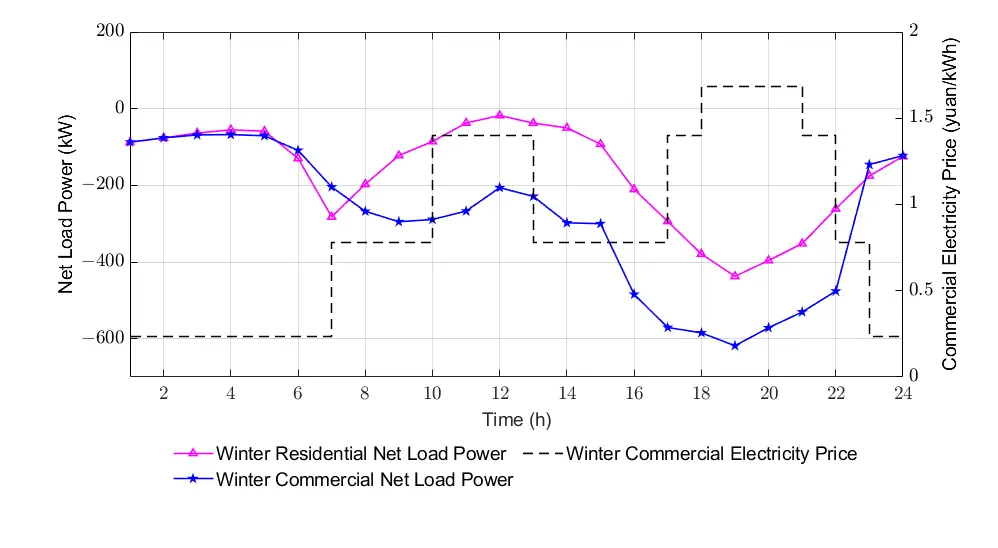
The source-load curves for civil and commercial buildings in winter are shown in Figure 5. On a typical winter sunny day, PV output is insufficient, and the heating load pressure is high. Winter PV output duration is shorter, and intensity is lower, resulting in insufficient average daily renewable energy output. Furthermore, residential morning and evening heating load peaks rely on power-to-heat or gas-to-heat, which overlap with peak electricity prices, jointly driving up operating costs.
 |
| (a) |
 |
| (b) |
 |
| (c) |
Figure 5. (a) Winter Residential Apartment Building Wind/PV Generation and Load Curve; (b) Winter Commercial Building Wind/PV Generation and Load Curve; (c) Winter Residential Apartment and Commercial Building Net Load Curve and Commercial Electricity Price.
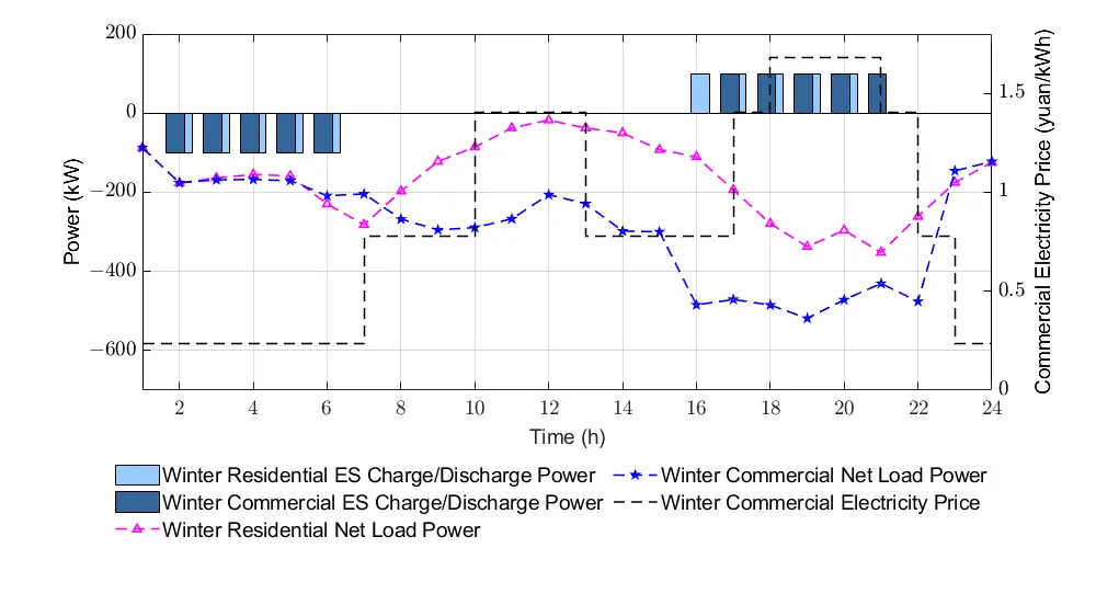
This leads to poor system economy and high carbon emissions. The optimized winter building source-load curves and energy storage operation status are illustrated in Figure 6.
 |
| (a) |
 |
| (b) |
 |
| (c) |
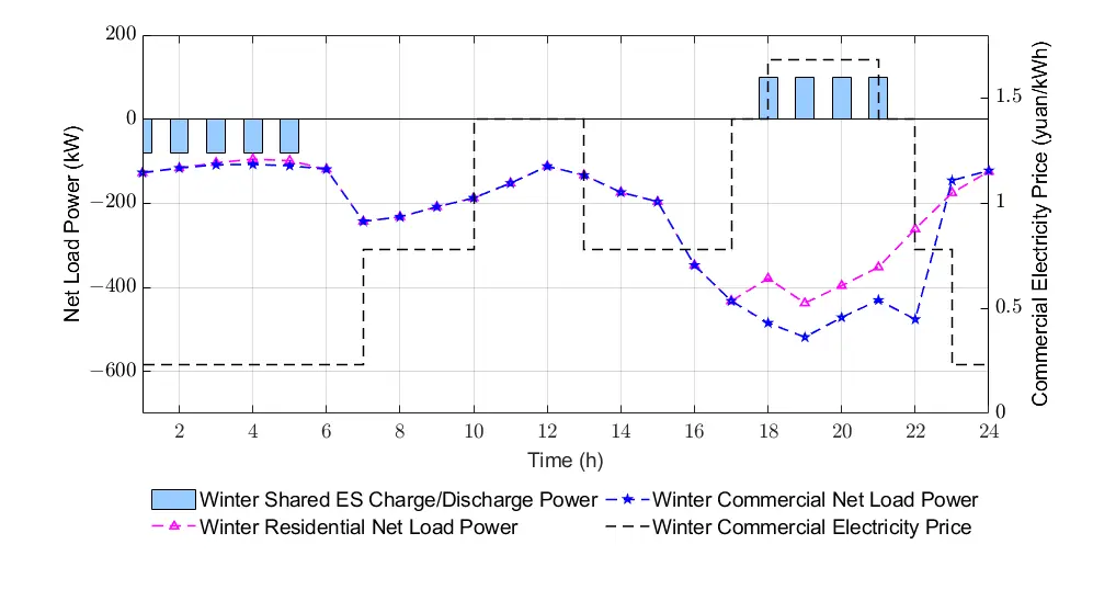
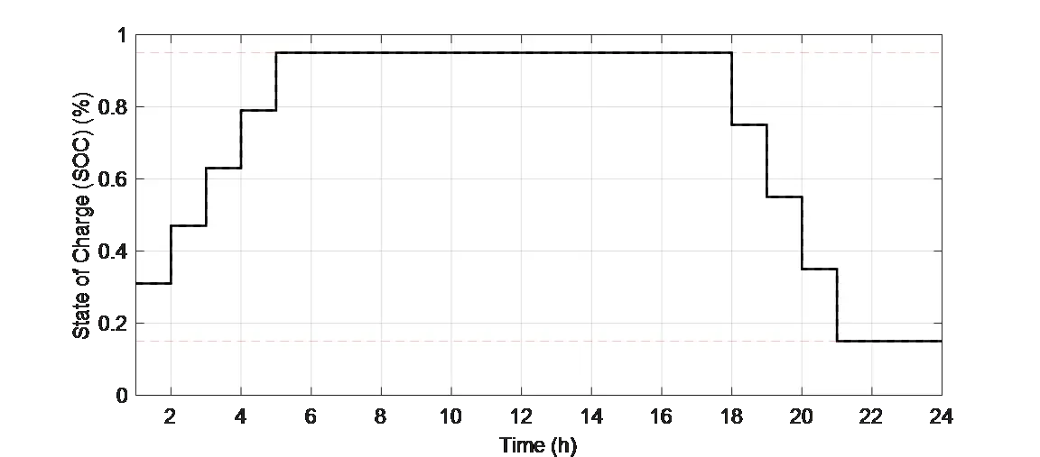
Figure 6. (a) Optimized Winter Residential Apartment and Commercial Building Net Load Curve and Commercial Electricity Price (Single-Building Independent Configuration); (b) Optimized Winter Residential Apartment and Commercial Building Net Load Curve and Commercial Electricity Price (Multi-Building Interconnected Configuration); (c) Energy Storage SOC Variation Curve under Multi-Building Interconnection.
From the simulation results, it can be seen that in terms of renewable energy self-consumption rate, under the single-building independent configuration scenario on a typical summer day, the self-consumption rate is 82.06%, which increases to 96.20% under the multi-building interconnected configuration scenario. This optimization stems from the period of 10:00–16:00 when the commercial building has surplus PV output. The flexible interconnection device transmits the residential building’s PV power to the commercial building, while the shared energy storage stores the PV energy not immediately consumed through the residential building during this period and releases it during the residential electricity consumption peak from 19:00–23:00. This addresses the issues of residential building PV curtailment during the day and commercial building electricity shortage at night under the single-building independent configuration, achieving efficient cross-building utilization of clean energy. On the typical winter day, due to insufficient average daily renewable energy output and high electricity consumption, renewable energy is almost entirely self-consumed. In terms of typical daily operation cost, the cost under the single-building independent configuration scenario on a typical summer day is 4888 yuan, which decreases to 4456 yuan under the multi-building interconnected configuration scenario, representing a relative reduction of 8.83%. The cost reduction originates from the grid peak price periods of 11:00–13:00 and 16:00–17:00, where the multi-building interconnected configuration reduces peak electricity purchases and lowers wind/PV curtailment. penalty costs through shared energy storage discharge and energy transfer via flexible interconnection devices. The single-building independent configuration has a larger energy storage capacity, thus achieving some improvement through peak-valley arbitrage revenue, but its total lifecycle cost is higher. On a typical winter day, the operation cost under the single-building independent configuration scenario is 10,782 yuan, compared to 11,505 yuan under the multi-building interconnected configuration scenario. The cost difference is primarily reflected in the larger energy storage capacity of the single-building independent configuration scenario, which yields more revenue through peak-valley arbitrage. In terms of carbon emissions, on the typical summer day, the daily carbon emission under the single-building independent configuration scenario is 4.42 tCO2, which decreases to 3.97 tCO2 under the multi-building interconnected configuration scenario, representing a relative reduction of 10.18% in carbon emissions. On a typical winter day, the daily carbon emission under the single-building independent configuration scenario is 8.92 tCO2, compared to 8.77 tCO2 under the multi-building interconnected configuration scenario, mainly due to minor differences caused by equipment efficiency. Furthermore, the peak-valley difference of the building energy system’s net load is reduced, primarily because the flexible interconnection device and energy storage enable dynamic capacity increase and power transmission during mismatched periods, which both smooths the commercial building load fluctuations and alleviate the power supply pressure on the upstream transformer of the commercial building.
6. Conclusions
This paper establishes a bi-level optimization model for a multi-building flexible interconnected energy system that considers cooling-thermal-electrical-gas multi-energy complementarity. The upper level focuses on optimizing equipment configuration to minimize total lifecycle costs and full-chain carbon emissions. The lower level concentrates on operational strategy optimization, targeting the maximization of the renewable energy self-consumption rate and the minimization of the typical daily operational cost. By employing a hybrid solution strategy that integrates Lévy flight distribution and good point sets with NSGA-II, efficient model solving and Pareto front acquisition are realized. Simulation results. indicate that, compared to the single-building independent configuration scheme, the multi-building flexible interconnection scheme demonstrates pronounced advantages in the typical summer day scenario: the renewable energy self-consumption rate increases from 82.06% to 96.20%, the typical daily operational cost is reduced by 8.83%, and carbon emissions are lowered by 10.18%. On a typical winter day, constrained by insufficient renewable energy output, the improvements in operational costs and carbon emissions are more modest. Nevertheless, the system can still achieve peak shaving and optimized allocation of energy resources through flexible interconnection and shared energy storage.
This study proposes a bi-level optimization framework coordinating planning and operation, which demonstrates more systematic optimization capabilities in planning-operation collaborative decision-making compared to existing research that focuses on single-stage or single-building scenarios. Future research may further explore directions such as robust optimization under multiple uncertainties, cross-regional collaborative dispatch, and the integration of intelligent algorithms. This method provides a theoretical foundation and engineering reference for the low-carbon and economic planning of regional building energy systems, supporting their transition toward greater flexibility, efficiency, and sustainability.
Statement of the Use of Generative AI and AI-Assisted Technologies in the Writing Process
During the preparation of this manuscript, the author(s) used DeepSeek in order to check the English grammar. After using this tool, the author(s) reviewed and edited the content as needed and take(s) full responsibility for the content of the published article.
Acknowledgments
The authors acknowledge the financial support from the National Key R&D Program of China, and thank the National Center of Technology Innovation for Green and Low-Carbon Building for providing the experimental platform.
Author Contributions
Conceptualization, W.W. and J.H.; Methodology, W.W. and X.X.; Software S.L., Validation, W.W. and S.L.; Formal Analysis S.L., Investigation B.L., Resources W.W., Data Curation B.L., Writing—Original Draft Preparation W.W., Writing—Review & Editing W.W., Visualization W.W., Supervision J.H., Project Administration X.X., Funding Acquisition, X.X.
Ethics Statement
Not applicable.
Informed Consent Statement
Not applicable.
Data Availability Statement
Some or all data, models, or code that support the findings of this study are available from the corresponding author upon reasonable request.
Funding
This research was supported by the National Key R&D Program of China (Grant No. 2024YFC3810105).
Declaration of Competing Interest
The authors declare that they have no known competing financial interests or personal relationships that could have appeared to influence the work reported in this paper.
References
- Liu X, Liu X, Jiang Y, Zhang T, Hao B. Photovoltaics and Energy Storage Integrated Flexible Direct Current Distribution Systems of Buildings: Definition, Technology Review, and Application. CSEE J. Power Energy Syst. 2022, 9, 829–845. DOI:10.17775/CSEEJPES.2022.04850 [Google Scholar]
- Huang W, Zhang X, Li K, Zhang N, Strbac G, Kang C. Resilience Oriented Planning of Urban Multi-Energy Systems with Generalized Energy Storage Sources. IEEE Trans. Power Syst. 2022, 37, 2906–2918. DOI:10.1109/TPWRS.2021.3123074 [Google Scholar]
- Wang W, Huo Q, Liu Q, Ni J, Zhu J, Wei T. Energy Optimal Dispatching of Ports Multi-Energy Integrated System Considering Optimal Carbon Flow. IEEE Trans. Intell. Transp. Syst. 2024, 25, 4181–4191. DOI:10.1109/TITS.2023.3336998 [Google Scholar]
- Hossain J, Shareef H, Hossain MA, Kalam A, Kadir AFA. Hybrid PV and Battery System Sizing for Commercial Buildings in Malaysia: A Case Study of FKE-2 Building in UTeM. IEEE Trans. Ind. Appl. 2024, 60, 4933–4945. DOI:10.1109/TIA.2024.3353714 [Google Scholar]
- Zhao H, Xu Z, Wu J, Liu F, Guan X. A Hierarchical Framework-Based Coordinated Optimization of Building HVAC Systems and EVs. IEEE Trans. Autom. Sci. Eng. 2025, 22, 6530–6542. DOI:10.1109/TASE.2024.344690 [Google Scholar]
- Yang Y, Shi J, Wang D, Wu C, Han Z. Net-Zero Scheduling of Multi-Energy Building Energy Systems: A Learning-Based Robust Optimization Approach with Statistical Guarantees. IEEE Trans. Sustain. Energy 2024, 15, 2675–2689. DOI:10.1109/TSTE.2024.3437210 [Google Scholar]
- Han J, Fang Y, Li Y, Du E, Zhang N. Optimal Planning of Multi-Microgrid System with Shared Energy Storage Based on Capacity Leasing and Energy Sharing. IEEE Trans. Smart Grid 2025, 16, 16–31. DOI:10.1109/TSG.2024.3452064 [Google Scholar]
- Zhang H, Li Z, Xue Y, Chang X, Su J, Wang P, et al. A Stochastic Bi-Level Optimal Allocation Approach of Intelligent Buildings Considering Energy Storage Sharing Services. IEEE Trans. Consum. Electron. 2024, 70, 5142–5153. DOI:10.1109/TCE.2024.3412803 [Google Scholar]
- Sharma S, Verma A, Xu Y, Panigrahi BK. Robustly Coordinated Bi-Level Energy Management of a Multi-Energy Building Under Multiple Uncertainties. IEEE Trans. Sustain. Energy 2021, 12, 3–13. DOI:10.1109/TSTE.2019.2962826 [Google Scholar]
- Sun Q, Wu Z, Gu W, Zhang X, Liu P. Tri-Level Multi-Energy System Planning Method for Zero Energy Buildings Considering Long- and Short-Term Uncertainties. IEEE Trans. on Sustainable Energy 2023, 14, 339–355. DOI: 10.1109/TSTE.2022.3212168 [Google Scholar]
- Nikkhah S, Allahham A, Royapoor M, Bialek JW, Giaouris D. Optimising Building-to-Building and Building-for-Grid Services Under Uncertainty: A Robust Rolling Horizon Approach. IEEE Trans. Smart Grid 2022, 13, 1453–1467. DOI:10.1109/TSG.2021.3135570 [Google Scholar]
- Hou H, He Z, Xiang M, Lu Y, Yang J, Huang L, et al. Interval Multi-Objective Optimization for Low-Carbon Building Energy Management System Upon Deep Reinforcement Learning. IEEE Trans. Ind. Appl. 2025, 61, 2193–2202. DOI:10.1109/TIA.2025.3531821 [Google Scholar]
- Elkadeem MR, Kotb KM, Alzahrani AS, Abido MA. Design and Global Sensitivity Analysis of a Power-to-Hydrogen-to-Power-Based Multi-Energy Microgrid Under Uncertainty. IEEE Trans. Ind. Appl. 2025, 61, 1811–1827. DOI:10.1109/TIA.2024.3510214 [Google Scholar]
- Saini VK, Al-Sumaiti AS, Kumar R, Yelisetti S, Sharma G. Cloud Energy Storage Management Under Building Thermal Comfort and Net Load Seasonal Uncertainty Scenario. IEEE Trans. Ind. Appl. 2025, 61, 7812–7824. DOI:10.1109/TIA.2025.3561768 [Google Scholar]
- Zhao T, Xu Q. Two-Stage Planning for Smart Buildings with Flexible Heating Load Considering Climate Change Induced Heat Waves. IEEE Trans. Smart Grid 2025, 16, 2012–2025. DOI:10.1109/TSG.2025.3535734 [Google Scholar]
- Li H, Xu J, Zhao Q. Priority-Based Energy Allocation in Buildings Through Distributed Model Predictive Control. IEEE Trans. Autom. Sci. Eng. 2025, 22, 7516–7529. DOI:10.1109/TASE.2024.3464612 [Google Scholar]
- Chen Z, Yu L, Chen M, Yue D, Zhang T, Ye Y, et al. Reliability and Comfort-Aware Operation Optimization for Hydrogen-Based Building Energy Systems in Off-Grid Mode. IEEE Trans. Smart Grid 2025, 16, 2884–2899. DOI:10.1109/TSG.2025.3561064 [Google Scholar]
- Zhang W, Chen F, Cheng M, Xin Y, Hong H, Gao L. Research on Biomass and Solar Complementary Cooling and Power Systems for Data Centers and Their Capacity Configuration. Proc. CSEE 2025, 1–16. Available online: https://link.cnki.net/urlid/11.2107.TM.20250219.1349.011 (accessed on 9 October 2025).
- Zhang X, Mao Y, Xu Y, Lü S, Chen C. Coordinated Emergency Dispatch of Multiple Resources Considering Regulation Characteristics Under Typhoon Disaster. Autom. Electr. Power Syst. 2025, 49, 63–74. DOI:10.7500/AEPS20241205003 [Google Scholar]
- Cao M, Xie C, Li F, Yin C, Zhang G, Gao Y. Co-optimized Operation of Multi-integrated Energy Microgrids-shared Energy Storage Plants Based on Two-stage Robustness. Power Syst. Technol. 2024, 48, 4493–4502. DOI:10.13335/j.1000-3673.pst.2024.0531 [Google Scholar]