Vertical Axis Tidal Turbine Behaviour under Sheared Flow Effects

Vertical Axis Tidal Turbine Behaviour under Sheared Flow Effects
Robin Linant 1 Grégory Germain 1,* Yanis Saouli 2 Benoit Gaurier 1 Jean-Valéry Facq 1 Christophe Pénisson 2 Guillaume Maurice 2
Received: 29 November 2025 Revised: 11 December 2025 Accepted: 24 December 2025 Published: 29 December 2025

© 2025 The authors. This is an open access article under the Creative Commons Attribution 4.0 International License (https://creativecommons.org/licenses/by/4.0/).
1. Introduction
Awareness of global warming has contributed to the emergence of renewable energies in order to meet energy demand and to limit the increase in greenhouse gas emissions [1,2]. Among natural energy resources such as solar and wind, marine energy technologies have received particular attention over the past decade [3,4]. Tidal energy, in particular, has been widely considered due to its high power density and predictability [5,6,7]. The most common technology to date for harnessing tidal currents is the Horizontal Axis Turbines (HATs), which are already well advanced in the commercialisation phase [8]. However, the interest in Vertical Axis Turbines (VATs) increases because of their high efficiency in shallow waters [9]. VATs also have the advantage of offering omni-directional operation, simple design, and ease of installation and later maintenance due to the location of the generator and other equipment [10,11].
Over the past decade, numerous numerical and experimental studies have been carried out to characterise the response of tidal turbines under a wide range of flow conditions observed in the field. In situ measurements have shown a spatio-temporal dependence of tidal currents, often inducing great velocity fluctuations, modelled by turbulent intensity (TI) [12]. In addition, tidal currents can be described by the periodic passage of waves that may be at an angle to the current, thereby altering the velocity profile and the mechanical and hydrodynamic behaviours of tidal devices [13,14]. Finally, surface roughness, resulting in bathymetric variations, produces a shear velocity that can also affect the lifetime of turbine components [15].
A series of studies, mainly based on HAT technologies, analysed the influence of velocity shear, both on performance and on wake recovery. Ref. [16] experimentally analysed the effect of a severe sheared inflow with high turbulent intensity, representing the atmospheric boundary layer, on the performance and the near wake of a horizontal axis wind turbine by comparing them with the ones obtained in a uniform inflow condition. The performance curves show a slightly lower power coefficient in the presence of severe shear flow, whereas the turbine thrust remains the same regardless of the flow considered. Further study on the subject is recommended by the author, who could not provide explanations of the difference in power output. The results also show faster wake recovery when the flow has a high level of turbulence and shear. The author demonstrates differences in vortex dynamics at the blade tip and suggests that vortices dissipate more quickly due to higher turbulence in the case of high shear. Based on a numerical simulation using the aero-hydro-servo coupled simulation code FAST, ref. [17] investigated the power output and aerodynamic performance of offshore floating wind turbines. To this purpose, three wind fields were simulated: uniform flow, stable shear flow, and turbulent flow. Through this study, the author shows that the vertical sheared profile has very little influence on wind turbine performance, whether in terms of average or standard deviation. However, the results demonstrate a strong influence of shear on local variations in the loads applied to each blade, leading to significant structural fatigue. Similar observations have been made by [18], who numerically analysed the behaviour of a tidal turbine subjected to a sheared velocity profile. They emphasised the importance of considering the velocity profile as a potential source of failure. Indeed, it appears that the velocity profile is responsible for cyclic variations in the hydrodynamic loads applied individually to each blade due to the difference in relative velocity along the full rotation of the blade. An increase from 4.9% to 19% in the flapwise bending moment and from 2.8% to 9% in the variations of the blade’s thrust coefficient is observed.
However, to the author’s knowledge, the effect of the sheared velocity profile on the performance and wake deflection of Vertical Axis Tidal Turbines (VATTs) has not yet been highlighted and quantified. Until now, ref. [19] examined the effect of collinear and misaligned shear flow relative to the current on a ducted twin VATT. They found a minor influence of sheared flow on average performance, while the standard deviation of the power coefficient at the optimal operating point increased by 35%. According to the author, power fluctuations are related to the asymmetrical distribution of the torque with the sheared flow. Furthermore, it can be seen that the dynamics of the turbine wake are barely affected by the velocity profile. Before that, ref. [20] has shown numerically that the power coefficient and average wake are insensitive to surface roughness conditions and therefore to the inlet velocity profile. Nevertheless, simulations show greater blockage in the wake as the surface roughness length increases.
This study is therefore motivated by the need to improve our understanding of the influence of the shear velocity profile on the behavior of a twin counter-rotating vertical axis tidal turbine. This work focuses on analysing the impact of low and high turbulent gradients on the wake and turbine performance. The first part of the article describes the experimental setup of the tests carried out in a wave and current flume. The flume tank and turbine model are presented before the analysis of the upstream flow characteristic. The second part is devoted to studying the velocity profile effect on the turbine’s performance and turbine wake behaviours. The results show the dependency of the turbine behaviour on the shear rate. Finally, a conclusion is given, highlighting the main new knowledge provided by this study.
2. Experimental Facility and Flow Characterisation
2.1. Flume Tank Description and Sheared Velocity Profiles Characterisation
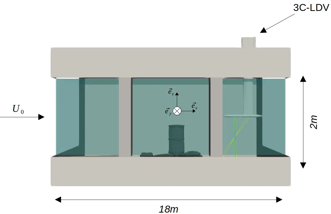
Tests are carried out in the Ifremer’s wave and current flume tank, located in Boulogne-sur-Mer in northern France. Extensively presented in [21], the tank experimental working section is 18 m long, 4 m wide and 2 m deep. The flow circulates in a loop controlled with a velocity range from 0.1 m·s−1 to 2.0 m·s−1 using two 250 kW pumps. The three-component flow velocity (U, V, W) is decomposed into the Cartesian coordinate system $$\left(\stackrel{\to }{{e}_{x}},\stackrel{\to }{{e}_{y}},\stackrel{\to }{{e}_{z}}\right)$$ represented in Figure 1. The x-axis denotes the longitudinal direction of the flow, and the origin is defined such that x = 0 m corresponds to the centre of the turbine (described in Section 2.2), y = 0 m is the median plan of the flume tank, and z = 0 m is the tank bottom.
A grid coupled to a honeycomb positioned at the inlet of the working section regulates the flow and the turbulence level. These flow straighteners allow the axial U component of the flow to remain constant throughout the height of the tank, thereby generating a uniform vertical velocity profile (named “Uniform condition”). Sheared velocity profiles are generated using two different “Panels”, each composed of several layers of wire mesh (Figure 2). This type of grid arrangement has already proved its worth in wind tunnel applications and has already been tested in tank experiments at ifremer’s wave and current flume tank [22,23]. The coarse mesh consists of 2 mm-thick wires spaced at 10 mm intervals, while the fine mesh consists of 0.7 mm-thick wires spaced at 2 mm intervals.
As indicated above, vertical velocity gradients are generated using wire mesh grids that vary according to the height of the water column. The 3 Components Laser Doppler Velocimetry (3C-LDV) probe in non-coincident mode is used to measure the incident velocity, as represented in Figure 1. The 3C-LDV system emits 3 pairs of laser beams of different wavelengths, all of which focus on a single point to provide a measurement volume of 0.01 mm3. For each pair, a laser beam crosses a bragg cell, creating a frequency shift between the two beams of each pair. At the crossing point of the laser beams, the difference in frequency between each pair generated by the Bragg cell produces interference fringes which, when a reflecting particle crosses this interfrange network, reflect the light wave at a specific frequency that can be measured. The particles injected to determine flow velocity are 10 µm silver-coated glass. The description of the LDV operating principle shows that the measurement sampling frequency depends on the number of particles crossing the measurement volume and varies between measurement points, ranging from 10 Hz to 150 Hz.
 |
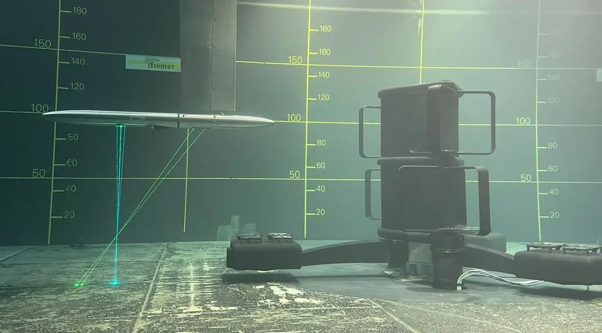 |
Figure 1. View of the flume tank test section with the coordinate system on the (left) and picture of the turbine model in the tank with the 3C-LDV on the (right).
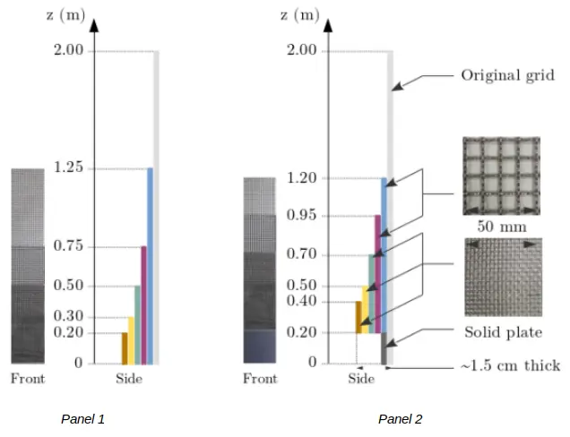
Figure 2. Panel 1 and 2 arrangements made up of several layers of wire mesh for sheared velocity profiles generation.
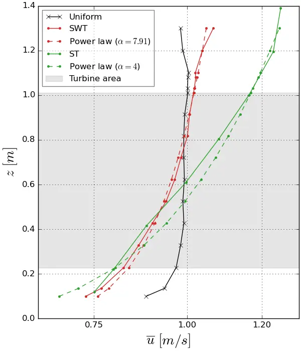
Figure 3a shows the profile of the time-averaged vertical velocity for the three cases. Two cases of sheared velocity profiles are studied, both assuming an average speed over the capture surface of the turbine close to the average velocity in uniform flow. The difference between the two shear velocity profiles is based on the turbulent intensity (TI) variation (Equation (1)), which varies according to the gradient considered. For the Panel 1 case, the turbulent intensity remains the same as for the uniform case. The turbine is therefore only subjected to a sheared flow known as “weakly turbulent” and will be referred to in the rest of the study by the abbreviation SWT for “Sheared Weakly Turbulent”. In the case of Panel 2, the turbulent intensity varies across the turbine’s capture surface, peaking at 7% at the bottom. This configuration will be abbreviated as ST for “Sheared Turbulent”.
where $$^{—}$$ $$\overline{}$$ is the average of the velocities, and σ is the classical standard deviation.
Often used by oceanographers, velocity profiles are commonly described using power laws [24,25,26], according to the following Equation (2), where 1/α is the Hellmann’s power law coefficient, Uref and zref are the reference velocity and height taken at the mid-depth of the water column.
For the SWT configuration, Hellmann’s power law coefficient gives a value of 7.91 and for the ST case, a value of 4. These values are within the range of values that can be found in situ [27] and indicate that the ST case presents a higher profile curvature than the SWT case. At sea, these power law coefficients are proportional to the tidal current velocity and are influenced by topographic conditions, such as rapid changes in seabed gradient at the bottom.
 |
 |
| (a) | (b) |
Figure 3. Mean streamwise velocity and turbulence intensity vertical profiles for the three conditions. (a) Streamwise velocity profiles; (b) Turbulence intensity.
In addition, the integral time scales for the three tested configurations are computed. According to [28,29], the integral time scale Lt is computed by integrating the temporal autocorrelation function Ruu(τ) over the time intervals from τ = 0 to the first zero crossing of Ruu(τ), Ruu(τ) = 0 corresponds to the limit beyond which fluctuations are no longer correlated, meaning that this threshold allows non-physical contributions such as noise to be excluded. Lt is defined by:
where:
Table 1 summarises all the characteristics of the flows imposed in the tank, averaged over the turbine’s capture surface, denoted by $$\hat{{\overline{\square}}}$$. The integral time scale has a value close to 1 under uniform flow conditions due to a good correlation of the velocity fluctuations measurements for two different times. The presence of a sheared flow introduces another dynamic. Uniform conditions result in a short integral time scale, which implies a more pronounced instability of the coherent structures that break down rapidly. Due to the heigth LDV frequency rate for these measurements (>50 Hz), all the flow characteristics given in Table 1 have an uncertainty lower of 2%.
Table 1. Sheared velocity profiles characteristics.
| Cases | $$\bm{\hat{\overline{U_0}}[\mathrm{m} \cdot \mathrm{s}^{-1}]}$$ | $$\bm{\hat{\overline{T I}}[\%]}$$ | $$\bm{\hat{\overline{L_t}}[s]}$$ |
|---|---|---|---|
| Uniform | 0.99 | 2.05 | 0.98 |
| SWT | 0.93 | 2.20 | 0.56 |
| ST | 0.99 | 4.63 | 0.45 |
2.2. Turbine Model and Wake Measurements
The model studied is the 2.5 MW rated-power machine developed within the framework of the “FloWatt” farm project, carried out by the company HydroQuest, and planned to be deployed for the Alderney Race site (Figure 4) at a scale of 1/20. The model is made of two rotor columns, with each column being composed of two rotors divided into two stages. For each column, the two rotors have a 60° phase shift to avoid self-starting difficulties and to attenuate significant torque variations [30]. Each rotor consists of 3 (N) identical blades with a NACA0022 profile. The model was designed to maintain geometric similarity in the flume and thus respect the relationship between the heights of the turbine and the water column. The Froude similarity is then respected, and the Reynolds number is roughly 100 times lower than at full scale, but sufficient enough to be in a turbulent flow regime. The device has a total height (Hmodel) of 1.01 m and a width (Wmodel) of approximately 1.27 m. The blockage ratio is then approximately 16%. More specifically, the rotor radius R is 0.235 m, the blade height (hb) is 0.315 m, and the chord profile (c) is 0.063 m, giving the rotor an aspect ratio (R/hb) of approximately 1.34 and a solidity (s = Nc/2πR) of 0.13. The turbine height (ht), defined as being the height between the bottom and the top horizontal plates is: 0.720 m. The reference surface, representing the capture surface projection, is then:
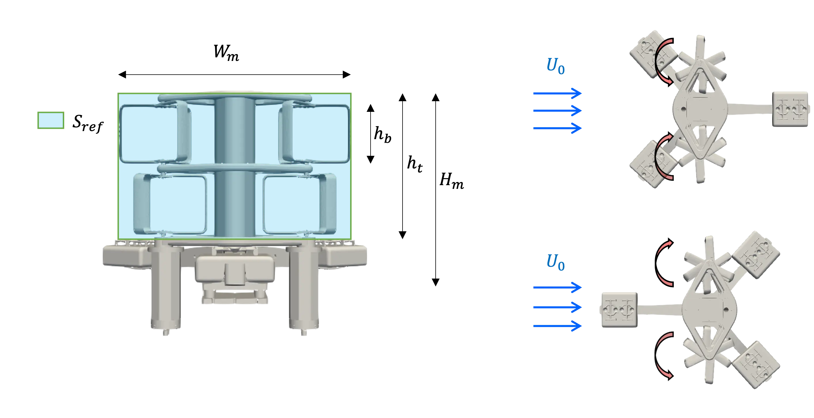
Figure 4. Schematic view of the model with its geometrical properties and the relative directions of rotation of the counter-rotating rotor columns.
In the same perspective, and to make it easier to compare with circular section technologies, an equivalent diameter (De) defined in the IEC (International Electrotechnical Commission) standards can be specified as follows:
The top view of the model shows a particular geometry of the baseplate, with three weighted arms arranged like a ‘tripod’. This base is connected to the lower horizontal plate of the turbine using a six component load cell. Based on the direction of rotation of the columns and the geometry of the baseplate, two configurations can be defined to simulate two flow directions. In the first case, the current first sees two base plates and rotor columns rotate so that, at the level of the central strut, the two counter-rotating rotor columns suck the fluid (Configurations “Co-Flow”). In the second case, the current first encounters a single base plate, and the two counter-rotating rotor columns push the fluid back (Configuration “Counter-Flow”). Throughout this study, only the “Counter-Flow” configuration is presented in both the performance and wake sections.
The turbine is equipped with two watertight blocks under each column to house the electronic and transmission systems. Each column is equipped with a Maxon RE50 DC motor, a speed encoder and a 1/26 speed reducer. A Scaime torquemeter (DR2112−W) and an angular position encoder are also incorporated in each block. The turbine is speed-controlled using remote Escon 70/10 servo-controllers. A National Instruments PXI system and LabView software are used to record each column’s angular speed (ωrot) and torque (Qcol), as well as the forces acting on the turbine model. The measurements are taken over a wide range of rotational speeds, subsequently specified by the advance parameter (λ) as the blade tip speed ratio. Each acquisition lasted 3 min with a sampling frequency of 512 Hz.
The mean power coefficient (Cp) and drag coefficient (Cx) are plotted as functions of λ, which is specified in Equation (7) [31]:
Fx represents the longitudinal load of the turbine as measured by a load cell included in the model’s baseplate and $$\hat{{\overline{{U}_{0}}}}$$ is the average of the velocities throughout the capture surface of the model. ρ denotes the water density.
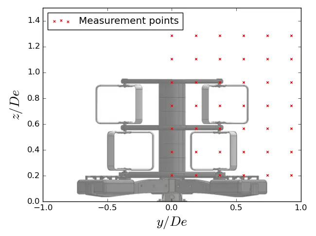
Besides, the downstream flow is measured using the 3C-LDV in non-coincident mode. The mesh, followed by the LDV probe, is represented in Figure 5. Assuming symmetry of the flow in the (y, z) plane, only half the width of the turbine was considered for these measurements (this assumption being previously checked [31]). The measurement planes in the (y, z) reference frame are repeated for several distances downstream from the turbine, ranging from 1.5 De to 9.5 De for the uniform and SWT configurations (see Figure 5b) and only from 1.5 De to 7.5 De for the ST case. The acquisition time for a measurement point is 3 min to guarantee signal convergence. The wake maps presented afterwards are the result of linear interpolation between mesh points. Experience from numerous test campaigns has shown that a high-density measurement grid is unnecessary. Comparisons between spatially high-resolution PIV measurements and temporally high-resolution LDV measurements [31,32] have proven that the measurement grid used in this study is sufficient to characterise wakes exhibiting relatively low velocity gradients between measurement points. To consider the vertical sheared velocity profile, the velocity measurements performed in the turbine’s wake are normalised by the reference velocity at the height considered.
 |
|
(a) |
 |
|
(b) |
Figure 5. C-LDV measurement point locations used for the three configurations (6 × 6 × 7 points of measurement in total). (a) Measurement points in the (y, z) plane (6 × 7 points); (b) Measurement points in the (x, z) plane (6 × 7 points).
3. Vertical Velocity Profile Effect on Performance
3.1. Average Performance Coefficient Assessment and Torque Distribution
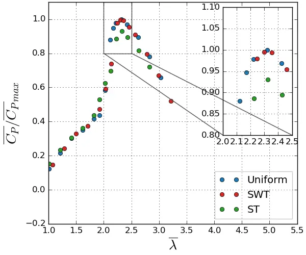
Figure 6a displays the time-averaged power coefficient with regard to λ for vertical sheared profiles compared to steady-state measurements. In all three study cases, the average power increases and then decreases, forming a bell shape curve and reaching a maximum at λ = 2.2. Using the uniform reference case’s greatest power coefficient to normalise the curves, the average performance shows a good match between the SWT and uniform cases. The presence of a weakly turbulent shear, therefore, does not impact the overall behaviour of the turbine. By coupling the sheared profile with turbulence, a decrease of about 7% is noted in the ST case compared to the uniform flow. This result is also obtained in [33] for a horizontal axis device. Figure 6b shows that the drag coefficient remains nearly unchanged by the presence of a vertical sheared profile even when coupled with turbulence. The slight variations observed between the sheared flows and the uniform reference case are not significant from the author’s point of view and can be attributed to the adimensionalisation process. Linant et al. [34] have already shown that the sheared flow is responsible for asymmetric loading between the upper and lower rotors, with the lower rotor producing less torque and reducing turbine performance.
 |
 |
| (a) | (b) |
Figure 6. Average turbine performance evolution as regard to the tip speed ratio. (a) Power coefficient; (b) Drag coefficient.
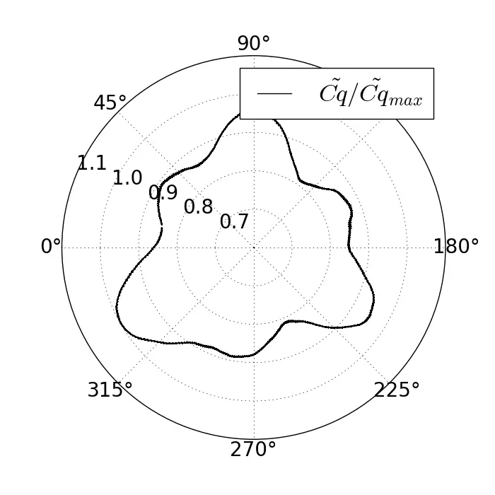
To go further, a comparison of the angular distribution of the torque coefficient (CQ, Equation (8)) of one of the rotor columns is also analysed. Since the instantaneous angular position is calculated and not measured.
The normalised phase-averaged torque distribution at λ = 2.2 for the three flow conditions represented in Figure 7 follows a relative angular distribution. A notable difference appears in the shape of the torque distributions. In uniform flow, six torque peaks phase-shifted by 60° are generated and correspond to the six blade passages that compose the rotor column as obtained during the study of a similar-looking ducted vertical double-axis tidal turbine [13]. The asymmetry of the flow along the vertical axis makes torque production challenging and is manifested by the presence of only 3 torque peaks, indicating an uneven distribution among each rotor constituting the column.
According to the author’s point of view, in the case of SWT, due to the dependence on the rotor columns rotational velocity, the lower rotors rotate at excessively high speeds relative to the perceived average incident flow, which promotes performance losses related to viscous friction. On the contrary, the top rotors perceive a nearly uniform incident velocity slightly above 1 m/s, thereby producing greater torque and reducing the performance gap with the uniform reference case. On the contrary, in the ST case, the top rotors rotate at too low speeds and the bottom rotors at too high speeds relative to the perceived average flow, which gives the turbine both stall effects on the upper rotors and viscous effects on the lower rotors. The turbulent intensity is also playing a role, and these combined effects reduce column torque production by about 12% compared to the uniform case.
 |
 |
 |
| (a) | (b) | (c) |
Figure 7. Normalised phase-averaged torque distribution at λ = 2.2 for the three flow conditions. Torque distributions are normalised by the maximal phase-average torque, measured in the uniform flow reference. (a) Uniform flow; (b) SWT flow; (c) ST flow.
3.2. Flow Effect in the Frequency Domain
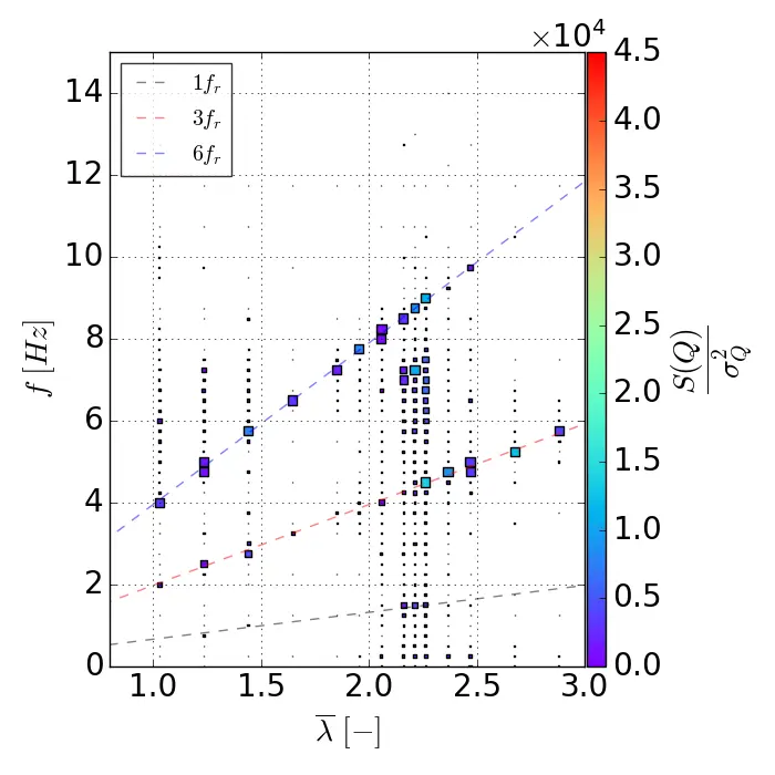
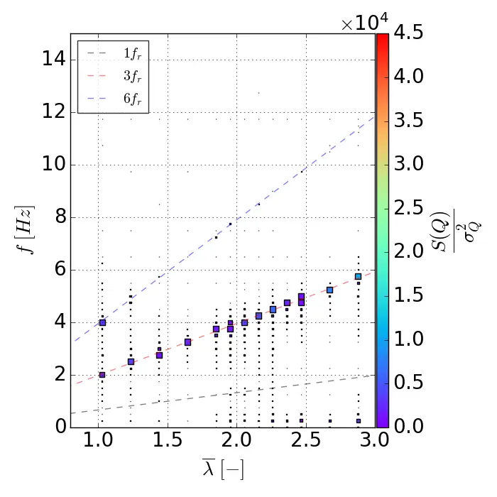
To study the effect of the vertical velocity profile in the frequency domain, a spectral analysis of the torque fluctuations of a rotor column is performed using the Campbell diagram shown in Figure 8. The diagram is employed to visualise the eigenfrequencies related to the dynamics of the rotor columns and to identify the resonance modes.
 |
 |
 |
| (a) | (b) | (c) |
Figure 8. Campbell diagrams for the three flow conditions. (a) Uniform flow; (b) SWT flow; (c) ST flow.
Only the uniform flow and the SWT cases show a response to the third harmonic of the rotational frequency (6 fr) while the ST case only shows a response at 3 fr across all rotational speeds, again demonstrating the disparity that can exist between the lower and the upper rotors and confirming the presence of only three torque peaks in the Figure 7c. It is quite interesting to note that in the uniform and SWT cases, the torque response at 6 fr is predominant for 1.0 < λ < λopt and that a transition between 6 fr and 3 fr occurs around λopt to then only give a torque response at 3 fr for the higher λ. The presence of the velocity sheared in the SWT case induces a stronger torque response at (3 fr), also explaining why the phase-averaged torque distribution shows 3 torque peaks in the SWT case compared to 6 for the uniform case (see Figure 7). While average performance is hardly affected, instantaneous torque production is significantly affected by the velocity profile. A sheared flow causes an asymmetry in production between the lower and upper rotor stages and has harmful consequences, such as reducing the turbine’s lifetime. The impact of these effects on the behavior of the turbine wake is studied in the following section in order to investigate how mechanical behavior influences the hydrodynamic behavior.
4. Vertical Velocity Effect on the Wake Behaviour
In this section, the effect of a sheared velocity profile on the turbine’s wake development is studied for a single rotational speed corresponding to the turbine’s optimal operating point, i.e., λ = 2.2.
4.1. Average and Fluctuating Wake Results
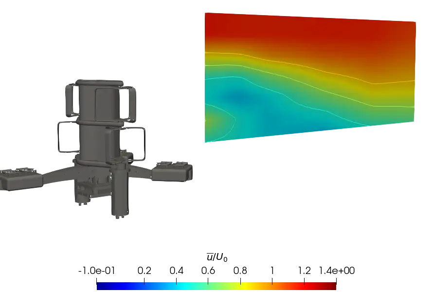
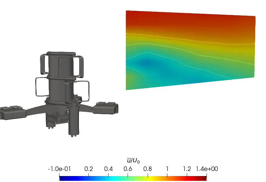
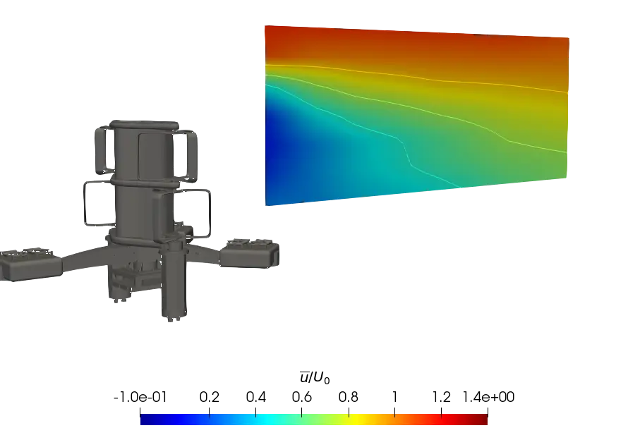
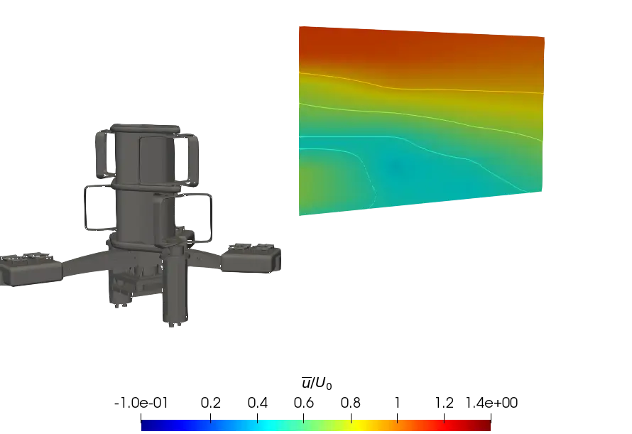
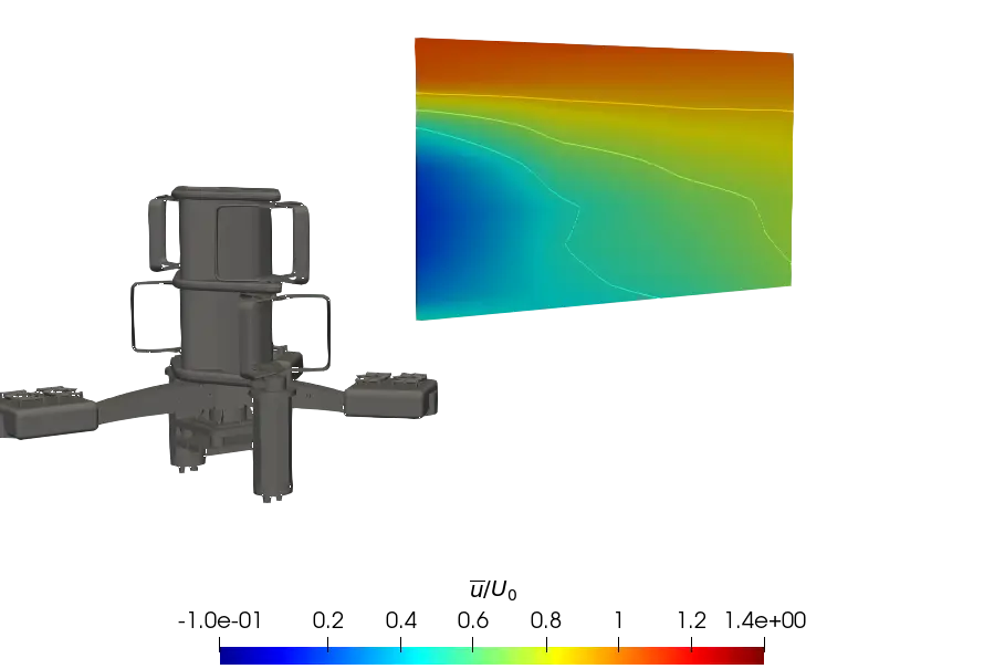
In order to give a global point of view, Figure 9 presents the contours of the time averaged streamwise velocity measured in the (x, z) plane of the turbine wake in the central strut plane (Figure 9a,c,e) and in the mid-rotor plane (Figure 9b,d,f). Overall, the results clearly show a more pronounced velocity deficit recovery, with the velocity profile exhibiting a higher rate of turbulent intensity. Comparison of the SWT and uniform cases shows that wake development is similar between the two configurations, for both planes. Thus, the faster recovery of the wake in the ST case is assumed to be induced by the turbulent rate of the flow, which is responsible for better mixing between the ambient flow and the flow in the wake due to the destruction and deformation of swirl structures, as it can be found in the literature [35]. In the far wake of the turbine, the wake boundary delimited by the yellow contour u/U0 = 0.9 in the figures is significantly higher in the sheared flows, and this is even more pronounced in the ST case.
 |
 |
|
(a) |
(b) |
 |
 |
|
(c) |
(d) |
 |
 |
|
(e) |
(f) |
Figure 9. Contours of the normalised average streamwise velocity at λ = 2.2 in (x, z) planes at the central strut and mid-rotor lateral positions. (a) Central strut plane for uniform flow; (b) Mid-rotor plane for uniform flow; (c) Central strut plane for SWT flow; (d) Mid-rotor plane for SWT flow; (e) Central strut plane for ST flow; (f) Mid-rotor plane for ST flow.
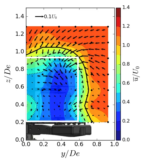
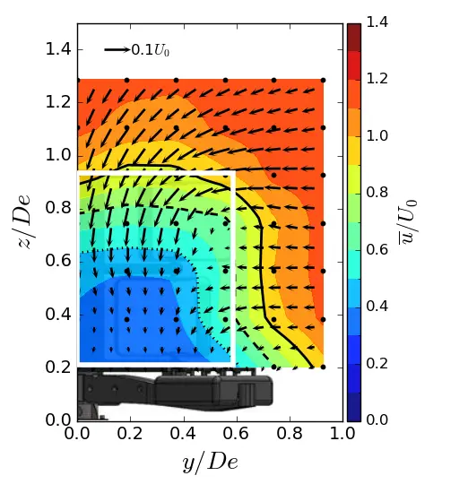
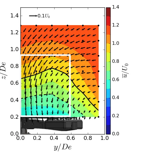
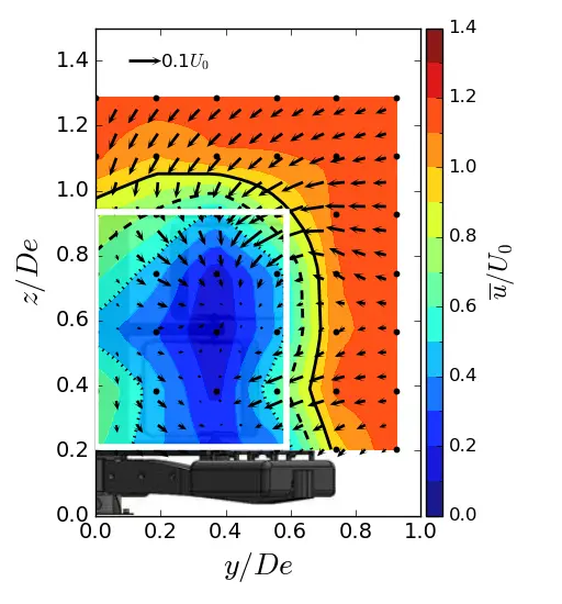
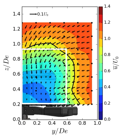
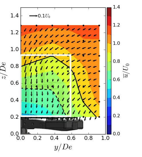
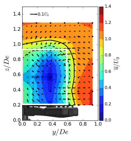
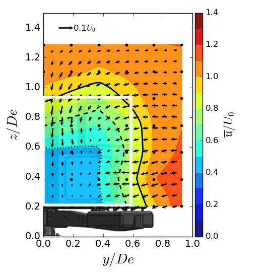
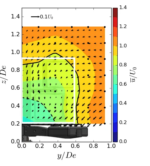
Figure 10, Figure 11 and Figure 12 show the contours of the time averaged velocity in the streamwise direction in the (y, z) planes for the different inflow conditions and for three downstream positions. Initially, near the turbine (at x/De = 1.5). For all these figures, the vectors superimposed are cross-stream and vertical velocities (v, w), and the white rectangle is the projected apparent capture area of the turbine. The three flow conditions exhibit a similar wake pattern with a wake boundary covering the turbine surface. Differences only appear at x/De = 3.5 and above. For uniform flow and SWT, the results show that the wake boundary gradually decreases in height until it equals or is smaller than the height of the turbine, and extends across the width. However, in the ST case, the wake contracts laterally and evolves little vertically, so that at 7.5 De, the average wake covers an area equivalent to that of the turbine.
In addition, the flow dynamics are highlighted by the superimposed vectors. The vector field allows us to visualise the exchange of momentum that occurs between the surrounding environment and the internal flow within the wake. At x/De = 1.5, a vortex dynamic is observed on the top corner of the tidal turbine for the three flow regimes. This swirling motion is well identified in the literature and corresponds to the vortex shedding at the blade tips undergone by vertical axis turbines. The strength of these swirls appears to be sensitive to the turbulent intensity rate imposed at the inlet, as observed by [36], since a smaller amplitude of swirls is observed in the ST case, while those in the uniform and SWT cases are of equal strength. Furthermore, the swirls appear to be more persistent downstream in the uniform case compared to the other cases. From the author’s point of view, these vortex structures are created to compensate for the velocity deficit and facilitate mixing between the wake and the free flow. However, the dissipation rate of these vortices is positively correlated with the wake recovery rate, such that a high wake recovery rate will result in faster dissipation of these structures. As can be seen, the velocity deficit is more pronounced at x/De = 3.5, where the profile is uniform, while it is sharply diminished in the other cases, which explains why the rotational dynamics can still be detected in the upper corner only in the uniform case.
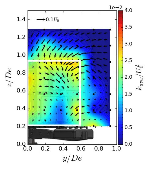
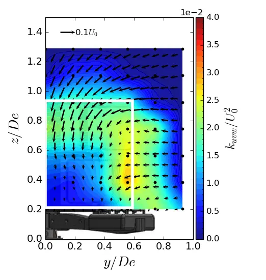
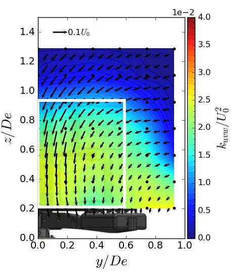
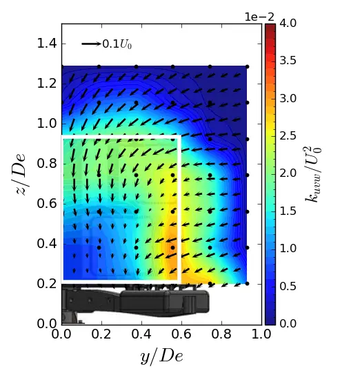
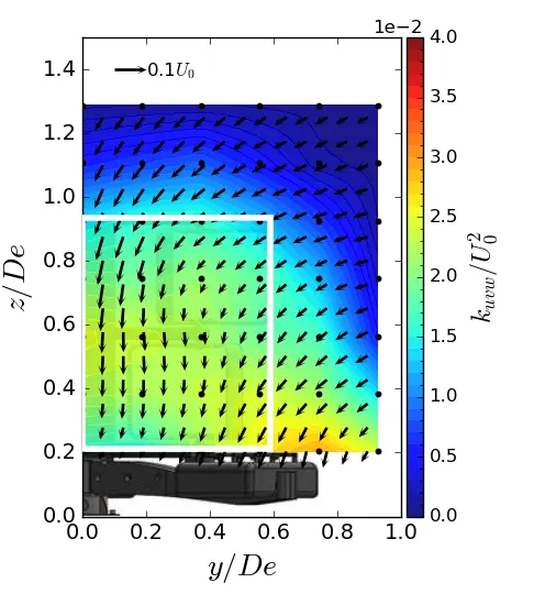
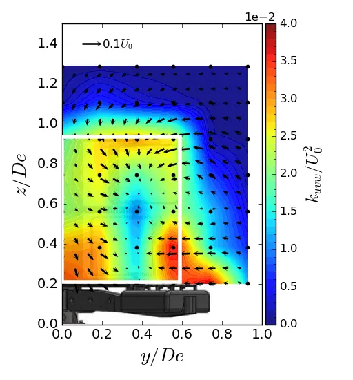
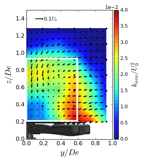
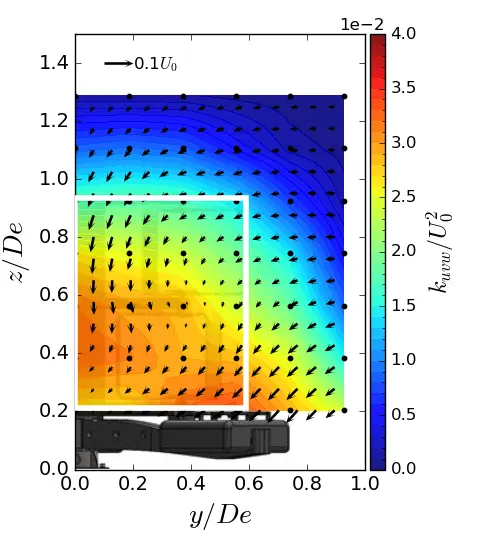
To supplement the analysis of the turbine wake dynamics, the normalised 3D turbulent kinetic energy (kuvw, Equation (9)) maps at 3 downstream positions in (y, z) planes are gathered in Figure 13, Figure 14 and Figure 15. The velocity vector field (v, w) is also represented.
 |
 |
 |
|
(a) |
(b) |
(c) |
Figure 10. Mean streamwise velocity in (y, z) planes in uniform flow condition. (a) x = 1.5 De; (b) x = 3.5 De; (c) x = 7.5 De. The white rectangle is the projected apparent capture area of the turbine and the black line is the u/U0 = 0.9 contour.
 |
 |
 |
|
(a) |
(b) |
(c) |
Figure 11. Mean streamwise velocity in (y, z) planes in SWT condition. (a) x = 1.5 De; (b) x = 3.5 De; (c) x = 7.5 De. The white rectangle is the projected apparent capture area of the turbine and the black line is the u/U0 = 0.9 contour.
 |
 |
 |
|
(a) |
(b) |
(c) |
Figure 12. Mean streamwise velocity in (y, z) planes in ST condition. (a) x = 1.5 De; (b) x = 3.5 De; (c) x = 7.5 De. The white rectangle is the projected apparent capture area of the turbine and the black line is the u/U0 = 0.9 contour.
In the near wake of the turbine (i.e., from x/De = 1.5 to 3.5), the high value of kuvw is concentrated on the y and z sides of the turbine’s capture area, as illustrated by the white rectangle in the maps. The main contributors to the high level of kuvw include the central strut wake, the blade tips, which are responsible for vortex shedding, and the feet of the gravity base, which constrain the flow. At x/De = 7.5, the turbulent kinetic energy is spread over the entire surface of the wake for all three flows. The only difference between the configurations lies in the magnitude level of kuvw. At x/De = 7.5, the ST case shows an increase of approximately 23% compared to the uniform flow. The SWT case shows an approximately 11% increase, indicating a lower energy dissipation rate when the sheared velocity profile is coupled with a high turbulent intensity.
 |
 |
 |
|
(a) |
(b) |
(c) |
Figure 13. Turbulent kinetic energy contours in (y, z) planes in uniform flow condition. (a) x = 1.5 De; (b) x = 3.5 De; (c) x = 7.5 De. The white rectangle is the projected apparent capture area of the turbine.
 |
 |
 |
|
(a) |
(b) |
(c) |
Figure 14. Turbulent kinetic energy contours in (y, z) planes in SWT condition. (a) x = 1.5 De; (b) x = 3.5 De; (c) x = 7.5 De. The white rectangle is the projected apparent capture area of the turbine.
 |
 |
 |
|
(a) |
(b) |
(c) |
Figure 15. Turbulent kinetic energy contours in (y, z) planes in ST condition. (a) x = 1.5 De; (b) x = 3.5 De; (c) x = 7.5 De. The white rectangle is the projected apparent capture area of the turbine.
4.2. Spectral Content of the Wake
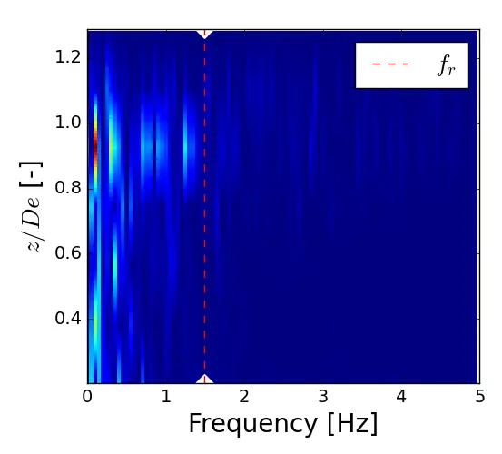
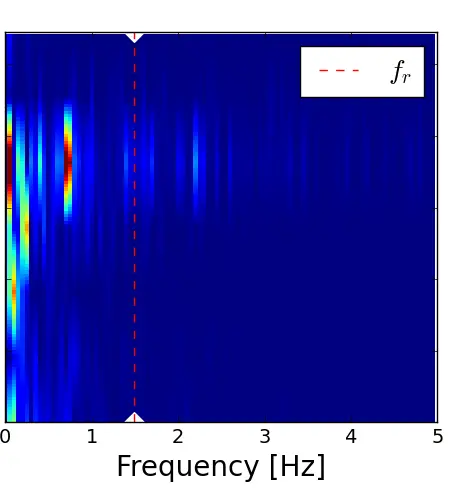
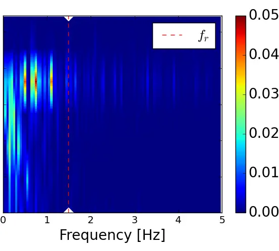
The distribution of the streamwise velocity fluctuations u′ in the frequential domain is represented in Figure 16 through PSD maps of u′ as a function of z/De, in the near wake of the model (x/De = 1.5) at position y/De corresponding to the middle of the model’s rotor column. For the three velocity profiles, PSD maps reveal a high energy density for frequencies between 0 and 1 Hz. The high energy density is mainly located at the apex of the turbine at the upper rotor (0.8< z/De < 1.0), as shown previously on the turbulent kinetic energy maps, where energy is concentrated on the y and z sides of the turbine’s capture area. The sheared velocity profiles reveal a higher spectral density compared to the uniform flow. However, no flow conditions show the signature of the turbine in the wake, since no harmonic of the rotational frequency stands out with high energy density. According to the author, this can be attributed to the distance x/De = 1.5, at which the maps are made, being too far away to detect frequencies related to the turbine. Thus, due to the lack of measurements in the very close wake of the turbine, it is difficult to compare the hydrodynamic effects with the mechanical effects.
 |
 |
 |
|
(a) |
(b) |
(c) |
Figure 16. Spectral power density maps of u′ at x/De = 1.5 and y/De = 0.56 for the three flow conditions. (a) x = 1.5 De; (b) x = 3.5 De; (c) x = 7.5 De.
4.3. Sheared Effect on the Wake Recovery
By applying the Taylor-Young formula of order 1 to the contour u/U0 = 0.9, it is possible to extract the coordinates z/De and y/De of the contour. The average of these coordinates allows us to evaluate the evolution of the average height and width of the wake in relation to the downstream position. The average wake height is calculated over the half width of the turbine (0.00 < y/De < L/2De), as indicated by the red dots and the average wake width is calculated between the middle of the lower rotor and the middle of the upper rotor, as shown by the blue dots (see Figure 17).
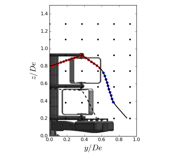
Figure 17. Example of the coordinates used to calculate the average height and width of the wake at x/De = 7.5 in SWT. Blue dots = y/De and red dots = z/De.
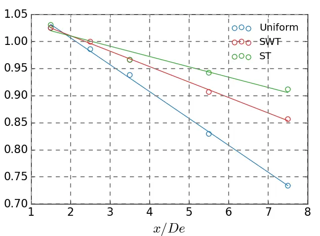
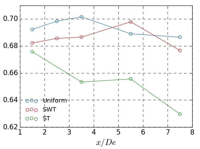
The average wake height is presented in Figure 18a. It shows that the wake height decreases gradually with downstream distance across the three flow conditions. Close to the turbine (at x/De = 1.5), the results suggest that the width of the wake remains unchanged regardless of the flow considered. From x = 2.5 De to x = 3.5 De, a first distinction can be made between shear flows, presenting similar widths, and uniform flow, which reveals a weaker width than the other two cases. The uniform case shows a lower width in the far wake with a faster decay. The drop observed from x/De = 1.5 to x/De = 7.5 in the uniform case is around 30%, while it is about 17% in SWT and 12% in ST. Figure 18b shows the average half wake width evolution with the downstream distance. The graph reveals that the wake width remains globally identical between the near wake (x/De = 1.5) and the far wake (x/De = 7.5) for the uniform and SWT profiles, with a magnitude y/De of the same order (y/De ≈ 0.68). In the opposite case, the ST flow decreases with the downstream distance to reach an average width of 0.63 at x/De = 7.5, which is 7% lower than the other two cases.
 |
 |
| (a) | (b) |
Figure 18. Evolution of the wake dimensions as a function of the downstream position. (a) average wake height and (b) average wake width of u/U0 = 0.9 as a function of the downstream positions.
Figure 19 represents the surface area of the wake by looking at its variations with regard to the equivalent diameters downstream of the turbine. It is important to note that the mesh is not sufficiently coarse to obtain the entire wake boundaries, particularly in the uniform case at x/De = 7.5, suggesting caution should be exercised with regard to the results provided and the analysis carried out. The overall trends of the curves reveal that between x/De = 1.5 and x/De = 7.5, the wake area decreases linearly with positions downstream of the turbine. The slope values indicate that the wake of the model in the presence of uniform flow decreases slightly faster than in cases with a sheared velocity profile. The SWT flow shows the largest wake area and appears to decrease at the same rate as the ST case. Beyond x/De = 7.5, the surface area of the wake, for uniform and SWT flows, remains constant.
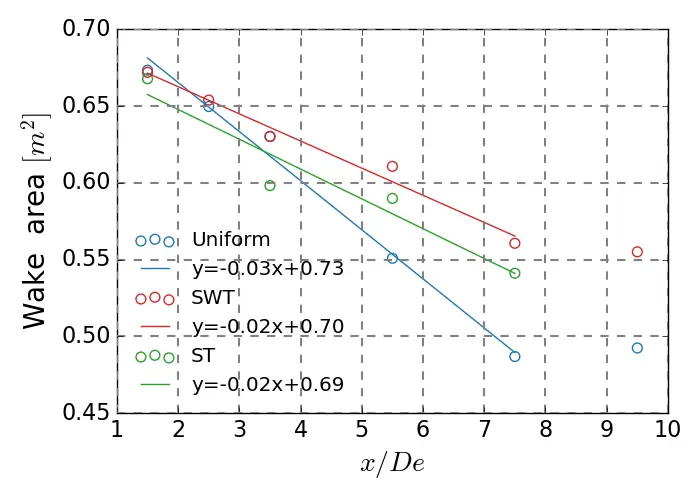
Figure 19. Evolution of the wake area as a function of the downstream position for the three test cases.
In the literature and especially on horizontal-axis technologies [37,38,39], the recovery of the velocity deficit in the wake is often described by using empirical power laws following the equation:
A simple, similar model was built to describe the development of the velocity deficit in vertical-axis turbines. Ref. [40] proposed an empirical model containing three coefficients such that:
By resuming the work of [40,41] showed that the recovery of the wake deficit could be predicted by knowing the maximum velocity deficit in the near-wake of the turbine. Thus, the coefficient c3 in Equation (11) becomes Umin according to the suggestion made by [41]. Using this approach, an estimation of the distance x/De at which the downstream flow recovers 90% of the incident flow rate could be made. In our case, the basic model (Equation (11)) was extended to examine the recovery of the surface-averaged streamwise velocity over the wake area where u/U0 = 0.9 to give Equation (12).
Figure 20 displays the evolution of the surface-averaged streamwise velocity over the wake area where u/U0 = 0.9, noted <u/U0>0.9, with the downstream distance for the three flow conditions. This metric allows us to compare the intensity of the velocity deficit in the wake of the turbine. The application of the curve fit model, defined in Equation (12), to the different flow cases shows that the model follows the experimental data quite well, with a coefficient of determination R2 > 0.95 for the three cases. Even though the ST case does not present data at x/De = 9.5, a preliminary estimate of the wake recovery length can be calculated. By adjusting the model with the correct coefficients c1 and c2, the results show that the ST case would be favorable for a faster recovery of the velocity deficit in the wake, with a recovery length at x/De ≈ 14 compared to x/De ≈ 17 and x/De ≈ 19 for the SWT and uniform cases, respectively. The coefficients employed in the model and the values of the recovery length are summarised in Table 2.
Table 2. Model coefficients and estimated recovery length.
|
Cases |
```latex{\bm{c}}_{1}``` |
```latex{\bm{c}}_{2}``` |
```latex\hat{ \overline{{\bm{L}}_{\bm{t}}}}\left[\mathbf{s}\right] \left[\mathbf{m}·{\mathbf{s}}^{-1}\right]``` |
```latex\bm{R}²``` |
```latex\bm{x}/\bm{D}\bm{e}``` |
|
Uniform |
0.592 |
0.201 |
0.178 |
0.98 |
19 |
|
SWT |
0.517 |
0.234 |
0.098 |
0.99 |
17 |
|
ST |
0.596 |
0.210 |
0.141 |
0.99 |
14 |
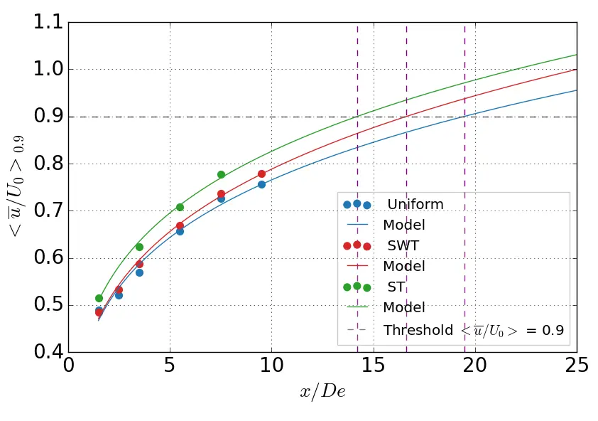
Figure 20. Surface averages of the streamwise velocity over the area where u/U0 < 0.9 with the model prediction in uniform, SWT and ST flow. The purple dashed lines are the crossover lines between the models, and the black dashed line is positioned at <u/U0>0.9.
4.4. Mean Momentum Transport Terms Contribution to the Wake Recovery
Following [32], the mechanisms of mean and turbulent transport related to wake recovery are studied using the Reynolds-averaged momentum equation in the streamwise direction (Equation (13)). The flow is assumed to be stationary on average and incompressible.
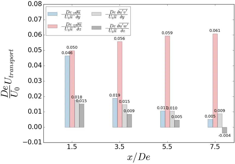
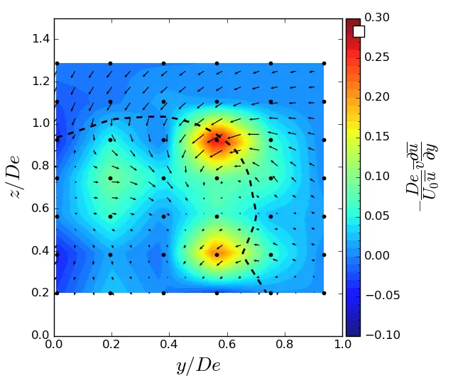
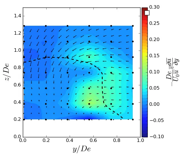
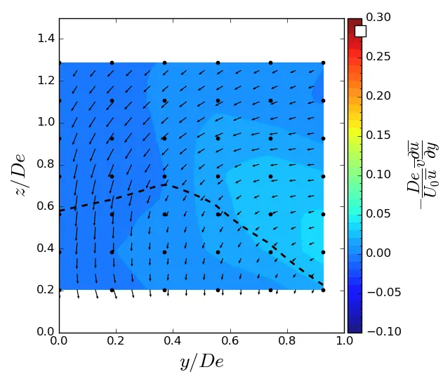
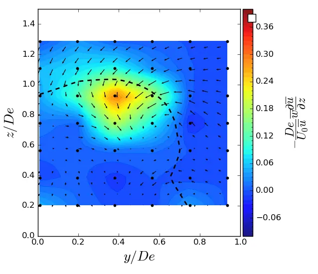
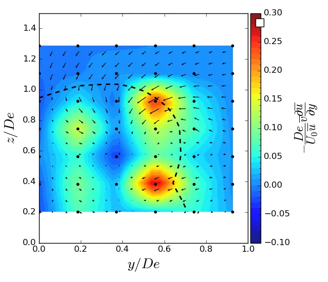
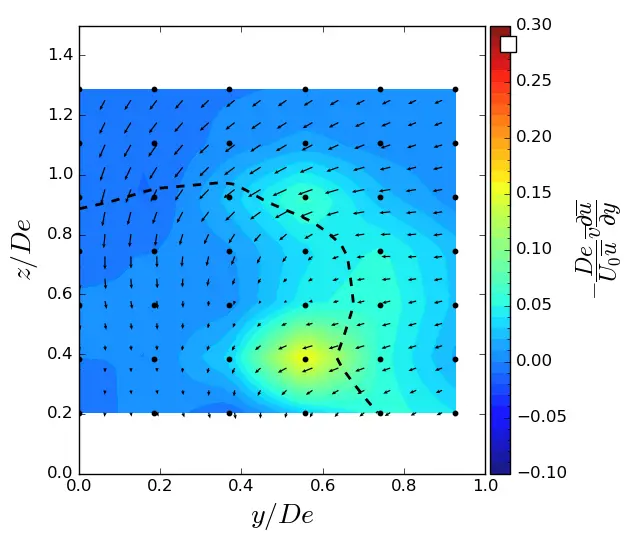
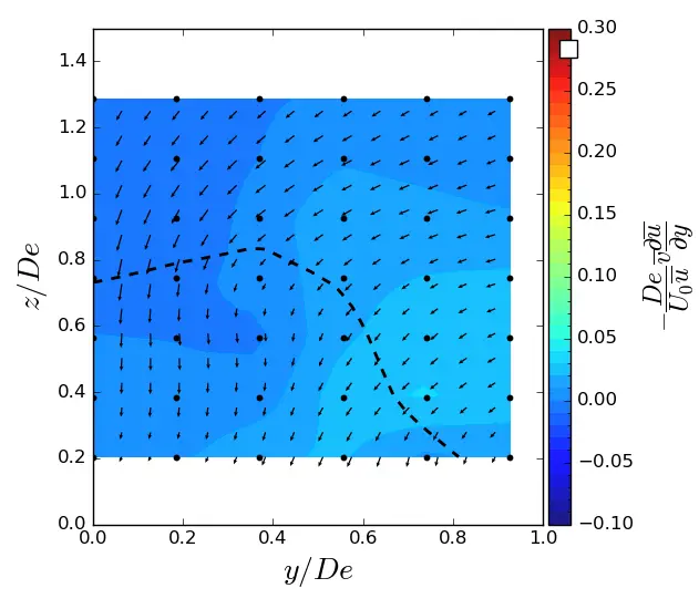
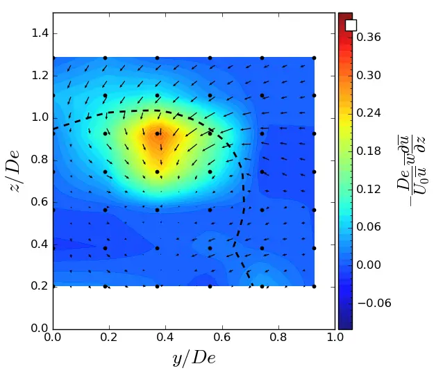
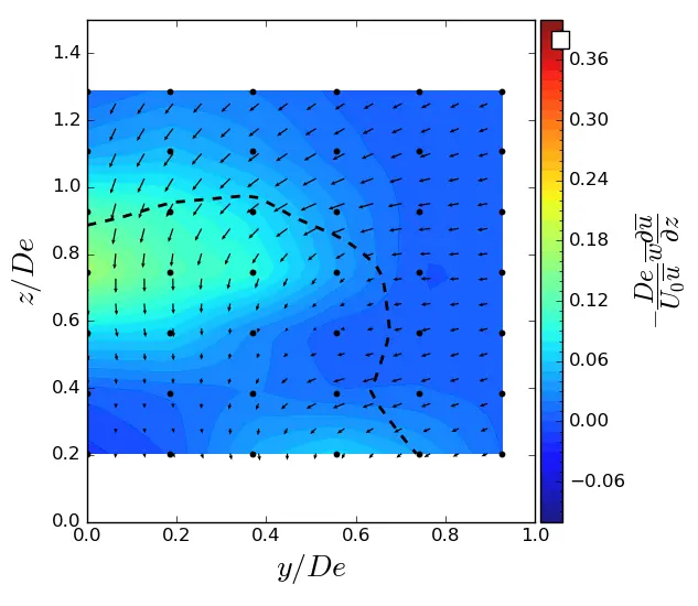
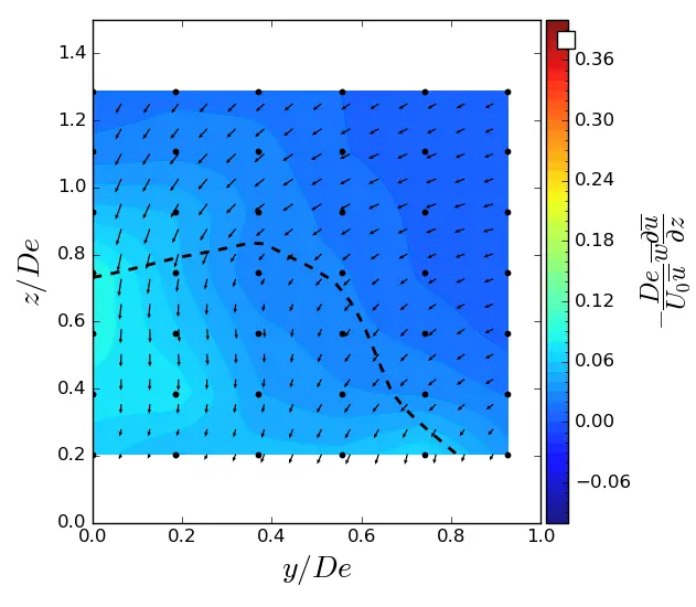
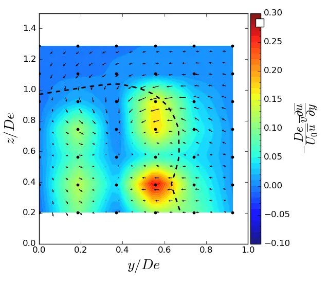
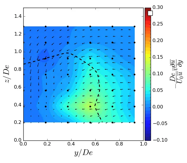
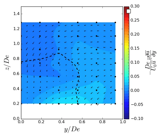
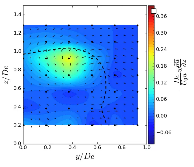
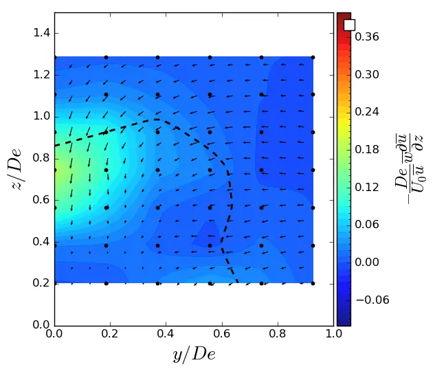
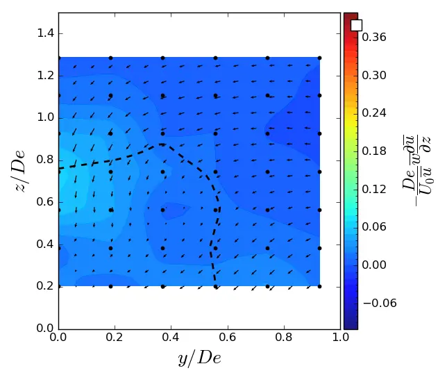
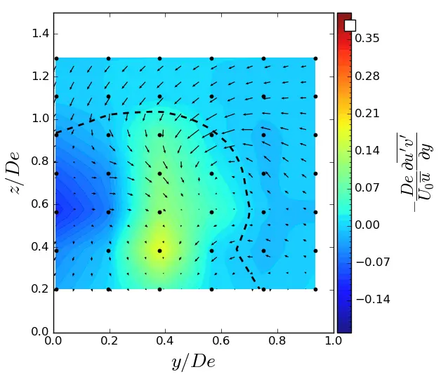
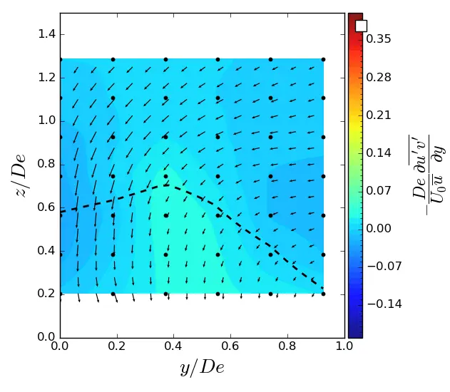
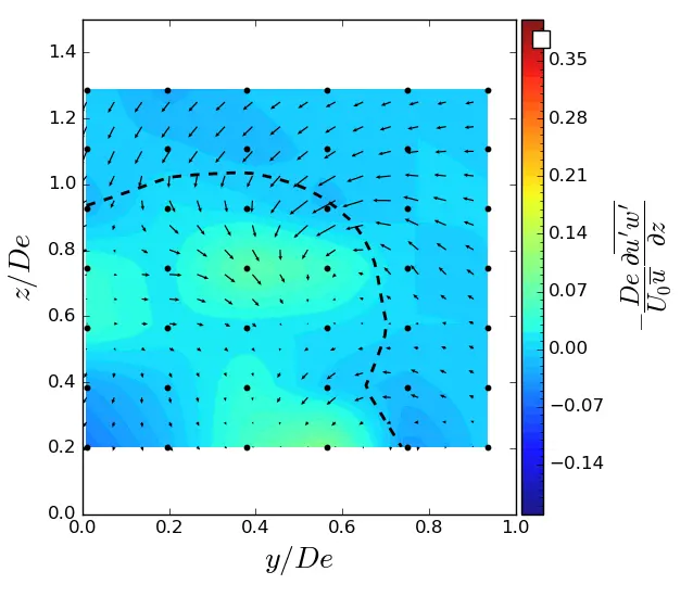
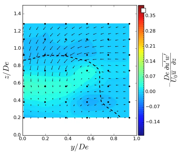
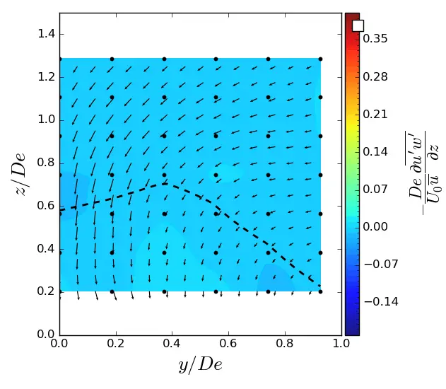
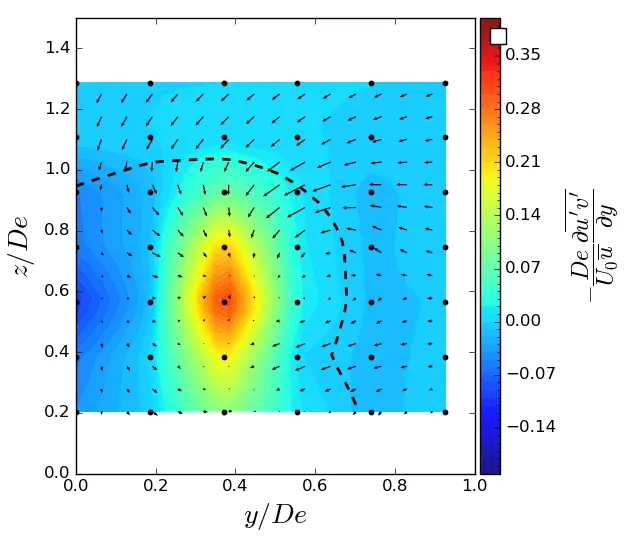
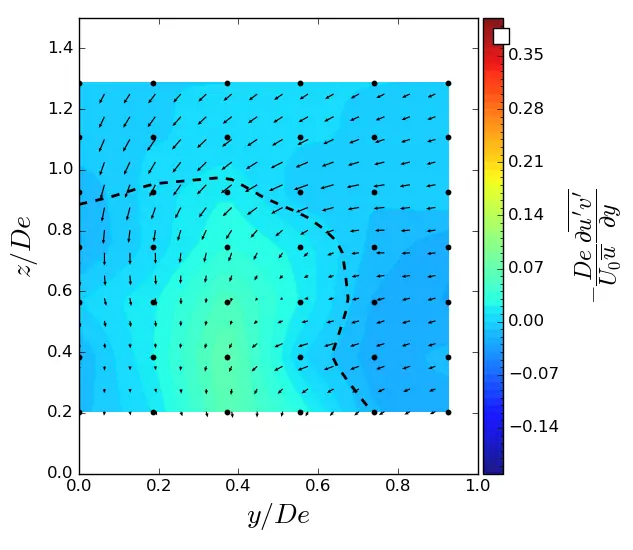
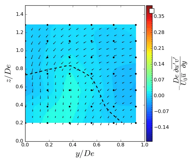
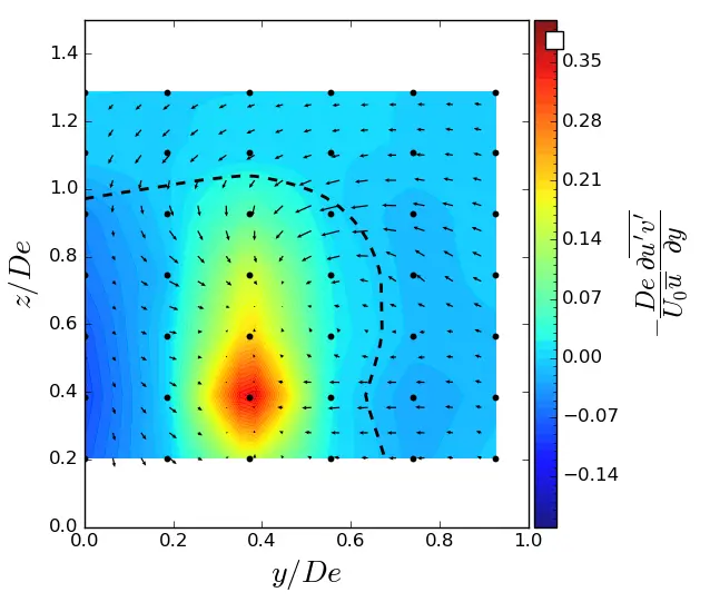
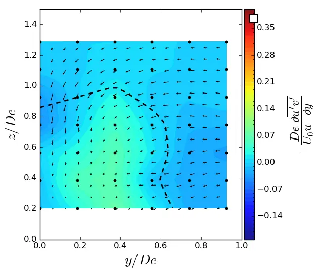
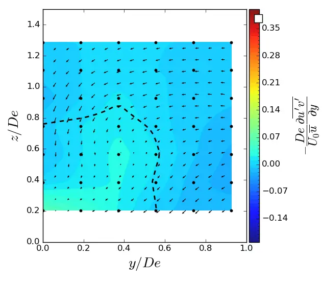
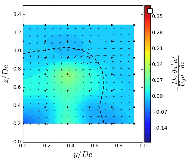
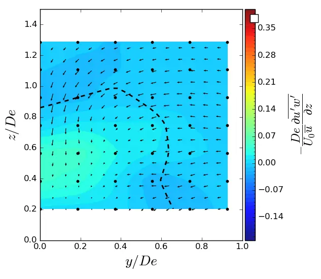
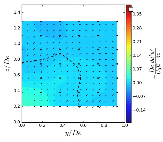
According to [41], based on the Reynolds number computed from the rotor diameter (ReD), the viscous effects are considered not significant for this study, so term VII is not calculated here. Finally, because the spatial discretisation along the longitudinal axis is too large, all the partial derivatives with respect to x shall not be presented here (i.e., terms III and IV are omitted). Terms I and II represent the average momentum transport along the y and z axes (also called y-advection and z-advection), and terms V and VI represent the turbulent momentum transport along the y and z axes (also called y-turbulent transport and z-turbulent transport). As performed in [32], the transport mechanisms of streamwise momentum are spatially averaged through the area bounded by the wake, i.e., for our study over the area where u/U0 < 0.9 and are presented in Figure 21 (the maps of average and turbulent contributions of the streamwise momentum are available in Appendixes A and B).
 |
|
(a) |
 |
|
(b) |
 |
|
(c) |
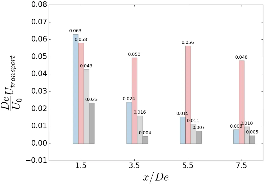
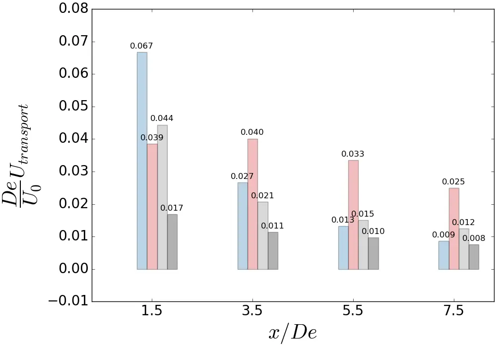
Figure 21. Bar plot of contributions to average momentum recovery in the longitudinal direction, spatially averaged over the area where <u/U0> = 0.9, normalised by the reference velocity and the equivalent diameter for the three flow cases. (a) Contribution repartition for uniform flow; (b) Contribution repartition for SWT flow; (c) Contribution repartition for ST flow.
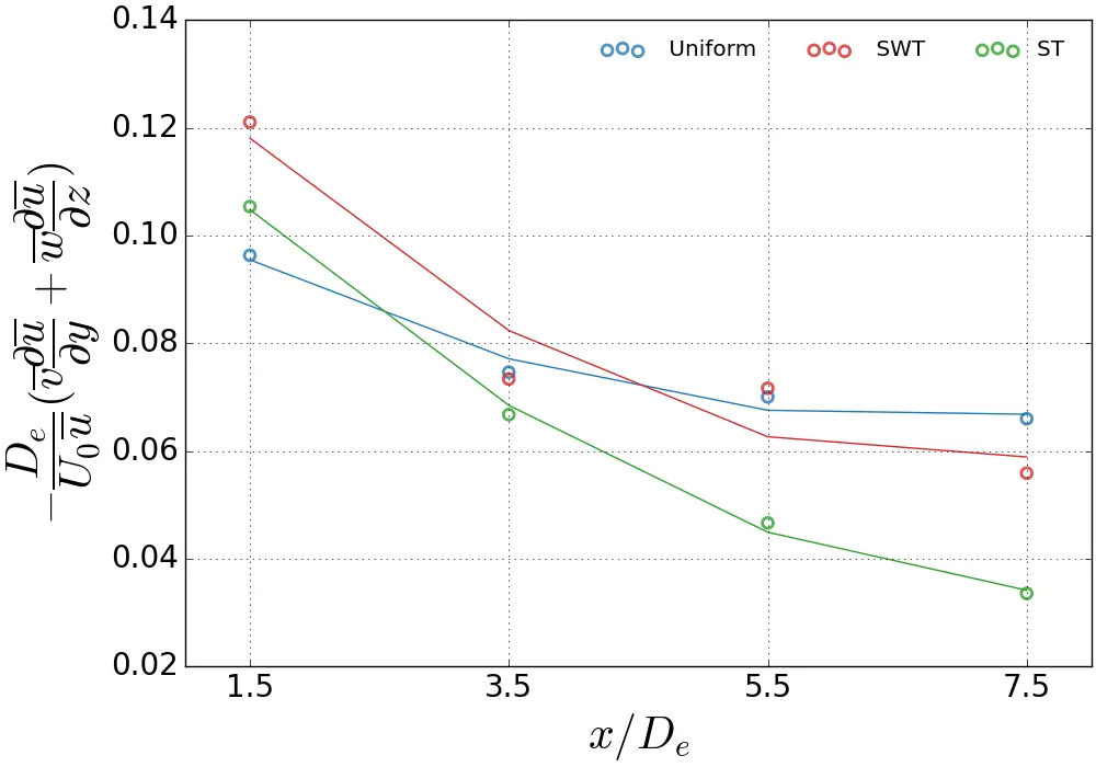
Derivatives were computed using second order central differences in the interior points and first order at the boundaries. Initially, at x/De = 1.5, the mechanisms responsible for the streamwise momentum recovery are the advection terms, with an identical contribution between the y-component and the z-component in the uniform and SWT cases. For x/De > 1.5, the mean momentum transport along the z-axis is the dominant component in wake recovery at further downstream distances and is attributed to tip vortices. For the ST flow, y-advection is first dominant at 1.5 De, followed by z-advection for the remaining lengths x/De. A decrease in z-advection is observed for the ST flow, resulting in values 2 to 3 times smaller in magnitude than in the uniform and SWT cases, thus explaining the differences in average wake heights mentioned in Section 4.3. Overall, the y-advection is identical in the ST flow and SWT cases, but slightly lower in the uniform case.
In addition, Figure 22 displays the total contribution of the average momentum transport by adding the y and z advections (Figure 22a) and the total contribution of the turbulent momentum transport by adding the y and z turbulent transports (Figure 22b) for each case. The contribution to the streamwise momentum recovery of the total average transport terms shown in Figure 22a reveals that turbulent intensity is responsible for a sharp decrease in advection terms. Indeed, at x/De = 7.5, the ST flow shows a magnitude almost twice as low as a uniform flow. However, with a low turbulent intensity rate, the SWT sheared velocity profile has the greatest amplitude in the near-wake of the turbine at x/De = 1.5, then approaches the uniform flow in values from 3.5 De onwards.
Figure 22b shows that at x/De = 1.5, the turbulent transport quantities are of the same order of magnitude between the sheared velocity profiles and are also more significant compared to the uniform case. Indeed, the turbulent terms are twice as significant with the sheared velocity profiles. For 3.5 < x/De < 7.5, the turbulent terms are slightly higher for ST than for SWT and the uniform flow. For 3.5 < x/De < 7.5, the turbulent terms are also slightly higher for ST than for SWT and uniform flow. It is noteworthy that at x/De = 7.5, the sum of the turbulent transport terms is of the same order of magnitude as the sum of the mean transport terms in the ST case, whereas for the other flow cases, the sum of the advection terms is dominant over all downstream distances. This phenomenon indicates a clear difference in wake recovery and explains why wake development differs across the flow cases, as shown previously in Section 4.1.
 |
 |
|
(a) |
(b) |
Figure 22. Evolution of the total contribution terms of streamwise momentum spatially averaged over the area where <u/U0> = 0.9 in the wake for the three flow cases. (a) Total average transport terms; (b) Total turbulent transport terms.
5. Conclusions
This work experimentally studies a vertical-axis tidal turbine operating in a sheared onset velocity profile, with two velocity profile cases identified by their level of turbulent intensity. When comparing the results to a uniform and stationary case, considered as ideal, the average performance of the tidal turbine is not directly impacted by the velocity profile but rather by the turbulence intensity rate, showing a slight drop in the power coefficient of 7% for the sheared velocity profile with the highest turbulence intensity rate. The trend of a slight decrease in the power coefficient in the presence of a sheared flow is consistent with studies carried out by [33,42] on a horizontal axis turbine. Nevertheless, studies indicate a significant impact of the velocity profile on local loads on rotor blades.
Although the average response of the turbine is almost identical between flow conditions, the angular distribution of the torque and its frequency response indicate a production asymmetry between the two rotors comprising a column of the model, with the presence of a sheared flow. As discussed in [19], which studies the effect of shear on a ducted quadrirotor vertical-axis tidal turbine in counter-rotating configuration, local measurements of the flow in front of the model show that, in the presence of a sheared velocity profile, the square of the velocity in front of the upper rotor is stronger than in front of the lower rotor, potentially indicating that the upper rotor produces most of the torque and thus explaining the appearance of only three peaks in the torque distribution and the predominance of 3 fr in the machine’s frequency response. The influence of the shear flow profile on the dominant frequency components in the torque response has also been highlighted by [43] for a two-bladed vertical axis wind turbine subjected to different atmospheric boundary layers.
The downstream flow development of the tidal turbine is also discussed in Section 4. The development of the wake shape depends on the inlet flow conditions, since non-uniform inlet flow conditions appear to result in a higher average wake height in the x/De positions furthest from the turbine, with a decrease of 30% for uniform flow and 17% and 12% for sheared flow without and with a high level of turbulence, respectively. However, the width of the wake is more sensitive to the level of turbulent intensity, since with no significant turbulent intensity, the sheared velocity profile has a slight impact on the average width of the wake. In contrast, the sheared velocity profile coupled with high turbulent intensity reduces the width of the wake when compared to the uniform profile.
An empirical law commonly used for horizontal axis technologies, which translates the evolution of the velocity deficit in the wake, is adapted to our model using a simple power law formula based on the minimum velocity in the near-wake of the turbine. The results reveal that the rate of velocity deficit recovery in the turbine wake increases when the inlet profile is sheared. Turbulence is responsible for better mixing in the wake, as the velocity profile with the highest turbulence intensity rate exhibits the fastest recovery. As highlighted by [44], which modelled the performance and near-wake development of a 25 kW four-bladed H-Darrieus vertical-axis tidal turbine in uniform flow and turbulent flow, the high turbulence intensity causes the vortices at the blade tip to interact at a distance closer to the turbine compared to low turbulence. This interaction distance is described as correlated with the position of the rapid recovery of the velocity deficit. The results provided by [44] are consistent with our study, since the evolution of transport terms shows a more rapid decrease in average transport terms, which can be attributed to the fast dissipation of vortices at the blade tip, in cases where the sheared velocity profile is coupled with a high turbulence rate.
In future work, the results presented here will need to be supplemented by additional tests in a uniform turbulent flow to distinguish the effect of turbulence and velocity profile on turbine performance and wake development. Furthermore, more accurate velocity measurements near the rotor column would be useful to better compare the mechanical behaviour of the turbine with its hydrodynamic characteristic, thereby supplementing the Section 4.2 dealing with the frequency components obtained in the wake of the model. As the current study focuses exclusively on the overall performance of the turbine, a lack of local load information must be taken into account for future tests in order to study the coherence between loads and wake variations. This work considers only a single operating point of the turbine. A more in-depth study, covering various operating conditions, should be conducted to evaluate the overall wake behavior for all operating points.
Appendix A
This appendix presents the contours of the average transport terms in the streamwise momentum balance equation for the three conditions.
 |
 |
 |
|
(a) |
(b) |
(c) |
Figure A1. y-advection in (y, z) planes in uniform condition. Vectors superimposed are cross-stream and vertical velocities (v, w). The dashed line represents the contour where <u/U0> = 0.9. (a) x = 1.5 De; (b) x = 3.5 De; (c) x = 7.5 De.
 |
 |
 |
|
(a) |
(b) |
(c) |
Figure A2. z-advection in (y, z) planes in uniform condition. Vectors superimposed are cross-stream and vertical velocities (v, w). The dashed line represents the contour where <u/U0> = 0.9. (a) x = 1.5 De; (b) x = 3.5 De; (c) x = 7.5 De.
 |
 |
 |
|
(a) |
(b) |
(c) |
Figure A3. y-advection in (y, z) planes in SWT condition. Vectors superimposed are cross-stream and vertical velocities (v, w). The dashed line represents the contour where <u/U0> = 0.9. (a) x = 1.5 De; (b) x = 3.5 De; (c) x = 7.5 De.
 |
 |
 |
|
(a) |
(b) |
(c) |
Figure A4. z-advection in (y, z) planes in SWT condition. Vectors superimposed are cross-stream and vertical velocities (v, w). The dashed line represents the contour where <u/U0> = 0.9. (a) x = 1.5 De; (b) x = 3.5 De; (c) x = 7.5 De.
 |
 |
 |
|
(a) |
(b) |
(c) |
Figure A5. y-advection in (y, z) planes in ST condition. Vectors superimposed are cross-stream and vertical velocities (v, w). The dashed line represents the contour where <u/U0> = 0.9. (a) x = 1.5 De; (b) x = 3.5 De; (c) x = 7.5 De.
 |
 |
 |
|
(a) |
(b) |
(c) |
Figure A6. z-advection in (y, z) planes in ST condition. Vectors superimposed are cross-stream and vertical velocities (v, w). The dashed line represents the contour where <u/U0> = 0.9. (a) x = 1.5 De; (b) x = 3.5 De; (c) x = 7.5 De.
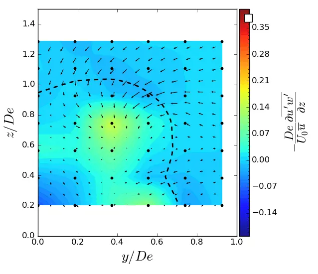
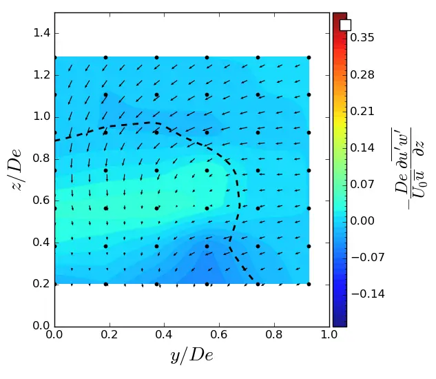
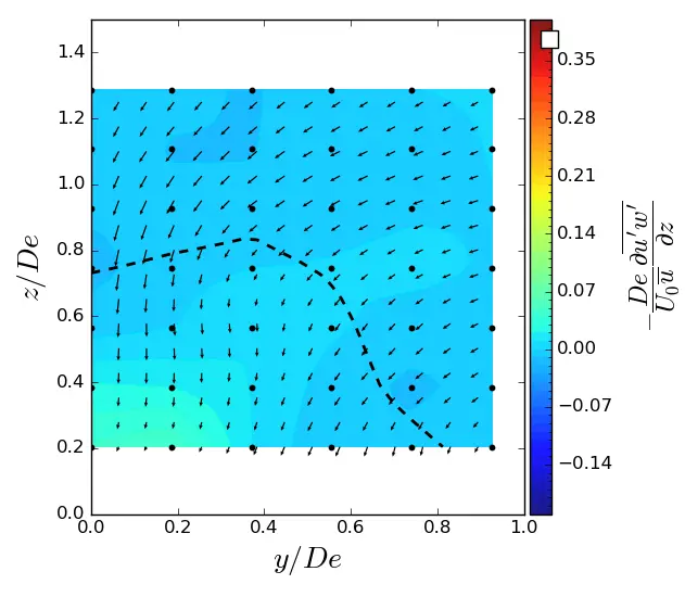
Appendix B
This appendix presents the contours of the turbulent transport terms in the streamwise momentum balance equation for the three conditions.
 |
 |
 |
|
(a) |
(b) |
(c) |
Figure A7. y-turbulent in (y, z) planes in uniform condition. Vectors superimposed are cross-stream and vertical velocities (v, w). The dashed line represents the contour where <u/U0> = 0.9. (a) x = 1.5 De; (b) x = 3.5 De; (c) x = 7.5 De.
 |
 |
 |
|
(a) |
(b) |
(c) |
Figure A8. z-turbulent in (y, z) planes in uniform condition. Vectors superimposed are cross-stream and vertical velocities (v, w). The dashed line represents the contour where <u/U0> = 0.9. (a) x = 1.5 De; (b) x = 3.5 De; (c) x = 7.5 De.
 |
 |
 |
|
(a) |
(b) |
(c) |
Figure A9. y-turbulent in (y, z) planes in SWT condition. Vectors superimposed are cross-stream and vertical velocities (v, w). The dashed line represents the contour where <u/U0> = 0.9. (a) x = 1.5 De; (b) x = 3.5 De; (c) x = 7.5 De.
 |
 |
 |
|
(a) |
(b) |
(c) |
Figure A10. z-turbulent in (y, z) planes in SWT condition. Vectors superimposed are cross-stream and vertical velocities (v, w). The dashed line represents the contour where <u/U0> = 0.9. (a) x = 1.5 De; (b) x = 3.5 De; (c) x = 7.5 De.
 |
 |
 |
|
(a) |
(b) |
(c) |
Figure A11. y-turbulent in (y, z) planes in ST condition. Vectors superimposed are cross-stream and vertical velocities(v, w). The dashed line represents the contour where <u/U0> = 0.9. (a) x = 1.5 De; (b) x = 3.5 De; (c) x = 7.5 De.
 |
 |
 |
|
(a) |
(b) |
(c) |
Figure A12. z-turbulent in (y, z) planes in ST condition. Vectors superimposed are cross-stream and vertical velocities (v, w). The dashed line represents the contour where <u/U0> = 0.9. (a) x = 1.5 De; (b) x = 3.5 De; (c) x = 7.5 De.
Acknowledgments
The authors acknowledge Benoit Gomez for his help during the tests and the data analysis.
Author Contributions
Conceptualization, R.L., G.G. and G.M.; Methodology, R.L., B.G., J.-V.F., C.P. and G.G.; Validation, R.L., Y.S. and B.G.; Formal Analysis, R.L.; Investigation, R.L., Y.S., J.-V.F. and G.G.; Data Curation, R.L.; Writing—Original Draft Preparation, R.L.; Writing—Review & Editing, R.L., Y.S. and G.G.; Visualization, R.L.; Supervision, C.P., G.G. and G.M.; Project Administration, G.G. and G.M.; Funding Acquisition, G.G. and G.M.
Ethics Statement
Not applicable.
Informed Consent Statement
Not applicable.
Data Availability Statement
The data supporting the findings of this study are available from the corresponding author, upon reasonable request.
Funding
This research was funded by the French Agence Nationale de la Recherche through the Verti-Lab project (ANR-23-LCV1-0009-01), the French Research and Technology National Association (ANRT) under the convention Cifre n◦ 2023/0217 and the CPER IDEAL.
Declaration of Competing Interest
The authors declare that they have potential conflicts of interest, some of them being employed by HydroQuest and all working together on the Verti-Lab project.
References
- Maka AOM, Ghalut T, Elsaye E. The pathway towards decarbonisation and net-zero emissions by 2050: The role of solar energy technology. Green Technol. Sustain. 2024, 2, 100107. doi:10.1016/j.grets.2024.100107. [Google Scholar]
- Copping A, Wood D, Rumes B, Ong EZ, Golmen L, Mulholland R, et al. Effects and management implications of emerging marine renewable energy technologies. Ocean Coast. Manag. 2025, 264, 107598. doi:10.1016/j.ocecoaman.2025.107598. [Google Scholar]
- Jin S, Greaves D. Wave energy in the UK: Status review and future perspectives. Renew. Sustain. Energy Rev. 2021, 143, 110932. doi:10.1016/j.rser.2021.110932. [Google Scholar]
- Suarez L, Guerra M, Williams ME, Escauriaza C. Tidal energy resource assessment in the Strait of Magellan in the Chilean Patagonia. Renew. Energy 2025, 252, 123430. doi:10.1016/j.renene.2025.123430. [Google Scholar]
- Lamy JV, Azevedo IL. Do tidal stream energy projects offer more value than offshore wind farms? A case study in the United Kingdom. Energy Policy 2018, 113, 28–40. doi:10.1016/j.enpol.2017.10.030. [Google Scholar]
- Benelghali S, Benbouzid M, Charpentier J-F. Marine Tidal Current Electric Power Generation Technology: State of the Art and Current Status. In Proceedings of the 2007 IEEE International Electric Machines & Drives Conference, IEMDC 2007, Antalya, Turkey, 3–5 May 2007. doi:10.1109/IEMDC.2007.383635. [Google Scholar]
- Mullings H, Draycott S, Thiébot J, Guillou S, Mercier P, Hardwick J, et al. Evaluation of Model Predictions of the Unsteady Tidal Stream Resource and Turbine Fatigue Loads Relative to Multi-Point Flow Measurements at Raz Blanchard. Energies 2023, 16, 7057. doi:10.3390/en16207057. [Google Scholar]
- Zhou Z, Benbouzid M, Charpentier J-F, Scuiller F, Tang T. Developments in large marine current turbine technologies—A review. Renew. Sustain. Energy Rev. 2017, 71, 852–858. doi:10.1016/j.rser.2016.12.113. [Google Scholar]
- Ouro P, Runge S, Luo Q, Stoesser T. Three-dimensionality of the wake recovery behind a vertical axis turbine. Renew. Energy 2019, 133, 1066–1077. doi:10.1016/j.renene.2018.10.111. [Google Scholar]
- Satrio D, Utama IK, Mukhtasor M. Vertical Axis Tidal Current Turbine: Advantages and Challenges Review. In Proceedings of the Ocean, Mechanical and Aerospace—Scientits and Engineers, Terengganu, Malaysia, 7–8 November 2016. [Google Scholar]
- Eriksson S, Bernhoff H, Leijon M. Evaluation of different turbine concepts for wind power. Renew. Sustain. Energy Rev. 2008, 12, 1419–1434. doi:10.1016/j.rser.2006.05.017. [Google Scholar]
- Milne IA, Sharma RN, Flay RGJ, Bickerton S. Characteristics of the turbulence in the flow at a tidal stream power site. Philos. Trans. R. Soc. A Math. Phys. Eng. Sci. 2013, 371, 20120196. doi:10.1098/rsta.2012.0196. [Google Scholar]
- Moreau M, Germain G, Maurice G. Experimental performance and wake study of a ducted twin vertical axis turbine in ebb and flood tide currents at a 1/20th scale. Renew. Energy 2023, 214, 318–333. doi:10.1016/j.renene.2023.05.125. [Google Scholar]
- Linant R, Saouli Y, Germain G, Maurice G. Experimental Study of the Wave Effects on a Ducted Twin Vertical Axis Tidal Turbine Wake Development. J. Mar. Sci. Eng. 2025, 13, 375. doi:10.3390/jmse13020375. [Google Scholar]
- Sezer-Uzol N, Uzol O. Effect of steady and transient wind shear on the wake structure and performance of a horizontal axis wind turbine rotor. Wind Energy 2025, 16, 1–17. doi:10.1002/we.514. [Google Scholar]
- Khan M, Odemark Y, Fransson J. Effects of Inflow Conditions on Wind Turbine Performance and near Wake Structure. Open J. Fluid Dyn. 2017, 7, 105–129. doi:10.4236/ojfd.2017.71008. [Google Scholar]
- Li L, Liu Y, Yuan Z, Gao Y. Wind field effect on the power generation and aerodynamic performance of offshore floating wind turbines. Energy 2018, 157, 379–390. doi:10.1016/j.energy.2018.05.183. [Google Scholar]
- Badshah M, Badshah S, VanZwieten J, Jan S, Amir M, Malik SA. Coupled Fluid-Structure Interaction Modelling of Loads Variation and Fatigue Life of a Full-Scale Tidal Turbine under the Effect of Velocity Profile. Energies 2019, 12, 2217. doi:10.3390/en12112217. [Google Scholar]
- Moreau M, Germain G, Maurice G. Misaligned sheared flow effects on a ducted twin vertical axis tidal turbine. Appl. Ocean. Res. 2023, 138, 103626. doi:10.1016/j.apor.2023.103626. [Google Scholar]
- Mendoza V, Chaudhari A, Goude A. Performance and wake comparison of horizontal and vertical axis wind turbines under varying surface roughness conditions. Wind Energy 2019, 22, 458–472. doi:10.1002/we.2299. [Google Scholar]
- Gaurier B, Germain G, Facq J-V, Bacchetti T. Wave and Current Flume Tank of IFREMER at Boulogne-sur-Mer. Description of the Facility and Its Equipment; Ifremer: Boulogne-sur-Mer, France, 2018. doi:10.13155/58163. [Google Scholar]
- Owen PR, Zienkiewicz HK. The production of uniform shear flow in a wind tunnel. J. Fluid Mech. 1957, 2, 521–531. doi:10.1017/S0022112057000336. [Google Scholar]
- Magnier M, Germain G, Gaurier B, Druault P, Gaurier B, Druault P. Velocity Profile Effects on a Bottom-Mounted Square Cylinder Wake and Load Variations. In Proceedings of the 14th European Wave and Tidal Energy Conference, Plymouth, UK, 5–9 September 2021. [Google Scholar]
- Sellar B, Wakelam G, Sutherland D, Ingram D, Venugopal V. Characterisation of Tidal Flows at the European Marine Energy Centre in the Absence of Ocean Waves. Energies 2018, 11, 176. doi:10.3390/en11010176. [Google Scholar]
- Gooch S, Thomson J, Polagye B, Meggitt D. Site Characterization for Tidal Power. In Proceedings of the OCEANS 2009, Biloxi, MS, USA, 26–29 October 2009; pp. 1–10. doi:10.23919/OCEANS.2009.5422134. [Google Scholar]
- Lewis M, Neill SP, Robins P, Hashemi MR, Ward S. Characteristics of the velocity profile at tidal-stream energy sites. Renew. Energy 2017, 114, 258–272. doi:10.1016/j.renene.2017.03.096. [Google Scholar]
- Furgerot L, Bois PBD, Méar Y, Morillon M, Poizot E, Bennis A-C. Velocity Profile Variability at a Tidal-Stream Energy Site: From Short to Yearly Time Scales. In Proceedings of the 2018 OCEANS—MTS/IEEE Kobe Techno-Oceans (OTO), Kobe, Japan, 28–31 May 2018; pp. 1–8. doi:10.1109/OCEANSKOBE.2018.8559326. [Google Scholar]
- Blackmore T, Myers LE, Bahaj AS. Effects of turbulence on tidal turbines: Implications to performance, blade loads, and condition monitoring. Int. J. Mar. Energy 2016, 14, 1–26. doi:10.1016/j.ijome.2016.04.017. [Google Scholar]
- Allmark M, Mason-Jones A, Facq J-V, Gaurier B, Germain G, O’Doherty T. Combined effects of yaw misalignment and inflow turbulence on tidal turbine wake development. Energy 2025, 324, 135728. doi:10.1016/j.energy.2025.135728. [Google Scholar]
- Bossard J. Caractérisation Expérimentale du Décrochage Dynamique dans les Hydroliennes à Flux Transverse par la Méthode PIV. Comparaison avec les Résultats Issus des Simulations Numériques. Ph.D. Thesis, Université de Grenoble, Saint-Martin-d'Hères, France, 2012. [Google Scholar]
- Saouli Y, Gaurier B, Germain G, Linant R, Maurice G. Experimental investigation of the flow direction effects on a quadrirotor vertical axis tidal turbine. Ocean Eng. 2025, 341, 122519. doi:10.1016/j.oceaneng.2025.122519. [Google Scholar]
- Talamalek A, Runacres MC, De Troyer T. Experimental investigation of the wake replenishment mechanisms of paired counter-rotating vertical-axis wind turbines. J. Wind Eng. Ind. Aerodyn. 2024, 252, 105830. doi:10.1016/j.jweia.2024.105830. [Google Scholar]
- Magnier M, Delette N, Druault P, Gaurier B, Germain G. Experimental study of the shear flow effect on tidal turbine blade loading variation. Renew. Energy 2022, 193, 744–757. doi:10.1016/j.renene.2022.05.042. [Google Scholar]
- Linant R, Germain G, Facq J-V, Penisson C, Maurice G. Vertical Axis Tidal Turbine Behaviour in a Non-Uniform Velocity Profile. In Proceedings of the 19e Journées de l’Hydrodynamique, Nantes, France, 26–28 November 2024. [Google Scholar]
- Peng HY, Lam HF. Turbulence effects on the wake characteristics and aerodynamic performance of a straight-bladed vertical axis wind turbine by wind tunnel tests and large eddy simulations. Energy 2016, 109, 557–568. doi:10.1016/j.energy.2016.04.100. [Google Scholar]
- Grondeau M, Guillou S, Mercier P, Poizot E. Wake of a Ducted Vertical Axis Tidal Turbine in Turbulent Flows, LBM Actuator-Line Approach. Energies 2019, 12, 4273. doi:10.3390/en12224273. [Google Scholar]
- Högström U, Asimakopoulos DN, Kambezidis H, Helmis CG, Smedman A. A field study of the wake behind a 2 MW wind turbine. Atmos. Environ. 1988, 22, 803–820. doi:10.1016/0004-6981(88)90020-0. [Google Scholar]
- Zhang W, Markfort CD, Porté-Agel F. Wind-Turbine Wakes in a Convective Boundary Layer: A Wind-Tunnel Study. Bound.-Layer Meteorol. 2013, 146, 161–179. doi:10.1007/s10546-012-9751-4. [Google Scholar]
- Vermeer LJ, Sørensen JN, Crespo A. Wind turbine wake aerodynamics. Prog. Aerosp. Sci. 2003, 39, 467–510. doi:10.1016/S0376-0421(03)00078-2. [Google Scholar]
- Araya DB, Colonius T, Dabiri JO. Transition to bluff-body dynamics in the wake of vertical-axis wind turbines. J. Fluid Mech. 2017, 813, 346–381. doi:10.1017/jfm.2016.862. [Google Scholar]
- Bachant P, Wosnik M. Effects of Reynolds Number on the Energy Conversion and Near-Wake Dynamics of a High Solidity Vertical-Axis Cross-Flow Turbine. Energies 2016, 9, 73. doi:10.3390/en9020073. [Google Scholar]
- Shen X, Zhu X, Du Z. Wind turbine aerodynamics and loads control in wind shear flow. Energy 2011, 36, 1424–1434. doi:10.1016/j.energy.2011.01.028. [Google Scholar]
- Wen J, Liu C, Zhang S, Zhou L, Tang H, Xia Y, et al. Wake dynamics and coherence modes of vertical-axis wind turbines: The role of atmospheric boundary layer. Phys. Fluids 2025, 37, 067123. doi:10.1063/5.0271326. [Google Scholar]
- Dhalwala M, Bayram A, Oshkai P, Korobenko A. Performance and near-wake analysis of a vertical-axis hydrokinetic turbine under a turbulent inflow. Ocean Eng. 2022, 257, 111703. doi:10.1016/j.oceaneng.2022.111703. [Google Scholar]