Wave Effects on Large-Scale Turbulent Flow Structures Propagating in the Water Column

Gaurier, Benoît; Druault, Philippe; Germain, Grégory

doi:10.70322/mer.2025.10020

Article Open Access

Wave Effects on Large-Scale Turbulent Flow Structures Propagating in the Water Column

Benoît Gaurier ^1,*

Philippe Druault ²

Grégory Germain ¹

Author Information

Other Information

RDT Research and Technological Developments, Ifremer, F-62200 Boulogne-sur-Mer, France

Institut Jean Le Rond d’Alembert, CNRS, Sorbonne Universit´e, F-75005 Paris, France

Authors to whom correspondence should be addressed.

Received: 18 November 2025 Revised: 09 December 2025 Accepted: 16 December 2025 Published: 23 December 2025

Views:228

Downloads:52

Mar. Energy Res. 2025, 2(4), 10020; DOI: 10.70322/mer.2025.10020

ABSTRACT: Tidal flow often contains large-scale turbulent flow structures mainly caused by bathymetric variations or offshore marine structures. Understanding how waves interact with these structures is crucial for ocean sciences, as they influence vertical mixing, energy transfer, and dissipation. In this work, two flow configurations with current and waves are studied in a flume tank using Particle Image Velocimetry measurements: waves propagate either following or opposing the current and interact with convected flow structures. Compared to current-only cases, the mean velocity is slightly impacted, but the mean velocity gradient increases for waves propagating with the current. Turbulent Kinetic Energy increases regardless of wave direction and its production is also affected by the wave’s propagation direction. The integral length scale and flow Gaussianity are the most affected flow parameters. For waves propagating against the current, the Probability Density Functions of fluctuating velocity fields exhibit a bimodal representation, largely deviating from a Gaussian curve. Preliminary quadrant analysis reveals that waves significantly influence flow organisation, especially when they propagate against the current. These observations are valuable for applications such as defining tidal turbine farm areas, improving turbine performance estimation, and assessing structural fatigue.

Keywords: Wave-current interactions; Turbulent flow structures; Particle image velocimetry; Experimental facility

1. Introduction

The oceans are a major source of clean, renewable energy, particularly through the kinetic energy of tidal streams and fast, steady winds. However, deploying tidal turbine farms requires prior research to characterize the water column flow in tidal stream currents [1]. Similarly, offshore wind turbine structures must account for flow variations within the water column, as tidal turbulent streams exert large, fluctuating forces on support masts, foundations, and related infrastructures [2,3]. Beyond energy extraction, tidal environments and marine anthropogenic activities significantly influence phytoplankton biomass, primary production, and specific phytoplankton communities [4]. These changes, driven by both large and small-scale water motions and flow dispersion, directly impact marine biodiversity [5]. Additionally, vertical mixing of energy and momentum in the water column may affect climate models [6]. For these reasons, studying the vertical velocity profiles and turbulence distributions of tidal streams in the water column is essential. These flows are inherently complex, shaped by irregular seabed bathymetry that generates strong velocity fluctuations and large-scale boils [7]. Such energetic structures are convected within the tidal stream and can ascend through the water column [8,9]. They represent critical hydrodynamic features, influencing not only tidal turbine blade load fluctuations [10,11] and associated fatigue [12], but also the dispersion of the primary production and living organisms [13]. These turbulent flows are further complicated by wind-driven waves, which introduce oscillatory motions with horizontal and vertical velocity components throughout the water column. According to the potential flow theory, waves inject energy to depths roughly equal to half their wavelength, interacting with topography and bathymetry to generate turbulence and locally amplify velocity fluctuations. Waves may align with or oppose the current, creating mutual interactions, that modify the complex turbulent flow [14]. Extensive research has examined the effect of wave-current interaction on the bottom boundary layer flow in coastal areas [15,16]. Numerous numerical models have been developed, accounting for wave properties such as direction, wavelength, wave height and frequency. These models enable the sediment mobility and suspension processes to be studied [17]. Previous studies primarily focused on how wave-current interactions alter the logarithmic velocity profile, while others explored their effects on linear shear profiles with constant vorticity [16]. In high-potential tidal-stream regions, like the Alderney Race in the English Channel, the vertical shear velocity profile follows a particular power law, scaled by a roughness coefficient [18], where wave-induced modifications to the velocity profile are particularly significant [19]. Natural sources of turbulent flow fluctuations, such as bathymetric variations and wave environments, span a wide range of scales and involve intricate hydrodynamic mechanisms. Yet, anthropogenic factors, including tidal turbine farms, large floating structures [20], and offshore wind turbines support, also contribute to flow instabilities. These obstacles introduce significant flow disturbances to the natural variability [21]. Consequently, tidal areas like the English Channel exhibit small and large-scale flow structures, often forming in the wake of natural or anthropogenic obstacles (e.g., tidal turbines or support masts). In wavy environments, eddy scales are primarily modulated by the frequency of superimposed waves acting either against [22] or following [23] the current. The effects of the waves following current on the wake of a wall-mounted cylinder bathymetric obstacle have been experimentally investigated [24]. In this previous work, the main wake modifications were observed at the lowest wave frequency, particularly a local increase in kinetic energy. The large-scale flow structures developing behind the same wall-mounted square cylinder obstacle have also been analysed when waves propagate against the current [25,26]. In this case, it was found that while the mean wake structure is globally conserved, the large-scale flow structures are instantaneously modified. This results in a different turbulent kinetic energy distribution and magnitude compared to the wake flow without a wave. Recent numerical simulations further reveal that waves following the current synchronise the vertical motion of tip vortices developing behind tidal turbines, though the mean wake properties appear less affected [27]. While waves increase turbulent intensity and anisotropy in the turbine wake [28], their impact on mean flow properties remains limited [29]. Quantifying the variability of large-scale flow structures in the water column is crucial for improving the understanding and prediction of turbulent flow variabilities. These variabilities can significantly impact ocean mixing, energy transfer, dissipation and dispersion of primary production and living organisms. To date, few studies have specifically addressed these effects throughout the water column, rather than just beneath the surface. Given the complexity of interactions between waves and a turbulent current, this study focuses on a targeted set of flow configurations to understand these hydrodynamic phenomena better. While prior work has emphasised negatively sheared flows [24], our objective is to experimentally investigate wave effects on large-scale flow structures within a positively sheared current. To address this specific question, this paper is structured as follows. Section 2 presents the experimental setup and measurement methods. Section 3 is devoted to the analysis of the flow configuration obtained for current alone, corresponding to the no wave case. Section 4 analyses wave characteristics as a function of direction, after superimposing the current flow on waves propagating with or against it. Finally, Section 5 investigates the effects of waves on the wake flow dynamics, before giving a general conclusion.

2. Experimental Setup and Measurement Method

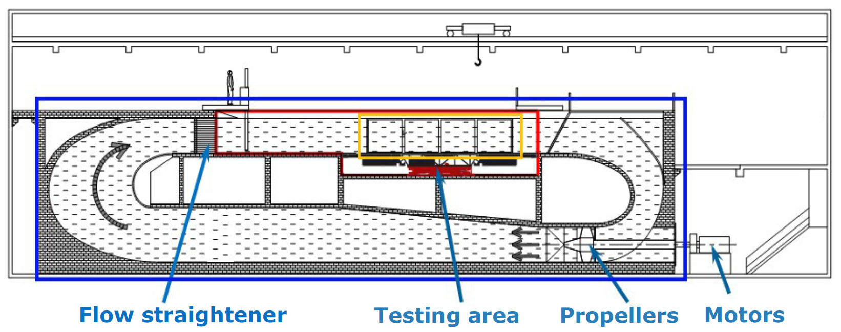
Experimental investigations are carried out in the wave and current flume tank of Ifremer at Boulogne-sur-mer, France, shown in Figure 1 [30]. The water is recirculated by two 250 kW motors and two propellers of 1 m in diameter, enabling 700 m³ of fresh water to be set in motion. The resulting current speeds range from 0.2 m/s to 2 m/s, in the testing area. This area is 18 m long by 4 m wide and $$h = 2 $$ m deep. In the present study, the streamwise flow velocity is fixed to $$U_{\infty} = 0 . 8 $$ m/s. The turbulence intensity is relatively low at 1.5 %. This low level of turbulence is reached through the use of a flow straightener at the inlet of the testing area.

Figure 1. Schematic of the wave and current flume tank of Ifremer (blue rectangle). The testing area (red rectangle) is 18 m long by 4 m wide and 2 m deep. The current velocities (grey arrows) range from 0.2 m/s to 2 m/s, with a turbulence intensity of 1.5 %. Four large windows (yellow rectangle) enable the flow velocity to be observed and quantified.

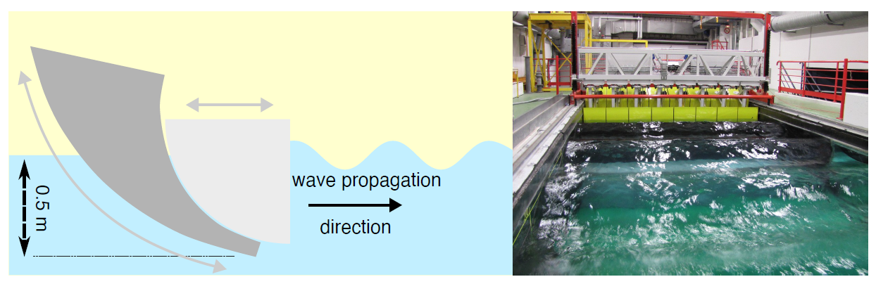
To generate water surface waves, a wave generator (Figure 2) is used for flow velocities up to 1.0 m/s. This generator consists of eight independent displacement paddles, each 0.5 m wide and 0.5 m deep, designed by Edinburgh Designs [31]. Each paddle uses a displacement technique that allows perfect flat front piston action while generating no back wave, as illustrated by the grey arrows showing the motions of the two parts, on the schematic of Figure 2. The wavemaker can generate both regular and irregular waves with a frequency range spanning from 0.25 Hz to 2 Hz, and a variable amplitude [32].

Figure 2. Schematic of the piston wave generator from Edinburgh Designs [31] (left-hand side). The grey arrows illustrate the displacements of the two parts of this paddle. The wavemaker of the Ifremer wave and current flume tank (right-hand side) is constituted of eight paddles like this one.

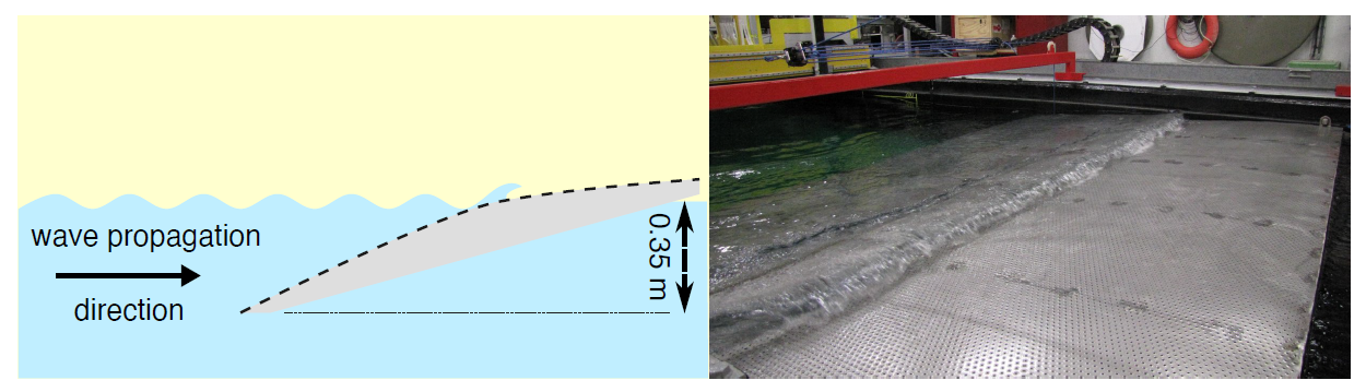
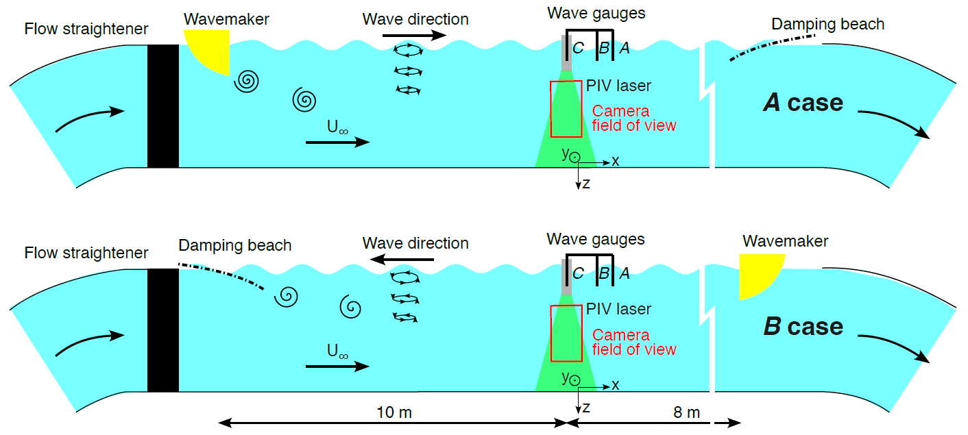
At the opposite side of the tank, a damping beach is positioned to break the waves (Figure 3). This damping beach is a parabolic porous plate, specifically designed for this flume tank and based on previous works [33]. The wavemaker and damping beach span the entire tank width. They can be easily reversed and positioned either upstream or downstream of the testing area. This allows for the generation of waves propagating with or against the current of the flume tank, with a maximum velocity of 1.0 m/s for both wave directions. The angle between wave and current is consequently 0° with waves following the current, or 180° with waves opposing the current. For the present study, this respectively corresponds to Case $$A$$ or Case $$B$$ of Figure 4. The $$\left( x , y , z \right)$$ cartesian coordinate system is used and it corresponds to the streamwise, transverse and vertical directions respectively.

Figure 3. At the opposite side of the wavemaker is the parabolic and porous damping beach, used for breaking the waves.

Figure 4. Experimental setup for the A case (top) where the waves propagate with current and for the B case (bottom) where the waves propagate against the current U_∞ (black arrows). The PIV measurement plane (red rectangle) is roughly located in the center of the test section of the tank and vertically aligned with the wave gauge C.

It’s important to note that this experimental setup is quite specific. The presence of the wavemaker or damping beach about 10 m upstream from the measurement location generates a turbulent wake flow which affects the measurements. The submergence depths of the wavemaker and damping beach are $$D_{g} = 0 . 5$$ m and $$D_{a} = 0 . 35$$ m respectively (see Figure 2 and Figure 3). As shown schematically in Figure 4, for each case ($$A$$ or $$B$$), these two obstacles generate some large-scale flow structures that slowly fall down into the water column of the tank, carried away by the current. This setup allows for the study of the effects of the wave direction on the development of these large-scale flow structures in the water column. The flow Reynolds number is $$R e = U_{\infty} D / \nu = 3 . 4 \times 10^{5}$$, with $$D = 0 . 425$$ m the mean submergence depth of both upstream obstacles (wavemaker or damping beach) and $$\nu$$ the kinematic viscosity of water. To reproduce sea-wave conditions, a monochromatic wave frequency of 0.45 Hz and an amplitude of approximately 0.05 m is imposed by the wavemaker to the flow velocity of $$U_{\infty} = 0 . 8$$ m/s, with:

1.: Case $$A$$ (denoted $$A_{w a v e}$$): Wave following the Current
2.: Case $$B$$ (denoted $$B_{w a v e}$$): Wave opposing the Current

These experimental parameters align with previous studies [26] and replicate sea conditions found in the English Channel, particularly at sites of significant interest for marine renewable energy. These wave characteristics roughly correspond to a 10 s peak period with significant wave height of 2 m, at a scale of 1:20 and a Froude number of 0.17 [34]. Associated with a tidal flow velocity of 3.5 m/s, these marine conditions correspond to a relatively severe in-situ wave and current combination. In both cases, the waves remain largely two-dimensional, with very limited transverse ($$y$$) side effect. To state about the wave effects on the water column flow, two additional configurations are considered with the wavemaker idle and the same flow velocity of $$U_{\infty} = 0 . 8$$ m/s. These two additional cases will be denoted $$A_{n o\, w a v e}$$ and $$B_{n o \,w a v e}$$ respectively in the following (see Table 1).

Table 1. Detail of the four flow configurations considered in the present study. See Figure 4 for the detail of the device located at the upstream (US) position from the testing area. When wavemaker is upstream, waves are generated following the current. When wavemaker is downstream, waves are generated opposing the current. In the following, each flow configuration will be referred to the label and symbol mentioned in this table.

Cases	A Case: Wavemaker US		B Case: Damping Beach US
Wavemaker	Idle	Active	Idle	Active
Wave direction	no wave	Following	no wave	Opposing
Label	$$A_{n o\, w a v e}$$	$$A_{w a v e}$$	$$B_{n o\, w a v e}$$	$$B_{w a v e}$$
Symbol	$$○$$	$$\Huge\Huge\bullet$$	$$\triangledown$$	$$\blacktriangledown$$

2.1. Wave Surface Measurements The wave properties (amplitude, wavelength, frequency) are measured using 3 wave probes: a Kenek servo-type wave probe (model SHT3-30E) and 2 resistive wave probes. The dynamic Kenek wave probe is marked with the letter $$A$$ in Figure 4 and the two other probes are installed on positions $$B$$ and $$C$$. The distances between these points are $$\left[ A B \right] = 52$$ cm and $$\left[ B C \right] = 70$$ cm. The wave gauge $$C$$ is vertically aligned with the center of the Particle Image Velocimetry (PIV) measurement plane (red rectangle in Figure 4). A regular calibration is required during the measurement campaign to keep the accuracy of these wave gauges lower or equal to 3 mm. Wave measurement acquisition is synchronised with the PIV system via a shared trigger. 2.2. Particle Image Velocimetry Measurements Particle Image Velocimetry measurements are carried out in a vertical plane $$\left( x , z \right)$$, as illustrated with the red rectangle in Figure 4. This plane is roughly located at the streamwise center of the tank. In this area, the turbulent wake developing behind either the wavemaker or the damping beach is fully developed in the water column. It is also worth noting that the tank is sufficiently deep that the developing bottom boundary layer does not interact with the obstacle wake flows. The PIV sampling frequency is $$f_{P I V} = 15$$ Hz and $$N_{t} = 2700$$ instantaneous velocities $$\left( u , w \right)$$ are acquired in the vertical $$\left( x , z \right) -$$plane of $$\left( N_{x} , N_{z} \right) = \left( 41 , 79 \right)$$ points, with a spatial discretisation of 11.6 mm in each direction. The sum of uncertainties concerning the PIV measurement is evaluated to 6.7 % [35], i.e., 0.054 m/s for the flow velocity of $$U_{\infty} = 0 . 8$$ m/s of this study. The $$x$$-axis origin is taken at the right position of the PIV measurement plane. The $$z$$-axis origin is fixed at the bottom of the tank, and the PIV measurement plane is centred in the vertical water depth, as depicted in Figure 4. Such a choice is due to help future investigations of the interactions between the wave turbulent flow and a tidal turbine model or an offshore wind turbine support structure. The classical Reynolds decomposition is first applied to the instantaneous PIV velocity field as follows:

```latex\begin{cases}u(x,z,t)=\overline{U}(x,z)+u^{\prime}(x,z,t)\\w(x,z,t)=\overline{W}(x,z)+w^{\prime}(x,z,t)&\end{cases}```

(1)

where an overbar indicates the time average operator and $$\left( u^{\prime} , w^{\prime} \right)$$ corresponds to the instantaneous fluctuating velocity field. In the present work, we do not attempt to separate the turbulent and the wave-induced components. The main interest of this study lies in the characterisation of the velocity fluctuations in the water column, in order to understand the wave effects on large-scale turbulent flow structures better. Before making comparisons between flows with and without waves, the main properties of both wake flows $$A_{n o \,w a v e}$$ and $$B_{n o\, w a v e}$$ are investigated in the following section.

3. Global Flow Analysis of the Current without Wave

The analysis of the $$A_{n o \,w a v e}$$ and $$B_{n o\, w a v e}$$ flow configurations is conducted in this section. For each case, the incoming flow interacts with the wavemaker ($$A$$ case) or the damping beach ($$B$$ case) and a turbulent wake flow is then generated behind each obstacle. As discussed in the introduction, the flow conditions in the water column significantly impact the performan-ce and lifespan predictability of marine structures. These two parameters depend on several flow characteristics: the mean velocity shear [36], the turbulence intensity [37,38], the large-scale flow structures and its associated frequency passage [11,39], the integral length scale [12,40], and the flow Gaussianity [12,41]. Therefore, accurately characterising these incoming flow characteristics is crucial for evaluating and quantifying their effects. Subsequently, these different flow characteristics are successively determined, allowing for a comparison of the wave effect in the next section. 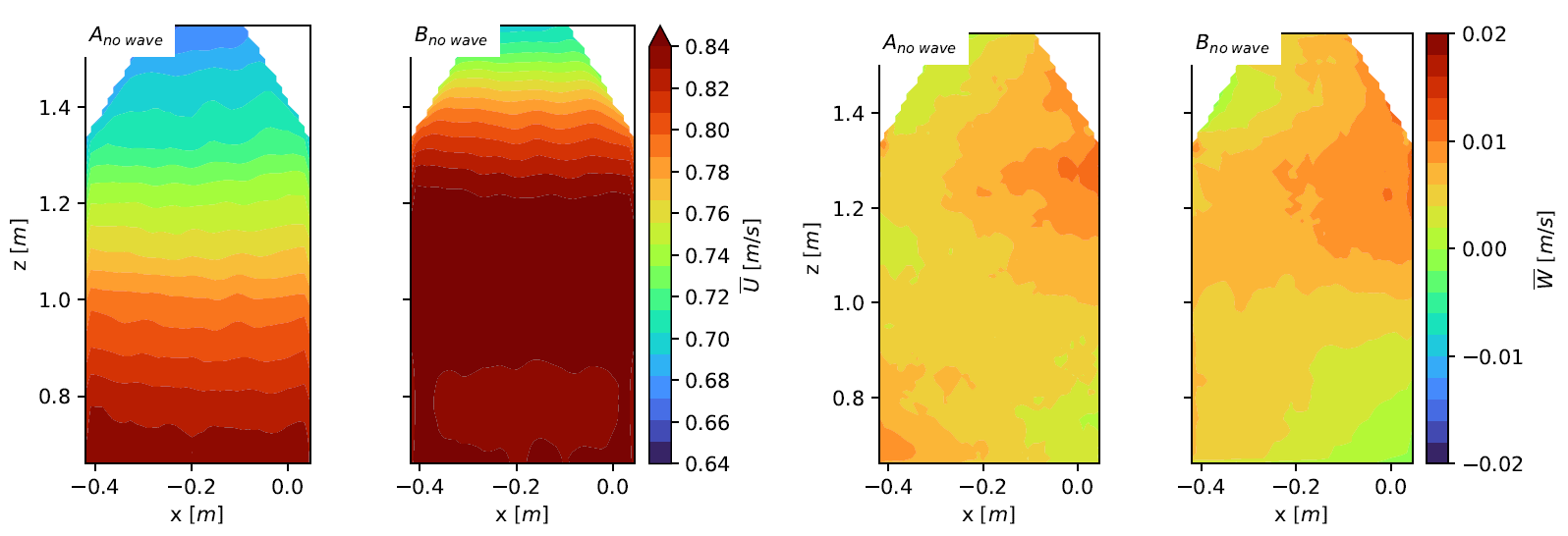Figure 5 displays the colormaps of the mean velocity components for both cases. The mean streamwise velocity component exhibits a clear shear velocity profile along the vertical extent. Note that in the present flow configurations, the velocity gradient is negative in the water column that differs from previous analyses [26]. The velocity shear is more pronounced for the $$A$$ case as the submergence depth of the idle wavemaker is higher than the one of the damping beach. Furthermore, the shear velocity profile is mainly present for $$z > 1 . 2$$ m for the $$B_{n o \,w a v e}$$ case while it covers the whole vertical extent of the PIV plane until $$z = 0 . 6$$ m. The amplitude of $$\overline{W}$$ is of the same order of magnitude in both cases. 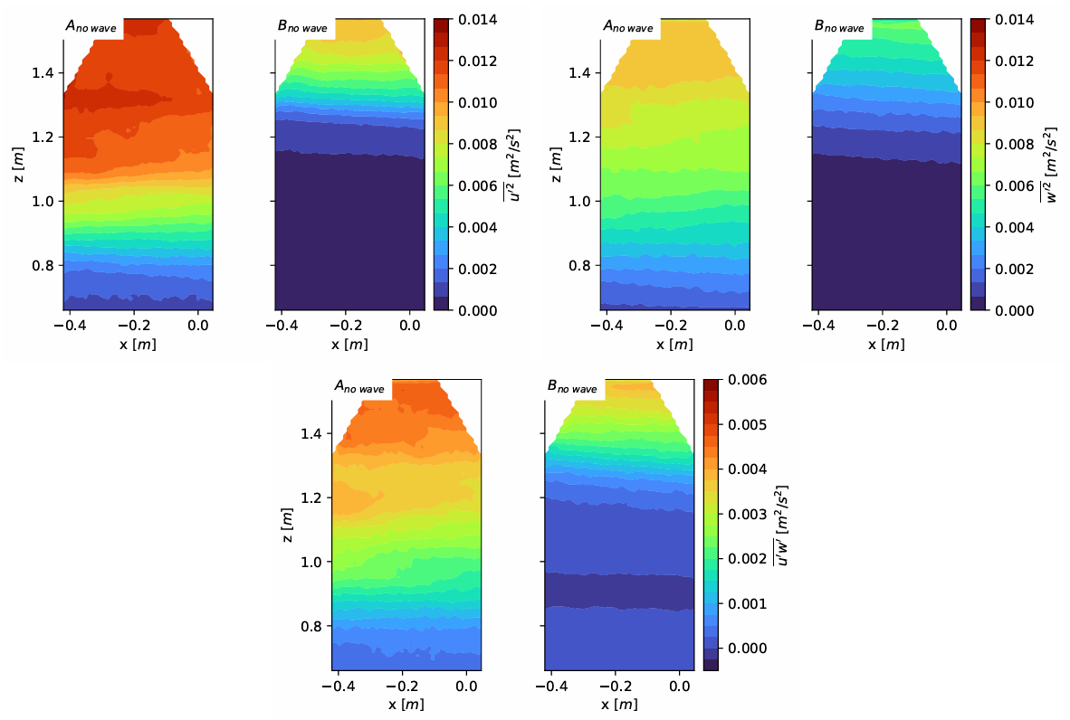Figure 6 represents the colormap of the 3 Reynolds shear stresses $$\overline{u^{\prime2}},\overline{w^{\prime2}}$$ and $$\overline{u^{\prime}w^{\prime}}$$. As expected, the highest amplitudes of the stresses are observed for the $$A$$ case, where the mean velocity exhibits a more pronounced shear than in the $$B$$ case. In this latter case, the main kinetic energy is located at the top part of the measurement plane, corresponding to large-scale flow structures.

Figure 5. Isosurface of the mean axial velocity $$\overline{U}$$ (left-hand side) and the mean vertical velocity $$\overline{W}$$ (right-hand side) for both $$A$$ and $$B$$ flow cases with no wave.

Figure 6. Isosurface of the Reynolds tensor components $$\overline{u^{\prime2}}$$ (top, left-hand side), $$\overline{w^{\prime2}}$$ (top, right-hand side) and $$\overline{u^{\prime}w^{\prime}}$$ (bottom) for both $$A$$ and $$B$$ flow cases with no wave.

To investigate the turbulent wake flow organisation, a Fourier analysis is performed to examine the large-scale periodic flow structures. First, the instantaneous fluctuating streamwise velocity component $$u^{\prime} \left( t , z \right)$$ is extracted at each vertical position along the centre line located at $$x_{0} = - 0 . 2$$ m of the PIV measurement plane. Next, the spectral analysis of the recorded $$u^{\prime} \left( t , z \right)$$ signal is processed using the PSD function based on Welch’s method [42] in Python [43] with a Hann window function. 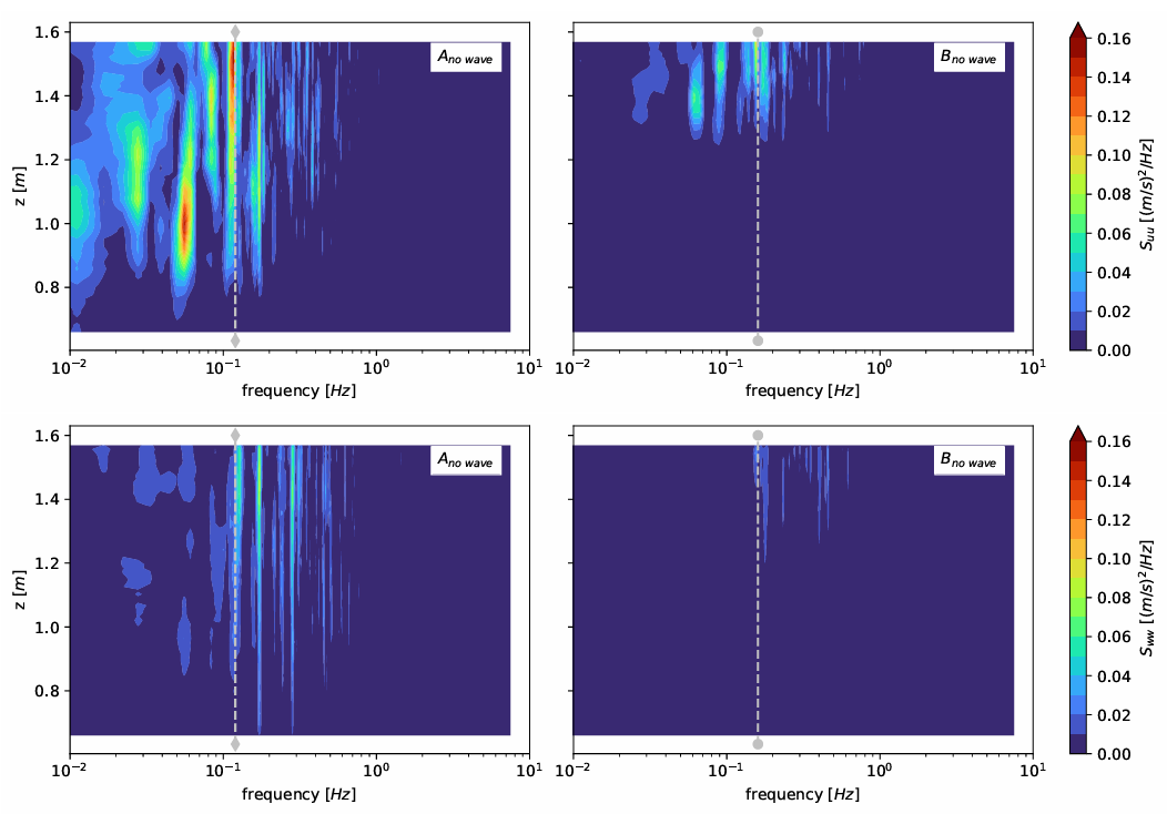Figure 7 presents the PSD maps for both flow cases. The presence of the wavemaker induces a wake flow exhibiting a spectral frequency peak around $$f_{g} = 0 . 12$$ Hz in the water column, highlighted by the diamond markers. This corresponds to the Strouhal number of $$S_{t} = f_{g} D_{g} / U_{\infty} = 0 . 07$$. Similarly, the wake of the damping beach, which has a submergence depth of $$D_{a} < D_{g}$$, shows a frequency peak around $$f_{a} = 0 . 16$$ Hz (circle markers), also corresponding to a Strouhal number of $$S_{t} = f_{a} D_{a} / U_{\infty} = 0 . 07$$. This Strouhal value is in agreement with peak values associated with the shedding frequency observed in previous dune flow simulations [44] and in the wake of a wall-mounted cylinder [8]. Note that for the $$B_{n o\, w a v e}$$ flow case, the large-scale periodic flow structures are only detectable in the upper part of the measurement plane $$z > 1 . 3$$ m, as discussed previously following the mean flow analysis.

Figure 7. PSD maps of the fluctuating streamwise $$u^{\prime}$$ (top) and vertical $$w^{\prime}$$ (bottom) velocity components along the vertical line located at $$x_{0} = - 0 . 2$$ m for both flow cases with no wave. The grey dashed lines correspond to a Strouhal number of 0.07 linked to the shedding frequencies downstream from the idle wavemaker (diamond markers, at $$f = 0 . 12$$ Hz, for the $$A_{n o\, w a v e}$$ case) or damping beach (circle markers, at $$f = 0 . 16$$ Hz, for the $$B_{n o \,w a v e}$$ case).

To determine the statistical size of the energetic flow structures in each flow case, the integral length scale $$L_{u}$$ associated with the streamwise velocity component is computed. At each point of the PIV measurement plane, the procedure detailed previously [45] is followed. First, the integral time scale $$T_{u} \left( z \right)$$ is estimated by integrating the autocorrelation of the fluctuating streamwise velocity signal $$u^{\prime} \left( z \right)$$ to a specified threshold of 0.1. Then, the integral length scale is determined using the Taylor hypothesis under frozen turbulence: $$L_{u} \left( z \right) = \overline{U} \left( z \right) T_{u} \left( z \right)$$, where $$\overline{U} \left( z \right)$$ is the local mean streamwise velocity component for each flow configuration. 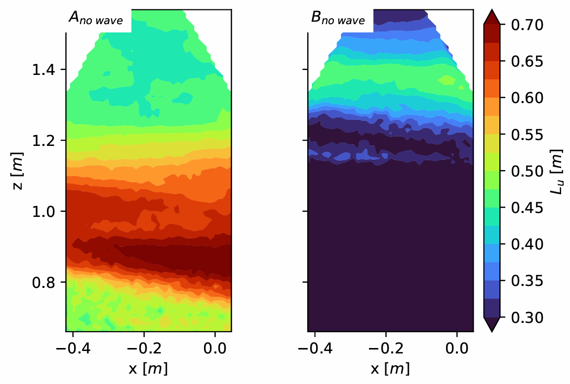Figure 8 displays the isosurface of $$L_{u} \left( z \right)$$ for both cases with no wave. For $$A_{n o \,w a v e}$$ case, the large-scale flow structures developing behind the wavemaker are clearly noticeable. These structures are observed in the water column for $$z$$ between 0.8 m and 1.1 m, with a size of approximately $$L_{u} = 0 . 7$$ m to $$ 0 . 8$$ m. Conversely, the integral length scales measured for the $$B_{n o\, w a v e}$$ case are smaller. There is a noticeable increase around $$z = 1 . 4$$ m, with a corresponding size of about $$L_{u} = 0 . 5$$ m. These length scales are related to the large-scale periodic flow structures detected in this area, as confirmed by the previous spectral analysis. On the bottom part ($$z < 1 . 2$$ m), the temporal correlation does not reveal any noticeable integral length scale ($$L_{u} < 0 . 3$$ m) as the flow is uniform and of very low energetic content.

Figure 8. Isosurface of the integral length scale for both $$A$$ and $$B$$ flow configurations with no wave.

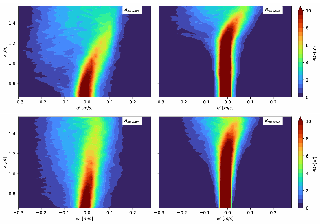
Based on previous analyses, the main flow parameters remain relatively constant across the streamwise extent of the measurement plane. To enhance the comparative analysis between wave and no-wave cases (see Section 5), we now focus on measurements along the vertical centre line of the PIV plane, at $$x_{0} = - 0 . 2$$ m. The flow Gaussianity is investigated in the water column along this line by analysing the normalised Probability Density Function (PDF) histograms of both fluctuating $$u^{\prime}$$ and $$w^{\prime}$$ velocity components (Figure 9).

Figure 9. Normalised PDF histograms of the fluctuating $$u^{\prime}$$ velocity component (top) and $$w^{\prime}$$ velocity component (bottom) along the vertical line located at $$x_{0} = - 0 . 2$$ m for both flow cases with no wave.

At the bottom part of the measurement plane, the flow is predominantly uniform and unaffected by the passage of large-scale flow structures. Consequently, the fluctuating velocities exhibit a Gaussian-like distribution. As we ascend the water column, the PDF distributions begin to deviate from Gaussian-like distribution due to the presence of large-scale flow structures. The PDF distributions become asymmetric from $$z > 0 . 8$$ m in the $$A_{n o\, w a v e}$$ case and from $$z > 1 . 2$$ m in the $$B_{n o \,w a v e}$$ case. This observation aligns with previous results and the vertical extent of the large-scale flow structures in the water column, observed in the wake of wall mounted obstacles [12]. The largest fluctuations originate from the dominant large-scale energetic flow structures. In summary, the wake of the wavemaker ($$A_{n o\, w a v e}$$ case) induces a velocity shear flow that spans the entire vertical extent of the measurement plane for $$z \in \left[ 0 . 6 , 1 . 6 \right]$$. However, since the submergence depth of the damping beach is shallower than that of the wavemaker, the velocity shear observed for the $$B_{n o\, w a v e}$$ case is only present for $$z > 1 . 2$$ m, at the same streamwise location. In both flow cases, large-scale flow structures are identified and associated with a low-frequency signature. These structures are more energetic and larger for the $$A$$ case compared to the $$B$$ case. Consequently, for the $$A_{n o\, w a v e}$$ case, the local turbulence level in the water column is greater than that observed for the $$B_{n o\, w a v e}$$ case.

4. Analysis of the Surface Water Wave

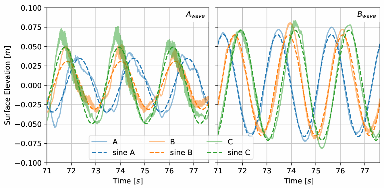
For each wave and current case ($$A_{w a v e}$$ and $$B_{w a v e}$$), the wavemaker generates a regular sinusoidal wave with a frequency of $$f_{w} = 0 . 45$$ Hz. Figure 10 shows an extract of the time history of the wave elevation recorded by the three wave gauges for both wave cases. From this time extract, it is clear that the $$B_{w a v e}$$ case shows a higher amplitude of surface elevation compared to the $$A_{w a v e}$$ case. Additionally, the noise level is higher for the signals recorder for the $$A_{w a v e}$$ case compared to the $$B_{w a v e}$$ case. As mentioned in Section 2, the wavemaker is more intrusive in the water column than the damping beach, with $$D_{g} > D_{a}$$. Consequently, close to the free surface, the flow is more impacted by the presence of the wavemaker, and these higher flow perturbations more impact the wave generation. Therefore, due to the surface distortion effects linked to the current perturbations of the upstream wavemaker ($$A_{w a v e}$$ case) or damping beach ($$B_{w a v e}$$ case), the wave amplitudes vary over time. The wave reflection level is of the order of 10 % with no flow in the tank [32]. Assuming this reflection rate remains similar when the flow velocity is $$U_{\infty} = 0 . 8$$ m/s, the wave amplitudes are also influenced by this effect.

Figure 10. Time evolution of the wave amplitude recorded by the 3 wave gauges (solid line) superimposed onto sinusoidal signal at $$f_{w} = 0 . 45$$ Hz (dashed line), for both wave cases.

The results presented in this paper are part of a larger dataset. Tests were repeated multiple times within this dataset, always using the exact same flow configurations and for a constant 3-min acquisition time. The only parameter that was changed was the position of the wave gauges in the tank, while the inter-distances between the probes remained identical. Finally, all these acquisitions (25 runs for $$A_{w a v e}$$ case and 15 runs for $$B_{w a v e}$$ case) enable the average wave characteristics to be processed with high confidence using the measurements from the three wave gauges. The data processing used to determine the wave amplitude and phase involves finding the best fit for each wave gauge measurement. This is achieved using a least squares method, assuming the signals are pure sine function of the form:

```latex\eta \left( t \right) = A_{w} \sin \left( \omega t + \varphi \right)```

(2)

where $$\omega = 2 \pi f_{w}$$ and supposing $$\overline{\eta(t)}=0$$. These sine functions are plotted on Figure 10 with dashed lines for comparison with the recorded wave gauges (solid lines). The wave amplitude is determined by the different values obtained for $$A_{w}$$ from the sine functions calculated for the three wave gauges across all tests. The wavelength $$\lambda$$ is calculated using the phase $$\varphi$$ of the three wave gauges and their relative inter-distances, following the formula:

```latex\lambda = 2 \pi \frac{x_{i} - x_{j}}{\varphi_{i} - \varphi_{j}}```

(3)

with indices $$i$$ and $$j$$ corresponding to the three wave gauges, and $$x$$ their respective positions in the tank. Wave amplitudes and wavelengths results are summarised in Table 2 for both wave-current configurations. Additionally, Table 2 provides the corresponding standard deviations for the averaged values of $$A_{w}$$ and $$\lambda$$ obtained from the overall acquisitions.

Table 2. Wave characteristics generated in the flume tank.

Case	$$\bm{f}_{\bm{w}}$$ [Hz]	$$\bm{A}_{\bm{w}}$$ [mm]	$$\bm{\lambda}$$ [m]	$$\bm{h} / \bm{\lambda}$$
$$A_{w a v e}$$	$$0 . 45$$	$$42 \pm 9$$	$$9 . 9 \pm 8 . 5$$	$$0 . 2$$
$$B_{w a v e}$$	$$0 . 45$$	$$69 \pm 2$$	$$3 . 9 \pm 1 . 4$$	$$0 . 5$$

As observed on Figure 10, the wave amplitude is higher for the $$B_{w a v e}$$ case because the current faces the wave propagation. On the contrary, for the $$A_{w a v e}$$ case, the wave and current propagate in the same direction, resulting in a smaller wave amplitude. The wavelength evolution is the opposite: the highest wavelengths are measured for the $$A_{w a v e}$$ case. This is because the wavelength increases when the current and waves are in the same direction and decreases when they move in opposite ways, as classically observed [46]. The standard deviations given in Table 2 show relatively large values, especially for the wavelength $$\lambda$$ of the $$A_{w a v e}$$ case. As mentioned before, this is related to wave generation with the flow perturbation originating from the wavemaker located upstream. Additionally, the inter-distances of the wave gauges, ranging from 0.5 m to 1.2 m, are relatively low compared to the wavelength of approximately 10 m. Since these inter-distances are less than 10 % of the wavelength, the phase differences $$\left( \varphi_{i} - \varphi_{j} \right)$$ are also very small. Consequently, according to Equation (3), this can explain large standard deviation of $$\lambda$$. Finally, these 2 wave and current cases have the same wave frequency and show an amplitude of roughly the same order of magnitude. The only difference is the wave direction, which changes compared to the current direction (following or opposing). This change in direction results in a different wave propagation velocity, which in turn affects the wavelength. Both wave cases fall within the same wave classification of intermediate water depth [47], with $$0 . 05 < h / \lambda < 0 . 5$$ and $$h = 2$$ m the water depth. 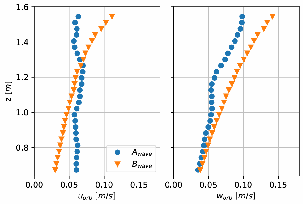Figure 11 shows the amplitudes of wave orbital velocities within the water column. These amplitudes are derived from PIV measurements using a similar method to that employed for wave gauges. Specifically, a best-fit sine function, determined through a least squares approach, is applied to the 2 components of the PIV velocities. The amplitudes of these sine functions, noted $$u_{o r b}$$ and $$w_{o r b}$$, are then extracted for each vertical position. Profiles obtained for the $$B_{w a v e}$$ case appear exponential, with significant variations versus the depth. Conversely, $$A_{w a v e}$$ profiles are more constant with the depth, particularly for the axial velocity component $$u_{o r b}$$. These observations corroborate the wave classification established from characteristics showed in Table 2, placing the $$B_{w a v e}$$ case at the limit between intermediate and deep water waves [47].

Figure 11. Amplitudes of wave orbital velocities measured from PIV acquisitions, from the best-fit of each velocity component using a least squares method, for both wave and current cases.

5. Effect of Waves on Wake Flow Dynamics

In the following section, the PIV velocity measurements are analysed along the vertical line at $$x_{0} = - 0 . 2$$ m, which is the center of the PIV measurement plane. This profile is chosen to quantify the mean velocity and the main flow fluctuation characteristics. The section concludes with an analysis of the kinetic energy budget and results from a quadrant method. 5.1. Mean Velocity Analysis in the Water Column Figure 12 shows the vertical profiles of the mean velocity components $$\overline{U}$$ and $$\overline{W}$$ for each flow case. These profiles are normalised with a reference velocity $$U_{r e f}$$, which is the spatial average of $$\overline{U}$$ over the vertical extent. For both $$A$$ cases ($$A_{n o\, w a v e}$$, $$A_{w a v e}$$), $$U_{r e f}$$ is identical and equal to 0.76 m/s. For both $$B$$ cases ($$B_{n o\, w a v e}$$, $$B_{w a v e}$$), $$U_{r e f}$$ is quasi-similar, with a very small difference of 1.5% between them, and $$U_{r e f} = 0 . 81$$ m/s. For $$A$$ cases, the velocity gradient increases in presence of waves, while it seems to remain similar for the $$B$$ cases. By extrapolating the mean velocity towards the water surface, the mean streamwise velocity decreases when waves propagate with the current ($$A_{w a v e}$$ case). On the contrary, it is expected that $$\overline{U}$$ increases when waves propagate against the current ($$B_{w a v e}$$ case), confirming previous studies on the effects of wave-current interactions on the logarithmic boundary layer velocity profile [48,49] and on the vertical shear velocity profile [22]. However, the presented results, which are limited to partial depth measurements, do not provide evidence for this. The mean $$\overline{W}$$ profiles follow a similar tendency with or without waves. However, vertical oscillations are clearly visible in the presence of waves, regardless of the wave direction. These oscillations can be attributed to the vertical component of the orbital velocity of the waves propagating through the water column. They are perceived here because the mean vertical velocity component of the current is of the same order of magnitude as the mean amplitude of the vertical wave orbital velocity component. Globally, the wave and current mean velocity profiles closely resemble those of turbulent flow without wave components, though slight differences can be observed.

Figure 12. Vertical profiles of the mean velocity component ($$\overline{U}$$ at the left-hand side and $$\overline{W}$$ at the right-hand side) with waves (filled markers) and with no wave (empty markers) for both $$A$$ and $$B$$ flow cases, extracted along the line at $$x_{0} = - 0 . 2$$ m.

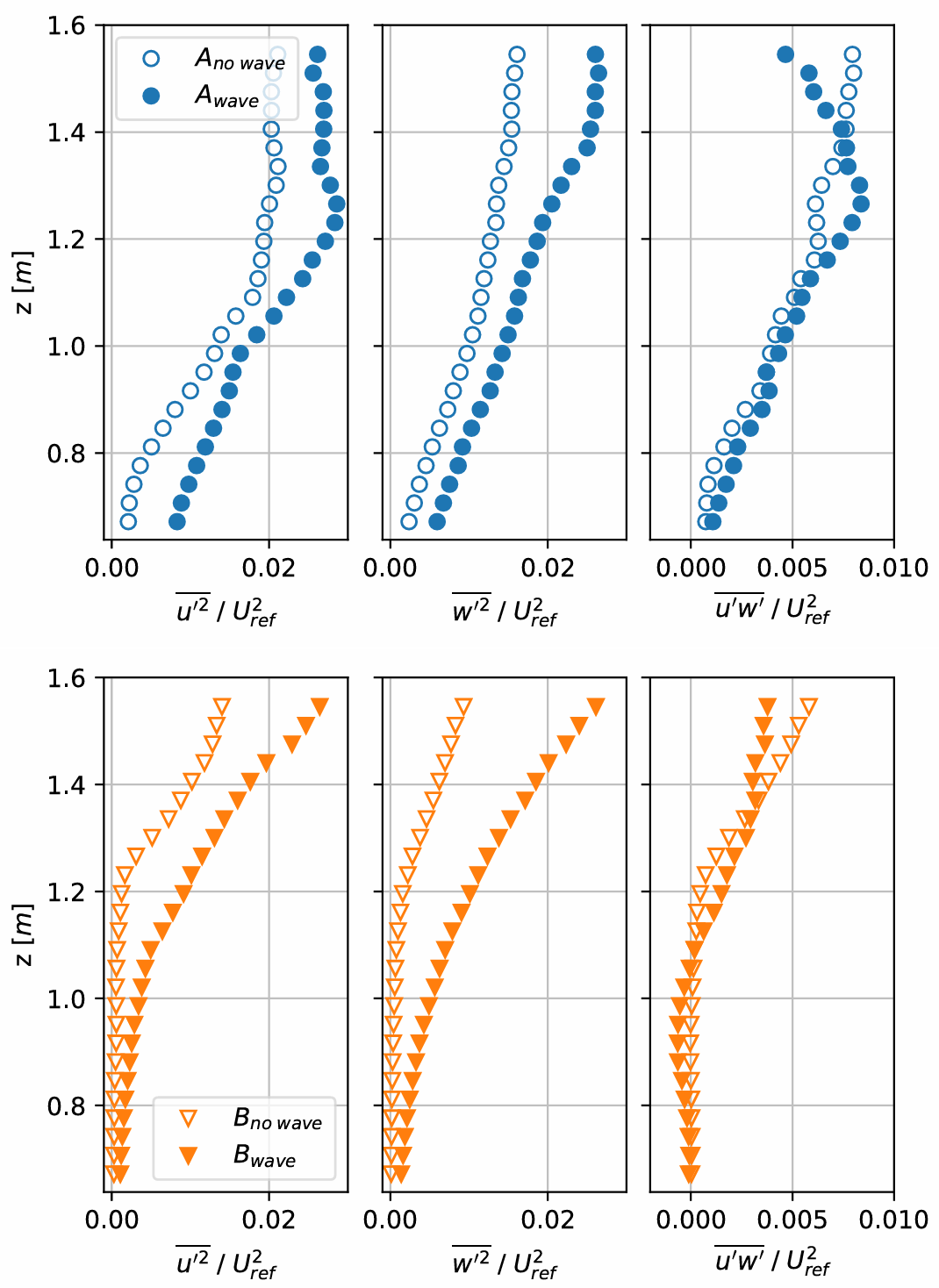
5.2. Turbulence Statistics in the Water Column Figure 13 presents vertical profiles of the Reynolds tensor components: $$\overline{u^{\prime2}}/U_{ref}^2,\overline{w^{\prime2}}/U_{ref}^2$$ and $$\overline{u^{\prime}w^{\prime}}/U_{ref}^2$$. Regardless of the wave direction ($$A$$ or $$B$$ case), the wave and current components consistently exhibit higher amplitudes compared to those calculated in pure current cases, as previously observed [26]. This is because waves inject kinetic energy into the water column, thereby increasing the turbulent kinetic energy in the turbulent flow. The vertical component, $$\overline{w^{\prime2}}/U_{ref}^2$$, appears to be more influenced by waves than the horizontal one, $$\overline{u^{\prime2}}/U_{ref}^2$$, particularly when waves propagate against the current ($$B_{w a v e}$$ case). Consequently, waves exert a more pronounced influence on the vertical mixing associated with the velocity fluctuations $$w^{\prime}$$. The associated kinetic energy gradually increases towards the free surface, as waves contribute more energy to the current near the surface. This results in larger turbulent intensities near the free surface, as the wave effect on turbulent flows increases. The wave propagation within the water column is also evident in the shear Reynolds stress component, $$\overline{u^{\prime}w^{\prime}}/U_{ref}^2$$, at the upper part of the water column, where the shear component is reduced near the water surface. The momentum transport in the vertical direction is then locally modified by the wave forcing, as demonstrated by the analysis of the turbulent kinetic energy production in Section 5.6. This finding aligns with previous observations [50], when examining the interaction between waves and the flow of the bottom boundary layer.

Figure 13. Vertical profiles of the normalised Reynolds stress components $$\overline{u^{\prime2}}/U_{ref}^2$$ (left-hand side), $$\overline{w^{\prime2}}/U_{ref}^2$$ (center) and the shear component $$\overline{u^{\prime}w^{\prime}}/U_{ref}^2$$ (right-hand side) for both $$A$$ and $$B$$ flow cases with waves (filled markers) and with no wave (empty markers), extracted along the line at $$x_{0} = - 0 . 2$$ m.

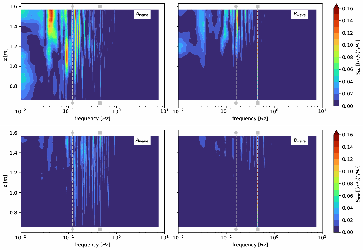
5.3. Spectral Analysis in the Water Column As previously done for current alone cases (see Section 3), the PSDs associated with $$u^{\prime} \left( t , z \right)$$ and $$w^{\prime} \left( t , z \right)$$ are determined and represented as a function of frequency on horizontal axis and vertical position on vertical axis, in Figure 14. The same procedure detailed in Section 3 is followed for each case. These figures can be directly compared to Figure 7 for current alone cases, using a similar colormap. On these graphs, the wave signature frequency ($$f_{w} = 0 . 45$$ Hz) is clearly visible in the water column, with a higher amplitude in the upper part. The square markers highlight this frequency. For $$A$$ cases, the low-frequency signature of the large-scale periodic structures differs slightly between current alone and when waves propagate with the current. In the $$A_{n o \,w a v e}$$ case (Figure 7), the main frequency peak is observed at $$f = 0 . 12$$ Hz for $$z > 1 . 2$$ m, corresponding to a Strouhal number of 0.07 and highlighted by diamond markers. For the $$A_{w a v e}$$ case (Figure 14), the PSD of $$u^{\prime}$$ similarly exhibits a main frequency peak at $$f \simeq 0 . 14$$ Hz for $$z > 1 . 2$$ m. Therefore, when waves propagate with the current, the low-frequency flow structures are slightly impacted by an increase in the associated frequency passage due to the non-linear wave-current interactions. In addition, several low-frequency peaks appear at $$f \simeq 0 . 04$$ Hz around $$z \simeq 1 . 5$$ m and $$f \simeq 0 . 08$$ Hz at $$z \simeq 1 . 1$$ m. These peaks differ from those observed in the current-only case. When analysing the PSD of the $$w^{\prime}$$ component, the $$A_{w a v e}$$ case exhibits multiple peaks between $$f \simeq 0 . 14$$ Hz and $$f_{w} = 0 . 45$$ Hz. These peaks are probably related to a combination of large-scale flow structures shedding frequency and wave frequency. When waves propagate against the current ($$B_{w a v e}$$ case), the PSD of $$u^{\prime}$$ shows a main frequency peak at the wave frequency $$f_{w}$$ with decreasing amplitude as $$z$$ decreases. Additionally, the low-frequency peak associated with the large-scale flow structures developing behind the damping beach has a higher amplitude than the one observed in current-only case ($$B_{n o \,w a v e}$$, see Figure 7). This confirms that wave energy is injected into the water column. Consequently, the large-scale periodic flow structures have higher energy and are detected over a deeper distance in the water column.

Figure 14. PSD maps of the $$u^{\prime}$$ (top) and $$w^{\prime}$$ (bottom) velocity components along the vertical line at $$x_{0} = - 0 . 2$$ m, for both $$A$$ and $$B$$ flow cases with waves. The grey dashed lines with diamonds and circles correspond to a Strouhal number of 0.07 previously observed on Figure 7 (no wave cases). The grey dashed lines with square markers stand for the wave frequency $$f_{w} = 0 . 45$$ Hz.

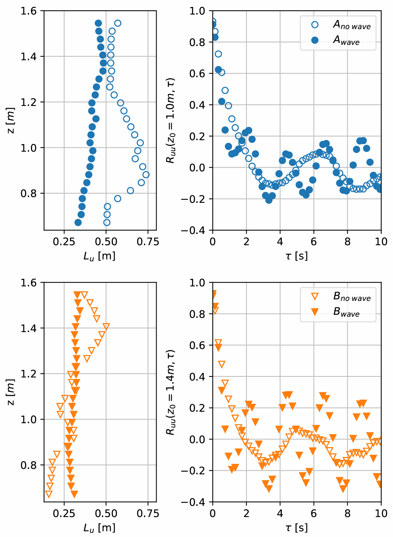
5.4. Integral Length Scale Analysis in the Water Column Figure 15 illustrates the vertical profile of the integral length scale calculated for each case. The determina-tion follows the procedure outlined in Section 3. It is very interesting to observe that the presence of waves, either with or against the current, significantly influences the integral length scale values. For each case, the associated values are approximately 40% smaller than those computed for the current-only cases. These high values are related to the large-scale flow structures at $$z \simeq 1 . 0$$ m ($$A_{n o\, w a v e}$$ case) and $$z \simeq 1 . 4$$ m ($$B_{n o \,w a v e}$$ case) respectively. This result directly stems from the instantaneous wave effect in the water column, which generates a periodic oscillatory perturbation. Figure 15 (right-hand side) presents the temporal correlation of the streamwise velocity component $$R_{u u} \left( x_{0} , z_{0} , \tau \right)$$ used to compute the integral time scale:

```latexR_{uu}(x_0,z_0,\tau)=\frac{\overline{u^{\prime}(x_0,z_0,t)u^{\prime}(x_0,z_0,t+\tau)}}{\overline{u^{\prime}u^{\prime}}}```

(4)

with $$z_{0} = 1 . 0$$ m ($$A$$ case) and $$z_{0} = 1 . 4$$ m ($$B$$ case). These positions correspond to the area where large-scale flow structures occur. The wave period ($$1 / f_{w}$$) signature is then clearly visible in the temporal correlation signal related to wave cases. The wave action limits the temporal correlation of the velocity signal at each specific $$z$$ location, greatly reducing the temporal length scale and the integral streamwise scale. More specifically, these results differ from previous ones dealing with a negatively vertical sheared current [24], where it was observed that the integral length scales increase with waves, regardless of their direction. This is a consequence of the vertical mixing, which differs as a function of the incoming vertical shear current, while the vertical shear of the wave velocity field remains the same regardless of the incoming flow (Section 5.6).

Figure 15. Left-hand side: vertical profiles of the integral length scales, extracted along the line at $$x_{0} = - 0 . 2$$ m; Right-hand side: time correlation of the axial velocity component $$R_{u u}$$ from the point $$\left[ x_{0} ; z_{0} \right]$$; for both $$A$$ (top) and $$B$$ (bottom) flow cases with waves (filled markers) and with no wave (empty markers). $$z_{0} = 1 . 0$$ m for $$A$$ cases and $$z_{0} = 1 . 4$$ m for $$B$$ cases.

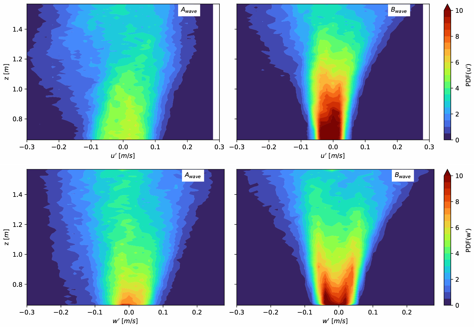
5.5. Flow Gaussianity Analysis in the Water Column To assess the Gaussianity of each flow configuration, the PDF histograms of both velocity fluctuating components $$u^{\prime}$$ and $$w^{\prime}$$ are determined in the water column (Figure 16) and compared to previous results for the current-only cases (Figure 9). The PDFs of the fluctuating velocity fields measured in the wave flow configurations ($$A_{w a v e}$$ and $$B_{w a v e}$$ cases) significantly differ from those determined in the pure current cases. In both cases, a quite similar pattern is observed in the PDF of $$u^{\prime}$$ component. The PDF distribution is asymmetric throughout the water column, with alternating positive and negative values along the $$z$$ direction, particularly when waves propagate with the current. The wave properties directly influence this modulation. The wave oscillations enhance and spread of the smaller-scale fluctuations. Similar observations can be made for the PDF of the $$w^{\prime}$$ component in the $$A_{w a v e}$$ case. Conversely, for the $$B_{w a v e}$$ case, the PDF of $$w^{\prime}$$ exhibits a bimodal distribution for $$z < 1$$ m and a negative fluctuation peak is predominantly present for $$z > 1$$ m. This bimodal representation has been previously observed in wave-against-tidal-current flow configuration [22].

Figure 16. Normalised PDF histograms of the fluctuating streamwise $$u^{\prime}$$ (top) and vertical $$w^{\prime}$$ (bottom) velocity components along the vertical line located at $$x_{0} = - 0 . 2$$ m for both $$A$$ and $$B$$ flow cases with waves.

5.6. TKE Budget Analysis in the Water Column The following investigation focuses on the energy flux exchange by examining the dissipation of the mean kinetic energy due to turbulent Reynolds stresses, also known as the production of turbulent kinetic energy. This relates to the rate at which the kinetic energy of the mean axial flow is lost due to the production of the Turbulent Kinetic Energy (TKE). Based on the TKE budget computed from 2D measurements, the production term is reduced to the following expression [51,52]:

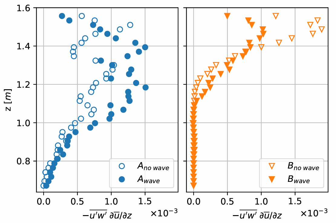
```latexP=-\left(\overline{u^{\prime}u^{\prime}}\frac{\partial\overline{u}}{\partial x}+\overline{w^{\prime}w^{\prime}}\frac{\partial\overline{w}}{\partial z}+\overline{u^{\prime}w^{\prime}}\frac{\partial\overline{u}}{\partial z}+\overline{u^{\prime}w^{\prime}}\frac{\partial\overline{w}}{\partial x}\right)```

(5)

Figure 17 presents the vertical profile of turbulent dissipation $$- \overline{u^{\prime} w^{\prime}} \frac{\partial \overline{u}}{\partial z}$$, which is the dominant term in both $$A$$ and $$B$$ cases. The spatial derivatives are calculated using a second-order centred finite difference scheme. Without waves, the production of TKE is maximal at the area corresponding to the passage of large-scale flow structures [51]. This occurs at $$z \geq 1 . 0$$ m for the $$A_{n o\, w a v e}$$ case and at $$z \geq 1 . 4$$ m for the $$B_{n o \,w a v e}$$ case, as expected. The effect of the wave direction is clearly evident. For waves with current ($$A_{w a v e}$$ case), the production increases at $$z \geq 1 . 0$$ m, while for wave against current ($$B_{w a v e}$$ case), a decrease is observed at $$z \geq 1 . 4$$ m. This is directly related to the increase in the velocity gradient observed previously (see Figure 12, $$A_{w a v e}$$ case) and the decrease in $$\overline{u^{\prime} w^{\prime}}$$ while maintaining a similar velocity gradient (see Figure 13, $$B_{w a v e}$$ case). For the present flow configuration, with a negative axial velocity gradient $$\frac{\partial \overline{u}}{\partial z} < 0$$, the vertical mixing and associated kinetic energy production appear to be enhanced in presence of waves following the current. This is directly related to the sign of the vertical gradient of the wave orbital velocity, which is of opposite sign of the current one.

Figure 17. Vertical profiles of the main contribution of the production of turbulent kinetic energy $$-\overline{u^{\prime}w^{\prime}}\frac{\partial\overline{u}}{\partial z}$$ for both $$A$$ and $$B$$ cases with waves (filled markers) and with no wave (empty markers).

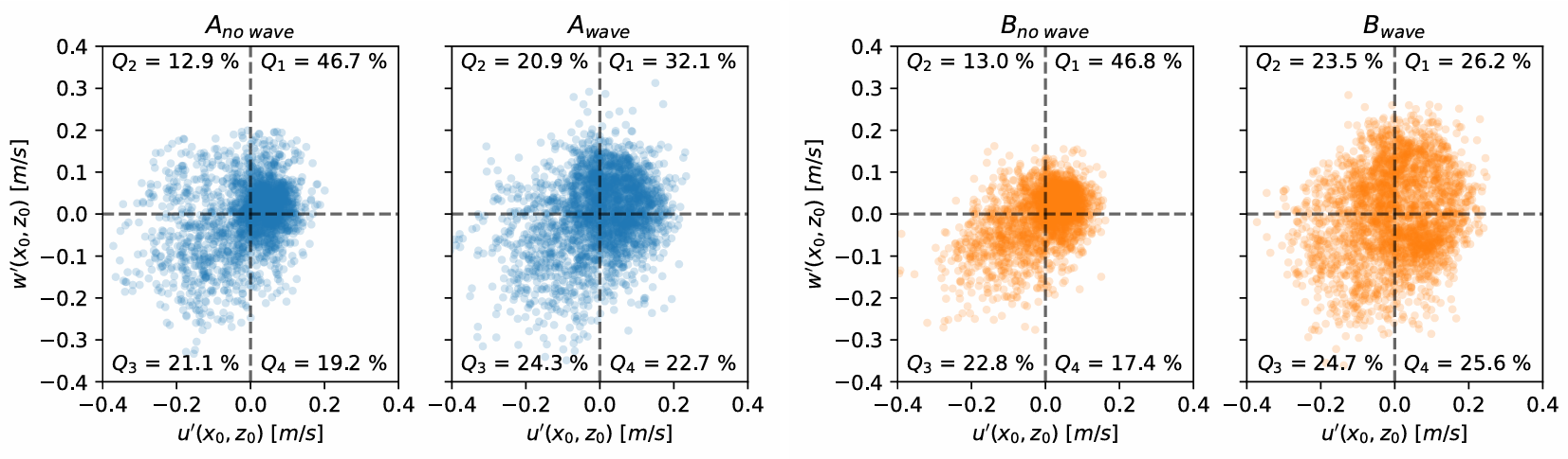
5.7. Quadrant Analysis A preliminary attempt to understand the physics of generating Reynolds shear stresses is made by performing a quadrant analysis [53]. This analysis also enables the nature of the organised flow structures in turbulent shear flows to be accessed [54]. The instantaneous contribution of velocity fluctuations $$u^{\prime}$$ and $$w^{\prime}$$ are sorted into four quadrants, denoted $$\left( Q_{1} , Q_{2} , Q_{3} , Q_{4} \right)$$, related to sweep and/or ejection events. An illustration of this is shown in Figure 18, based on velocity measurements in $$A$$ and $$B$$ cases. In these figures, the quadrant analysis is conducted using instantaneous fluctuating velocities extracted at $$x_{0}$$ and at a depth corresponding to $$z_{0}$$, where flow structures are present. Since the mean velocity vertical gradient $$\frac{\partial \overline{u}}{\partial z}$$ is negative in each case, the events in $$Q_{1}$$ and $$Q_{3}$$ are the main contributors to the Reynolds stresses. Conversely, in the presence of waves, regardless of their direction, the strong vertical velocity fluctuations coming from the wave surface significantly alter the nature of the organised flow structures. This effect is even more pronounced when waves propagate against the current, where it is observed that events in each $$Q$$ contribute almost equally to the Reynolds stress. 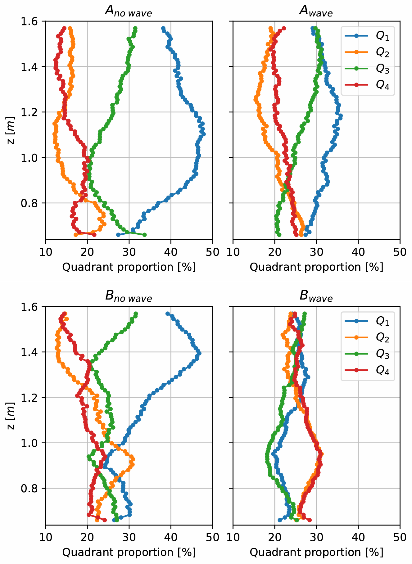Figure 19 presents the vertical profile of the quadrant proportion in each case. The presence of waves clearly impacts the instantaneous organisation of the flow by decreasing the events in $$Q_{1}$$ and simultaneously by increasing the events in $$Q_{2}$$ and $$Q_{4}$$. This analysis needs to be further performed by using a method that properly separates waves from turbulence to better emphasise the dynamics of the wave-turbulence interaction.

Figure 18. Quadrant analysis based on instantaneous fluctuating velocities $$\left( u^{\prime} , w^{\prime} \right)$$, extracted at $$x_{0} = - 0 . 2$$ m and $$z_{0} = 1 . 0$$ m for $$A$$ cases and $$z_{0} = 1 . 4$$ m for $$B$$ cases.

Figure 19. Evolution of the proportions (expressed in percentage values) of each quadrant event along the vertical line located at $$x_{0}$$, for $$A$$ cases (top) and $$B$$ cases (bottom).

6. Conclusions

A better understanding of wave interactions with turbulent flow in the water column is crucial for ocean sciences. This is because the induced turbulent processes impact ocean vertical mixing and energy transfer, which are of great interest not only for defining the future area for tidal energy converters but also for characterising the hydrodynamic loads exerted on marine structures, such as offshore wind turbine foundations and masts. The distribution of the vertical mean flow field and its associated turbulence is rarely uniform in the water column. In tidal flow, large-scale flow structures are often present, mainly originated from the bathymetry bed floor or anthropogenic actions. Therefore, this experimental work aims to study the wave effects on these convected flow structures by comparing the complex and turbulent flow characteristics without waves to those with waves following and opposing a positively sheared current. Based on wave gauges and PIV measurements, several processing tools are used to extract the main parameters of the flow characteristics. Results are summarised and discussed below.

: The mean velocity flow is slightly impacted by waves, although the mean axial velocity is more reduced near the water surface when waves propagate with the current than against it. Additionally, the vertical shear of the axial velocity is slightly modified. The mean vertical velocity shows some vertical oscillations directly related to the fixed wave frequency.
: The Turbulent Kinetic Energy increases in the water column for current and wave cases, comparing to current-only cases. This effect is more pronounced when waves propagate against the current. Without waves, the largest values of the shear stress Reynolds tensor component, $$\overline{u^{\prime} w^{\prime}}$$, occur at the depth correspond-ing to the passage of the large-scale flow structures. However, with waves, these maximum values are reduced, regardless of the wave’s direction.
: The PSD analysis highlights that the low frequency associated with the large-scale flow structures is slightly altered in presence of waves. Furthermore, the energy content of these flow structures increases in the water column, as previously noted. Additionally, these structures are detected over a greater vertical extent compared to the turbulent current-only cases. However, further confirmation is needed by considering other wave characteristics, such as various frequencies and amplitudes.
: The integral time scale, also known as the integral axial scale, is one of the characteristics most affected by the waves, regardless of their propagation direction. Waves significantly modify the instantaneous axial velocity fluctuations, reducing the temporal coherence of the velocity field.
: The presence of waves, either with or against the current, significantly alters the Probability Density Functions of fluctuating velocity fields compared to the PDFs of current-only cases. More specifically, when waves propagate against the current, a bimodal PDF representation is obtained, which greatly deviates from a Gaussian representation.
: The Turbulent Kinetic Energy production is modified as a function of the wave propagation direction. It notably increases for waves following the current. This is because the vertical velocity gradients associated with the current and the wave orbital velocity are of opposite sign.
: A preliminary quadrant analysis has shown that waves significantly impact flow organisation, particularly when waves propagate against the current.

In conclusion, the effects of wave on large-scale turbulent flow structures have been clearly demonstrated in the water column. These effects primarily impact turbulence levels, integral time scales, flow Gaussianity, and turbulence enhancement. Additionally, they are related to the vertical gradient of the current, which is linked to the wave orbital velocities. The present results enhance our understanding of wave-current interactions in the presence of large-scale energetic structures. However, further studies are required to fully understand the relevant mechanisms of nonlinear wave-current interactions. This includes conducting more test cases with various wave amplitudes and frequencies, as well as exploring irregular waves. Furthermore, future works should focus on extracting the wave field from raw velocity databases to provide a new perspective on the dynamics of wave-vortex interactions.

Statement of the Use of Generative AI and AI-Assisted Technologies in the Writing Process

The authors didn’t use AI tools to writing this manuscript nor processing the data.

Acknowledgments

The authors acknowledge Jean-Valéry Facq, Benoît Gomez and Nabila Ahssayni for their help during the tests.

Author Contributions

Conceptualization, P.D. and B.G.; Methodology, P.D. and B.G.; Validation, G.G., P.D. and B.G.; Formal Analysis, P.D. and B.G.; Investigation, P.D. and B.G.; Resources, B.G. and G.G.; Data Curation, B.G.; Writing—Original Draft Preparation, P.D.; Writing—Review & Editing, B.G. and G.G.; Visualization, B.G.; Supervision, G.G. and P.D.; Project Administration, G.G. and B.G.; Funding Acquisition, G.G. and B.G.

Ethics Statement

Not applicable.

Informed Consent Statement

Not applicable.

Data Availability Statement

The data supporting the findings of this study are available from the corresponding author, upon reasonable request.

Funding

Declaration of Competing Interest

The authors declare that they have no known competing financial interests or personal relationships that could have appeared to influence the work reported in this paper.

References

Perez L, Cossu R, Grinham A, Penesis I. Seasonality of turbulence characteristics and wave-current interaction in two prospective tidal energy sites. Renew. Energy 2021, 178, 1322–1336. doi:10.1016/j.renene.2021.06.116. [Google Scholar]

Yang Y, Stansby PK, Rogers BD, Buldakov E, Stagonas D, Draycott S. The loading on a vertical cylinder in steep and breaking waves on sheared currents using smoothed particle hydrodynamics. Phys. Fluids 2023, 35, 087132. doi:10.1063/5.0160021. [Google Scholar]

Bai H, Xu K, Zhang M, Yuan W, Jin R, Li W, et al. Theoretical and experimental study of the high-frequency nonlinear dynamic response of a 10 MW semi-submersible floating offshore wind turbine. Renew. Energy 2024, 231, 120952. doi:10.1016/j.renene.2024.120952. [Google Scholar]

Hubert Z, Louchart AP, Robache K, Epinoux A, Gallot C, Cornille V, et al. Decadal changes in phytoplankton functional composition in the Eastern English Channel: Possible upcoming major effects of climate change. Ocean Sci. 2025, 21, 679–700. doi:10.5194/os-21-679-2025. [Google Scholar]

Denman KL, Gargett AE. Time and space scales of vertical mixing and advection of phytoplankton in the upper ocean. Limnol. Oceanogr. 1983, 28, 801–815. doi:10.4319/lo.1983.28.5.0801. [Google Scholar]

Qiao F, Yuan Y, Deng J, Dai D, Song Z. Wave–turbulence interaction-induced vertical mixing and its effects in ocean and climate models. Philos. Trans. R. Soc. A Math. Phys. Eng. Sci. 2016, 374, 20150201. doi:10.1098/rsta.2015.0201. [Google Scholar]

Mercier P, Guillou S. The impact of the seabed morphology on turbulence generation in a strong tidal stream. Phys. Fluids 2021, 33, 055125. doi:10.1063/5.0047791. [Google Scholar]

Ikhennicheu M, Germain G, Druault P, Gaurier B. Experimental study of coherent flow structures past a wall-mounted square cylinder. Ocean Eng. 2019, 182, 137–146. doi:10.1016/j.oceaneng.2019.04.043. [Google Scholar]

Mercier P, Ikhennicheu M, Guillou S, Germain G, Poizot E, Grondeau M, et al. The merging of Kelvin–Helmholtz vortices into large coherent flow structures in a high Reynolds number flow past a wall-mounted square cylinder. Ocean Eng. 2020, 204, 107274. doi:10.1016/j.oceaneng.2020.107274. [Google Scholar]

10.

Blackmore T, Myers LE, Bahaj AS. Effects of turbulence on tidal turbines: Implications to performance, blade loads, and condition monitoring. Int. J. Mar. Energy 2016, 14, 1–26. doi:10.1016/j.ijome.2016.04.017. [Google Scholar]

11.

Druault P, Germain G. Prediction of the tidal turbine power fluctuations from the knowledge of incoming flow structures. Ocean Eng. 2022, 252, 111180. doi:10.1016/j.oceaneng.2022.111180. [Google Scholar]

12.

Druault P, Gaurier B, Germain G. Impact of varying turbulent flow conditions on the tidal turbine blade load fatigue. Renew. Energy 2025, 251, 123370. doi:10.1016/j.renene.2025.123370. [Google Scholar]

13.

McWilliams JC. Submesoscale currents in the ocean. Proc. R. Soc. A Math. Phys. Eng. Sci. 2016, 472, 20160117. doi:10.1098/rspa.2016.0117. [Google Scholar]

14.

Smeltzer BK, Rømcke O, Hearst RJ, Ellingsen A. Experimental study of the mutual interactions between waves and tailored turbulence. J. Fluid Mech. 2023, 962, R1. doi:10.1017/jfm.2023.280. [Google Scholar]

15.

Soulsby R, Hamm L, Klopman G, Myrhaug D, Simons R, Thomas G. Wave-current interaction within and outside the bottom boundary layer. Coast. Eng. 1993, 21, 41–69. doi:1016/0378-3839(93)90045-A. [Google Scholar]

16.

Zhang X, Simons R, Zheng J, Zhang C. A review of the state of research on wave-current interaction in nearshore areas. Ocean Eng. 2022, 243, 110202. doi:10.1016/j.oceaneng.2021.110202. [Google Scholar]

17.

Zhang J-S, Zhang Y, Jeng D-S, Liu P-F, Zhang C. Numerical simulation of wave–current interaction using a RANS solver. Ocean Eng. 2014, 75, 157–164. doi:10.1016/j.oceaneng.2013.10.014. [Google Scholar]

18.

Sentchev A, Nguyen TD, Furgerot L, Bailly du Bois P. Underway velocity measurements in the Alderney Race: Towards a three-dimensional representation of tidal motions. Philos. Trans. R. Soc. A Math. Phys. Eng. Sci. 2020, 378, 20190491. doi:10.1098/rsta.2019.0491. [Google Scholar]

19.

Bennis A-C, Furgerot L, Bailly du Bois P, Dumas F, Odaka T, Lathuili C, et al. Numerical modelling of three-dimensional wave-current interactions in complex environment: Application to Alderney Race. Appl. Ocean Res. 2020, 95, 102021. doi:10.1016/j.apor.2019.102021. [Google Scholar]

20.

Mohapatra SC, Amouzadrad P, Bispo IBDS, Soares CG. Hydrodynamic Response to Current and Wind on a Large Floating Interconnected Structure. J. Mar. Sci. Eng. 2025, 13, 63. doi:10.3390/jmse13010063. [Google Scholar]

21.

Rahman A, Farrok O, Haque MM. Environmental impact of renewable energy source based electrical power plants: Solar, wind, hydroelectric, biomass, geothermal, tidal, ocean, and osmotic. Renew. Sustain. Energy Rev. 2022, 161, 112279. doi:10.1016/j.rser.2022.112279. [Google Scholar]

22.

Roy S, Samantaray SS, Debnath K. Study of turbulent eddies for wave against current. Ocean Eng. 2018, 150, 176–193. doi:10.1016/j.oceaneng.2017.12.059. [Google Scholar]

23.

Roy S, Debnath K, Mazumder BS. Distribution of eddy scales for wave current combined flow. Appl. Ocean Res. 2017, 63, 170–183. doi:10.1016/j.apor.2017.01.005. [Google Scholar]

24.

Magnier M, Gaurier B, Germain G, Druault P. Analysis of the wake of a wide bottom-mounted obstacle in presence of surface wave following tidal current. In Trends in Renewable Energies Offshore, 1st ed.; CRC Press: Boca Raton, FL, USA, 2022. doi:10.1201/9781003360773-18.

25.

Saouli Y, Magnier M, Germain G, Gaurier B, Druault P. Experimental Characterisation of the Wave Propagating Against Current Effects on the Wake of a Wide Bathymetric Obstacle. In Proceedings of the JH2022-18`emes Journ´ees de l’Hydrodynamique, Poitiers, France, 22–24 Novembre 2022.

26.

Magnier M, Saouli Y, Gaurier B, Druault P, Germain G. Modification of the wake of a wall-mounted bathymetry obstacle submitted to waves opposing a tidal current. Ocean Eng. 2023, 288, 116087. doi:10.1016/j.oceaneng.2023.116087. [Google Scholar]

27.

Ouro P, Mullings H, Christou A, Draycott S, Stallard T. Wake characteristics behind a tidal turbine with surface waves in turbulent flow analyzed with large-eddy simulation. Phys. Rev. Fluids 2024, 9, 034608. doi:10.1103/PhysRevFluids.9.034608. [Google Scholar]

28.

Zhang Z, Zhang Y, Zheng Y, Zhang J, Fernandez-Rodriguez E, Zang W, et al. Power fluctuation and wake characteristics of tidal stream turbine subjected to wave and current interaction. Energy 2023, 264, 126185. doi:10.1016/j.energy.2022.126185. [Google Scholar]

29.

Zhang Y, Zhang Z, Zheng J, Zhang J, Zheng Y, Zang W, et al. Experimental investigation into effects of boundary proximity and blockage on horizontal-axis tidal turbine wake. Ocean Eng. 2021, 225, 108829. doi:10.1016/j.oceaneng.2021.108829. [Google Scholar]

30.

Gaurier B, Germain G, Facq JV, Bacchetti T. Wave and Current Flume Tank of Boulogne-sur-Mer, Description of the Facility and Its Equipment ; IFREMER: Boulogne-Sur-Mer, France, 2018. doi:10.13155/58163.

31.

Edinburgh Designs. Piston Coastal Wave Generators. 2025. Available online: http://www4.edesign.co.uk/product/piston- wave-generators/ (accessed on 21 December 2025).

32.

Gaurier B, Bacchetti T, Facq JV, Germain G. Essais Combin´es Houle-Courant: Caract´erisation des Conditions G´en´er´ees au Bassin de Boulogne-sur-Mer ; IFREMER: Boulogne-Sur-Mer, France, 2010.

33.

Le Boulluec M, Kimmoun O, Molin B. Etude Exp´erimentale Pour l’Optimisation des Performances d’une Plage d’Amortissement Parabolique. In Proceedings of the 11`emes Journ´ees de l’Hydrodynamique, Brest, France, 3–5 April 2007. Available online: https://archimer.ifremer.fr/doc/00170/28170/ (accessed on 21 December 2025).

34.

Furgerot L, Sentchev A, Bailly du Bois P, Lopez G, Morillon M, Poizot E, et al. One year of measurements in Alderney Race: Preliminary results from database analysis. Philos. Trans. R. Soc. A Math. Phys. Eng. Sci. 2020, 378, 20190625. doi:10.1098/rsta.2019.0625. [Google Scholar]

35.

Ikhennicheu M. Étude Expérimentale de la Turbulence dans les Zones à Forts Courants et de son Impact sur les Hydroliennes. Ph.D. Thesis, Université de Lille, Lille, France, 2019.

36.

Ahmed U, Apsley D, Afgan I, Stallard T, Stansby P. Fluctuating loads on a tidal turbine due to velocity shear and turbulence: Comparison of CFD with field data. Renew. Energy 2017, 112, 235–246. doi:10.1016/j.renene.2017.05.048. [Google Scholar]

37.

Mullings H, Stallard T. Impact of spatially varying flow conditions on the prediction of fatigue loads of a tidal turbine. Int. Mar. Energy J. 2022, 5, 103–111. doi:10.36688/imej.5.103-111. [Google Scholar]

38.

Wang P, Li K, Wang L, Huang B. Generation and distribution of turbulence-induced loads fluctuation of the horizontal axis tidal turbine blades. Phys. Fluids 2024, 36, 015151. doi:10.1063/5.0186105. [Google Scholar]

39.

Gaurier B, Ikhennicheu M, Germain G, Druault P. Experimental study of bathymetry generated turbulence on tidal turbine behaviour. Renew. Energy 2020, 156, 1158–1170. doi:10.1016/j.renene.2020.04.102. [Google Scholar]

40.

Stanislawski BJ, Thedin R, Sharma A, Branlard E, Vijayakumar G, Sprague MA. Effect of the integral length scales of turbulent inflows on wind turbine loads. Renew. Energy 2023, 217, 119218. doi:10.1016/j.renene.2023.119218. [Google Scholar]

41.

Schottler J, Reinke N, Hölling A, Whale J, Peinke J, Hölling M. On the impact of non-Gaussian wind statistics on wind turbines—An experimental approach. Wind Energy Sci. 2017, 2, 1–13. doi:10.5194/wes-2-1-2017. [Google Scholar]

42.

Welch P. The use of fast Fourier transform for the estimation of power spectra: A method based on time averaging over short, modified periodograms. IEEE Trans. Audio Electroacoust. 1967, 15, 70–73. doi:1109/TAU.1967.1161901. [Google Scholar]

43.

Virtanen P, Gommers R, Oliphant TE, Haberland M, Reddy T, Cournapeau D, et al. SciPy 1.0: Fundamental algorithms for scientific computing in Python. Nat. Methods 2020, 17, 261–272. doi:10.1038/s41592-019-0686-2. [Google Scholar]

44.

Omidyeganeh M, Piomelli U. Large-eddy simulation of two-dimensional dunes in a steady, unidirectional flow. J. Turbul. 2011, 12, N42. doi:10.1080/14685248.2011.609820. [Google Scholar]

45.

Druault P, Gaurier B, Germain G. Spatial integration effect on velocity spectrum: Towards an interpretation of the–11/3 power law observed in the spectra of turbine outputs. Renew. Energy 2022, 181, 1062–1080. doi:10.1016/j.renene.2021.09.106. [Google Scholar]

46.

Wolf J, Prandle D. Some observations of wave–current interaction. Coast. Eng. 1999, 37, 471–485. doi:10.1016/S0378-3839(99)00039-3. [Google Scholar]

47.

Dean RG, Dalrymple RA. Water Wave Mechanics for Engineers and Scientists. World Sci. 1991, 2, 368. doi:10.1142/1232. [Google Scholar]

48.

Nielsen P, You Z-J. Eulerian Mean Velocities Under Non-Breaking Waves on Horizontal Bottoms. Coast. Eng. 1996, 4066–4078. doi:10.1061/9780784402429.314. [Google Scholar]

49.

Olabarrieta M, Medina R, Castanedo S. Effects of wave–current interaction on the current profile. Coast. Eng. 2010, 57, 643–655. doi:10.1016/j.coastaleng.2010.02.003. [Google Scholar]

50.

Mazumder B, Ojha SP. Turbulence statistics of flow due to wave–current interaction. Flow Meas. Instrum. 2007, 18, 129–138. doi:10.1016/j.flowmeasinst.2007.05.001. [Google Scholar]

51.

Ikhennicheu M, Druault P, Gaurier B, Germain G. Turbulent kinetic energy budget in a wall-mounted cylinder wake using PIV measurements. Ocean Eng. 2020, 210, 107582. doi:1016/j.oceaneng.2020.107582. [Google Scholar]

52.

Magnier M, Druault P, Germain G. Experimental investigation of upstream cube effects on the wake of a wall-mounted cylinder: Wake rising reduction, TKE budget and flow organization. Eur. J. Mech. B/Fluids 2021, 87, 92–102. doi:10.1016/j.euromechflu.2021.01.004. [Google Scholar]

53.

Antonia RA, Browne LWB. Quadrant analysis in the turbulent far-wake of a cylinder. Fluid Dyn. Res. 1987, 2, 3–14. doi:10.1016/0169-5983(87)90013-X. [Google Scholar]

54.

Wallace JM. Quadrant Analysis in Turbulence Research: History and Evolution. Annu. Rev. Fluid Mech. 2016, 48, 131–158. doi:10.1146/annurev-fluid-122414-034550. [Google Scholar]