Binocular Camera-Based Depth Recognition for Motion Monitoring and Response Analysis of Flexible Floating Structures for Offshore Photovoltaics

With the continuous growth of global electricity demand and the extensive consumption of fossil fuels, and as the challenges posed by climate change and the increasing frequency of extreme weather events continue to intensify, the development of clean and renewable energy has become an urgent priority [1,2,3]. However, the rigid land requirements of ground-based photovoltaic (PV) projects have become a major bottleneck restricting their large-scale deployment [4]. As a highly promising solution, offshore floating photovoltaic (OFPV) power plants deploy PV modules on the water surface using floating structures, not only conserving valuable land resources but also making full use of the abundant solar energy available at sea [5]. In recent years, offshore floating photovoltaic (OFPV) systems have gradually become a research focus in both academia and industry [6]. Companies such as Ocean Sun (Norway), Oceans of Energy (The Netherlands), as well as China Resources Power, State Power Investment Corporation, and China National Offshore Oil Corporation have established demonstration projects in locations including the Philippines, the North Sea, Dong ying, the Bohai Sea in Tianjin, and the Shandong Peninsula [7,8].

Currently, offshore photovoltaic (PV) technology is mainly classified into two categories: fixed and floating systems [9]. Among them, floating systems offer significant advantages: they do not require pile foundations, substantially reducing steel consumption and construction costs, while also avoiding disturbances to nearshore ecosystems [10]. In addition, they can be deployed in areas with water depths of 5 m or more and withstand wave forces, thereby increasing installed capacity per unit area by over 20% [11]. Moreover, the natural cooling effect of seawater can lower module temperatures by 5–8 °C, thereby increasing photovoltaic conversion efficiency by 12–13% [12,13,14]. The mobility and upgradability of floating photovoltaic systems can also extend their service life, providing a “zero ecological impact” solution that combines technological, economic, and environmental benefits. At the same time, by reducing excessive photosynthesis and algal growth, they contribute to improving water quality [15,16,17]. Nonetheless, floating systems still face numerous challenges in acquiring motion response data and ensuring structural safety. Therefore, research on accurate motion measurement and tracking of floating bodies holds significant engineering and scientific value.

Measurement and tracking methods can generally be classified into two categories: contact and non-contact approaches. Traditional contact-based methods rely on rulers, potentiometers, and gyroscopes to manually record the motion states of floating structures [18,19]. Such methods are not only labor-intensive and lack real-time capability, but also often fail to meet the precision requirements of experiments. In recent years, sensor systems composed of accelerometers, gyroscopes, and orientation sensors have been developed to measure instantaneous acceleration and angular position at a given point, with displacement estimated through integration of the acceleration data [20,21,22]. However, such systems are prone to drift errors during long-term monitoring, which can significantly compromise data accuracy. Moreover, offshore floating photovoltaic (OFPV) systems are typically composed of a ring frame and an internal thin film, and the weight of contact sensors can interfere with the natural motion response of the film, thereby limiting measurement accuracy.

Non-contact visual recognition technologies have attracted increasing attention due to their high accuracy, low cost, ease of deployment, and long-distance monitoring capabilities [23]. Visual tracking methods are generally classified into two types: monocular and binocular approaches. Although monocular systems can capture two-dimensional features using a single camera, they cannot directly obtain depth information and are prone to cumulative estimation errors [24]. In contrast, binocular vision mimics the human stereoscopic perception mechanism and can achieve real-time 3D scene reconstruction without prior size information, offering both compact structure and high accuracy [25,26]. However, conventional binocular algorithms require substantial computational resources for feature matching and disparity calculation. In marine environments, strong reflections from the water surface and weak texture features can degrade performance, resulting in unstable depth estimation [27,28].

In recent years, binocular vision–based systems for marine and underwater applications have achieved significant progress. For example, binocular stereo vision has been applied to underwater target detection and ranging, measurement of underwater object dimensions, and identification of defects in underwater pile concrete [29,30,31]. Beyond the field of construction, further studies in agriculture and biological monitoring have also demonstrated its effectiveness in positioning and target recognition [32,33,34]. In addition, binocular vision has been employed for road pothole detection, robot navigation, and real-time 3D reconstruction for robots [35,36,37].

These advances indicate that the simultaneous implementation of motion tracking and stereoscopic information acquisition has become one of the core capabilities of modern machine vision technologies. Binocular depth cameras, with their compact structure and mobility, are particularly suitable for dynamic monitoring of floating engineering structures, offering a highly promising solution for motion tracking and measurement of floating bodies in real marine environments [38,39]. The remainder of this paper is organized as follows: Section 2 provides a detailed description of the experimental site, the physical model, the overall observation system, and the corresponding test conditions. Section 3 explains the working principles of the binocular depth camera used in the experiments, including its technical specifications and relevant mathematical formulations. Section 4 presents the validation and comparative evaluation of the proposed monitoring method, and analyzes the effects of different test conditions on the dynamic response of the model. Finally, Section 5 summarizes the main findings and conclusions of this study.

The experiments were conducted in the harbor basin of a key laboratory at Tianjin University. The harbor basin measures 60 m × 15 m × 1.5 m (length × width × depth), with a maximum effective water depth of 0.6 m. Ten wave generators are installed along one side of the basin, of which six were activated in this study. These wave generators can produce both regular and irregular waves, with adjustable wave periods and heights, covering a wave period range from 0.5 s to 5.0 s. To suppress wave reflections, the remaining boundaries of the basin are equipped with breakwaters and wave-absorbing materials.

The experimental model was fabricated from high-density polyethylene (HDPE) and primarily consists of three components: a breakwater plate, a float box, and side plates. The breakwater plate is arranged in two concentric layers on both sides of the structure, designed to attenuate incident wave forces. The float box serves as the primary buoyant component, while the side plates enable modular connection of smaller components.

The model represents a flexible thin-film floating system, comprising a floating ring, a thin-film structure, and a mooring system. The floating ring is assembled from eight arc-shaped units, each comprising a buoyancy chamber, a breakwater panel, and nine side plates. The buoyancy chamber provides flotation, the breakwater panel reduces wave loads, and the side plates ensure structural connection between adjacent units. The overall structure of the floating body model and the experimental setup are shown in Figure 1.

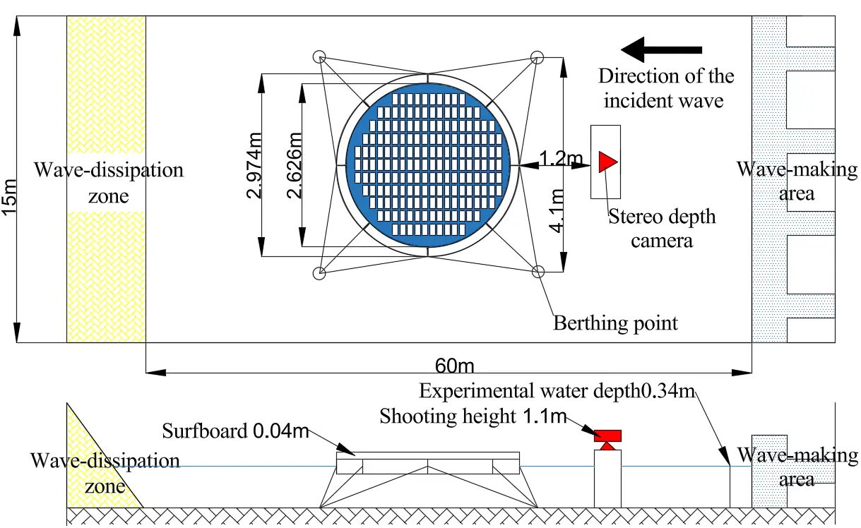
As shown in Figure 1, the experiments were conducted under a water depth of 0.34 m. The single-ring model has an outer diameter of 2.974 m and an inner diameter of 2.626 m, and is equipped with a 0.04 m high wave-guiding plate. The thin-film area is 21 m², and the model was designed according to a geometric similarity ratio of $$\lambda =1:50$$. To satisfy gravitational similarity, a total lead ballast of 2.4386 kg was added to the inner surface of the waterproof membrane, complemented by uniformly distributed weights to simulate the load of the photovoltaic panels. In addition, 32 iron ballast blocks (dimensions: 0.15 m × 0.025 m × 0.05 m; mass per block: 1.47 kg) were installed at the outer corners of the float box.

The mooring system consists of four anchors and twelve mooring chains, designed according to the principles of elastic similarity. Linear springs were connected in series along the mooring chains to simulate the linear variation characteristics of mooring stiffness. A total of twelve mooring lugs were installed at eight equally spaced positions along the outer circumference of the ring to connect the mooring chains. Motion tracking was performed using a binocular camera, positioned at a horizontal distance of 1.2 m from the model and mounted at a height of 1.1 m.

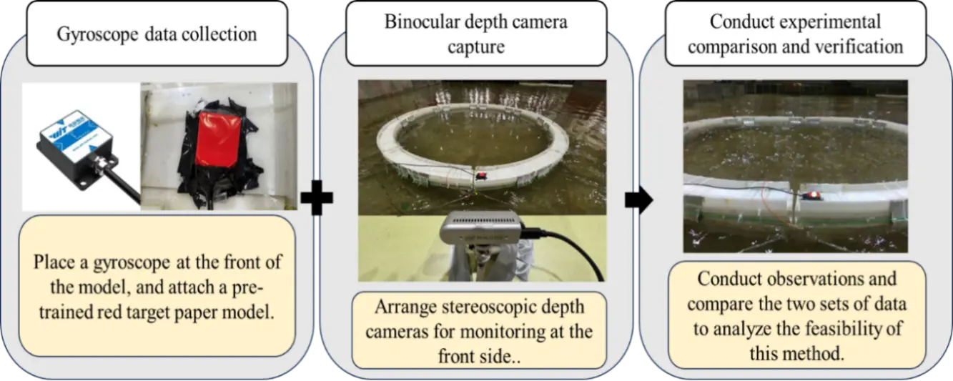
The flexible thin-film floating body tracking system, based on a deep learning-driven YOLOv8 algorithm and a stereo depth camera, follows the workflow illustrated in Figure 2.

As shown in Figure 2, the study established a real-time tracking framework by seamlessly integrating the YOLOv8 object detection network with a stereo depth camera system. The overall workflow can be divided into two main stages: model training and optimization, and three-dimensional coordinate reconstruction and tracking.

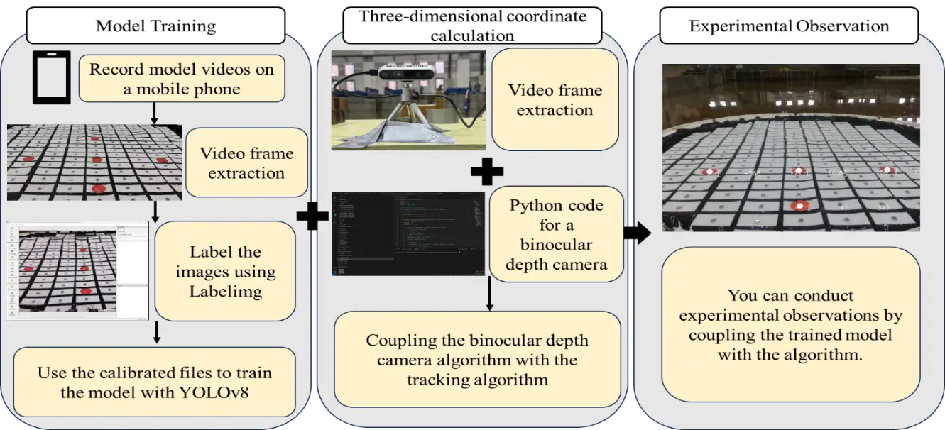
Model training. To construct a representative training dataset, video sequences of the experimental environment were first captured with a handheld imaging device under varying lighting and viewing angle conditions. Approximately 1000 frames were uniformly sampled from these sequences to maximize dataset diversity and completeness, ensuring that the trained model possesses strong generalization capability. Each frame was annotated using labeling tools, and the bounding box coordinates and class labels were carefully verified manually to ensure high annotation reliability. After dataset preparation, transfer learning was performed within the YOLOv8 framework, initializing the model with pre-trained weights to accelerate convergence and enhance robustness. During training, convergence was continuously monitored using cross-validation, F1 score, and mAP@0.5 metrics, and the weights achieving the best validation performance were selected as the final detection model for deployment.

For three-dimensional coordinate computation, the stereo image pairs were rectified and aligned in real time using the stereo camera SDK within a Python environment, and subsequently generated dense depth maps. The rectified RGB frames were processed by the trained YOLOv8 model to achieve stable object detection in dynamic scenes. Subsequently, using the camera intrinsic matrix, the centroids of each detected bounding box were back-projected along with their corresponding depth values to reconstruct three-dimensional spatial coordinates with millimeter-level accuracy. To reduce random fluctuations and suppress high-frequency noise, the reconstructed coordinate time series across consecutive frames was processed using a median filter. In addition, the Deep SORT algorithm was employed to assign globally unique tracking IDs, maintaining object identities and ensuring trajectory continuity even under partial occlusion or temporary detection loss.

By tightly coupling the detection and reconstruction stages, the proposed system demonstrates centimeter-level spatial localization accuracy with millisecond-level update rates. This capability not only enables accurate and real-time trajectory monitoring but also provides a high-quality data foundation for advanced tasks such as motion prediction, behavior recognition, and dynamic system analysis.

This study employed an integrated stereo depth camera, which, leveraging advanced stereo vision sensing technology, enables video capture, depth information acquisition, and real-time localization. When the stereo depth camera captures a target object, its two cameras simultaneously record images from different viewpoints. By analyzing the disparity between these two images, the three-dimensional spatial coordinates and distance of the target relative to the camera can be calculated. The stereo depth camera provides high-resolution, high-accuracy depth data over a wide range, making it suitable for various application scenarios, as illustrated in Figure 3.

As shown in Figure 3, the Intel RealSense D325i camera was selected as the core sensing device of the experimental framework, primarily due to its integrated stereo vision and depth perception capabilities. The active infrared stereo depth channel of the camera provides an absolute metric scale for the bounding boxes detected by YOLOv8, thereby enabling precise three-dimensional localization. The D325i camera outputs high-definition dense depth maps with a resolution of 1280 × 720 pixels at a frame rate of 30 frames per second, and an effective operating depth range from 0.16 m to 2.0 m. According to the manufacturer’s specifications and experimental verification, the root mean square (RMS) error of the D325i remains below 2%, ensuring high depth accuracy and frame-to-frame consistency. In addition to the depth data stream, the camera is capable of simultaneously outputting full HD RGB images at a resolution of 1920 × 1080 and a frame rate of 30 frames per second. Although these RGB images are not directly involved in the final 3D coordinate computation, their rich texture information plays a crucial role in enhancing stereo matching performance, particularly in texture-sparse regions.

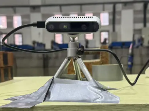
The D325i camera is equipped with an onboard D3 ASIC processor dedicated to real-time depth map computation, effectively offloading intensive processing tasks from the host CPU and GPU to reduce computational load. The RGB-D and MJPEG video streams are transmitted via a USB-C interface with minimal latency, allowing the system’s GPU to fully dedicate its resources to the YOLOv8-based object detection process and achieve optimal performance. In addition, the camera integrates a six-degree-of-freedom (6-DoF) inertial measurement unit (IMU), which, in combination with an external hardware trigger interface, enables timestamp synchronization with microsecond-level precision. This hardware-level timing control establishes a reliable foundation for subsequent spatiotemporal calibration and real-time motion compensation.

In summary, the Intel RealSense D325i camera, with its compact design, hardware-decoupled architecture, and high-precision depth sensing, serves as a stable, scalable data acquisition component within the YOLOv8 + depth 3D perception framework. It is suitable for real-time applications in dynamic, cluttered, or partially occluded environments.

The experimental water depth was set to 0.34 m, corresponding to a prototype depth of 17 m. To simulate irregular sea conditions, this study employed the JONSWAP spectrum and designed corresponding experimental scenarios: Under a fixed wave period, the acceleration of the floating body varies with different wave heights; conversely, under a fixed wave height, the acceleration changes with different wave periods. In the fixed wave period scenario, the wave period was set to 9.9 s, while the wave height was increased from 3 m to 6 m in 1 m increments. In the fixed wave height scenario, the wave height was maintained at 4 m, and the wave period was set successively to 6 s, 8 s, 9.9 s, and 12 s. The experiments were conducted at a geometric scale of 1:50, and the wave maker input parameters were calculated accordingly. The main experimental conditions are summarized in Table 1. Considering the symmetry of the flexible membrane and its mooring system, the wave incidence direction was fixed at 0°.

Four measurement points were arranged on the membrane, and the proposed method was employed to monitor these points. The specific layout of the measurement points is shown in Figure 4, while the experimental conditions are detailed in Table 1.

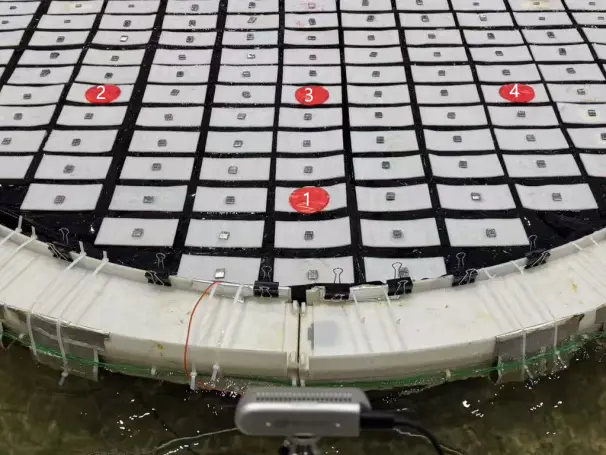
Among the measurement points, points 1 and 3 were used to analyze the characteristics during the forward and backward propagation of waves, while points 2, 3, and 4 were employed to examine whether wave attenuation differences occur along the same horizontal line under the given model conditions. For each test scenario, the measurement sampling interval was 0.0557 s, and approximately 1000 data points were collected over the 80-s test duration.

Stereo depth cameras have become a core sensing technology in the field of 3D perception. Their operating principle is based on geometric triangulation and can be rigorously derived using the classical pinhole camera model. By combining intrinsic and extrinsic parameters, the projection of 3D spatial points onto 2D image coordinates can be analytically described. Simultaneously, depth information can be inferred by estimating the disparity between stereo image pairs. This chapter presents the theoretical foundations of stereo imaging, including the pinhole projection model, the geometric relationships of stereo triangulation, coordinate transformations, and the back-projection mapping. These formulations establish the mathematical basis for subsequent applications in 3D reconstruction, object localization, and motion tracking under marine and engineering scenarios [39,40,41].

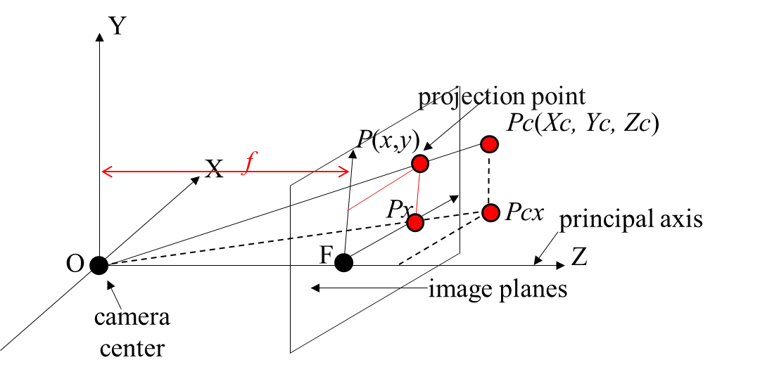
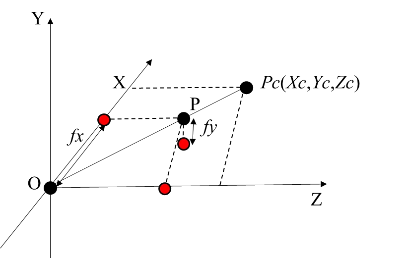
The binocular depth camera operates based on the principle of triangulation, and the classical pinhole camera formulation can rigorously model its imaging process. In this model, the camera is regarded as an ideal perspective projection system, where a spatial point $${P}_{c}\left({X}_{c},{Y}_{c},{Z}_{c}\right)$$ in the camera coordinate system is projected onto the image plane at $$P\left(x, y\right)$$. The projection depends on the intrinsic parameters of the camera (focal length, principal point, pixel scaling factors) and the extrinsic parameters (rotation and translation between the camera and world coordinate systems).

As illustrated in Figure 5, the pinhole camera model, widely adopted in computer vision and photogrammetry, assumes that the camera performs ideal perspective projection, in which three-dimensional points are mapped onto a two-dimensional image plane through an infinitesimally small aperture. The geometric interpretation of the projection is illustrated in Figure 5. The optical center $$O$$ is located at the origin of the camera coordinate system, and the principal axis is aligned with the Z-axis. The image plane is perpendicular to the principal axis and positioned at a distance $$f$$, where $$f$$ denotes the focal length. The intersection of the principal axis and the image plane defines the image center $$F$$. Based on the similarity of triangles △𝑂𝑃𝑃𝑥 and △𝑂𝑃𝑐𝑃𝑐𝑥, the fundamental projection equations can be derived as:

Here, $$\left({X}_{c},{Y}_{c},{Z}_{c}\right)$$ denote the 3D coordinates of a spatial point P in the camera coordinate system, and $$\left(x, y\right)$$ are the corresponding image-plane coordinates. $$f$$ represents the focal length of the camera. Equation (2) thus establishes the mapping between 3D spatial coordinates and 2D image coordinates under an ideal perspective projection without lens distortion.

To clearly illustrate the geometric relationship between different coordinate systems involved in the imaging process, Figure 6 presents the transformation from the image coordinate system to the pixel coordinate system.

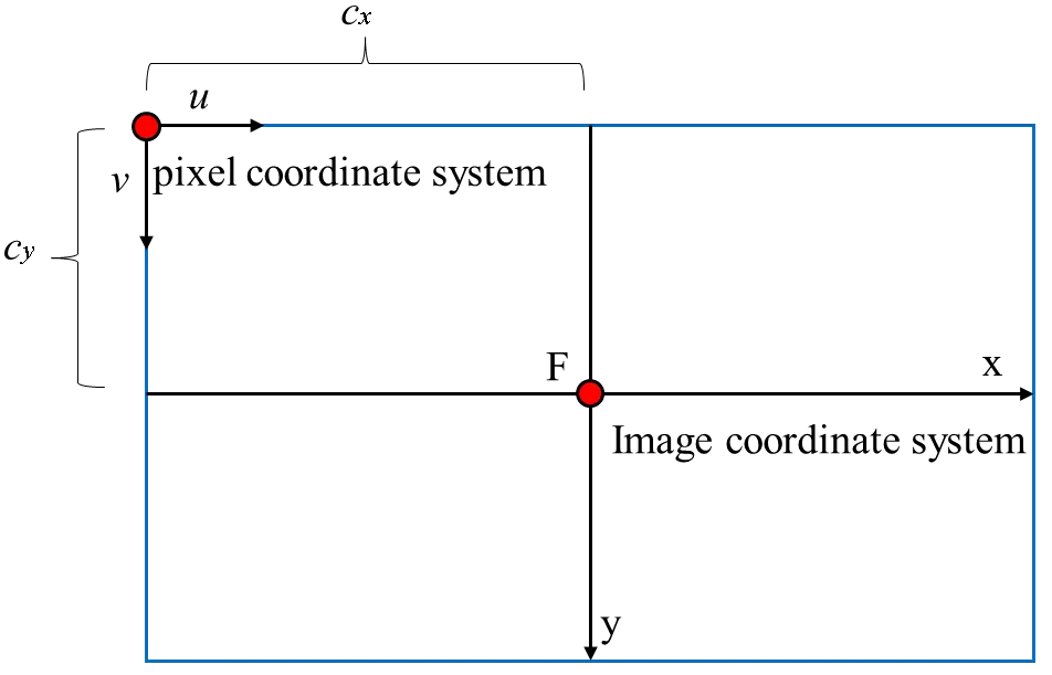
As illustrated in Figure 6, the image coordinate system $$\left(x, y\right)$$ is transformed into the pixel coordinate system $$\left(u, v\right)$$ to match actual pixel measurements. This transformation involves both translation and scaling, and is expressed as:

where $$\left({c}_{x},{c}_{y}\right)$$ denotes the principal point in the pixel coordinate system (i.e., the image center), $$\alpha$$ and $$\beta$$ are the horizontal and vertical scaling factors, respectively, which convert physical distances on the image plane into pixel units. Combining Equation (2) and Equation (3), the overall imaging process from a spatial point in the camera coordinate system to the pixel coordinate system can be represented in matrix form as:

To describe the mapping from the world coordinate system $$\left({X}_{w},{Y}_{w},{Z}_{w}\right)$$ to the pixel coordinate system $$\left(u, v\right)$$, the extrinsic parameters are introduced to represent the transformation between the world and camera coordinate systems. Accordingly, the complete imaging model can be expressed as:

where $$s$$ is a nonzero scale factor, $$K$$ denotes the intrinsic parameter matrix of the camera that incorporates the focal length and pixel scaling factors, $$R\in {R}^{3×3}$$ represents the rotation of the world coordinate system relative to the camera, and $$t\in {R}^{3×1}$$ denotes the translation vector. Equation (5) establishes the complete geometric relationship between the three-dimensional world coordinates and the two-dimensional pixel coordinates, providing the mathematical foundation for binocular vision and three-dimensional reconstruction.

Stereo depth cameras employ the principle of triangulation, where disparity information is obtained by matching images captured simultaneously by the left and right cameras, and, combined with intrinsic and extrinsic parameters, back-projection is performed to reconstruct the three-dimensional coordinates of scene pixels.

As illustrated in Figure 7, a typical stereo vision geometry can be described under the assumption of a parallel binocular configuration with perspective projection. Two horizontally aligned cameras (denoted as camera L and camera R) form a baseline system, where the distance between the two optical centers is the baseline length b, a critical parameter for disparity computation. Each camera has an image plane (depicted as black lines perpendicular to the optical axes), and the distance from the optical center to the image plane corresponds to the focal length $$f$$. A spatial point P (approximated as $$\left(x, z\right)$$ in the simplified camera coordinate system) is projected onto the left and right image planes at coordinates $${x}_{l}$$ and $${x}_{r}$$, respectively, via optical rays passing through the two camera centers.

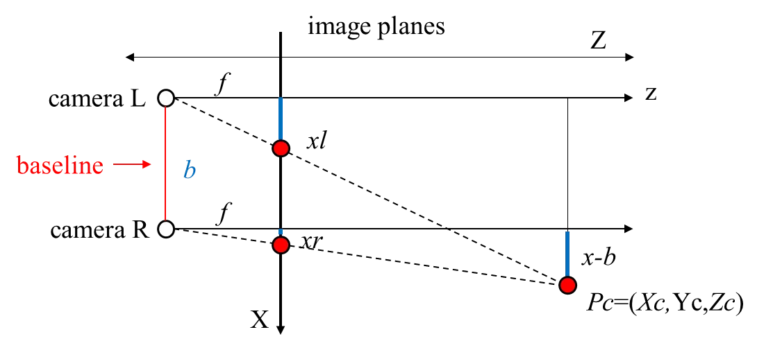
For the left camera, the optical center, point P, and the projection $${x}_{l}$$ form similar triangles, yielding the relationship

which can be rearranged to solve for $$z$$ (the depth):

Similarly, for the right camera, point $$P$$, the optical center, and the projection $${x}_{r}$$ Satisfy:

Combining Equation (7), Equation (8) and Equation (9) gives the fundamental depth–disparity relationship:

where $$d={x}_{l}-{x}_{r}$$ denotes the disparity between corresponding image points in the left and right views. In this formulation, $$f$$ represents the focal length of the camera, $$b$$ the baseline length (i.e., the distance between the optical centers of the two cameras), $$\left({x}_{l},{y}_{l}\right)$$ and $$\left({x}_{r},{y}_{r}\right)$$ the pixel coordinates of the same spatial point projected on the left and right image planes, $$P\left({X}_{w},{Y}_{w},{Z}_{w}\right)$$the world coordinates of the corresponding point in three-dimensional space, and $$Z$$ the depth of that point from the camera plane. This geometric relationship provides the mathematical foundation for depth recovery in stereo vision systems.

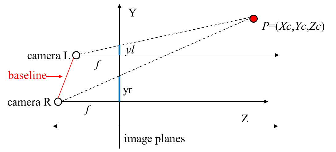
As shown in Figure 8, in a rectified stereo depth camera configuration with row-aligned image planes and negligible lens distortion, the projections of the same 3-D scene point onto the left and right images exhibit identical vertical coordinates, i.e., $$yl =yr$$. Consequently, depth estimation relies exclusively on the horizontal; the vertical coordinate does not participate in the triangulation process, and therefore, no additional constraints along the Y-axis are required in the stereo depth model.

Once the depth 𝑍 is estimated, the corresponding 3D spatial coordinates $$\left({X}_{c},{Y}_{c},{Z}_{c}\right)$$ can be reconstructed by applying the inverse projection from Equation (2). As illustrated in Figure 9 the principle of inverse projection describes the transformation from two-dimensional image coordinates to three-dimensional spatial coordinates. The camera center $$O$$ is defined as the origin of the camera coordinate system, with the Z-axis aligned with the optical axis, representing the depth direction. The focal length 𝑓 denotes the perpendicular distance between the camera center $$O$$ and the image plane, serving as the projection scaling factor in the pinhole model. In this framework, a spatial point $$\left({X}_{c},{Y}_{c},{Z}_{c}\right)$$ is projected onto the image plane at pixel coordinates $$\left(u, v\right)$$.

As illustrated in Figure 9, the principle of inverse projection highlights the transformation from two-dimensional pixel coordinates $$\left(u, v\right)$$ to three-dimensional spatial coordinates. The camera center $$O$$ is defined as the origin of the camera coordinate system, with the Z-axis aligned with the optical axis, representing the depth direction. The focal length $$f$$ denotes the perpendicular distance between the camera center $$O$$ and the image plane, serving as the projection scaling factor in the pinhole camera model. In this model, a spatial point $$\left({X}_{c},{Y}_{c},{Z}_{c}\right)$$ is projected onto the image plane as pixel coordinates $$\left(u, v\right)$$. The forward projection can be expressed as:

Conversely, when the depth value $${Z}_{c}$$ is known, the 3D spatial coordinates can be recovered through the inverse projection as:

This equation establishes a direct mapping from the image coordinates $$\left(x, y\right)$$ to the corresponding spatial coordinates $$\left({X}_{c},{Y}_{c},{Z}_{c}\right)$$. Here, 𝑥 and y denote the horizontal and vertical image coordinates in physical units (e.g., millimeters or meters), while $$\left(u, v\right)$$ represent the pixel coordinates on the image plane. The parameters $${f}_{x}$$ and $${f}_{y}$$ are the focal lengths of the camera, expressed in pixels, $${c}_{x}$$ and $${c}_{y}$$ represent the principal point coordinates, which define the optical center of the image. The variable $${Z}_{c}$$ corresponds to the depth value of the point along the optical axis, which determines the scale of the back-projection from the image plane to the spatial domain. This inverse projection process provides the theoretical foundation for vision-based 3D reconstruction, object localization, and motion tracking, and it plays a crucial role in binocular stereo vision, RGB-D imaging systems, and simultaneous localization and mapping (SLAM) frameworks.

To validate the effectiveness of the proposed flexible membrane floating body tracking system based on the YOLOv8 algorithm and a stereo depth camera, synchronous data acquisition experiments were conducted. The objectives of the experiment were twofold: first, to evaluate whether the system can efficiently and accurately track the target; and second, to verify whether the obtained displacement data can be reliably used for analyzing the membrane’s motion response.

As shown in Figure 10, the experimental setup was carefully designed to ensure measurement accuracy and repeatability. A gyroscope was installed at the front section of the structural model as the primary reference sensor. To facilitate stereo vision tracking, a red calibration target was firmly attached to the exposed surface of the gyroscope. To minimize potential optical interference and reflection artifacts, the area surrounding the calibration target was covered with black waterproof tape, thereby reducing background noise and enhancing the accuracy of image-based measurements.

For the purpose of validation, three representative wave conditions were selected, corresponding to incident wave heights of 3 m, 4 m, and 5 m in prototype scale. Different wave conditions were generated by adjusting the wave maker parameters, with input amplitudes set to 0.06 m, 0.08 m, and 0.1 m, while maintaining a constant wave period of 9.9 s to ensure comparability across tests. Under these test conditions, the gyroscope continuously recorded high-resolution acceleration and tilt signals to directly measure the dynamic response of the model. Simultaneously, the stereo camera system captured the 3D displacement of the red calibration target, enabling precise tracking of the model’s spatial motion. The combination of these two measurement systems provides a reliable basis for comparative analysis and lays the foundation for validating the stereo vision-based measurement approach. As shown in Figure 11, Figure 12, Figure 13, Figure 14, Figure 15 and Figure 16, the blue curves represent measurements from the stereo depth camera, while the red curves correspond to data collected by the gyroscope.

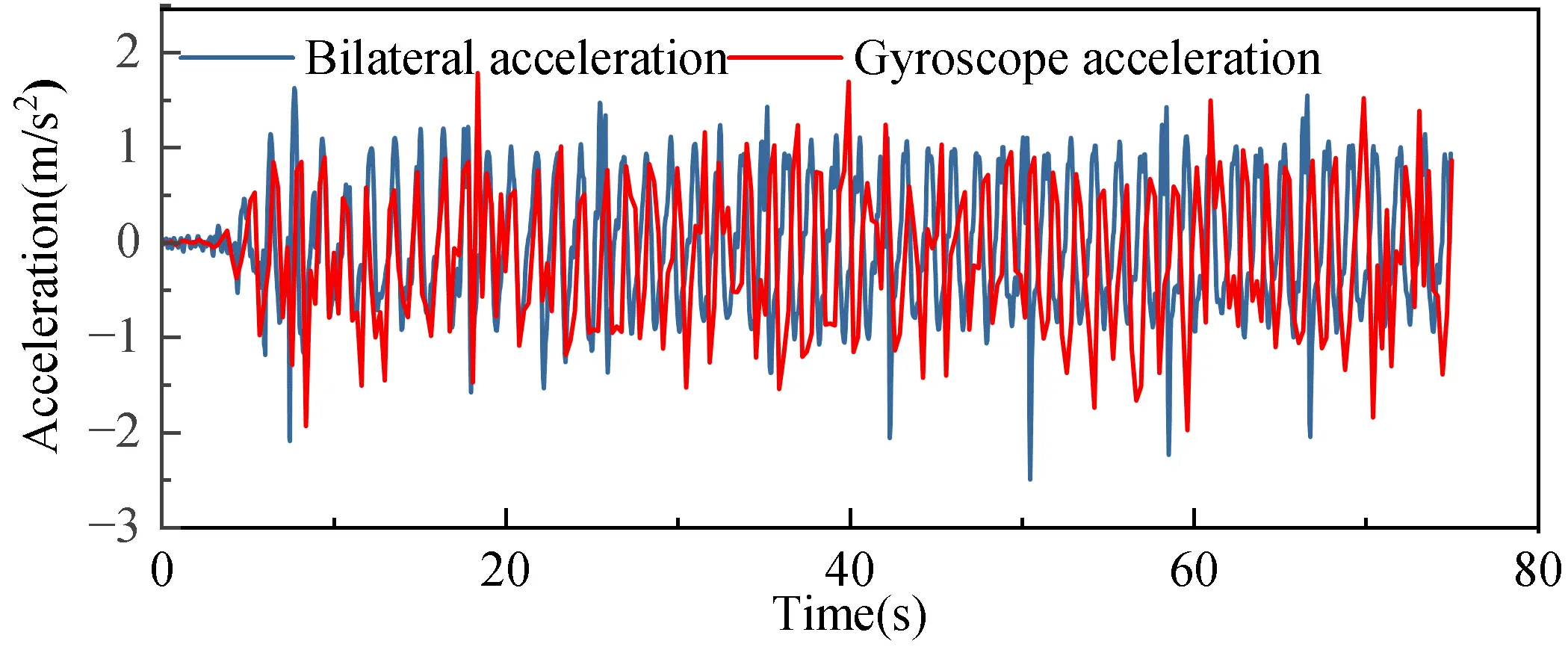
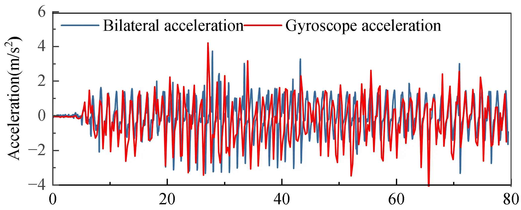
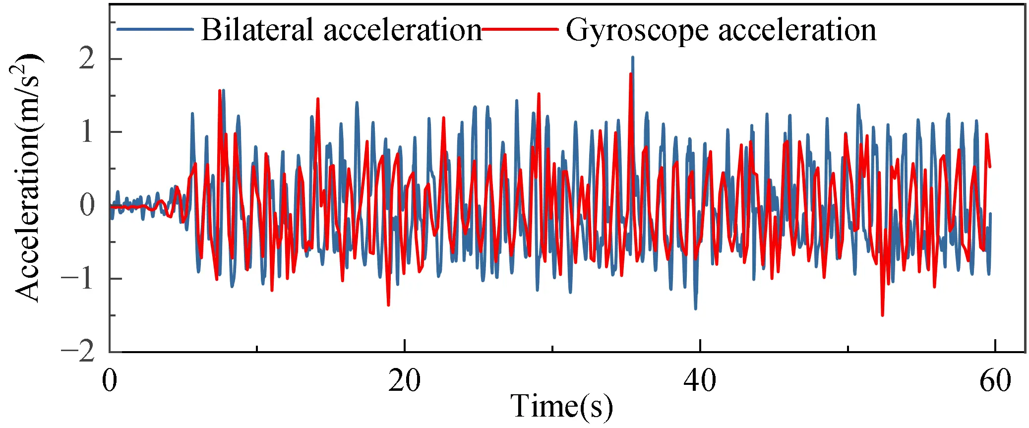
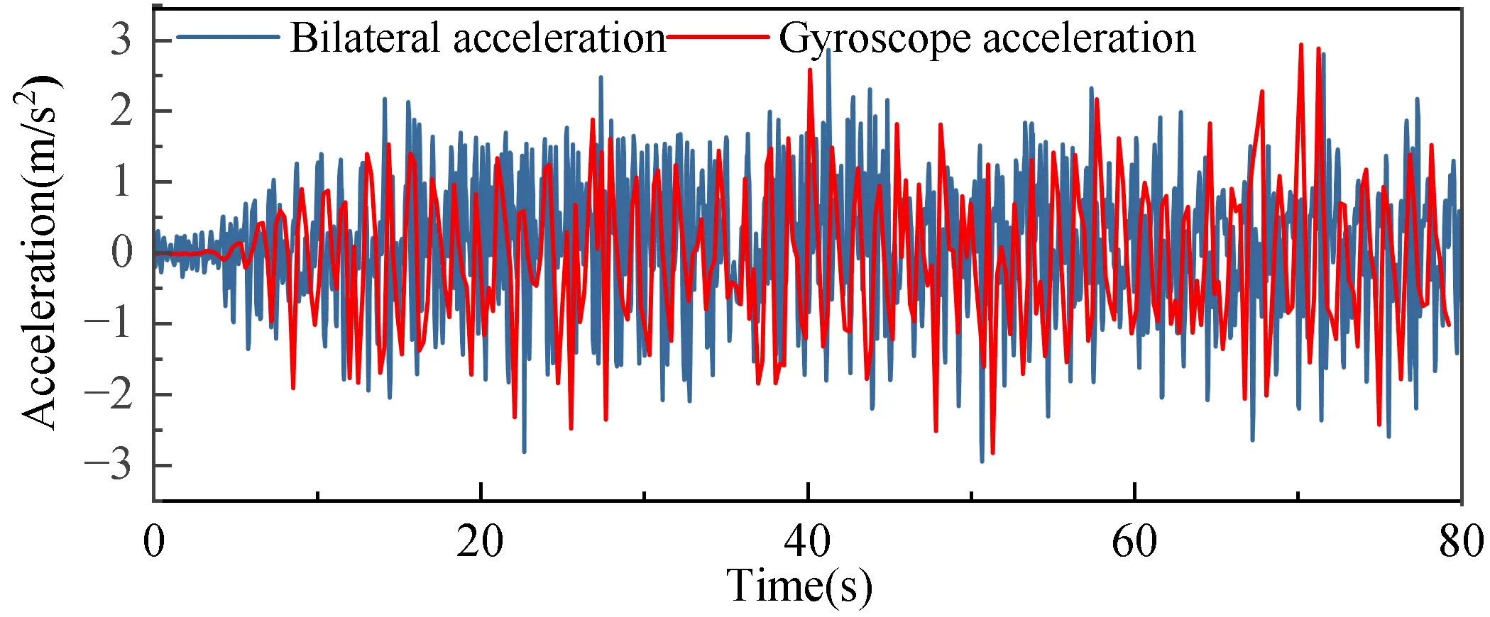
The position and timestamp data collected by the stereo camera were first post-processed to derive acceleration, which was then compared with the acceleration data obtained from the gyroscope. The comparison was conducted along the x- and z-directions, as illustrated in Figure 11, Figure 12, Figure 13, Figure 14, Figure 15 and Figure 16. The results indicate that the acceleration time histories measured by the gyroscope exhibit high consistency with those derived from the stereo camera data in both directions. To quantitatively assess this consistency, Figure 17 presents the mean squared error (MSE) corresponding to the comparisons shown in Figure 11, Figure 12, Figure 13, Figure 14, Figure 15 and Figure 16, providing a numerical measure of the deviation between the two measurement methods.

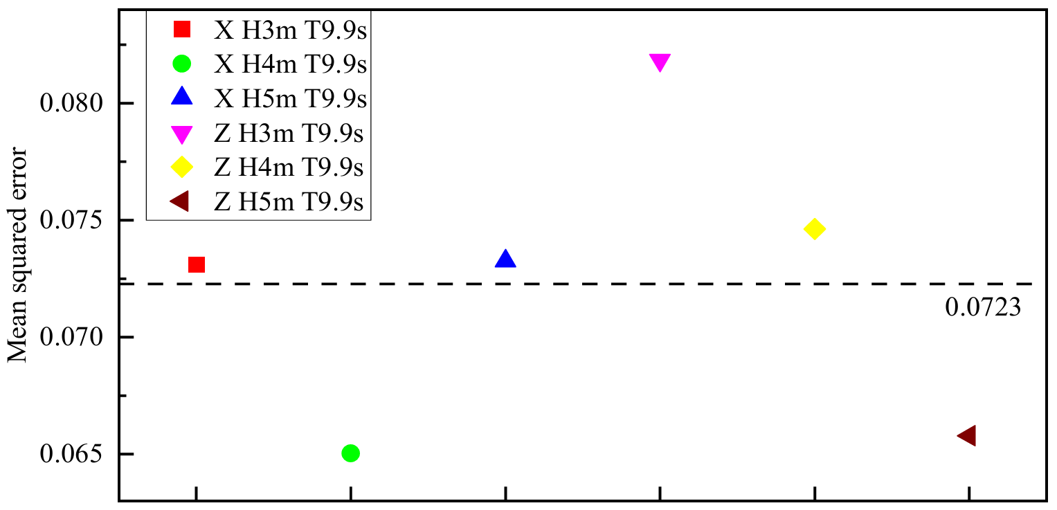
As shown in Figure 17, the mean squared error (MSE) values range from 0.065 to 0.082, with an overall average of 0.0723. These results indicate that the numerical deviations between the stereo depth camera and the gyroscope are within an acceptable range, thereby validating the reliability and accuracy of the stereo camera as an alternative measurement method. The observed minor discrepancies may primarily arise from limitations in time synchronization between the two measurement systems, potential noise introduced during the stereo camera image recognition process, and inherent sensor drift of the gyroscope. In addition, slight differences in the spatial positioning of the measurement reference points, as well as variations in the gyroscope’s installation height relative to the reference plane, may also contribute to these deviations.

As shown in Figure 4, the measurement points were arranged on the structure. Figure 18 and Figure 19 present the acceleration data along the x and z directions for different wave periods (6 s, 8 s, 9.9 s, and 12 s) under the same wave height condition. Data points with different colors and marker shapes represent different measurement locations, and their distributions are shown in Figure 18.

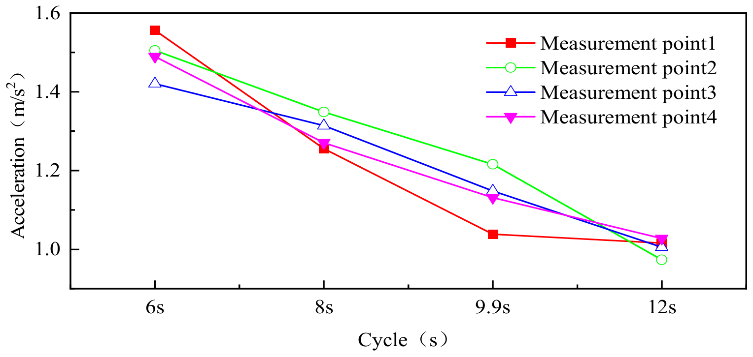
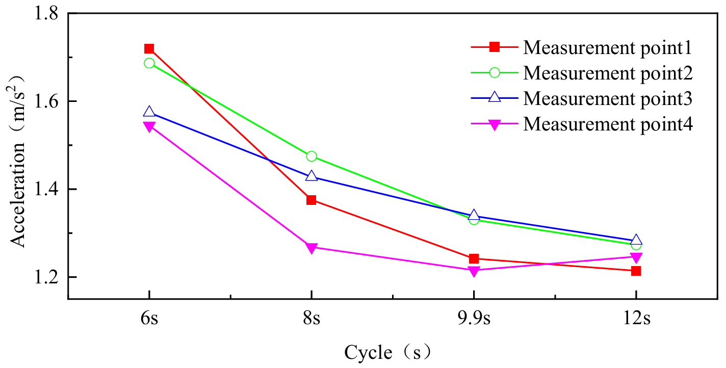
The results shown in Figure 18 and Figure 19 indicate that as the wave period increases, the rate at which the structure’s acceleration decreases gradually slows down. Under a constant wave height, as the wave period increases from 6 s to 12 s, the accelerations in both the horizontal (x) and vertical (z) directions exhibit an overall decreasing trend; however, the rate of decrease is not uniform across different intervals. Regarding the horizontal (x) acceleration: when the wave period increases from 6 s to 8 s, the average acceleration decreases by approximately 14.7%; from 8 s to 9.9 s, it decreases by 12.6%; and from 9.9 s to 12 s, the reduction slows further to only 11.7%. The vertical (z) acceleration exhibits a similar but more pronounced trend: a 15.3% decrease from 6–8 s, 7.55% from 8–9.9 s, and a minimal reduction of 2.3% from 9.9–12 s. These results indicate that as the wave period lengthens, the rate of acceleration attenuation gradually diminishes, reflecting a “diminishing marginal effect”.

From a physical perspective, this phenomenon can be explained by the dynamic interaction between wave excitation and structural inertia. As the wave period increases, the corresponding wave frequency decreases, which directly reduces the inertial forces acting on the structure, thereby lowering the acceleration amplitude. However, as the wave period extends further, the energy density of the wave excitation tends to stabilize, resulting in smaller increments of energy input per unit time. This causes the rate of acceleration decay to gradually slow down, ultimately leading to a nonlinear weakening of the structural response.

As shown in Figure 20 and Figure 21, the acceleration responses in the x and z directions are presented for different wave heights (3 m, 4 m, 5 m, and 6 m) under a constant wave period condition. Different colors and marker shapes in the figures represent different measurement points, with their spatial distribution shown in Figure 4.

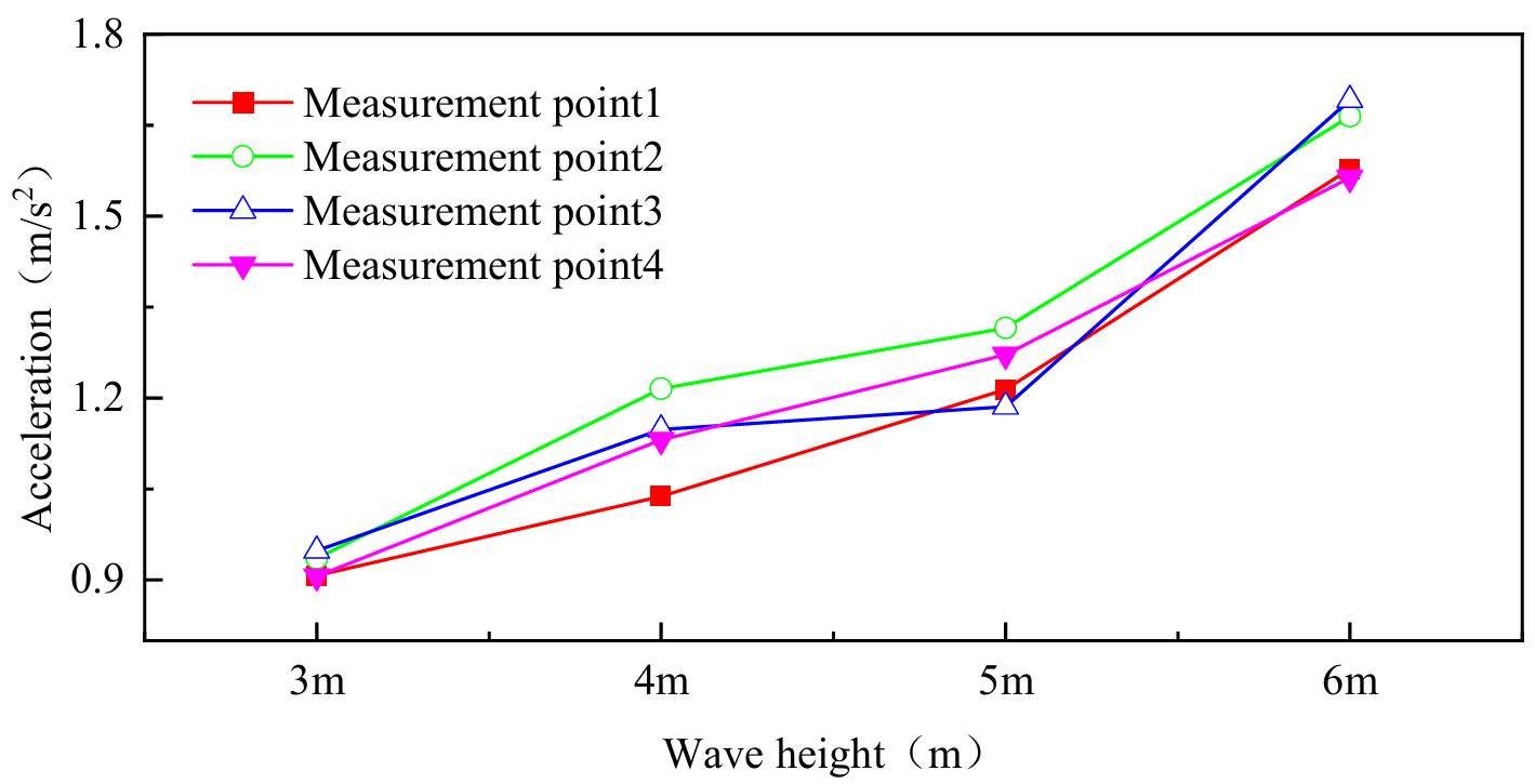
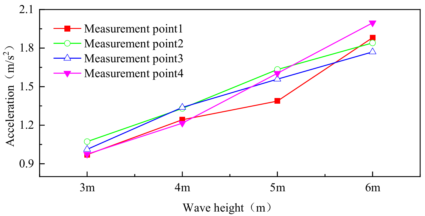
As shown in Figure 20 and Figure 21, under a constant wave period, the acceleration responses of the structure in all directions increase significantly with wave height. This trend is particularly pronounced within the representative wave period range of 6 s to 12 s. Taking the x-direction as an example, when the wave height increases from 3 m to 4 m, the average acceleration rises by approximately 21.22%; from 4 m to 5 m, it further increases by 10%; and from 5 m to 6 m, the increment significantly jumps to 30.4%. The z-direction acceleration exhibits a similar trend, but with slightly higher increments, reaching 27.3%, 20.5%, and 17.43% across the three respective intervals. These results indicate that, compared with wave period, wave height has a more direct and pronounced effect on structural acceleration. However, the increments across different wave height intervals are not uniform, exhibiting a clear stage-wise variation.

Conversely, under a constant wave height, structural acceleration generally decreases as the wave period increases. Statistical analysis indicates that for every 2 s increase in wave period, the average x-direction acceleration decreases by approximately 13%, while the average Z-direction acceleration decreases by about 8.3%. This attenuation pattern aligns with the expected reduction in inertial effects caused by lower wave frequencies, indicating that long-period waves, even at the same amplitude, exert weaker dynamic excitation on the structure.

Overall, under a constant wave period, the acceleration response exhibits an approximately linear relationship with wave height. Specifically, for every 1 m increase in wave height, the average x-direction acceleration increases by 20.54%, while the average z-direction acceleration rises by 21.74%. This nearly linear correlation indicates that wave height is the dominant factor determining the magnitude of structural acceleration, whereas wave period primarily influences the rate of response attenuation.

From the spatial distribution perspective, the acceleration magnitude at measurement point 1 is generally higher than at points 2, 3, and 4, although the differences are relatively small. This indicates that, at the scale of the present study, acceleration decay during wave propagation is not significant, implying a high degree of spatial uniformity in structural acceleration responses and strong spatial correlation of the wave-induced dynamic excitation across the structure.

From an engineering perspective, the key implication of the above findings is that increasing wave height significantly amplifies structural accelerations, thereby intensifying dynamic load effects and imposing stricter requirements on the safety and suitability of offshore structures. Although long-period waves gradually reduce structural accelerations, their attenuation effect is relatively limited, and the long-term impact should not be overlooked. Therefore, in the design and safety assessment of offshore structures, particular attention should be paid to structural responses under high wave heights, while also accounting for the cumulative effects of long-period waves.

This study proposes a non-contact motion monitoring and response analysis method for flexible floating photovoltaic (FPV) structures, based on binocular vision and deep learning techniques. By integrating a YOLOv8-based object detection algorithm with a binocular depth camera, a real-time monitoring system was developed that enables the extraction of three-dimensional coordinates and the identification of motion parameters. The system can accurately capture the dynamic behavior of flexible FPV structures under wave excitation without altering their hydrodynamic characteristics. The system performance was validated through physical model experiments, and the results were compared with gyroscope measurements, confirming the accuracy and stability of the proposed method. This study presents a novel experimental approach to investigate the dynamic responses of flexible FPV structures. The main conclusions are summarized as follows:

Although the proposed method performs well in experiments, several limitations remain. The experiments were conducted under controlled laboratory conditions, without fully accounting for environmental factors such as wind, illumination changes, and water surface reflections. Future research will focus on enhancing the robustness and stability of binocular depth cameras in complex wave environments. Algorithmic optimization and lightweight network architectures will be employed to improve depth computation efficiency and coordinate reconstruction accuracy. These efforts aim to enhance the system’s reliability in real ocean environments, providing technical support for the safe and long-term operation of FPV systems.

During the preparation of this work, the authors used ChatGPT in order to improve readability and language. After using this tool/service, the authors reviewed and edited the content as needed and take full responsibility for the content of the publication.

Conceptualization, S.Y.; Methodology, S.Y. and X.Y.; Software, S.Y.; Validation, S.Y. and L.Y.; Formal Analysis, S.Y.; Investigation, S.Y.; Resources, J.L., X.Y., Y.Y. and C.L.; Data Curation, S.Y.; Writing—Original Draft Preparation, S.Y.; Writing—Review & Editing, X.Y.; Visualization, S.Y.; Supervision, J.L., Y.Y. and C.L.; Project Administration, J.L., X.Y. and Y.Y.; Funding Acquisition, J.L., X.Y. and Y.Y.

Not applicable. This study did not involve humans or animals.

Not applicable. This study did not involve human participants.

The data presented in this study are available on reasonable request from the corresponding author. The data are not publicly available due to their large size and subsequent ongoing research.

This work was supported by the National Key R&D Program of China under Grant Number 2022YFB4200701, and National Natural Science Foundation of China under Grant Number 52571308, and Natural Science Foundation of Tianjin under Grant Number 24JCYBJC00870.

The authors declare that they have no known competing financial interests or personal relationships that could have appeared to influence the work reported in this paper.