Performance Evaluation of Machine Learning Algorithms for Predicting Organic Photovoltaic Efficiency

Performance Evaluation of Machine Learning Algorithms for Predicting Organic Photovoltaic Efficiency
Received: 26 July 2025 Revised: 02 September 2025 Accepted: 21 October 2025 Published: 31 October 2025

© 2025 The authors. This is an open access article under the Creative Commons Attribution 4.0 International License (https://creativecommons.org/licenses/by/4.0/).
1. Introduction
OSCs (Organic solar cells) are a promising solar technology. They have unique benefits, such as mechanical flexibility, low-temperature processing, and compatibility with lightweight, semi-transparent devices. Unlike traditional silicon-based solar cells, OSCs use organic semiconductor materials. These materials allow for adjustable optoelectronic properties through molecular design. However, efficiency and stability are still major challenges that prevent the widespread use of OSCs. The PCE of OSCs is affected by various material and device factors. These include the highest occupied molecular orbital (HOMO) and lowest unoccupied molecular orbital (LUMO) energy levels, optical band gap, charge carrier mobility, and the molecular structure of both donor and acceptor materials. Historically, improving these factors has involved slow and expensive experimental tests. To speed up the discovery and development of effective OSC materials, researchers are now using data-driven methods, especially ML techniques. Several recent studies have explored how ML algorithms can predict PCE in OSCs. For example, Lopez et al. [1] used random forest and kernel ridge regression models along with molecular descriptors to predict PCE, showing the promise of ensemble learning in this field. Sun et al. [2] applied deep neural networks to learn hierarchical features from molecular fingerprints, resulting in better prediction accuracy. At the same time, Zeng et al. [3] used support vector regression (SVR) and Gaussian process regression (GPR) for effective PCE estimation. These studies demonstrate how ML can speed up material screening but also point out some challenges, such as limited interpretability, a lack of model diagnostics, and a narrow comparative scope among algorithms. Most existing works focus either on traditional ML models or on deep learning alone, without comparing different model types within a single framework. Feature importance and model interpretability, which are essential for helping experimentalists in material design, are often ignored. Few studies rigorously evaluate models with cross-validation, hyperparameter tuning, and diagnostic visualizations such as learning curves and SHAP (SHapley Additive exPlanations) analysis. Zhao et al. [4] used graph neural networks to capture structure-property relationships in non-fullerene acceptors. They achieved high accuracy and provided insights into molecular design. Similarly, Li et al. [5] demonstrated how transfer learning can generalize efficiency predictions across multiple OSC datasets. This approach reduces the need for large training sets. Another study by Wang et al. [6] applied interpretable ML models to extract the chemical descriptors most relevant to device performance. This improved the transparency of efficiency predictions. Together, these studies show that ML not only boosts prediction accuracy but also speeds up materials discovery by highlighting key descriptors. The novelty of this study is in offering a thorough comparison of traditional regression models and machine learning algorithms for predicting PCE. We apply multiple linear regression (MLR), partial least squares (PLS), random forest (RF), XGBoost (XGB), and a multilayer perceptron (MLP) to a selected dataset of donor and acceptor materials. Our process includes cleaning diverse features, tuning hyperparameters with randomized search, and evaluating performance using R2, RMSE, and MAE metrics. Our framework is more than just a focus on predictive accuracy. We offer clear model interpretation using permutation feature importance and SHAP summary plots. We investigate how the models learn through learning curves and convergence plots, and we evaluate model robustness with partial dependence plots (PDP), individual conditional expectation (ICE) plots, and calibration curves. This approach allows for accurate predictions and a deeper understanding of the structure-property relationships in OSC materials. Our findings show that the tuned XGBoost model performs best, achieving an R2 of 0.980 and an RMSE of 0.564 on the test set. The most important features we found include HOMO and LUMO levels, electrochemical bandgap, and electronic mobility. Including SHAP analysis clarifies complex models, making the predictions clearer and easier to validate through experiments.
In summary, this work offers a strong, clear, and reproducible ML pipeline for OSC PCE prediction. It combines traditional regression with modern ML methods. Our results can guide future studies on efficient screening of organic photovoltaic materials. They also provide a basis for incorporating ML into experimental workflows. This study helps speed up discovery in organic photovoltaics through machine intelligence.
2. Materials and Methods
This section describes the method used to predict the PCE of OSC materials with traditional and modern ML models. The method includes data processing, model training and evaluation, hyperparameter tuning, and result analysis.
2.1. Dataset Description and Preprocessing
Dataset Description
The dataset includes donor and acceptor molecules with validated PCE values and various chemical and electronic descriptors. The raw data derived from published sources and practical lab tests and was stored in an Excel file. This dataset partly stems from literature found in peer-reviewed journals that focus on organic photovoltaic materials and PCE screening standards. Each entry contains both numerical features, such as the HOMO-LUMO gap, electron affinity, ionization potential, and mobility values, and categorical features, including molecular structures and material types.
2.2. Data Preprocessing
2.2.1. Scientific Notation Handling
Some features, such as electronic mobility, were expressed using superscript scientific notation (e.g., 2.1 × 10⁻⁴). These were programmatically converted into floating-point numbers using Python’s “re” and “float” handling.
2.2.2. Feature Engineering
Numerical features like HOMO, LUMO, band gap, electron affinity, ionization potential, and charge mobility were standardized using the StandardScaler to have a zero mean and a variance of one. Categorical features, such as donor/acceptor material type, were transformed using one-hot encoding, which created binary variables for each category. These preprocessing steps were put together in a ColumnTransformer pipeline, ensuring consistency in both the training and test sets.
2.3. Model Development
This section describes the ML models used for PCE prediction. These models were selected for their effectiveness in regression tasks and their previous success in related materials research. Traditional models like MLR and PLS provide clear insights and serve as baselines. RF and XGBoost are popular because they manage complex nonlinear relationships and feature interactions well. Deep learning models like MLP have shown great performance in capturing intricate patterns in molecular and electronic data, which supports their inclusion in this study.
2.3.1. Test-Train Split
The dataset was split into training and testing sets using an 80:20 ratio. The “train_test_split” function from “sklearn.model_selection” was used with a random seed of 42 for reproducibility.
2.3.2. Traditional ML Models
The following traditional models were implemented based on their historical relevance and interpretability in regression modeling:
-
-
MLR is a basic statistical model that estimates the linear relationship between input features and a continuous target. Its simplicity makes it easy to understand and serves as a standard for more complex models. MLR is widely used in predicting photovoltaic performance because it is straightforward to analyze [7].
-
-
PLS is particularly useful for high-dimensional, multicollinear data. PLS regression projects predictors into a smaller latent space and keeps the most important covariance with the response variable. In this study, we focused on two components to reduce dimensional noise and maintain key predictive signals [8].
-
-
RF is a non-parametric ensemble method that combines predictions from several decision trees. Its strength against overfitting and its ability to model complex nonlinear interactions make it suitable for datasets with different types of features. RF has shown effectiveness in earlier materials informatics tasks, including predicting the performance of organic solar cells [9,10].
2.3.3. Advanced ML Models
To capture complex nonlinear relationships in OSC material data, we also used advanced models, including XGBoost and a custom-designed MLP neural network. We chose these models because they have shown better performance in different regression and tabular prediction tasks.
-
-
XGBoost: XGBoost is an improved gradient boosting framework that builds decision trees one after another. It uses regularization to prevent overfitting. The framework supports parallel computation and can handle missing values, making it very effective for problems involving structured data. We used both the default version and the one with adjusted hyperparameters. Previous studies in materials science have effectively used XGBoost because of its scalability and accuracy [11].
-
-
Hyperparameter Tuning for XGBoost: We used a 5-fold cross-validated “RandomizedSearchCV” to improve generalization. We focused on parameters such as tree depth, learning rate, and subsampling ratio. This approach significantly improved performance by reducing the RMSE on unseen data.
-
-
MLP: A feed forward neural network that can learn any nonlinear relationships. The built architecture has two hidden layers with 64 and 32 neurons, respectively, using ReLU activation and early stopping to avoid overfitting. MLPs are good at identifying subtle, complex patterns in both numeric and categorical data. They have shown potential in predicting photovoltaic efficiencies [12]. Training used the Adam optimizer and MSE as the loss measure.
The choice to include XGBoost and MLP came from the need to capture complex, nonlinear relationships in the OSC dataset. Linear models may struggle to represent these dependencies. These models have shown strong predictive performance in regression tests related to chemical informatics, material discovery, and energy systems [13].
2.3.4. Regression Metrics
To evaluate model performance comprehensively, we utilized the following standard regression metrics:
-
-
Mean Squared Error (MSE): MSE measures the average of the squares of the errors, the average squared difference between the predicted and actual values. It penalizes larger errors more heavily and is defined as:
| ```latexMSE=\frac{1}{n}\sum_{i=1}^{n}(y_{i}-\hat{y}_{i})^{2}``` |
MSE is widely used in regression tasks due to its mathematical convenience and sensitivity to large errors [14].
-
-
Root Mean Squared Error (RMSE): RMSE is the square root of the MSE and provides a metric in the same unit as the target variable. It is often used in energy-related prediction studies due to its interpretability [15].
| ```latexRMSE=\sqrt{\frac{1}{n}\sum_{i=1}^n(y_i-\widehat{y}_i)^2}``` |
-
-
Mean Absolute Error (MAE): MAE represents the average magnitude of errors in a set of predictions, without considering their direction. It is less sensitive to outliers than RMSE and offers a robust performance evaluation [16].
| ```latexMAE=\frac{1}{n}\sum_{i=1}^n|y_i-\hat{y}_i|``` |
-
-
Coefficient of Determination (R2): R2 measures how much of the variation in the dependent variable can be predicted from the independent variables. An R2 of 1 shows perfect prediction, while 0 indicates no predictive ability. It offers a standardized way to assess how well the model fits [17].
| ```latexR^2=1-\frac{\sum_{i=1}^n(y_i-\hat{y}_i)^2}{\sum_{i=1}^n(y_i-\bar{y}_i)^2}``` |
These metrics collectively provide insights into both the accuracy and robustness of each model and are commonly used in ML and materials informatics literature.
2.4. Cross-Validation and Hyperparameter Tuning
To ensure fair evaluation and reduce overfitting, we used a standard procedure for all machine learning models. Each model was tested with 5-fold cross-validation (CV), where the dataset was randomly split into five equal subsets. In each round, four subsets were used for training and one for validation. This process was repeated five times, so every sample was used as a validation point once. We averaged the final performance metrics over the folds, giving a balanced estimate of each model’s bias, variance trade-off, and ability to generalize. All models used the same preprocessing pipeline, feature set, and data partitions to ensure strict comparability. We fixed random seeds, metric definitions, and scaling parameters across experiments. For model optimization, we used RandomizedSearchCV to efficiently explore hyperparameter combinations within predefined ranges. We mainly applied hyperparameter tuning to XGB and MLP because their performance is very sensitive to parameter choices and regularization strength. We included baseline models for interpretability and comparison; early experiments showed that further tuning led to only small improvements over their default settings. The optimized parameters for the tuned models are summarized in Table 1.
Table 1. Summary of optimized parameters for the tuned models.
|
Model |
Hyperparameter |
Best Value |
|---|---|---|
|
XGBoost |
max_depth |
5 |
|
learning_rate |
0.05 |
|
|
subsample |
0.8 |
|
|
n_estimators |
200 |
|
|
MLP |
hidden_layer_sizes |
(64, 32) |
|
activation |
ReLU |
|
|
alpha (L2 regularizer) |
0.001 |
|
|
learning_rate_init |
0.001 |
This unified experimental protocol ensures that each model was trained, validated, and compared under the same conditions, allowing for reproducibility and a clear evaluation of each algorithm’s predictive ability.
3. Results
In this section, we compare how well different machine learning models can predict the efficiency of organic solar cells. To evaluate their performance, we used common measures like how close the predictions were to the actual values (RMSE and MAE) and how well the models explained the variation in the data (R2). The findings clearly show that more complex models, like XGBoost and deep neural networks, performed better than simpler models such as linear regression.
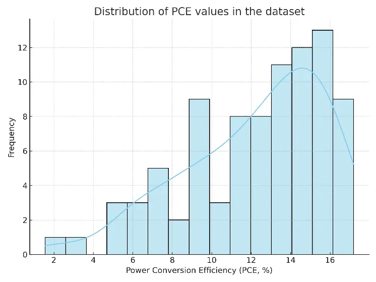
Before comparing model performance, we looked at the distribution of PCE values in the dataset (Figure 1). The values are not evenly spread out. Most OSCs fall into the mid-efficiency range, typically between 8% and 15%. However, only a few samples go above 18%. This uneven distribution shows the current state of OSC experiments, where high-efficiency devices are still uncommon. This imbalance has two effects. First, models might be biased toward predicting mid-range PCEs, which can lead to underestimating outliers. Second, having fewer high-efficiency samples makes it more difficult for models to generalize in that area.
Model Performance Comparison
Table 2 summarizes how each model performed, and we provide further visual explanations to understand why these models worked better.
Table 2. Performance metrics of machine learning models.
|
Model |
RMSE |
MAE |
R2 |
|---|---|---|---|
|
MLR |
0.964 |
0.763 |
0.943 |
|
PLS (n = 2) |
2.052 |
1.582 |
0.742 |
|
RF |
0.889 |
0.686 |
0.951 |
|
XGB (default) |
1.086 |
0.713 |
0.928 |
|
XGB (tuned) |
0.564 |
0.446 |
0.980 |
The tuned XGBoost model outperformed all others, achieving the lowest RMSE of 0.564 and the highest R2 of 0.980. This demonstrates strong generalization and predictive power. Random Forest also performed well, followed by the default XGB and MLR. The PLS model showed limited effectiveness because of multicollinearity and linear assumptions. Although RF showed competitive performance, we chose XGB for detailed optimization. Boosting frameworks fix errors from earlier models step by step and include regularization to prevent overfitting. After tuning, XGB outperformed RF in both RMSE and R2, proving its better generalization ability for this dataset.
To see how model performance changes with more training data, we created a learning curve for the tuned XGBoost model (Figure 2). The curve displays the RMSE for both the training and validation sets across various training set sizes. Training RMSE stays consistently low, indicating that the model fits the training data exceptionally well with very little error. Validation RMSE decreases steadily as we add more training data, eventually leveling off around a set size of 45 to 55. This shows that the model improves with more data and performs better with larger training sets. The widening gap between training and validation RMSE in the early stages suggests some overfitting, which diminishes as we introduce more data. Overall, the model shows good generalization with little variation at larger dataset sizes.
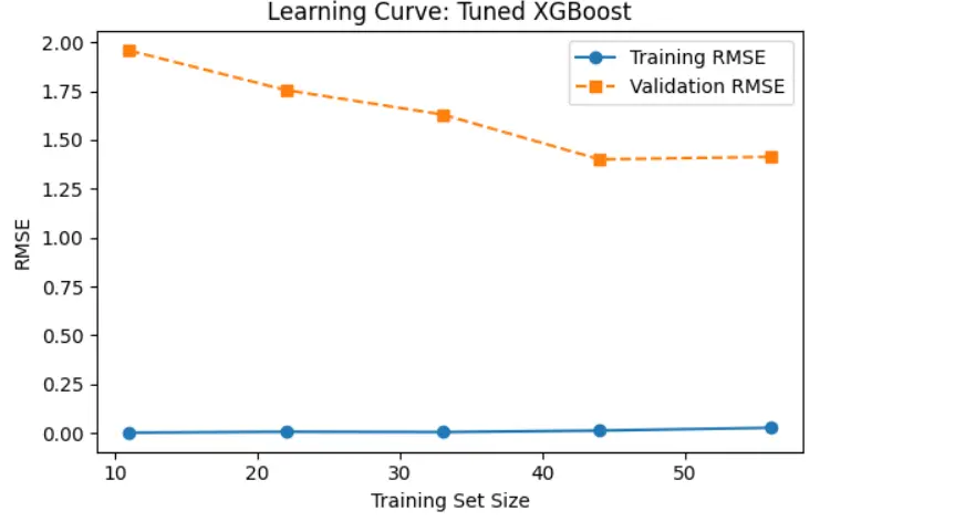
Figure 2. The learning curve shows that increasing the training set size reduces validation RMSE and narrows the generalization gap, improving model performance.
The histogram is in Figure 3 shows the distribution of residuals (Predicted—True values) for the regression model’s predictions. The residuals range from about −1.2 to +0.7, reflecting the spread of prediction errors. The highest frequency bins are around 0 and −0.8, indicating that most predictions are quite accurate, with errors close to zero. There is a noticeable concentration of residuals between −1.0 and +0.3, which shows that the model works well on most test samples. The shape of the histogram is mostly symmetric but slightly skewed to the negative side. This indicates the model tends to overpredict (meaning the predicted value is often higher than the actual value) more than it underpredicts. There are no extreme outliers, and the spread of residuals is narrow. This suggests a low variance in prediction errors. Overall, this pattern implies a good fit between the predicted and actual values, showing no strong bias and generally consistent performance.
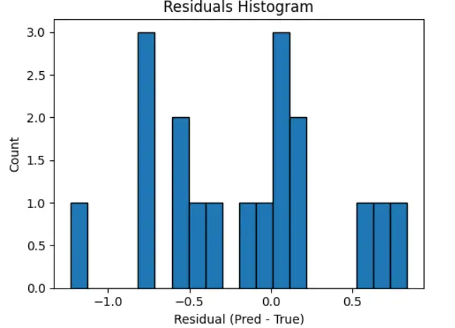
Figure 3. Residuals histogram for the tuned XGBoost model. The residuals (difference between predicted and true PCE values) are centered around zero, indicating minimal prediction bias. The distribution is moderately symmetric, with most residuals falling within a narrow range, suggesting consistent model performance and low variance in prediction errors.
The calibration curve shown in Figure 4 compares the average predicted PCE to the average true PCE across several bins of prediction intervals. The blue line with markers represents the relationship derived from the model’s outputs, while the red diagonal line indicates perfect calibration, where predicted values match the true outcomes exactly. We see that the blue curve closely follows the ideal diagonal line, especially in the mid-to-high prediction range (around 10 to 17). This suggests that the model is well-calibrated in those areas. When the model predicts a certain PCE value, the actual observed value is very close on average. In the lower prediction range (mean predicted PCE between 6 and 9), there is a slight dip below the ideal line. This shows a minor underestimation of PCE by the model in that region. However, this difference is not significant and becomes negligible as the predicted values increase. The steady nature of the calibration curve across the entire prediction range shows that the model predicts reliable values and maintains trust in its uncertainty estimates. This builds confidence in the model’s predictions for real-life applications like materials discovery or device design. To further explore the areas in the feature space where the prediction model shows higher or lower error, we created a 2D error heatmap using two important material descriptors: Acceptor Band Gap and Jsc. In this plot, the x-axis shows binned values of the Acceptor Band Gap, while the y-axis shows binned values of Jsc. The color intensity in each bin reflects the mean absolute residual, which is the average absolute difference between the predicted and actual PCE values for data samples in that bin. A brighter color, like yellow, indicates a higher prediction error, while darker shades, such as deep purple, represent areas with low residuals and higher prediction accuracy.
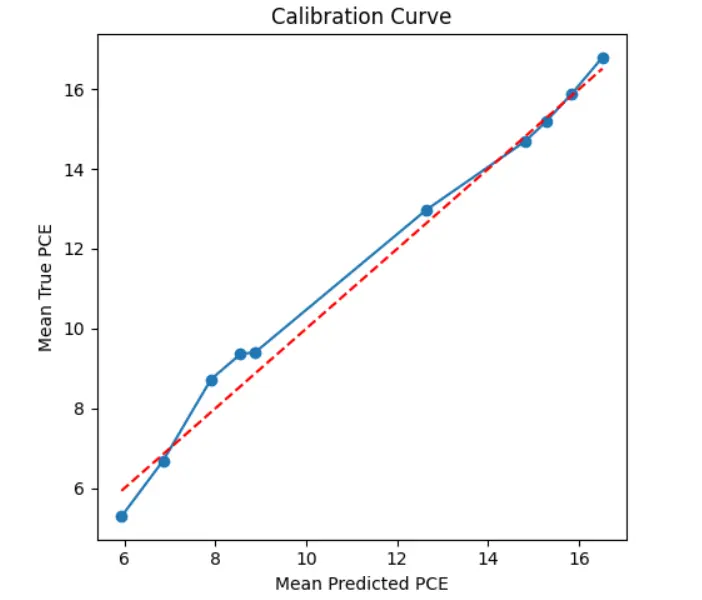
Figure 4. Calibration curve comparing the mean predicted PCE to the mean true PCE across prediction intervals. The blue curve represents the actual calibration of the model, while the red dashed diagonal line indicates perfect calibration. The close alignment of the blue curve to the diagonal suggests that the model is well-calibrated.
Jsc and acceptor band gap were chosen as axes for the error heatmap because both parameters have a strong impact on photocurrent generation and exciton separation in OSCs. This choice, while exploratory, shows how prediction error changes across ranges of material properties that are directly related to device performance. Areas with very low Jsc values and highly negative acceptor band gaps have the largest prediction errors. This pattern may be due to either a lack of data in these edge areas or the model’s inability to generalize well with less frequent material configurations. Conversely, moderate values of both descriptors are linked to much lower residuals, suggesting that the model understands these regions better, likely because of denser training data or more representative features. This heatmap offers important insights into the model’s uncertainty in predictions. It helps us pinpoint specific ranges of material properties where the model struggles. These visual tools are particularly helpful for guiding active learning strategies or data enhancement efforts to make the model more reliable in regions with fewer examples, as shown in Figure 5.
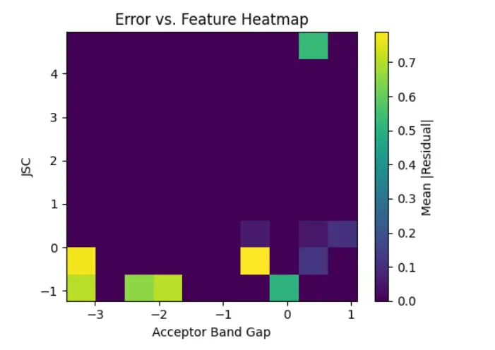
Figure 5. Heatmap illustrating the average absolute residuals between predicted and actual PCE values across binned values of Acceptor Band Gap and Jsc.
The plot in Figure 6 shows how changing the “max_depth” hyperparameter affects the CV RMSE for the XGBoost model. As the depth of the decision trees increases from 3 to 7, the mean RMSE rises slightly, indicating a small drop in model generalization. The error bars, which show the standard deviation across cross-validation folds, widen with greater depth. This suggests more variability in model performance. This trend means that while deeper trees can capture more complex patterns, they are also more likely to be overfit and less stable. The lower RMSE and tighter error bounds at max_depth = 3 indicate that it is the best setting for this dataset, providing a good balance between predictive performance and model stability.
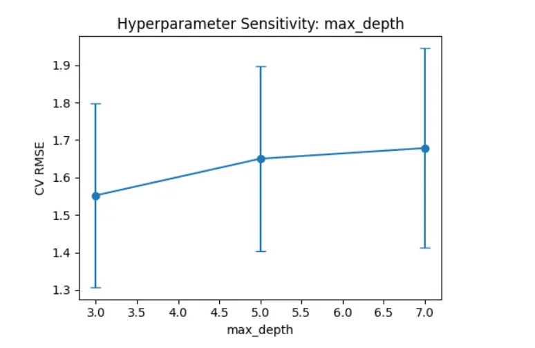
Figure 6. Cross-validated RMSE for different values of the max_depth hyperparameter in the XGBoost model. Error bars represent the standard deviation across cross-validation folds. The trend indicates increased RMSE and variability with deeper trees, suggesting overfitting at higher depths. The optimal performance is observed around max_depth = 3, balancing accuracy and generalization.
4. Discussion
The comparability of all models in this work resulted from a consistent experimental process that managed dataset splits, scaling, and evaluation metrics. This standardization allows for a direct and fair comparison of how algorithms perform. In addition to basic tuning, our contribution includes bringing together and explaining the performance of various ML approaches. These approaches include statistical regression, ensemble methods, and neural networks, all within one clear and reproducible framework. The results of this study show that ML techniques, especially gradient-boosted decision trees and deep neural networks, provide a notable edge in predicting OSC efficiencies. This importance lies not just in the numerical performance of models like tuned XGBoost, but in their ability to identify subtle, nonlinear relationships among material features; this is an area where traditional regression models often fall short. The shrinking gap between training and validation errors, along with consistently low residuals in most areas of the feature space, suggests that the best-performing models can generalize well. This means that, with enough representative data, machine learning can effectively replace or enhance traditional methods for estimating efficiency through simulations. Visual tools like calibration curves further demonstrate the strength and reliability of these models. The close match between predicted and actual values builds confidence in their predictions. This trust is essential for applications in material discovery and device optimization, especially when physical prototyping can be costly or time-consuming. These results also hint at a move towards automation in OSC screening processes. By reducing prediction errors and improving interpretability, the proposed pipeline shows promise in speeding up the material selection in organic photovoltaics. The better performance with more training data suggests that future advancements are likely as more extensive or varied datasets become accessible. However, while the models showed strong overall performance, understanding them remains challenging, particularly with neural networks. Tools that assess feature importance are helpful, but more work is necessary to convert these insights into specific design principles for the field. Additionally, areas within the feature space that display higher prediction errors indicate that targeted data enhancement could further improve results. The findings support the use of tuned machine learning models for precise PCE prediction and emphasize their potential to speed up research in next-generation solar technologies. These models not only boost predictive accuracy but also provide valuable insights that can inform future data gathering and material design strategies. To test robustness, we also performed preliminary evaluations using different train/test splits (70:30 and 75:25). The ranking of model performance remained consistent, with tuned XGB performing better than the others in every instance. This suggests that the results are stable across various data partitioning methods, although we will conduct more thorough sensitivity analyses in future. While hyperparameter optimization and validation are common practices, our innovation is in creating a reproducible benchmarking framework that links predictive accuracy with physical interpretability. We integrate diagnostic visualizations like SHAP, calibration, and error mapping. This provides insights into the relationships between features and efficiency, which can guide material design. This is an area that previous OSC machine learning studies rarely addressed.
5. Conclusions
This study shows how effective machine learning models are at predicting the PCE of OSCs. It uses a structured dataset that includes electronic and structural features of donor and acceptor materials. Among the models tested, the tuned XGBoost model had the highest prediction accuracy, with an RMSE of 0.564 and an R2 of 0.980. It clearly outperformed traditional models like Multiple Linear Regression and Partial Least Squares. The combination of preprocessing, feature transformation, and model-specific optimization improved performance across all models. Visualization tools such as residual plots, SHAP analysis, and learning curves gave better insights into model behavior, interpretability, and generalization. These tools showed that electronic descriptors like LUMO energy and electron mobility play a key role in predicting PCE. Overall, the study confirms that machine learning can effectively support experimental screening in the OSC field. The findings validate the use of advanced algorithms for regression tasks in material science. They also open possibilities for automated material selection, lower experimental costs, and faster discovery of high-efficiency organic photovoltaic materials. A limitation of this study is the relatively small dataset size. While the tuned XGB model performed well in cross-validation, future work should test its performance on larger, independent datasets of donor-acceptor pairs to further establish its reliability.
Author Contributions
Conceptualization, M.S.H. and S.Y.F.; Methodology, M.S.H.; Software, M.S.H.; Validation, M.S.H. and S.Y.F.; Formal Analysis, M.S.H.; Investigation, M.S.H.; Resources, M.S.H.; Data Curation, M.S.H.; Writing—Original Draft Preparation, M.S.H.; Writing—Review & Editing, M.S.H. and S.Y.F.; Visualization, M.S.H. and S.Y.F.; Supervision, S.Y.F.
Ethics Statement
Not applicable.
Informed Consent Statement
Not applicable.
Data Availability Statement
The dataset is currently in progress. We may be able to make it available after publication.
Funding
This research received no external funding.
Declaration of Competing Interest
The authors declare that they have no known competing financial interests or personal relationships that could have appeared to influence the work reported in this paper.
References
- Lopez SA, Sanchez-Lengeling B, de Goes Soares J, Aspuru-Guzik A. Design principles and top non-fullerene acceptor candidates for organic photovoltaics. Adv. Energy Mater. 2017, 1, 857–870. [Google Scholar]
- Sun W, Zheng Y, Yang K, Zhang Q, Shah AA, Wu Z, et al. Machine learning-assisted molecular design and efficiency prediction for high-performance organic photovoltaic materials. Sci. Adv. 2019, 5, eaay4275. [Google Scholar]
- Jiang Y, Yao C, Yang Y, Wang J. Machine learning approaches for predicting power conversion efficiency in organic solar cells: A comprehensive review. Solar RRL 2024, 8, 2400567. [Google Scholar]
- Zhao W, Zhang M, Yuan J, Li Y. Machine learning for organic solar cells. Adv. Mater. 2023, 35, 2300259. [Google Scholar]
- Mahmood A, Irfan A, Wang JL. Machine Learning for Organic Photovoltaic Polymers: A Minireview. Chin. J. Polym. Sci. 2022, 40, 870–876. doi:10.1007/s10118-022-2782-5. [Google Scholar]
- Siddiqui H, Usmani T. Interpretable AI and Machine Learning Classification for Identifying High-Efficiency Donor–Acceptor Pairs in Organic Solar Cells. ACS Omega 2024, 9, 34445–34455. doi:10.1021/acsomega.4c02157. [Google Scholar]
- Neves BJ, Braga RC, Melo-Filho CC, Moreira-Filho JT, Muratov EN, Andrade CH. QSAR-Based Virtual Screening: Advances and Applications in Drug Discovery. Front Pharmacol. 2018, 9, 1275. doi:10.3389/fphar.2018.01275. [Google Scholar]
- Geladi P, Kowalski BR. Partial least-squares regression: A tutorial. Anal. Chim. Acta 1986, 185, 1–17. [Google Scholar]
- Butler KT, Davies DW, Cartwright H, Isayev O, Walsh A. Machine learning for molecular and materials science. Nature 2018, 559, 547–555. [Google Scholar]
- Chen T, Guestrin C. XGBoost: A Scalable Tree Boosting System. In Proceedings of the 22nd ACM SIGKDD International Conference on Knowledge Discovery and Data Mining, San Francisco, CA, USA, 13–17 August 2016. [Google Scholar]
- Ahasan MR, Haque MS, Alam MGR. Supervised Learning Based Mobile Network Anomaly Detection from Key Performance Indicator (KPI) Data. In Proceedings of the 2022 IEEE Region 10 Symposium (TENSYMP), Mumbai, India, 1–3 July 2022; pp. 1–6. [Google Scholar]
- Yi C, Wu Y, Gao Y, Du Q. Tandem solar cells efficiency prediction and optimization via deep learning. Phys. Chem. Chem. Phys. 2021, 23, 2991–2998. doi:10.1039/D0CP05882C. [Google Scholar]
- Ward L, Agrawal A, Choudhary A, Wolverton C. A general-purpose machine learning framework for predicting properties of inorganic materials. NPJ Comput. Mater. 2016, 2, 1–7. [Google Scholar]
- Hyndman RJ, Koehler AB. Another look at measures of forecast accuracy. Int. J. Forecast. 2006, 22, 679–688. [Google Scholar]
- Willmott CJ, Matsuura K. Advantages of the mean absolute error (MAE) over the root mean square error (RMSE) in assessing average model performance. Clim. Res. 2005, 30, 79–82. [Google Scholar]
- Chai T, Draxler RR. Root mean square error (RMSE) or mean absolute error (MAE)? Arguments against avoiding RMSE in the literature. Geosci. Model Dev. 2014, 7, 1247–1250. [Google Scholar]
- Draper NR, Smith H. Applied Regression Analysis, 3rd ed.; Wiley-Interscience: Hoboken, NJ, USA, 1998. [Google Scholar]