1. Introduction
The information on land use and land cover is not just needed for today’s research era, but is an essential requirement in urban planning, regional planning, environmental impact assessment, and activities like natural and disaster risk management. Detecting changes over time is the best way to understand landscape transformation and its prediction. In the real-world land use is the way of using a parcel of land by living beings as per their requirement, while land cover means the physical condition of land resources present on the earth. They are both correlated with each other. Land use and land cover change assessment is truly required for a number of purposes, which are basically for the welfare of humans in the way of rapid and unstoppable growth in the population and because of extreme economic and industrial development. Changes in land use and land cover have multiple effects on the environment and human health in different ways, such as ecosystem loss, floods and droughts, depletion in groundwater, forest and land degradation, soil and water erosion and many more. Moreover, in public and private sectors, the demand for a deep study of land use and land cover is very high due to its vast utilization. Moreover, classification of land use land cover is the process of assigning different classes and categorizing them in metropolitan, agriculture, woodland, water, built-up, horticulture, grasslands and mountains,
etc. The Anderson classification is one of the standard classification systems for displaying the utilized land and its coverage [
1].
Satellite remotely sensed data comprises various LULC class information that must be extracted using advanced technologies. LULC changes are very dynamic in nature and need to be monitored on the basis of spatial and temporal changes. Traditional pixel-based approaches often face challenges in dealing with the inherent heterogeneity and complexity of remote sensing data. They fail to capture the spatial context and relationships among neighboring pixels, limiting their ability to extract high-level features and accurately classify land cover and land use (LULC) categories. In contrast, Object Based Image Analysis (OBIA)exploits the spatial and contextual information provided by image objects, resulting in improved classification accuracy and more robust analysis. A considerable body of literature has been dedicated to the development and application of OBIA techniques in remote sensing datasets. One of the key components of OBIA is image segmentation, which partitions an image into homogeneous and coherent objects. Various segmentation algorithms have been proposed, ranging from region-based methods such as mean-shift and graph cuts to edge-based methods like watershed and morphological techniques. These algorithms aim to delineate objects based on spectral, spatial, and textural characteristics, effectively capturing the inherent heterogeneity of remote sensing imagery. The technologies ranging from visual interpretation, semi–automatic OBIA to deep learning have been explored in extracting the image information.
The use of satellite images has increased exponentially from the past decades. Satellite data provides a single shot of a particular area at one point in time, giving the full view of any land cover. We can say that remote sensing provides us with the opportunity for continuous and rapid acquisition of information on land use and land cover. Land use and land cover are usually produced using classification techniques, but the accuracy and processing time are still challenging for our community. The Sentinel-2 (A&B) satellite data product is the latest generation earth observation mission specially designed for coastal and land applications. Due to its free access, it has a wide swath with high spatial resolution rage from 10–60 m. A wide range of studies have been conducted using Sentinel-2 satellite imageries
i.e., LULC mapping, crops and orchard classification, monitoring of forest stress, surface water mapping,
etc., but spatially in the study of LULC mapping, Sentinel-2 data has been tested and showed very high potential [
2,
3,
4,
5] However, because it is a recent type of satellite imagery, very few studies have been conducted for land use and land cover classification using machine learning algorithms.
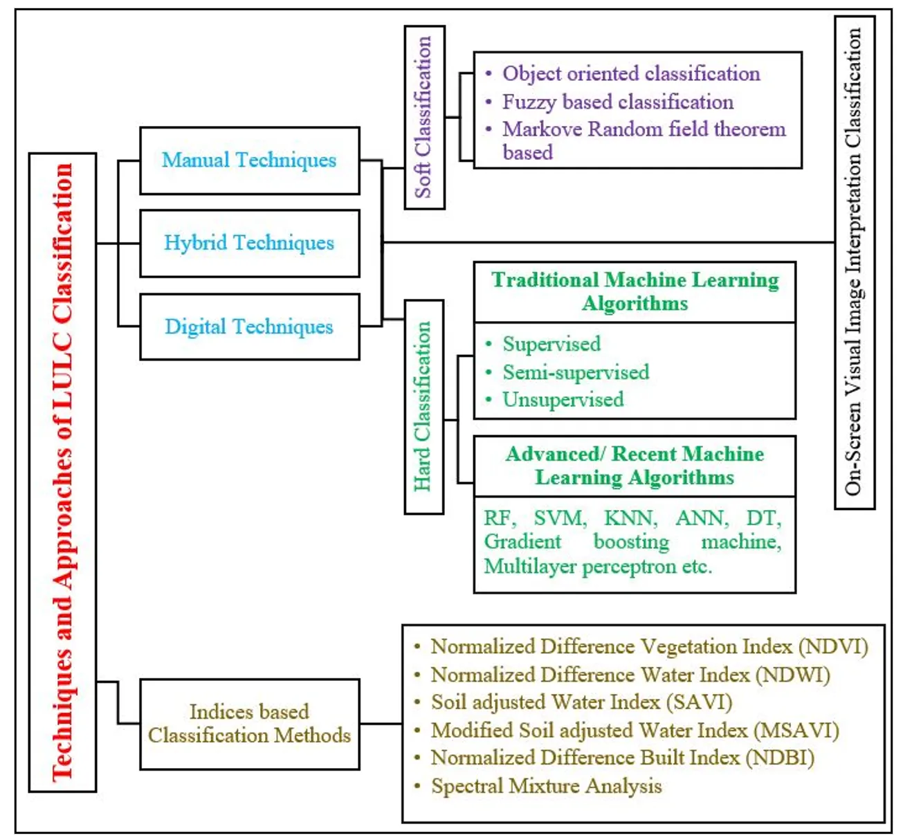
Visual image interpretation is one of the traditional classification approach which has been used extensively in terms of obtaining land use land cover mapping but as it is time consuming approach the new advanced image processing approaches have been developed such as unsupervised algorithms (
i.e., ISODATA, K-mean algorithm, Affinity Propagation (AP), fuzzy c-means algorithm
etc.), supervised algorithms such as maximum likelihood, machine learning algorithms
i.e., artificial network (ANN), k-Nearest Neighbors (KNN), decision tree (DT), support vector machines (SVM) and random forest (RF) and deep learning algorithms
i.e., CNN
etc. [
6,
7]. Thus, several studies have been conducted using machine learning algorithms to compare their accuracies to determine which algorithm is better among themselves or other algorithms. LULC classification is incomplete. shows different techniques and approaches for LULC classification in Remote Sensing and Geographic Information System (GIS).
This particular study aims to understand the results of LULC using different machine learning algorithms [
8,
9,
10,
11,
12] and visual image interpretation algorithm. This study also includes the assessment of accuracy of all the algorithms along with their comparison with each other. Several studies have been implemented to determine which classification algorithm is best for land use and land cover classification. Limited studies have been conducted, and a comparison of machine learning algorithms with visual interpretation has not yet been conducted using Sentinel-2 satellite data spatially in the Jalandhar district of Punjab, India. The objectives are to evaluate the performance of six classifiers,
i.e., RF, Gradient boosting, SVM, KNN, multilayer perceptron along with visual interpretation and evaluate the best classification accuracy of the classification results. This study highlights the comparative analysis of traditional approaches like visual interpretation by an expert for delineating different LULC classes vs. the established ML algorithms,
i.e., RF, Gradient boosting, SVM, KNN, and multilayer perceptron, which have demonstrated promising results in similar studies. The study also emphasizes the importance of visual interpretation for a more accurate LULC map at a regional level; meanwhile, leveraging advancements in ML algorithmsin a hybrid approach will enhance the accuracy in many-fold. This study Results of this research can be helpful for many upcoming studies to understand the performance of traditional and modern classifiers, to make the selection of an approach to be used for their research.
. Different Techniques and Approaches for LULC Classification.
2. Materials and Methods
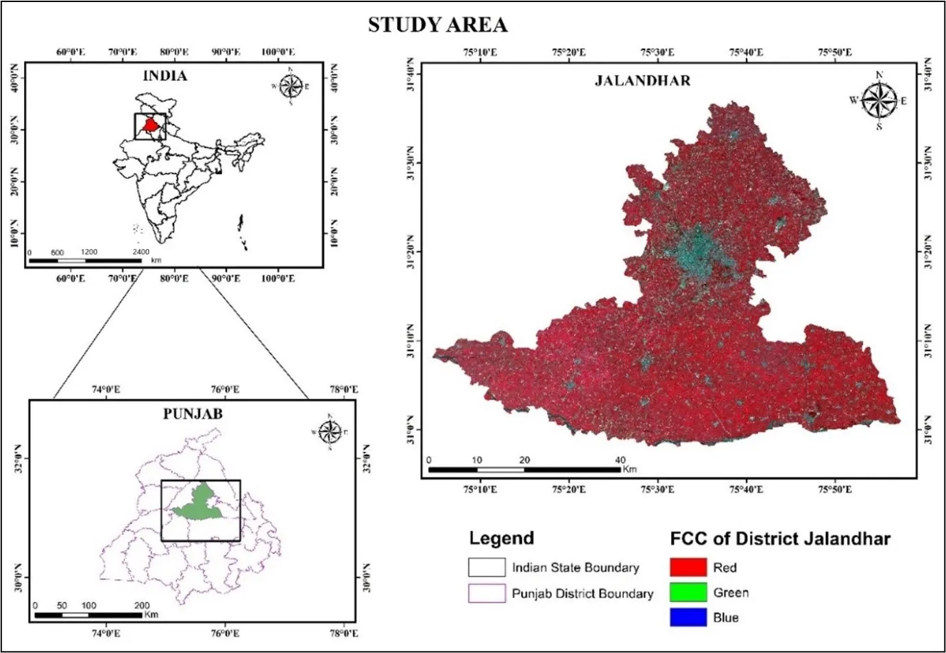
2.1. Study Area
The current study was conducted in the Jalandhar district of Punjab, India, as shown in . District Jalandhar is a central part of the Punjab, and it falls in the Doab region of the Punjab. It lies between the North latitude 30°8′ and 31°37′ and East longitude 75°08′ and 76°18′. In the southern part, it is bounded by the Sutlej River, which separates it from the Firozpur district of Punjab.
On the north-west, Kapurthala district intervenes between the Jalandhar territory and Bias River, and it shares its boundaries with Hoshiarpur district on the north-east. Sutlej River is the major natural drainage channel in the state, which is observed in the area. The average annual rainfall received by the district is about 703 mm and about 70% of the overall rainfall is during monsoon from the month of July to September (CGWB 2016, 2018 ) & [
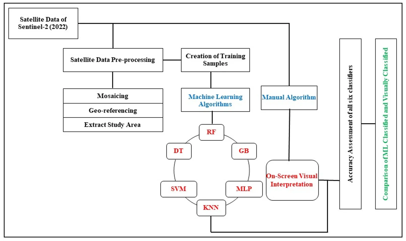
13]. District faced temperature from the range of 5 °C in winters to 45 °C in summer. As it can be seen in study area is Agriculture dominant where Paddy and Wheat are the major cereals grown in Kharif and Rabi season respectively. Overall flow chart of methodology is shown in .
. Framework of Methodology.
To conduct this study, the open-source high spatial resolution multi-spectral Sentinel-2 satellite data has been used and acquired on 4 October 2022. Satellite data is acquired and downloaded from the open-source Copernicus hub. Sentinel-2A and Sentinel-2B were launched using the European launcher VEGA. The Copernicus Sentinel-2 mission is made up of two polar-orbiting satellites that are aligned in the same sun-synchronous orbit at 180 degrees apart. A satellite image of the study area can be seen in , and specifications of satellite data are given in .
.
Specifications of Sentinel-2 Satellite Data.
| Sensor |
Bands |
Wavelength (µm) |
Resolution (m) |
Swath (km) |
| Sentinel-2A |
B1—Coastal aerosol |
0.443 |
60 |
290 |
| B2—Blue |
0.49 |
10 |
| B3—Green |
0.56 |
10 |
| B4—Red |
0.665 |
10 |
| B5—Vegetation Red Edge |
0.705 |
20 |
| B6—Vegetation Red Edge |
0.74 |
20 |
| B7—Vegetation Red Edge |
0.783 |
20 |
| B8—NIR |
0.842 |
10 |
| B8A—Vegetation Red Edge |
0.865 |
20 |
| B9—Water vapour |
0.945 |
60 |
| B10—SWIR—Cirrus |
1.375 |
60 |
| B11—SWIR |
1.61 |
20 |
| B12—SWIR |
2.19 |
20 |
2.3. Satellite Data Pre-Processing
Pre-processing of any satellite data is one of the important steps which needs to be taken care of, as it helps to remove noise and enhance the quality of the satellite data to better identify land use and land cover identification and classification. Before using the data, it is mosaicked and Geo-referenced. Satellite data was pre-processed using ArcGIS and ERDAS imagine software. Study area was clipped as per the district boundary as the last step before applying any classification algorithm.
2.4. LULC Classification Scheme and Training Samples
For running machine learning algorithms training samples are very much required. In this study different training samples were created as per our five major LULC classes
i.e., agriculture, built-up, plantation, waterbody and fallow & other.
Training samples were generated manually based on image interpretation elements, also called photo elements, and ancillary data such as maps and ground observations, were used to identify the land cover classes. A total of 750 training samples have been created, as shown in . These samples were selected from diverse parts of the study area to reflect intra-class variability and ensure better generalization by the ML classifiers. Once digitized, the training polygons were exported in shapefile format and used to extract pixel values from the relevant Sentinel-2 bands. The number and distribution of training samples can also affect the classification accuracy, which is why the number of training samples of all LULC classes was the same.
.
LULC Classes and Training Samples.
| S/N |
LULC Classes |
Description of Classes |
Number of Training Samples |
| 1 |
Agriculture |
Cropland |
150 |
| 2 |
Built-up |
Residential, commercial, industrial, transport |
150 |
| 3 |
Plantation |
Orchids, roadside trees etc. |
150 |
| 4 |
Waterbody |
Natural (Lake, River) and manmade |
150 |
| 5 |
Fallow & Other |
Open fields, barren, rocks, wasteland etc. |
150 |
| Grand Total |
750 |
The image-derived pixel samples were standardized through feature scaling, and then the dataset was split using a 70:30 ratio for training and validation, respectively. Care was taken to apply stratified sampling so that the proportion of each class remained balanced across both subsets.
2.5. Algorithms Used for LULC Classification
To classify LULC in the study area, a total of six algorithms are used, and these are divided into two categories,
i.e., Machine Learning Algorithms (RF, SVM, KNN, DT, GB and MLP) [
14,
15,
16,
17,
18,
19] and Visual Image Interpretation Algorithm and all algorithms used in this study are discussed below in
.
.
Description of all six Algorithms used for the study.
| S/N |
Algorithms |
Description of Algorithms |
| 1 |
Random Forest (RF) |
Random forests are an ensemble learning technique that combines multiple/random decision trees to generate predictions. To apply RF, you need to set up the number of features (mtry) and the number of trees (ntree). Because it can handle large and complex datasets and provides outstanding classification accuracy, it is quite popular among researchers for LULC classification. A majority vote is used to assign classes. |
| 2 |
Support Vector Machine (SVM) |
Support vector machines, or SVMs, create a model that divides the classes into a hyperplane by optimizing the margin between them. But binary classification was their first goal. Due to its excellent accuracy and low training cost, this technique is also well-liked by researchers studying LULC classification. |
| 3 |
K-Nearest Neighbor (KNN) |
After storing all the existing examples, a specific type of instance-based learning model, known as a KNN, classifies new instances based on similarity measurements. The distance fractions are utilized to identify the samples that are closest to the unknown samples, and the KNN class attributes are computed using the average of the response variables. (Noi and Kappas, 2017). |
| 4 |
Gradient Boosting (GB) |
This approach combines multiple weak models, like decision trees, to create a powerful model. It iteratively creates new models and then fixes the shortcomings of previous models (a process called boosting) using that training data. Xtreme Gradient Boosting, sometimes known as XGBoost, is an improved gradient boosting method. Due to its exceptional performance and efficacy, it is widely used in numerous applications, such as regression and classification. |
| 5 |
Multilayer Perceptron (MLP) |
For LULC classification, this method, also known as an artificial neutral network is frequently used. Its construction consists of three layers: the output layer, the hidden layer, and the input layer. It requires many training samples because of its high computing requirements. |
| 6 |
Decision Tree (DT) |
For LULC classification, this method—also known as an artificial neutral network—is frequently used. Its construction consists of three layers: the output layer, the hidden layer, and the input layer. It requires many training samples because of its high computing requirements. |
| 7 |
Visual Interpretation |
A manual on-screen visual interpretation algorithm is used to digitize different LULC classes that are present in the research region. Interpretation keys, or more precisely, the photo elements i.e., size, shape, color, texture, association, shadow, tone, site, and pattern are the basis of the digitization. A 1:6000 scale is used to map each class in this investigation. |
2.6. Data Processing
Model development and classification were performed using Scikit-learn, an open-source machine learning toolkit in Python. Each classifier was configured based on prior research and empirical testing. The RF model was constructed with 300 decision trees, which provided a balance between performance and computational cost. The DT classifier, on the other hand, employed a maximum depth of 10 to prevent overfitting while retaining classification sensitivity. The SVM was run using a linear kernel, which is well-suited for datasets with many features and records. A cost parameter (C) of 10 was used to control the trade-off between margin maximization and classification accuracy. For GB, 100 estimators with a default learning rate of 0.1 yielded optimal results during cross-validation. The KNN classifier operated with k = 5, a standard setting for minimizing classification noise while maintaining model responsiveness. The MLP was configured with a single hidden layer comprising 100 neurons, utilizing ReLU activation and the Adam optimizer [
20,
21,
22,
23,
24].
In parallel with the machine learning-based classification, a manual visual interpretation of Sentinel-2 imagery was carried out within ArcGIS Pro to produce an LULC map. This method relies on human expertise to identify and delineate land cover classes by visually analyzing spatial, spectral, and contextual information from satellite imagery. The interpretation was based on key/photo elements such as tone, texture, pattern, shape, size, shadow, site, and association. Although this method requires considerable time and relies on expert judgment, it enables detailed spatial mapping and integrates contextual understanding of the landscape. This manually interpreted LULC map was subsequently used as a reference for validating and comparing the results obtained from machine learning-based classifications.
2.7. Accuracy Assessment of Algorithms
The accuracy assessment of all six ML classifiers and the visual interpretation method was evaluated using statistical criteria. A confusion matrix is a table that is used to evaluate the performance of a machine learning algorithm for a classification task. It compares the predicted class labels with the true class labels and provides counts of the correct and incorrect predictions for each class. Overall accuracy, user’s accuracy (Precision), producer’s accuracy (Recall or Sensitivity), Kappa coefficient, and F1-score were utilized. Precision is a measure of the accuracy of the classifier when it predicts a positive class. Recall is a measure of the classifier’s ability to detect the positive class. High recall indicates that the classifier is good at detecting all positive instances. The F1 score is the harmonic mean of the producer and user accuracy. The better the portrayal, the higher the score. Overall accuracy is the percentage of correct predictions made by the classifier. It describes how well the classifier performed for each class that was present in the categorized image. Kappa statistics considers adjusting for accuracy depending on chance. It is important to evaluate classification accuracy to determine how well the classifier was able to differentiate between the many classes included in the image. The classified image was tested for this investigation using testing samples and the classified image. The confusion matrix is used in the equation below to calculate the overall accuracy of the categorized image. To compute this,
Equation (1),
Equation (2),
Equation (3),
Equation (4) and
Equation (5) were used, which are given below:
where,
TP = True Positive
FP = False Positive
FN = False Negative
i is the number of classes
N is the total number of classified values
$$m_{i , i}$$ is the number of values of the correct class
$$C_{i}$$ is the total number of predicted values in class I
$$G_{i}$$ is the total number of correct values in class I.
3. Results and Discussion
3.1. LULC Classification Comparison with Visual Image Interpretation
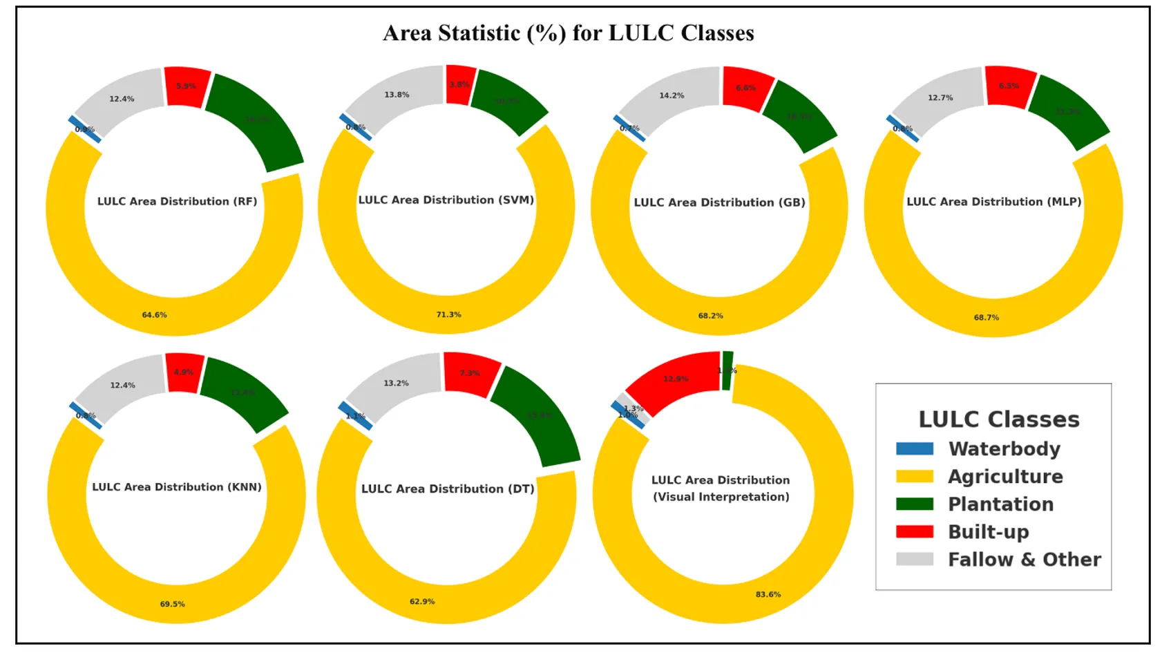
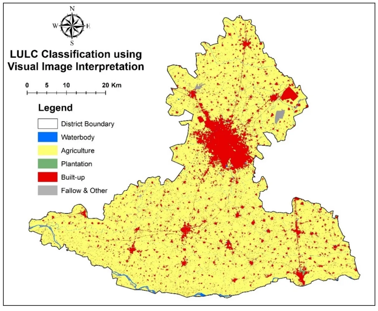
A range of machine learning algorithms, RF, SVM, GB, MLP, KNN and DT were applied for LULC classification, and their outputs were evaluated against visual interpretation, used here as a reference and shown in
and
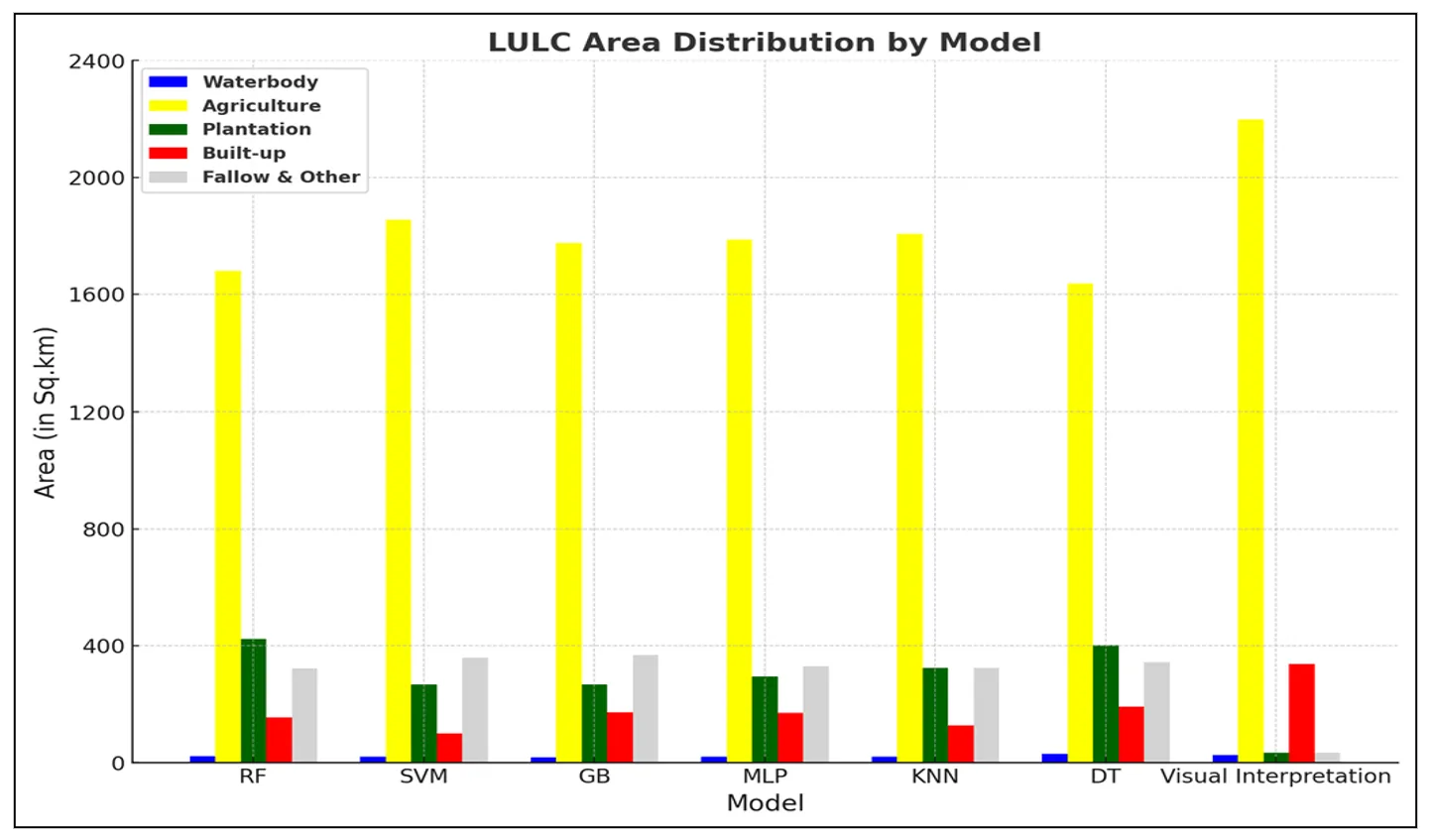
. Among all categories, agricultural land dominated. While visual interpretation showed 83.58% of the area as agricultural, all machine learning models underestimated this extent. SVM came closest with 71.31%, followed by KNN (69.45%), MLP (68.68%), and GB (68.22%). RF and DT showed the lowest estimations at 64.58% and 62.92%, respectively. These differences suggest that automated classifiers may misclassify agricultural parts as plantation or fallow land.
. Area Statistics in %age of LULC classification using ML Algorithms and Visual Interpretation.
In terms of Plantation, all models significantly overclassified this category compared to visual interpretation, which identified only 1.31% plantation area. RF (16.24%) and DT (15.41%) recorded the highest values, while SVM and GB were comparatively lower, though still much higher than the reference. For the Built-up class, Visual Interpretation estimated 12.86%, and the closest approximations came from DT (7.32%), GB (6.6%), and MLP (6.53%). On the other hand, SVM (3.8%) and KNN (4.89%) reported lower built-up coverage, suggesting potential confusion with fallow or bare areas. A notable discrepancy was found in the Fallow & Other category. While visual interpretation indicated only 1.27%, machine learning outputs ranged much higher. GB (14.16%), SVM (13.79%), and DT (13.21%) exhibited substantial overestimation, likely due to misclassification of marginal agricultural areas. Waterbody classification showed relatively strong consistency across methods. The reference estimate was 0.99%, while models produced values between 0.71% (GB) and 1.13% (DT), indicating a relatively high level of agreement and reliable identification of this class.
.
Area Statistics of LULC classes from ML Algorithms and Visual Interpretation.
| Model/Class |
Waterbody |
Agriculture |
Plantation |
Built-Up |
Fallow & Other |
Area
(Sq.km) |
Area
(%) |
Area (Sq.km) |
Area
(%) |
Area (Sq.km) |
Area (%) |
Area (Sq.km) |
Area (%) |
Area (Sq.km) |
Area (%) |
| RF |
22.52 |
0.87 |
1680.01 |
64.58 |
422.55 |
16.24 |
153.49 |
5.9 |
322.3 |
12.39 |
| SVM |
20.25 |
0.78 |
1854.97 |
71.31 |
268.11 |
10.31 |
98.81 |
3.8 |
358.74 |
13.79 |
| GB |
18.34 |
0.71 |
1774.26 |
68.22 |
268.13 |
10.31 |
171.76 |
6.6 |
368.38 |
14.16 |
| MLP |
19.86 |
0.76 |
1786.32 |
68.68 |
295.01 |
11.34 |
169.81 |
6.53 |
329.87 |
12.68 |
| KNN |
20.59 |
0.79 |
1806.83 |
69.45 |
323.35 |
12.43 |
127.3 |
4.89 |
322.81 |
12.41 |
| DT |
29.29 |
1.13 |
1636.84 |
62.92 |
400.93 |
15.41 |
190.37 |
7.32 |
343.45 |
13.21 |
| Visual Interpretation |
26.05 |
0.99 |
2197.93 |
83.58 |
34.32 |
1.31 |
338.23 |
12.86 |
33.46 |
1.27 |
A detailed assessment of classified land use/land cover outputs revealed notable differences in spatial estimates among the machine learning models and the reference data. The corresponding area statistics are detailed in
and
while the classified outputs for each model are illustrated in
,
,
,
,
,
and
.
. Area Distribution of LULC classes based on ML Algorithms and Visual Interpretation.
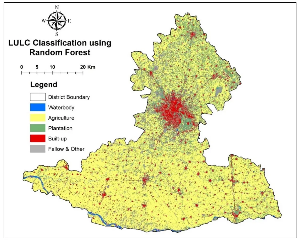
. LULC Classification using Random Forest.
. LULC Classification using Support Vector Machine Learning.
. LULC Classification using Gradient Boosting.
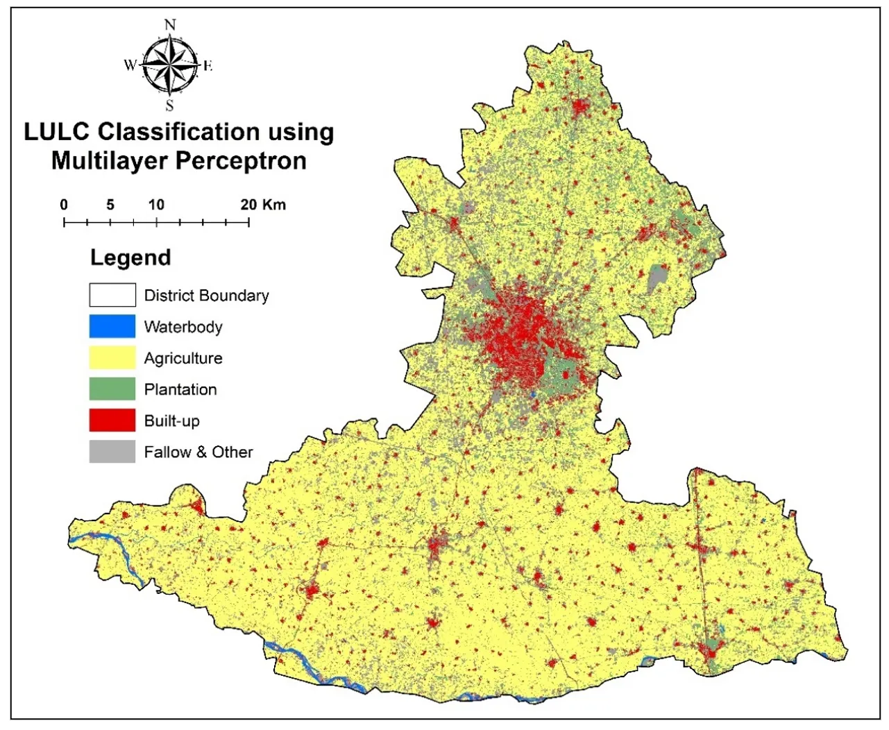
. LULC Classification using Multilayer Perceptron.
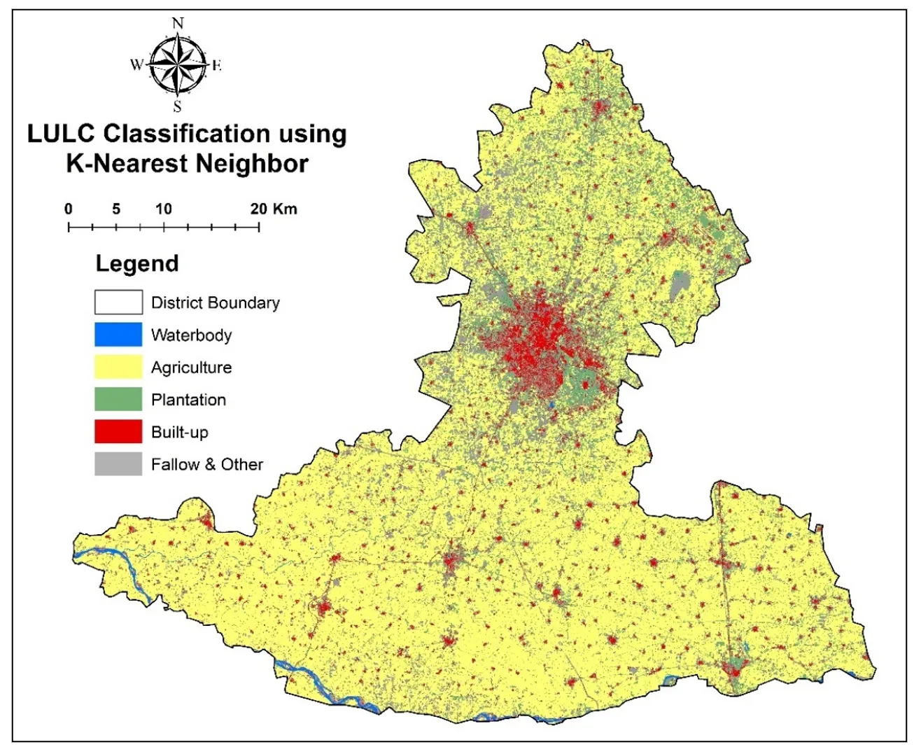
. LULC Classification using K-Nearest Neighbor.
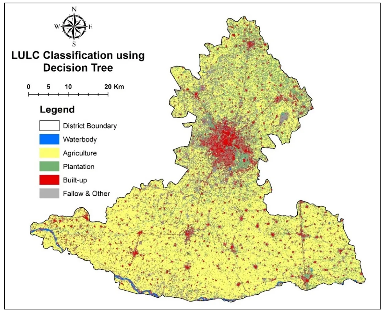
. LULC Classification using Decision Tree.
. LULC Classification using Visual Image Interpretation.
The agriculture category, identified as 2197.93 sq.km in the reference map, was consistently underestimated by all models. The highest estimate came from SVM (1854.97 sq.km), followed by KNN (1806.83 sq.km) and MLP (1786.32 sq.km). This gap suggests misclassification with nearby land classes such as plantations or fallow land. Plantation areas were significantly overestimated across models compared to the reference value of 34.32 sq.km. Predictions ranged from 268.11 sq.km (SVM) to 422.55 sq.km (RF), indicating frequent confusion with other vegetation types. For built-up land, the visual interpretation mapped 338.23 sq.km, while models like DT (190.37 sq.km) and GB (171.76 sq.km) provided the closest estimates. SVM (98.81 sq.km) and KNN (127.3 sq.km) notably underestimated this class, pointing to difficulties in detecting developed areas. In the fallow and other classes, the reference area was just 33.46 sq.km, but machine learning outputs were much higher up to 368.38 sq.km (GB). This overclassification highlights challenges in distinguishing barren land from inactive agricultural plots. Finally, waterbodies showed the most consistent classification, with estimates ranging between 18.34 sq.km (GB) and 29.29 sq.km (DT), compared to the reference value of 26.05 sq.km.
3.2. Accuracy Assessment
The evaluation of classification performance was carried out using key accuracy metrics such as overall accuracy, kappa coefficient, producer accuracy, and user accuracy. A detailed breakdown of these results for each machine learning model and visual interpretation method is presented in
,
,
,
,
,
and
, highlighting how effectively each approach classified the major LULC categories. A comparative evaluation of classification models revealed that GB delivered the best performance, achieving an overall accuracy of 95.0% and a kappa coefficient of 0.94. Its high precision across all land use classes and strong handling of complex spatial patterns made it the most robust model in this study. RF model followed closely, with an accuracy of 94.2% and a kappa value of 0.92. RF’s ensemble-based structure enabled stable results, although it was slightly less accurate than GB in certain transitional zones. The SVM also performed well, reaching an accuracy of 93.8% and a kappa value of 0.91. It effectively classified dominant land types like water and agriculture, but showed a minor drop in accuracy for urban categories. MLP yielded 91.5% accuracy and a kappa of 0.89, performing consistently across classes but facing challenges in more complex or mixed land covers such as plantation and built-up areas.
Meanwhile, the KNN model recorded 89.7% accuracy and a kappa value of 0.86, performing reasonably in simpler classes but showing limitations in distinguishing spectrally similar land types. The DT model had the lowest classification performance among machine learning methods, with an accuracy of 87.5% and a kappa of 0.84, primarily due to overfitting and reduced capacity to generalize across varied landscape patterns. In comparison, visual interpretation achieved a moderate accuracy of 90.1% with a kappa value of 0.88. While not as statistically precise as some machine learning techniques, its strength lies in its contextual recognition and cost-effective application, making it a practical tool for operational land cover assessments.
.
Accuracy assessment of LULC classification using RF.
| LULC Classes |
Producer Accuracy (Recall) |
User Accuracy (Precision) |
| Water |
0.96 |
0.95 |
| Agriculture |
0.94 |
0.93 |
| Plantation |
0.93 |
0.92 |
| Built-Up |
0.9 |
0.91 |
| Fallow & Others |
0.94 |
0.93 |
| Overall Accuracy |
94.20% |
|
| Kappa |
0.92 |
|
.
Accuracy assessment of LULC classification using SVM.
| LULC Classes |
Producer Accuracy (Recall) |
User Accuracy (Precision) |
| Water |
0.95 |
0.94 |
| Agriculture |
0.93 |
0.92 |
| Plantation |
0.92 |
0.91 |
| Built-Up |
0.88 |
0.89 |
| Fallow & Others |
0.93 |
0.92 |
| Overall Accuracy |
93.80% |
|
| Kappa |
0.91 |
|
.
Accuracy assessment of LULC classification using GB.
| LULC Classes |
Producer Accuracy (Recall) |
User Accuracy (Precision) |
| Water |
0.98 |
0.97 |
| Agriculture |
0.96 |
0.95 |
| Plantation |
0.95 |
0.94 |
| Built-Up |
0.93 |
0.92 |
| Fallow & Others |
0.96 |
0.95 |
| Overall Accuracy |
95.00% |
|
| Kappa |
0.94 |
|
.
Accuracy assessment of LULC classification using MLP.
| LULC Classes |
Producer Accuracy (Recall) |
User Accuracy (Precision) |
| Water |
0.92 |
0.91 |
| Agriculture |
0.91 |
0.9 |
| Plantation |
0.9 |
0.89 |
| Built-Up |
0.88 |
0.87 |
| Fallow & Others |
0.91 |
0.9 |
| Overall Accuracy |
91.50% |
|
| Kappa |
0.89 |
|
.
Accuracy assessment of LULC classification using KNN.
| LULC Classes |
Producer Accuracy (Recall) |
User Accuracy (Precision) |
| Water |
0.9 |
0.89 |
| Agriculture |
0.89 |
0.88 |
| Plantation |
0.88 |
0.87 |
| Built-Up |
0.85 |
0.86 |
| Fallow & Others |
0.89 |
0.88 |
| Overall Accuracy |
89.70% |
|
| Kappa |
0.86 |
|
.
Accuracy assessment of LULC classification using DT.
| LULC Classes |
Producer Accuracy (Recall) |
User Accuracy (Precision) |
| Water |
0.88 |
0.87 |
| Agriculture |
0.87 |
0.86 |
| Plantation |
0.86 |
0.85 |
| Built-Up |
0.82 |
0.83 |
| Fallow & Others |
0.87 |
0.86 |
| Overall Accuracy |
87.50% |
|
| Kappa |
0.84 |
|
.
Accuracy assessment of LULC classification using Visual Interpretation.
| LULC Classes |
Producer Accuracy (Recall) |
User Accuracy (Precision) |
| Water |
0.91 |
0.9 |
| Agriculture |
0.9 |
0.89 |
| Plantation |
0.88 |
0.87 |
| Built-Up |
0.86 |
0.85 |
| Fallow & Others |
0.9 |
0.89 |
| Overall Accuracy |
90.10% |
|
| Kappa |
0.88 |
|
Among all models assessed for LULC classification, GB showed the highest reliability and accuracy, maintaining consistent performance across all land cover categories. RF and SVM also delivered strong results, demonstrating good generalization across diverse land types. MLP and KNN offered moderate accuracy but showed some sensitivity to complex or mixed patterns. DT recorded the lowest accuracy among the ML models, reflecting its limitations in handling heterogeneous land cover. While visual interpretation was less accurate compared to the ML-based approaches, its simplicity, real-time adaptability, and ease of use make it a practical option for field-level applications, despite some difficulties in classifying intricate patterns.
4. Conclusions
This study comprehensively assessed the performance of various machine learning models for land use/land cover (LULC) classification from remote sensing data, highlighting their comparative effectiveness. Gradient Boosting (GB) emerged as the top performer, achieving the highest overall accuracy (95.0%) and a kappa value of 0.94. This model successfully delineated major classes, with agricultural land covering approximately 1774.26 sq. km and built-up areas spanning 171.76 sq. km. Random Forest (RF) and Support Vector Machine (SVM) followed closely, which demonstrated robust generalization capabilities with accuracy of 94.2% and 93.8%, respectively. This pattern underscores the superior classification power of ensemble and kernel-based algorithms for complex, high-dimensional datasets. A notable observation was the consistent underestimation of certain LULC classes. Agricultural land, visually interpreted to be the most extensive class (2197.93 sq. km), was significantly underestimated by all models, particularly by GB and Multi-Layer Perceptron (MLP). This indicates a challenge in accurately distinguishing between spectrally similar or heterogeneous agricultural sub-types. Conversely, plantation and fallow lands were consistently overestimated, a finding that points to spectral confusion with adjacent vegetation categories. In contrast, water bodies were classified with high precision across all models, confirming the effectiveness of these algorithms in identifying spectrally distinct features. While visual interpretation had a slightly lower accuracy (90.1%, kappa 0.88), its utility extends beyond numerical performance. Its operational simplicity and adaptability for field validation make it an invaluable complementary tool for fine-tuning models and resolving classification ambiguities. This research underscores that integrating advanced machine learning classifiers, especially GB, RF, and SVM, significantly improves the accuracy and detail of LULC mapping. The findings emphasize that successful LULC classification hinges not only on selecting the most robust algorithm but also on meticulous validation and strategic post-classification refinement to address class-specific spectral challenges. The results provide crucial evidence for leveraging machine learning to support data-driven land management and planning, especially in diverse and dynamic environments.
5. Limitations of the Study & Future Scope
Despite its significant findings, this study has several limitations that provide avenues for future research. One key constraint was the reliance on a single-sensor dataset (Sentinel-2), which may not fully capture the spectral complexity of certain land cover types. The limited spectral and temporal resolution of this data may have contributed to the observed spectral confusion between classes, such as agricultural land and fallow land. Furthermore, the spatial resolution of the imagery might be too coarse for accurately identifying highly fragmented or small-scale LULC features, which is particularly relevant in heterogeneous landscapes. Another limitation is the static nature of the classification, as the analysis was based on a single-point-in-time image. This approach overlooks the dynamic changes in land use and land cover, which can vary significantly with seasons (e.g., crop cycles) or land management practices. The extensive ground truth data is not collected for this study to validate the ground-level LULC information, but validated visually and by using open-source available very high resolution imagery like Google Earth and its archival. The selection of machine learning models was limited to a specific set of commonly used classifiers; other advanced architectures, such as deep learning models like Convolutional Neural Networks (CNNs), were not included.
Based on these limitations, several pathways for future research are recommended. Future studies should explore the integration of multi-sensor and multi-temporal data. Combining optical imagery from satellites like Sentinel-2 with radar data (e.g., Sentinel-1) could enhance class reparability, particularly for distinguishing crops and built-up areas. Incorporating time-series analysis would enable the detection of LULC changes and provide a more comprehensive understanding of land dynamics. Deep learning models, especially CNNs and U-Net architectures, should be investigated for their ability to leverage spatial and contextual information, which is often more effective in handling complex LULC patterns than traditional pixel-based classifiers.
Furthermore, future work should focus on improving the classification of spectrally mixed pixels through advanced techniques like spectral unmixing. This could help resolve the confusion observed between classes like agriculture and fallow land. The application of active learning frameworks could also be beneficial, allowing models to iteratively request ground truth data for the most uncertain areas, thereby optimizing the data collection process and improving accuracy in challenging regions. Finally, future studies should consider transferability analysis to assess how the best-performing models from this study perform when applied to different geographic regions with varying ecological and land-use characteristics. This would validate the robustness and generalizability of the models, moving toward more scalable and operational LULC mapping solutions.
Statement of the Use of Generative AI and AI-Assisted Technologies in the Writing Process
During the preparation of this manuscript, the authors used AI Tools to assist with language editing and grammar refinement. All content was subsequently reviewed, revised, and approved by the authors, who take full responsibility for the final version of the manuscript.
Acknowledgments
The authors would like to thank National Remote Sensing Centre (NRSC) for providing and facilitating all required resources.
Author Contributions
Conceptualization, D.K.B. and A.D.; Methodology, D.K.B. and A.D.; Formal Analysis, D.K.B. and A.D.; Data Curation, A.D.; Investigation, A.D.; Writing—Original Draft Preparation, A.D.; Writing—Review & Editing, D.K.B., A.D., G.S. and R.K.; Supervision, G.S. and R.K.; Project Administration, G.S. and R.K.; Ground Truth Collection and Analysis, A.D.
Ethics Statement
Not applicable.
Informed Consent Statement
Not applicable.
Data Availability Statement
Data will be made available on request.
Funding
This research received no external funding.
Declaration of Competing Interest
The authors declare that they have no known competing financial interests or personal relationships that could have appeared to influence the work reported in this paper.
References
-
1.
Anderson JR. A Land Use and Land Cover Classification System for Use with Remote Sensor Data; US Government Printing Office: Washington, DC, USA, 1976; Volume 964.
-
2.
Ahire V, Behera DK, Saxena MR, Patil S, Endait M, Poduri H. Potential landfill site suitability study for environmental sustainability using GIS-based multi-criteria techniques for nashik and environs.
Environ. Earth Sci. 2022,
81, 178. doi:10.1007/s12665-022-10295-y.
[Google Scholar]
-
3.
Behera DK, Saxena MR, Ravi Shankar G. Decadal Land use and Land Cover Change Dynamics in East Coast of India-Case Study on Chilika Lake.
Indian. Geogr. J. 2017,
92, 73–82.
[Google Scholar]
-
4.
Behera DK, Pujar GS, Kumar R, Singh SK. A Comprehensive Approach Towards Enhancing Land Use Land Cover Classification Through Machine Learning and Object-Based Image Analysis.
J. Indian Soc. Remote Sens. 2024,
53, 731–749. doi:10.1007/s12524-024-01997-w.
[Google Scholar]
-
5.
Behera DK, Kumari A, Kumar R, Modi M, Singh SK. Assessment of Site Suitability of Wastelands for Solar Power Plants Installation in Rangareddy District, Telangana, India. In Ecological Footprints of Climate Change: Adaptive Approaches and Sustainability; Springer International Publishing: Cham, Switzerland, 2023. doi:10.1007/978-3-031-15501-7_22.
-
6.
Behera DK, Ramsankaran R, Pujar GS, Kumar R, Sreenivas K. A Class-balanced Cost Driven Deep Learning Approach for Efficient Land Use Land Cover Classification using Remote Sensing Data. In Proceedings of the 2024 IEEE India Geoscience and Remote Sensing Symposium (InGARSS), Goa, India, 2–5 December 2024; pp. 1–4, doi:10.1109/InGARSS61818.2024.10983963.
-
7.
Bhosle K, Musande V. Evaluation of Deep Learning CNN Model for Land Use Land Cover Classification and Crop Identification Using Hyperspectral Remote Sensing Images.
J. Indian. Soc. Remote Sens. 2019,
47, 1949–1958. doi:10.1007/s12524-019-01041-2.
[Google Scholar]
-
8.
Chachondhia P, Shakya A, Kumar G. Performance evaluation of machine learning algorithms using optical and microwave data for LULC classification.
Remote Sens. Appl. Soc. Environ. 2021,
23, 100599. doi:10.1016/j.rsase.2021.100599.
[Google Scholar]
-
9.
Ebrahimy H, Mirbagheri B, Matkan AA, Azadbakht M. Effectiveness of the integration of data balancing techniques and tree-based ensemble machine learning algorithms for spatially-explicit land cover accuracy prediction.
Remote Sens. Appl. Soc. Environ. 2022,
27, 100785. doi:10.1016/j.rsase.2022.100785.
[Google Scholar]
-
10.
Günen MA. Performance comparison of deep learning and machine learning methods in determining wetland water areas using EuroSAT dataset.
Environ. Sci. Pollut. Res. 2022,
29, 21092–21106. doi:10.1007/s11356-021-17177-z.
[Google Scholar]
-
11.
Jamali A. Evaluation and comparison of eight machine learning models in land use/land cover mapping using Landsat 8 OLI: A case study of the northern region of Iran.
SN Appl. Sci. 2019,
1, 1–11. doi:10.1007/s42452-019-1527-8.
[Google Scholar]
-
12.
Kavhu B, Eric Mashimbye Z, Luvuno L. Characterising social-ecological drivers of landuse/cover change in a complex transboundary basin using singular or ensemble machine learning.
Remote Sens. Appl. Soc. Environ. 2022,
27, 100773. doi:10.1016/j.rsase.2022.100773.
[Google Scholar]
-
13.
Kumar N, Singh VG, Singh SK, Behera DK, Gašparović M. Modeling of land use change under the recent climate projections of CMIP6: a case study of Indian river basin.
Environ. Sci. Pollut. Res. 2023,
30, 107219–107235. doi:10.1007/s11356-023-26960-z.
[Google Scholar]
-
14.
Kulithalai Shiyam Sundar P, Deka PC. Spatio-temporal classification and prediction of land use and land cover change for the Vembanad Lake system, Kerala: A machine learning approach.
Environ. Sci. Pollut. Res. 2021,
29, 86220–86236.
[Google Scholar]
-
15.
Lun NS, Chaudhary S, Ninsawat S. Assessment of Machine Learning Methods for Urban Types Classification Using Integrated SAR and Optical Images in Nonthaburi, Thailand.
Sustainability 2023,
15, 1051.
[Google Scholar]
-
16.
Rahman A, Abdullah HM, Tanzir MT, Hossain MJ, Khan BM, Miah MG, et al. Performance of different machine learning algorithms on satellite image classification in rural and urban setup.
Remote Sens. Appl. Soc. Environ. 2020,
20, 100410. doi:10.1016/j.rsase.2020.100410.
[Google Scholar]
-
17.
Rousset G, Despinoy M, Schindler K, Mangeas M. Assessment of deep learning techniques for land use land cover classification in southern new Caledonia.
Remote Sens. 2021,
13, 1–22. doi:10.3390/rs13122257.org/10.1007/s11356-021-17257-0.
[Google Scholar]
-
18.
Roy B. A machine learning approach to monitoring and forecasting spatio-temporal dynamics of land cover in Cox’s Bazar district, Bangladesh from 2001 to 2019.
Environ. Chall. 2021,
5, 100237. doi:10.1016/j.envc.2021.100237.
[Google Scholar]
-
19.
Saadeldin M, O’Hara R, Zimmermann J, Mac Namee B, Green S. Using deep learning to classify grassland management intensity in ground-level photographs for more automated production of satellite land use maps.
Remote Sens. Appl. Soc. Environ. 2022,
26, 100741. doi:10.1016/j.rsase.2022.100741.
[Google Scholar]
-
20.
Singh G, Pandey A. Evaluation of classification algorithms for land use land cover mapping in the snow-fed Alaknanda River Basin of the Northwest Himalayan Region.
Appl. Geomat. 2021,
13, 863–875. doi:10.1007/s12518-021-00401-3.
[Google Scholar]
-
21.
Singh RK, Singh P, Drews M, Kumar P, Singh H, Gupta AK, et al. A machine learning-based classification of LANDSAT images to map land use and land cover of India.
Remote Sens. Appl. Soc. Environ. 2021,
24, 100624. doi:10.1016/j.rsase.2021.100624.
[Google Scholar]
-
22.
Talukdar S, Singha P, Mahato S, Pal S, Liou YA, Rahman A. Land-use land-cover classification by machine learning classifiers for satellite observations-A review.
Remote Sens. 2020,
12, 1135. doi:10.3390/rs12071135.
[Google Scholar]
-
23.
Vali A, Comai S, Matteucci M. Deep learning for land use and land cover classification based on hyperspectral and multispectral earth observation data: A review.
Remote Sens. 2020,
12, 2495. doi:10.3390/RS12152495.
[Google Scholar]
-
24.
Woldemariam GW, Tibebe D, Mengesha TE, Gelete TB. Machine-learning algorithms for land use dynamics in Lake Haramaya Watershed, Ethiopia.
Model. Earth Syst. Environ. 2022,
8, 3719–3736. doi:10.1007/s40808-021-01296-0.
[Google Scholar]