Multi-Agent Reinforcement Learning for Optimal Operation of PV-ES-EV Microgrids

Microgrids, as autonomous systems integrating distributed generation, energy storage, charging infrastructure, and electrical loads, have emerged as a critical technical solution for accommodating renewable energy and enhancing power supply reliability. In China, the “dual carbon” strategy—a national policy framework targeting carbon emission peaking by 2030 and carbon neutrality by 2060—has been fully implemented nationwide to accelerate the country’s energy transition. Under this strategic context, the penetration rate of renewable energy, especially photovoltaic (PV) power, in distribution networks keeps growing. Nevertheless, the inherent intermittency of PV output and the stochastic characteristics of electric vehicle (EV) charging loads are mutually coupled, bringing dual uncertainties to the operation of microgrids. Microgrids typically exchange power with the main grid through a point of common coupling. During grid-connected operation, they can exploit peak-valley electricity price differences to reduce costs; during islanded operation, they must rely on local resources to supply critical loads. Achieving a dynamic balance between the pursuit of economic efficiency in grid-connected operation and the security assurance in islanded operation is the central challenge in microgrid energy management.

The problem of grid-connected microgrid optimization has been extensively studied in the academic literature. Conventional optimization methods mainly fall into two categories: mathematical programming and heuristic algorithms. Approaches such as Model Predictive Control (MPC) and Mixed Integer Linear Programming (MILP) can obtain optimal dispatch schemes when prediction information is accurate, by establishing precise system models [1,2]. However, these methods rely heavily on prediction accuracy and model parameters, making it difficult to adapt to the strong uncertainties on both the source and load sides. Heuristic algorithms, such as particle swarm optimization and genetic algorithms, alleviate modeling difficulties to some extent, but they suffer from slow convergence, a tendency to become trapped in local optima, and an inability to retain optimization knowledge for new scenarios [3,4].

From a regulatory perspective, the development of microgrids and distributed PV in China operates within a well-defined policy framework. The National Energy Administration (NEA) has issued a series of guidelines—such as the Administrative Measures for Grid-Connected Operation of Distributed Generation and the Trial Measures for Promoting the Construction of Grid-Connected Microgrids—that explicitly encourage the integration of distributed PV, energy storage, and controllable loads into local distribution networks. These regulations permit microgrids to trade electricity with the main grid under time-of-use tariffs and, crucially, mandate that microgrids possess the capability for intentional or unintentional islanding with adequate reserve margins to ensure the security of critical loads during grid disturbances. While the specific tariff structures and interconnection standards vary across jurisdictions (e.g., in parts of Latin America or Europe where feed-in tariffs and self-consumption rules differ substantially), the proposed dynamic weighting methodology is designed to be agnostic to the underlying tariff regime: the weight generation network learns to adapt its economic-autonomy trade-off from real-time price signals and system states, making the approach conceptually transferable to any liberalized electricity market with a time-varying price structure and islanding capability requirements.

In recent years, Deep Reinforcement Learning (DRL) has attracted considerable attention because it does not require precise modeling and excels at sequential decision-making problems [5,6]. Relevant studies have applied DRL to microgrid energy storage scheduling, EV charging/discharging control, and multi-energy complementary system optimization [7,8,9]. Among these, the Proximal Policy Optimization (PPO) algorithm, owing to its stable policy update mechanism and good convergence performance, has become one of the mainstream methods for addressing continuous action space optimization problems [10]. In microgrid scenarios, PPO has been validated as effective in handling uncertainties in renewable energy output and load demand, thereby reducing system operating costs [11,12].

In China, as microgrids scale up and the variety of internal unit types increases, the single-agent architecture faces challenges of the high state space dimensionality and declining decision-making efficiency. Multi-Agent Reinforcement Learning (MARL), which models different controllable units as independent agents, achieves coordinated optimization through the centralized training with decentralized execution paradigm [13,14]. In this paradigm, a global critic network utilizes full system-level information in the offline training phase to learn coordinated operation strategies, while in the online operation phase, each individual agent generates real-time dispatch decisions relying solely on local measurements, with no need for inter-agent communication or access to global system states. This design fits inherently with the standard operational requirements of power distribution systems, where each standalone controllable unit (such as energy storage inverters and EV charging devices) must respond autonomously to local signals, independent of a centralized controller. This also ensures full compliance with current grid codes, which explicitly require a distributed decision-making architecture and strict data privacy protection. Studies have shown that multi-agent architectures outperform single-agent approaches in microgrid scheduling, distributed energy management, and related fields [15,16]. Among them, Multi-Agent Proximal Policy Optimization (MAPPO) effectively handles collaborative decision-making among multiple agents while retaining the stability of PPO [17].

For multi-objective optimization, existing research mainly adopts two strategies: first, converting multiple objectives into a single objective through linear weighting, though the weight coefficients must be predetermined and remain fixed [18]; second, using Pareto-based multi-objective methods, which generate a Pareto front but still rely on operator preferences for final scheme selection [19]. Neither of these methods addresses the issue of dynamically adjusting weights according to system states. In fact, the dispatch strategy adopted during microgrid grid-connected operation directly affects resilience performance under islanded conditions, and there is strong coupling between the two [20]. This implies that there is a dynamic trade-off between the autonomy capacity reserved during grid-connected operation—namely, islanding preparedness—and the immediate economic benefits, with the optimal balance point shifting with electricity prices, energy storage state, PV output, and potential islanding risks.

Nevertheless, existing research still has the following shortcomings. First, multi-objective optimization weights are fixed and cannot adapt to the optimization focus according to real-time system states, making it difficult to make rational decisions when conflicts arise between peak electricity prices and insufficient storage. Second, the decision of electricity purchase/sale from the external grid is handled separately from internal dispatch, lacking a joint optimization mechanism. Third, the economic optimization of grid-connected operation and the autonomy preparedness for islanded conditions have not been effectively coordinated; most studies focus on a single operation mode and overlook the safety margin requirements when switching between modes.

To address these issues, this paper proposes a multi-agent proximal optimization coordination strategy for microgrids that incorporates dynamic autonomy weighting. The main contributions are as follows:

The remainder of this paper is organized as follows. Section 2 describes the microgrid system modeling and the dynamic autonomy weighting mechanism. Section 3 elaborates on the multi-agent collaborative optimization algorithm based on MAPPO. Section 4 validates the effectiveness of the proposed strategy through simulation experiments. Section 5 concludes the paper and discusses future work.

The microgrid system under study comprises four categories of flexible resources: photovoltaic generation units, battery energy storage systems, electric vehicle charging stations, and interruptible loads with differentiated priority levels. The system interfaces with the main grid through a point of common coupling, enabling operation in both grid-connected and islanded modes. The core task of microgrid energy management can be formalized as follows: at each dispatch interval t, based on the current system state $$S_t$$—which encompasses photovoltaic power forecasts, state of charge of the storage system, real-time charging power of charging stations, load demand, and time-of-use electricity prices—along with the system’s perception of islanding risk, a set of decision variables is determined. These comprise, on one hand, the dispatch scheme for internal controllable units $$U_t^{{\rm{internal}}}$$ (storage charging/discharging power, charging station regulation levels, and switching status of interruptible loads), and on the other hand, the optimal power exchange with the main grid $$P_t^{{\rm{grid}}}$$, both of which are determined at each time step.

This decision-making process inherently involves a fundamental trade-off. Pursuing economic benefits through aggressive participation in the electricity market may lead to an excessively low state of charge in the storage system and insufficient local reserve capacity, thereby compromising the microgrid’s ability to transition smoothly to islanded operation in the event of a grid fault. Conversely, over-reserving autonomous capacity increases operational costs and diminishes economic performance. The optimal balance point is not a fixed value; it shifts dynamically with fluctuations in electricity prices, energy storage status, photovoltaic power output, and the perceived risk of unintended islanding.

To tackle this core challenge, this paper puts forward a multi-agent collaborative optimization framework embedded with dynamic autonomy weights. The core design logic is twofold. First, controllable resources inside the microgrid are modeled as independent agents with standalone decision-making capabilities, to realize collaborative optimization via multi-agent reinforcement learning. Second, a lightweight neural network is introduced to generate dynamic weights for three core optimization objectives—operational economy, grid safety, and autonomy performance—according to the system’s real-time operating state, enabling the optimization priority to adapt flexibly to varying working conditions. The entire framework follows the classic centralized training with decentralized execution paradigm: full system-wide information is utilized during the training phase to learn coordinated control strategies, while in the execution phase, each agent generates real-time dispatch decisions relying solely on its local observable data. The detailed structure of the framework is illustrated as shown in Figure 1:

The decomposition of a microgrid into multiple agents stems from the recognition that different resources exhibit fundamentally distinct physical characteristics, coordination motivations, and response time scales. The photovoltaic agent’s coordination action—curtailment—involves a trade-off between electricity sales revenue and renewable energy utilization. The storage agent’s decisions require balancing immediate economic returns against the need to preserve reserve capacity for future islanding events. Charging stations, as controllable loads, must account for the welfare loss experienced by users when their charging demand is curtailed. Interruptible loads serve as a last-resort coordination measure for system operation, in which their switching actions directly incur corresponding compensation costs. By modeling such resources as independent individual agents, each agent can prioritize the optimization objectives most aligned with its own operational characteristics, while overall system-level coordination is realized via the coupling mechanism embedded in the global reward function.

The photovoltaic agent’s decision variable is the curtailment ratio. Its local observation space is deliberately constrained to information directly relevant to its decision:

where $$P_t^{{\rm{PV,max}}}$$ is the forecasted maximum available photovoltaic power (kW), and $${\lambda _t}$$ is the time-of-use electricity price (RMB/kWh). This design reflects the rationale that the photovoltaic agent does not need to perceive the status of other resources, as its decision depends only on how much power could be generated and the value of that power.

The action $$a_t^{{\rm{PV}}} \in [0,1]$$ is a continuous variable representing the curtailment ratio, with the actual grid-connected power determined by:

The operational constraint is $$0 \le P_t^{{\rm{PV,out}}} \le P_t^{{\rm{PV,max}}}$$. The local reward for the photovoltaic agent is defined as the negative of the opportunity cost of curtailment:

where $${\gamma _{{\rm{PV}}}}$$ is a curtailment penalty coefficient and $$\Delta t$$ is the dispatch interval (1 h). This reward structure discourages curtailment, with the penalty scaling linearly with the electricity price. Consequently, the agent is incentivized to minimize curtailment particularly during periods of high electricity prices, unless forced by technical constraints (e.g., reverse power flow limits or storage saturation). This aligns the local objective with the system-level goal of maximizing renewable energy revenue.

The battery energy storage agent serves as the cornerstone for power balance maintenance and islanding capability. Its local observation includes three key elements:

where $${\rm{SO}}{{\rm{C}}_t}$$ is the current state of charge expressed as a normalized value (0–1, with 1 corresponding to 100% capacity), $$P_t^{{\rm{BESS}}}$$ is the current charging/discharging power (kW), and $$\lambda _t$$ is the electricity price.

The action $$a_t^{{\rm{BESS}}} \in [ - {P_{{\rm{ch,max}}}},{P_{{\rm{dis,max}}}}]$$ represents the charging/discharging power (kW), with positive values indicating discharge and negative values indicating charge. Here, $$P_{{\rm{ch,max}}}$$ and $$P_{{\rm{dis,max}}}$$ denote the maximum charging and discharging power, respectively. The state of charge evolves according to:

where $$\eta _{{\rm{ch}}}$$ and $$\eta _{{\rm{dis}}}$$ are charging and discharging efficiencies, and $$E_{{\rm{rated}}}$$ is the rated storage capacity (kWh). The storage system must satisfy operational constraints:

Here, the lower bound $$SO{C_{\min }} = 0.2$$ and upper bound $$SO{C_{\max }} = 0.9$$ are adopted to preserve battery cycle life, corresponding to industry-standard recommendations of 20–90% of rated capacity.

The last constraint limits the ramp rate, preventing abrupt power changes that could destabilize the system, with $$R_{{\rm{BESS}}}$$ denoting the maximum ramp rate (kW/h).

The local reward for the storage agent consists of two components:

The first term captures the direct economic cost or benefit of charging/discharging at current electricity prices. The second term imposes a quadratic penalty for deviations from an optimal state of charge $${\rm{SO}}{{\rm{C}}_{{\rm{opt}}}}$$, with $${\eta _{{\rm{SOC}}}}$$ as the penalty coefficient. This design encourages the storage system to maintain a healthy state that balances market participation profitability with sufficient reserve capacity for islanding.

The charging station agent, as a controllable load, accounts for the welfare loss experienced by users. Its local observation incorporates the autonomy index defined in Section 2.3, enabling it to perceive the system’s need for islanding preparedness:

where $$P_t^{{\rm{EV}}}$$ is the current charging power (kW), $${\lambda _t}$$ is the electricity price, and $${\eta _t}$$ is the system autonomy index.

The action $$a_t^{{\rm{EV}}} \in [0,{P_{{\rm{EV,max}}}}]$$ directly determines the charging power, continuously adjustable between zero and the rated maximum. The local reward comprises two terms:

The first term represents the cost of electricity consumption. The second term provides an incentive for power reduction, with $$\xi$$ as the incentive coefficient (RMB/kWh). With this tailored reward mechanism, charging stations are driven to curtail their charging load in time intervals with elevated electricity prices or insufficient system autonomy, which concurrently delivers the dual operational goals of peak load shaving and available capacity reservation.

The interruptible load agent serves as a last-resort coordination measure. Its local observation includes:

where $$P_t^{{\rm{IL,fix}}}$$ is the portion of fixed load that is interruptible (kW), $${\eta _t}$$ is the autonomy index, and $${z_{t - 1}}$$ indicates the interruption status from the previous time step.

The action $$a_t^{{\rm{IL}}} \in \{ 0,1\}$$ is a binary interruption decision. To accommodate continuous action space training frameworks, the Gumbel-Softmax relaxation technique is employed, rendering the discrete decision differentiable and enabling gradient backpropagation. The interrupted power is:

where $${P_{{\rm{IL,rated}}}}$$ is the rated capacity of interruptible loads (kW). Operational constraints include limits on total interruption frequency and duration:

The local reward is the negative of the interruption compensation cost:

with $$\mu$$ representing the unit interruption compensation price (RMB/kWh). This design ensures that interruption is employed only when strictly necessary.

While the four agents make independent decisions, their joint actions must satisfy the instantaneous power balance constraint at each time step. Let $$P_t^{{\rm{grid}}}$$ denote the power exchanged with the main grid (positive for purchase, negative for sale). The power balance equation is:

where $$P_t^{{\rm{Load,fix}}}$$ represents fixed non-interruptible load, $$P_t^{{\rm{IL,interrupt}}} = a_t^{{\rm{IL}}} \cdot {P_{{\rm{IL,rated}}}}$$, and $$P_t^{{\rm{BESS,ch}}} = \max (0, - a_t^{{\rm{BESS}}})$$ and $$P_t^{{\rm{BESS,dis}}} = \max (0,a_t^{{\rm{BESS}}})$$ denote charging and discharging power, respectively. Any deviation from this equality triggers a penalty in the safety reward.

The islanding preparedness of a microgrid is inherently multidimensional and cannot be captured solely by the storage state of charge. This paper defines an autonomy index $${\eta _t}$$ that comprehensively evaluates storage charge level, the reducible capacity of charging stations, and the available capacity of interruptible loads:

where $${\rm{SO}}{{\rm{C}}_{{\rm{opt}}}}$$ is the reference optimal state of charge; $$P_t^{{\rm{EV}}}/{P_{{\rm{EV,max}}}}$$ is the charging station load factor, with its complement representing reducible capacity; and $$P_t^{{\rm{IL,used}}}/{P_{{\rm{IL,rated}}}}$$ is the utilized proportion of interruptible loads, with its complement representing remaining interruptible capacity. Weight coefficients reflect the priority of storage as the core autonomy resource, satisfying $${w_{{\rm{SOC}}}} > {w_{{\rm{EV}}}} > {w_{{\rm{IL}}}} > 0$$ and $${w_{{\rm{SOC}}}} + {w_{{\rm{EV}}}} + {w_{{\rm{IL}}}} = 1$$. Higher values of $${\eta _t}$$ indicate greater islanding capability. This index serves both as a component of the reward function and as an input to the dynamic weight network, enabling the network to perceive the system’s autonomy status.

Conventional multi-objective reinforcement learning typically employs fixed weights, maintaining constant relative importance among objectives throughout training and execution. This practice fails to account for the time-varying nature of microgrid operating conditions. To address this limitation, this paper designs a lightweight fully connected prediction network $$\Phi$$ that generates objective weights online based on the system’s real-time state. The input to this network comprises five key features:

These features capture the factors that determine the current optimization focus: energy reserve status, overall autonomy preparedness, market price signals, renewable energy availability, and baseline demand.

The network output is normalized via the Softmax function to produce dynamic weights for the three objectives—economy, safety, and autonomy:

The three weights sum to unity and are strictly positive. This normalization ensures numerical stability and allows interpretable tracking of shifts in objective priorities.

This weight network is trained jointly with the main policy network in an end-to-end manner without separate pre-training, and it is utilized exclusively during the training phase. At each dispatch interval, the composite reward is formed as a weighted sum:

It is important to emphasize again that the weight generation network $$\Phi$$ is active only during the offline training process to provide adaptive learning signals. During online execution, the policy networks of all agents make decisions based solely on local observations, without invoking the weight network or requiring access to global state information.

To clarify the core trade-off between grid-connected economic efficiency and islanding resilience of the microgrid, this paper defines the marginal economic cost as the additional operating cost incurred by the microgrid during grid-connected operation to enhance islanding preparedness and fault response capability, compared with the benchmark strategy that only pursues economic optimization and completely ignores islanding autonomy requirements. This indicator is used to measure the cost-effectiveness of the proposed dynamic autonomy weighting mechanism and to quantify the economic inputs required to improve system security and resilience.

The composite reward function, which determines the behavioral orientation of all agents, consists of three components.

Economic reward $$r_t^{{\rm{econ}}}$$ evaluates the economic performance of system operation:

where:

Safety reward $$r_t^{{\rm{safe}}}$$ penalizes violations of operational constraints:

where:

Autonomy reward $$r_t^{{\rm{auto}}}$$ encourages maintenance of adequate islanding capability:

The first term rewards higher autonomy index values, while the second term guides the storage system toward the optimal state of charge, preventing excessive charging or discharging that could compromise islanding readiness.

This paper adopts the multi-agent proximal policy optimization framework as the core decision-making architecture, with algorithmic modifications tailored to address the heterogeneous agent characteristics and varying decision time scales inherent in microgrid applications.

MAPPO operates on a centralized training with a decentralized execution principle. During training, each agent $$i$$ maintains an independent policy network (Actor) $${\pi _{{\theta _i}}}({a_{i,t}}|{o_{i,t}})$$ that outputs a distribution over actions based on local observations. Simultaneously, a centralized value network (Critic) $${V_\phi }({s_t},{{\bf{a}}_t})$$ takes as input the global state $${s_t}$$—the union of all agents’ observations—and the joint action vector $${{\bf{a}}_t}$$, estimating the value of the current joint policy. This design allows the Critic to compute advantage functions with high precision using global information, providing quality learning signals for policy updates, while the Actor networks remain deployable in real-time using only local observations.

Advantage estimation employs the generalized advantage estimation method, which interpolates between multi-step temporal difference and Monte Carlo estimates via a tunable parameter $${\lambda _{{\rm{GAE}}}}$$, balancing bias and variance. The temporal difference error is defined as:

with $$\gamma$$ as the discount factor. The GAE advantage function is then:

In the policy update phase, this paper introduces an adaptive clipping mechanism to modify the standard PPO clipping approach. Conventional PPO employs a fixed clipping coefficient $$\epsilon$$ to constrain the ratio between new and old policies:

where $${\rho _t} = {\pi _\theta }({a_t}|{o_t})/{\pi _{{\theta _{{\rm{old}}}}}}({a_t}|{o_t})$$ is the probability ratio between the new and old policies. The limitation of fixed clipping is that early training—characterized by exploratory behavior—benefits from larger update steps to accelerate convergence, while later stages require conservative updates to prevent performance degradation. A single coefficient cannot satisfy both requirements.

The proposed adaptive clipping coefficient $$\epsilon_{t}$$ evolves with training progress:

where E denotes the current training episode, $$\epsilon_{\mathrm{max}}$$ and $$\epsilon_{\min}$$ are the initial and final clipping coefficients, and $$\tau$$ is the decay rate constant. In early training, $$\epsilon_{t}$$ approaches $$\epsilon_{\mathrm{max}}$$, permitting aggressive policy updates for efficient exploration. As training advances, $$\epsilon_{t}$$ decays exponentially toward $$\epsilon_{\min}$$, restricting updates to conservative adjustments for fine-tuning.

Based on this design, the policy loss for each agent $$i$$ is:

where $$\rho _t^i = {\pi _{{\theta _i}}}({a_{i,t}}|{o_{i,t}})/{\pi _{\theta _i^{{\rm{old}}}}}({a_{i,t}}|{o_{i,t}})$$. When the advantage $${\hat A_t} > 0$$, the loss encourages increasing the probability of action $${a_{i,t}}$$, but caps the increase factor at $$1+\epsilon_t$$. Conversely, when the advantage is negative, the loss penalizes the action, with the reduction capped at $$1-\epsilon_t$$. The adaptive clipping coefficient thus automatically adjusts the trust region width throughout training, enabling fine-grained coordinate over update magnitudes.

The centralized Critic network is updated by minimizing value prediction error:

where $${\hat R_t} = {R_t} + \gamma {V_{{\phi _{{\rm{target}}}}}}({s_{t + 1}},{{\rm{a}}_{t + 1}})$$ is the target discounted cumulative reward, computed using a target network $${\phi _{{\rm{target}}}}$$ to stabilize learning. Target network parameters are updated via soft updates:

with $$\tau  = 0.005$$.

And a small value of $$\tau  = 0.005$$ ensures that the target network tracks the current critic network slowly and smoothly, preventing abrupt changes in value estimation targets and thereby stabilizing the training process.

The dynamic weight network $$\Phi$$ is trained jointly with the main policy networks through gradient propagation from the cumulative composite reward, enabling it to learn weight allocation patterns that align with the current policy and system state.

The training of the proposed model follows the “centralized training with decentralized execution” paradigm, combining parallel environment sampling with batch update mechanisms. Each training episode simulates the microgrid’s operation trajectory over a complete 24-h period with a temporal resolution of one hour. A total of 2000 episodes are trained, each comprising 24 consecutive time steps.

In the early training phase, the dynamic truncation coefficient $$\epsilon_t$$ is set to a relatively high initial value $$\epsilon_{\max} = 0.3$$ to encourage extensive exploration by the policy networks. As the number of training episodes E increases, $$\epsilon_t$$ decays exponentially to the final value $$\epsilon_{\min} = 0.05$$ with a decay time constant $$\tau  = 500$$ episodes. This parameter choice is based on preliminary observations: if $$\epsilon_{\max}$$ exceeds 0.35, the policy updates become too drastic, causing noticeable oscillations in the reward curve; if it is lower than 0.25, the convergence speed in the early stage decreases significantly. Taking $$\epsilon_{\min} = 0.05$$ ensures stability in fine-tuning the policy during the later stage while preserving a certain degree of adaptability.

The other key hyperparameters are set as follows: discount factor $$\gamma = 0.99$$, GAE parameter $${\lambda _{{\rm{GAE}}}} = 0.95$$, learning rate of the actor network $$3 \times {10^{ - 4}}$$, learning rate of the critic network $$1 \times {10^{ - 3}}$$, learning rate of the dynamic weighting network $$1 \times {10^{ - 4}}$$, soft update coefficient $${\tau _{{\rm{target}}}} = 0.005$$, rollout buffer size = 8192 steps (collected in parallel across environments), mini-batch size = 512 per update, and 10 epochs of gradient updates after each rollout collection. The actor learning rate is deliberately set lower than that of the critic to make policy updates more cautious, preventing drastic policy drift before the value estimation has converged. The dynamic weighting network adopts an even lower learning rate to ensure smooth weight changes and avoid coupled oscillations between the policy and the weights.

After every collection of 8192 time steps of experience (accumulated across parallel simulation environments), the algorithm performs the following updates in sequence on the entire collected rollout: compute the GAE advantage function and the discounted cumulative reward target using the current critic; then update the actor network of each agent (using the PPO clipped loss), the centralized critic network (minimizing the mean squared error of value predictions), and the dynamic weighting network (maximizing the gradient of the weighted cumulative reward). To improve sample efficiency within the on-policy framework, the same rollout data is reused for 10 epochs of gradient updates. After these epochs, the rollout buffer is discarded, and a fresh set of trajectories is collected using the updated policies. Upon completion of training, the model that achieves the highest cumulative reward is saved for testing.

The model outputs are organized into two levels. The first level corresponds to the internal scheduling scheme. At each time step, the PV agent outputs the curtailment ratio $$a_t^{{\rm{PV}}}$$, and the actual grid-connected power is $$P_t^{{\rm{PV,out}}} = (1 - a_t^{{\rm{PV}}})P_t^{{\rm{PV,max}}}$$; the battery energy storage system (BESS) agent outputs the charging/discharging power $$a_t^{{\rm{BESS}}}$$ (positive for discharging, negative for charging); the electric vehicle (EV) charging agent outputs the charging power $$a_t^{{\rm{EV}}}$$; the interruptible load agent, after Gumbel-Softmax relaxation, outputs the interruption decision $$a_t^{{\rm{IL}}}$$, and the actual interrupted power is $$a_t^{{\rm{IL}}}{P_{{\rm{IL,rated}}}}$$. These four outputs together constitute the complete dispatch commands for all controllable units inside the microgrid.

The second level is the optimal interactive power with the main grid, denoted $$P_t^{{\rm{grid}}}$$. This quantity is not directly output by any agent; rather, it is implicitly determined by the system power balance constraint after the joint action of the four agents:

where $$P_t^{{\rm{Load,fix}}}$$ is the fixed non-interruptible load, $$\max (0, - a_t^{{\rm{BESS}}})$$ is the charging power of the BESS, and $$\max (0,a_t^{{\rm{BESS}}})$$ is the discharging power. This design achieves joint optimization of internal unit scheduling and external grid interaction without requiring a separate agent for electricity purchase/sale decisions.

It is worth emphasizing that the dynamic weighting network $$\Phi$$ participates in reward signal synthesis only during training and is not used during execution. Therefore, during execution, each agent’s decision relies solely on its local observation inputs, requiring neither global state information nor communication among agents, thereby meeting the microgrid’s real-time coordination requirements for low latency and high reliability.

To validate the effectiveness of the proposed dynamic autonomy weighting mechanism, three benchmark methods are established. All benchmark methods adopt the same network architectures, hyperparameter settings, and number of training episodes as the proposed method, differing only in weight generation and reward construction to ensure fair comparison.

Method 1 (Fixed-weight method): The three weights for economy, security, and autonomy remain constant throughout training and testing, with values $${w_{{\rm{econ}}}} = 0.5$$, $${w_{{\rm{safe}}}} = 0.3$$, $${w_{{\rm{auto}}}} = 0.2$$. The rationale for this weight selection is as follows: in conventional microgrid operation, economic performance is usually the primary concern and is therefore assigned the highest weight; security, as a bottom-line constraint, receives the second-highest weight; and autonomy, as a long-term objective oriented toward islanding preparedness, receives the lowest weight. The fixed-weight method represents the most common multi-objective treatment in existing studies and serves as a baseline to test whether dynamic weighting can bring substantial performance improvements.

Method 2 (No-autonomy-reward method): The autonomy weight is directly set to $${w_{{\rm{auto}}}} = 0$$, the reward function does not include any autonomy index or related terms, and only economy and security are optimized. This method corresponds to an extreme strategy that “completely ignores islanding preparedness” and is used to quantify the marginal contribution of the autonomy objective in the overall optimization. By comparing the proposed method with Method 2, the following question can be clearly answered: at what economic cost does reserving autonomy capacity during grid-connected operation translate into what degree of improvement in islanding capability?

Method 3 (Proposed method): This method adopts the dynamic weighting network described in Section 2.3, with weights adjusted in real time according to the system state.

The comparative evaluation of the three methods will be conducted along the following dimensions: training convergence speed and stability (reward curve); daily operating cost (economy); the state of charge (SOC) of the BESS just before an islanding fault occurs (islanding preparedness); the cumulative interruption time of critical loads during islanded operation (autonomy capability); the photovoltaic curtailment rate (renewable energy utilization efficiency); and the number of power balance violations (security). Through a horizontal comparison of these multi-dimensional metrics, the trade-off among economy, security, and autonomy achieved by the dynamic autonomy weighting mechanism can be systematically assessed, verifying its superiority in multi-objective dynamic optimization.

The design logic of the benchmark methods follows the principle of “from simple to complex, layer-by-layer ablation”. The fixed-weight method removes the dynamic nature of the weights, while the no-autonomy-reward method removes the autonomy objective itself. These two methods serve as ablation baselines for the proposed method from different perspectives, allowing the contribution of each novel component to be independently quantified and evaluated.

To validate the effectiveness of the proposed dynamic autonomy weighting guided multi-agent proximal policy optimization coordination strategy, a microgrid simulation environment was built using Python 3.9 and PyTorch 2.1.0. The scheduling horizon is 24 h with a temporal resolution of 1 h. To reflect practical engineering scales, the system is configured as follows:

Photovoltaic (PV) generation units: The test system deploys ten independent PV arrays, with individual rated capacities randomly distributed within the 30 kW to 120 kW interval, bringing the total installed PV capacity to approximately 750 kW. The time-series output curves of these arrays feature distinct phase differences, a setting designed to replicate the impacts of inconsistent installation azimuths, non-uniform partial shading, and spatiotemporal meteorological variations across the deployment site.

Battery energy storage system (BESS) units: Eight independent BESS units with capacities randomly distributed between 100 kWh and 250 kWh, totalling approximately 1400 kWh. The maximum charging/discharging power of each unit is scaled according to its capacity (0.15 C–0.20 C). The round-trip efficiency is 0.92, the state-of-charge (SOC) operating range is 0.2–0.9, and the reference optimal SOC is set to 0.7.

Electric vehicle (EV) charging stations: Twenty independent EV chargers, each with a rated power of 50 kW. The initial charging demand of each charger is randomly generated, and the total daily charging demand is fixed at 2000 kWh.

Interruptible loads (ILs): Fifteen groups of interruptible loads with rated capacities randomly distributed between 10 kW and 30 kW, giving a total interruptible capacity of approximately 300 kW. The interruption compensation price is 0.05 CNY/kWh. Each group has a maximum of three interruptions per day and a maximum continuous interruption duration of 2 h.

Fixed load: Aggregated load of 200 residential and 30 commercial users, with a peak fixed load of approximately 1200 kW. The load curve exhibits typical double-peak characteristics.

In summary, the simulation system comprises 53 independent agents (10 PV, 8 BESS, 20 EV, 15 IL) and an aggregated fixed load as the environment input. For the autonomy index, the weighting coefficients are set according to the priority of storage as the core autonomy resource: $${w_{{\rm{SOC}}}} = 0.5$$, $${w_{{\rm{EV}}}} = 0.3$$, $${w_{{\rm{IL}}}} = 0.2$$.

The time-of-use electricity price adopts a typical three-period structure: valley period (23:00–07:00) at 0.30 CNY/kWh, normal period (07:00–10:00, 15:00–18:00, 21:00–23:00) at 0.60 CNY/kWh, and peak period (10:00–15:00, 18:00–21:00) at 1.00 CNY/kWh. The selling price of electricity is 80% of the purchase price. The total PV output peaks at approximately 750 kW around 12:00. The fixed load exhibits a morning peak (09:00–11:00, ≈1000 kW) and an evening peak (18:00–21:00, ≈1200 kW).

The training hyperparameters are set as follows: total training episodes = 2000, 24 steps per episode. The dynamic truncation coefficient starts at $$\epsilon_{\max} = 0.3$$ and ends at $$\epsilon_{\min} = 0.05$$, with a decay time constant $$\tau  = 500$$ episodes. Discount factor $$\gamma = 0.99$$, GAE parameter $${\lambda _{{\rm{GAE}}}} = 0.95$$. Learning rates: actor network $$3 \times {10^{ - 4}}$$, critic network $$1 \times {10^{ - 3}}$$, dynamic weighting network $$1 \times {10^{ - 4}}$$. Target network soft update coefficient = 0.005. Rollout buffer size = 8192 steps (collected across parallel environments), mini-batch size = 512, with 10 epochs of updates per rollout.

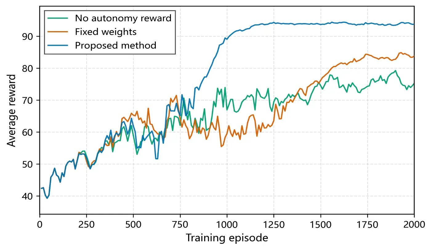
Figure 2 shows the average reward curves (10-episode moving average) of the three methods (fixed-weight, no-autonomy-reward, and the proposed method) during training. The training results of the above approaches are illustrated in Figure 2.

The following observations can be made:

Fixed-weight method (Method 1) shows improved reward after introducing a fixed autonomy weight, but the convergence is slow (stabilising after about 1400 episodes), and the final reward remains lower than that of the proposed method, because the weights cannot be adjusted dynamically according to system states.

No-autonomy-reward method (Method 2) yields the lowest reward and exhibits the largest fluctuation. Because this method completely ignores islanding preparedness, the policy tends to oscillate and has difficulty converging when conflicts arise between peak electricity prices and low SOC.

Proposed method (Method 3) enters a stable high-reward region after about 900 episodes, with significantly smaller fluctuations than the other two. This benefit stems from two aspects: first, the dynamic weighting network automatically adjusts the optimisation focus based on real-time states (SOC, autonomy index, electricity price), avoiding ineffective oscillation among objectives; second, the adaptive truncation coefficient allows larger steps for exploration in the early stage and automatically shrinks for stable fine-tuning later, effectively balancing exploration and exploitation.

To examine whether the dynamic weighting network can adaptively adjust the optimisation focus according to system states, a typical day is selected for analysis. On this day, PV output is abundant, the electricity price peaks at noon, and an islanding fault is pre-set in the evening (external grid fault at 20:00). Figure 3 presents the 24-h evolution of the economic weight $${w_{{\rm{econ}}}}$$, security weight $${w_{{\rm{safe}}}}$$, and autonomy weight $${w_{{\rm{auto}}}}$$, overlaid with the time-of-use price, the average SOC of the BESS, and the degree of autonomy for reference.The daily variation characteristics of each weight and related operational indicators are clearly depicted in Figure 3.

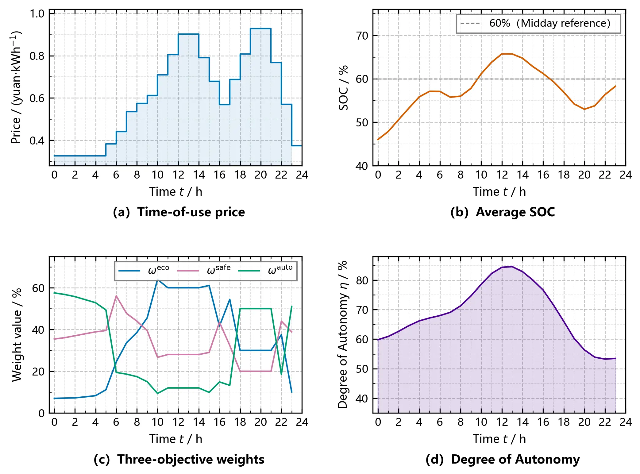
Noon period (11:00–14:00): PV output reaches its peak, and the electricity price is high, while the average SOC of the BESS remains above 0.72. The dynamic weighting network automatically raises the economic weight to about 0.55–0.60, guiding the system to increase electricity sales and reduce purchases to profit from peak-hour prices. Meanwhile, because the SOC is sufficient, the autonomy weight stays at a low level of 0.20–0.25, and the security weight remains around 0.20.

Evening period (18:00–21:00): PV output drops to zero, the load reaches its peak, and the electricity price is still high, but the average SOC of the BESS falls to about 0.58 due to daytime discharge. At this time, the autonomy index declines, and the dynamic weighting network responds quickly: the economic weight decreases to 0.35–0.40, while the autonomy weight rises to 0.45–0.50. This shift reduces BESS discharge, lowers EV charging power, and places interruptible loads on standby, thereby reserving capacity for potential islanding. The security weight also increases slightly to 0.25–0.30, strengthening the penalty for power balance deviations.

Night valley period (23:00–05:00): The electricity price is lowest. The economic weight drops to about 0.25, and the autonomy weight rebounds to above 0.50. The system purchases electricity at low prices to charge the BESS while maintaining the SOC in a healthy range of 0.60–0.70.

These results demonstrate that the dynamic weighting network can adjust the optimisation focus in real time according to state variables such as electricity price, SOC, and autonomy index, achieving an adaptive trade-off between economy and autonomy. The fixed-weight method cannot achieve such a dynamic response, as its weights remain constant throughout the day, leading to excessive conservatism at noon and excessive risk-taking in the evening.

It is worth emphasizing that the dynamic weights are not manually tuned; they emerge from end-to-end training of the lightweight network. As shown in Figure 3, the network learns to elevate the autonomy weight when the SOC approaches the lower safety threshold (20%) during peak-load hours, thereby automatically prioritizing reserve capacity over arbitrage profit—a behavior that aligns with battery-protective operational practices without requiring explicit if-then rules. This data-driven weight generation mechanism enables the proposed strategy to generalize across diverse operating scenarios without relying on heuristic weight schedules.

An external grid fault is set at time $$t = 20$$ (20:00), requiring the microgrid to operate in islanded mode for 4 h. In this scenario, the islanding preparedness and operational economy of the three methods are compared.

Two core metrics in the subsequent table are clarified in advance: the PV utilization rate refers to the ratio of the actual PV energy injected into the microgrid to the total available PV energy over the scheduling horizon; the EV regulation rate quantifies the fulfillment degree of EV charging demands, defined as the ratio of the actual delivered charging energy to the total requested charging energy of all EV chargers. The formal mathematical definitions of the two metrics are detailed in Section 4.5. Table 1 summarises the test results.

Result analysis:

Economy: The no-autonomy-reward method (Method 2) achieves the lowest daily operating cost (14,800 CNY) because it completely sacrifices islanding preparedness, selling large amounts of electricity during peak hours, and buying during valley hours. However, this strategy severely degrades islanding survivability. The fixed-weight method (Method 1) has the highest cost (18,650 CNY) because its fixed weights prevent it from fully profiting during peak prices while retaining excessive autonomy capacity during inefficient periods. The proposed method achieves a daily operating cost of 15,920 CNY, which is 14.6% lower than Method 1 and only 7.6% higher than Method 2, but it obtains a substantial improvement in islanding capability.

Islanding preparedness: The proposed method reaches an average SOC of 0.64 before islanding, which is 56% higher than Method 2 (0.41) and 36% higher than Method 1 (0.47). The critical load interruption time is only 5 min, 72% shorter than Method 1 (18 min) and 89% shorter than Method 2 (44 min). These results validate that the dynamic autonomy weight effectively guides the system to reserve islanding capacity during grid-connected operation, and the reservation cost (an extra 7.6% in operating cost) is far lower than the loss caused by islanding failure.

Security: The proposed method has zero power balance violations, whereas Method 1 has 2 violations and Method 2 has 9 violations, indicating that ignoring the autonomy objective not only impairs islanding capability but also increases security risks during normal operation.

PV utilization and demand response: The proposed method achieves a PV utilization rate of 93.3%, which is better than Method 1 (91.2%) and slightly lower than Method 2 (94.1%). The difference is acceptable. The EV regulation rate is 73.8%, lying between Method 2 (84.2%) and Method 1 (67.5%), indicating that the proposed method strikes a balance between economy and flexibility.

In summary, the dynamic autonomy weighting mechanism achieves a Pareto improvement between economy and autonomy: a small economic cost (7.6% increase over the no-autonomy-reward method) is traded for a large gain in islanding preparedness (89% reduction in interruption time), while outperforming the fixed-weight method in all metrics.

Before presenting the detailed coordination analysis, two core performance metrics from the previous experimental comparison are formally defined using standardized mathematical expressions to eliminate ambiguity: the EV regulation rate and PV utilization rate.

The EV regulation rate quantifies the fulfillment degree of electric vehicle charging demands within the scheduling horizon, which reflects the demand response capability of EV charging station agents and the guarantee level of user charging experience. Mathematically, it is defined as the ratio of the total actual charging energy delivered to EVs to the total theoretical charging energy requested by EV users over the 24-h scheduling period, with the expression as follows:

where:

$${\bm{\eta }}_{\text{EV,reg}}$$ denotes the EV regulation rate, expressed as a percentage;

$${\mathbf{N}}_{\text{EV}}$$ is the total number of independent EV chargers in the microgrid system (set to 20 in the case study);

$$\mathbf{T}$$ is the total number of dispatch intervals within the scheduling horizon ($$\mathbf{T=24}$$ for a 24-h scheduling period with 1-h resolution);

$${\mathbf{P}}_{\text{EV,n}}\left(\mathbf{t}\right)$$ is the actual charging power of the $$\mathbf{n}$$-th EV charger at time interval $$\mathbf{t}$$, unit: kW;

$$\mathbf{\Delta }\mathbf{t}$$ is the length of each dispatch interval, set to 1 h in this paper;

$${\mathbf{E}}_{\text{EV,n}}^{\text{req}}$$ is the total requested charging energy (i.e., daily charging demand) of the $$\mathbf{n}$$-th EV charger, unit: kWh.

A higher EV regulation rate indicates that a larger proportion of users’ charging demand has been satisfied, and the demand response regulation has a smaller impact on user charging experience.

The PV utilization rate is defined as the ratio of the actual PV energy injected into the microgrid to the total available PV energy over the 24-h scheduling horizon and measures the system’s renewable energy accommodation capacity. The mathematical expression is as follows:

where:

$${\bm{\eta }}_{\text{PV,util}}$$ denotes the PV utilization rate, expressed as a percentage;

$${\mathbf{N}}_{\text{PV}}$$ is the total number of independent PV arrays in the system;

$${\mathbf{P}}_{\text{PV,m}}^{\text{grid}}\left(\mathbf{t}\right)$$ is the actual grid-connected power of the $$\mathbf{m}$$-th PV array at time $$\mathbf{t}$$, unit: kW;

$${\mathbf{P}}_{\text{PV,m}}^{\text{max}}\left(\mathbf{t}\right)$$ is the forecasted maximum available power of the $$\mathbf{m}$$-th PV array at time $$\mathbf{t}$$, unit: kW.

This subsection analyses the coordinated behaviour of the 53 agents under the proposed method, focusing on the PV utilization rate, load satisfaction rate, and differentiated responses of different agent types.

PV utilization rate and load satisfaction rate: Under the proposed method, the average daily utilization rate of the ten PV units is 93.3%. PV utilization mainly occurs during the noon peak-price period (11:00–13:00) when the BESS SOC exceeds 0.85, and the economic weight is high; the system selectively curtails PV to avoid reverse power flow and voltage violations. Compared with the fixed-weight method (91.2%), the proposed method improves the utilization rate by 2.1 percentage points because the dynamic weighting network can more precisely coordinate BESS discharge and EV charging load to make room for PV integration. Compared with the no-autonomy-reward method (94.1%), the proposed method is slightly lower by 0.8 percentage points, but the latter sacrifices islanding capability. Just as shown in Figure 4:

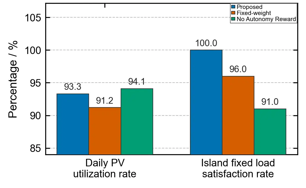
Supply reliability for fixed loads is a basic requirement for the microgrid. Before the islanding fault occurs, all three methods maintain a fixed load satisfaction rate of 100% (no active load shedding). During the islanded operation period (20:00–24:00), the proposed method, by virtue of its reserved autonomy capacity (SOC of 0.64 before islanding), ensures a continuous power supply to critical loads, maintaining a fixed load satisfaction rate of 100% with only planned switching of interruptible loads. The no-autonomy-reward method, with an SOC of only 0.41 before islanding, experiences a power shortage in the second hour of islanded operation and is forced to shed some fixed loads, reducing the fixed load satisfaction rate to 91%. The fixed-weight method, with a pre-islanding SOC of 0.47, encounters a supply gap in the third hour, lowering the fixed load satisfaction rate to 96%. The proposed method maintains a fixed load satisfaction rate of 100% during islanding, significantly outperforming the benchmark methods.

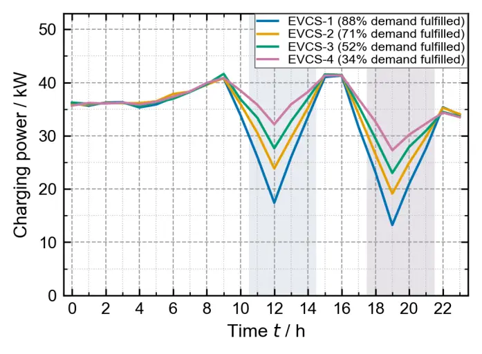
Coordination of EV charging agents: The 20 EV chargers exhibit differentiated responses on a typical day. Figure 5 shows the power curves of four representative chargers (selecting the one with the highest, medium, lowest, and an average level of daily charging demand completion). During the noon peak-price period (11:00–14:00), the average power of the chargers is reduced by about 33%. During the evening period when the autonomy weight rises (18:00–21:00), the average power is further reduced by about 48%. The reduction magnitude is negatively correlated with the daily charging demand completion rate: chargers that have already satisfied more than 80% of their daily demand show the largest reduction (up to 60%), while those with a completion rate below 40% exhibit a smaller reduction (about 25%). This demonstrates that the multi-agent architecture can achieve differentiated coordination based on each unit’s local state, rather than simple uniform control.The above charging power variation characteristics and differentiated regulation results are clearly reflected in Figure 5.

Coordination of BESS agents: The charging/discharging behaviours of the eight BESS units are highly coordinated, and their SOC trajectories tend to converge under the guidance of the centralised critic network. Figure 6 presents box-plot distributions of the SOC of all BESS units (statistics taken every 2 h). During the noon peak-price period, larger-capacity BESS units discharge slightly deeper than smaller-capacity units (as they undertake more peak-shaving arbitrage). After the autonomy weight increases in the evening, all BESS units reduce discharge and prioritise maintaining SOC levels. The SOC deviation among the BESS units remains below 5 percentage points throughout the day, indicating good coordination consistency.The statistical distribution and daily variation characteristics of BESS SOC are intuitively reflected in Figure 6.

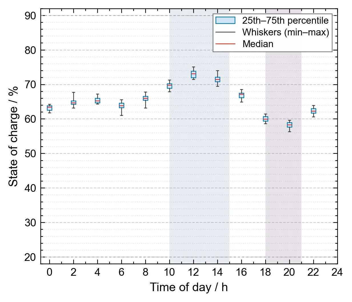
In this figure, the shaded backgrounds indicate the valley electricity price period (23:00–07:00, light gray) and the peak price periods (10:00–15:00 and 18:00–21:00, darker gray) for visual reference.

Interruptible load agents: Under the proposed method, the 15 IL groups are only briefly switched during the evening islanding transition period (20:00–21:00), with a total of 5 interruptions, a total interruption duration of 25 min, and a compensation cost of 62.5 CNY. In contrast, under the fixed-weight method, some IL groups are incorrectly switched during the noon peak-price period (because the fixed weights cannot recognise islanding risks), incurring unnecessary compensation expenditure (≈120 CNY). Under the no-autonomy-reward method, insufficient reserves during islanding force frequent switching, resulting in a total interruption duration of 95 min and a compensation cost of 237.5 CNY.

To fully validate the superiority of the proposed dynamic autonomy weight-based multi-agent coordination strategy, three mainstream advanced algorithms in the field of microgrid dispatch in recent years are added as comparative objects on the basis of the original two benchmark methods (fixed-weight method (Method 1) and no-autonomy-reward method (Method 2)). The comparative algorithms are defined as follows:

Improved SAC Algorithm: This algorithm adopts a residual-inspired network architecture to accelerate its convergence rate, with core optimization objectives targeting wind power accommodation capacity and the minimization of grid power purchase costs.

Physics-Constrained TD3 Algorithm: A differentiable safety layer is embedded in this algorithm to ensure full compliance with all system operating constraints, and it is optimized to enhance dispatch security under the non-convex constraints introduced by AC power flow calculations.

Traditional MAPPO Algorithm: The standard multi-agent proximal policy optimization (MAPPO) framework is adopted as the baseline algorithm, which does not contain the dynamic weight assignment module and adaptive clipping mechanism designed in the proposed framework.

All comparative algorithms adopt the same simulation environment, equipment parameters, and training episodes (2000 episodes) to ensure fairness. The comprehensive performance evaluation indicators include economy, autonomy, safety, renewable energy utilization efficiency, and algorithm efficiency. The detailed comparison results are presented in Table 2:

Table 2 shows that the proposed method demonstrates superior comprehensive performance across most evaluated dimensions. Economically, it achieves a daily operating cost of 15,920 CNY, which is only 7.6% higher than the purely economy-driven no-autonomy-reward method, yet delivers substantial improvements in islanding preparedness. In terms of autonomy, the proposed method attains a pre-islanding SOC of 0.64 and a critical load interruption time of only 5 min during islanding—outperforming all benchmark algorithms by significant margins, with the fixed load satisfaction rate reaching 100% without forced shedding. Safety is also ensured with zero power balance violations, benefiting from the coupled design of dynamic weights and safety rewards. Notably, these gains are achieved without compromising renewable energy utilization (PV accommodation rate of 93.3%) or algorithm efficiency (training convergence at 900 episodes, execution time of 5.5 ms/step). Collectively, these results validate the synergistic effectiveness of the dynamic weight mechanism, differentiated multi-agent modeling, and adaptive MAPPO algorithm in enabling a balanced trade-off among economy, autonomy, and safety in microgrid operation.

Aiming at the optimal operation of PV-ESS-EV hybrid microgrids, this paper develops a coordinated control strategy based on multi-agent reinforcement learning (MARL) with adaptive dynamic autonomy weights. Built on three core design components—differentiated agent modeling for heterogeneous controllable resources, a dynamic weight generation module for multi-objective optimization, and an adaptive clipped MAPPO algorithm—the proposed method effectively realizes a dynamic, adaptive trade-off among operational economy, islanding standby capacity, and grid-connected operation security. The entire strategy is constructed under the classic centralized training and decentralized execution (CTDE) paradigm, which not only guarantees excellent adaptability to diverse heterogeneous controllable resources in the microgrid, but also achieves global collaborative optimization of system operation.

In this study, islanding preparedness is defined as the microgrid’s ability to sustain critical loads during an unplanned transition to islanded mode, quantified by the energy storage’s pre-fault state of charge (SOC), the curtailable capacity of EV charging stations, and the available interruptible load margin. Under a simulated external grid fault occurring at 20:00 (peak-load period), the proposed method maintains an average SOC of 0.64 before islanding—compared to only 0.41 for the economic-only baseline—and reduces the critical load interruption duration from 44 min to just 5 min. This 89% reduction in outage time is achieved at a marginal economic cost of only 7.6% (daily operating cost increases from 14,800 CNY to 15,920 CNY). These results demonstrate that the dynamic autonomy weighting mechanism provides a quantifiable and cost-effective trade-off between economic efficiency and resilience, offering a practically viable and technically sound solution for intelligent microgrid scheduling under uncertainty.

The authors would like to thank all those who provided support and constructive feedback during the preparation of this work.

Conceptualization, Y.S.; Writing—Original Draft Preparation, Y.S.; Writing—Review, Y.X.; Supervision else, X.H., Z.W., C.W., W.W., T.Z., C.Z., W.D. and H.C.

Not applicable.

Not applicable.

The data that support the findings of this study are available from the corresponding author upon reasonable request.

This research was supported by the Sichuan Natural Science Foundation Project (2026NSFSCZY0091) and Sichuan University Student Innovation and Entrepreneur-ship Training Program (X2026106100509) and Institutional Research Fund from Sichuan University (0-1 Innovation Research Project) under Grant 2023SCUH0002.

The authors declare that they have no known competing financial interests or personal relationships that could have appeared to influence the work reported in this paper.