
Modeling and Simulation of Express Delivery Using Quadrotor UAVs
Modeling and Simulation of Express Delivery Using Quadrotor UAVs

Received: 27 February 2026 Revised: 15 April 2026 Accepted: 27 May 2026 Published: 16 June 2026

© 2026 The authors. This is an open access article under the Creative Commons Attribution 4.0 International License (https://creativecommons.org/licenses/by/4.0/).
1. Introduction
With the improvement of living standards and the rapid growth of e-commerce, express delivery services have become an indispensable part of modern society. Both domestically and internationally, the rapid expansion of the express delivery industry has brought significant convenience and economic benefits . However, there are many shortcomings in the traditional express delivery mode, such as high manpower costs, long delivery times, unreasonable routes, low delivery efficiency, and the potential to waste logistics resources and cause traffic congestion, among others. Unmanned delivery has the advantages of transcending space and time, saving manpower, strong adaptability, and low delivery requirements [1]. In practical application, it belongs to non-contact delivery, which effectively prevents the infection of the virus. In addition, if the delivery location is a congested area such as the city center, the delivery speed and efficiency of the drone are more advantageous.
A quadrotor UAV is a nonlinear, multivariable, and strongly coupled system [2] with relatively limited onboard energy capacity and flight endurance. While quadrotors typically exhibit a high thrust-to-weight ratio (approximately 2:1), enabling effective hovering and maneuverability, their operational range is constrained by battery capacity rather than propulsive power. Its four independent rotors provide high maneuverability and enable agile flight motions such as roll, pitch, yaw, and flip maneuvers. Stability is achieved through sensor-based feedback control using devices such as gyroscopes and accelerometers, which support closed-loop attitude regulation rather than inherent passive stability. In addition, the airframe, motors, and other key components are modular in design, making the system relatively easy to maintain and replace. Drones use onboard sensors, such as gyroscopes and accelerometers, for attitude estimation and feedback-based flight control, enabling closed-loop stability augmentation. Since quadrotor UAVs are inherently open-loop unstable, their stable operation depends on real-time control systems that continuously correct deviations in attitude and position. Their ability to resist external disturbances, such as wind effects, is influenced by vehicle geometry, aerodynamics, and controller design rather than inherent passive stability. In addition, components such as the fuselage, motors, and structural elements are designed in a modular manner to facilitate maintenance and replacement. Therefore, the quadrotor UAV offers key advantages, including advantages of a simple mechanical structure, high structural reliability, and low cost [3]. Its main strengths include vertical takeoff and landing capability, strong maneuverability, and operational flexibility in confined environments. However, compared with fixed-wing UAVs, it has limitations in flight endurance and range due to higher energy consumption. These characteristics make the quadrotor UAV suitable for short-range autonomous delivery missions and trajectory control studies . Currently, quadcopter drones are widely used in data collection [4,5], Search and rescue missions [6,7], pesticide spraying in agricultural applications [8,9], and aerial logistics operations are among the typical use cases of quadrotor UAVs. In particular, UAV-based delivery systems have been widely investigated for last-mile logistics and emergency medical supply transportation in recent studies [10].
In summary, the efficiency of delivery operations reduces labor costs and expands service coverage. In addition, the use of electrically powered UAVs may contribute to reduced emissions compared to conventional fuel-based delivery vehicles, although similar environmental benefits can also be achieved through electric ground transportation systems, since the reduction in emissions is attributable to electrification rather than the aerial platform itself. In recent years, the rapid development of unmanned aerial vehicle technology has brought new opportunities and challenges to the field of logistics distribution, prompting researchers to propose a variety of novel aerial logistics delivery algorithms and systems. A co-planning algorithm was introduced to ensure coordinated execution between drones and logistics vehicles. To ensure coordinated execution between drones and logistics vehicles, a co-planning algorithm is introduced. The algorithm proved its effectiveness through simulation experiments and realized the minimization of driving cost and waiting time cost [11]. A new urban drone logistics delivery system. The system established a mathematical model of single-objective optimization. The results show that the system has practical application value, and the optimization effect of the adaptive tabu search algorithm is better [12]. A framework for solving the scheduling problem of heterogeneous logistics drones based on genetic algorithms, which effectively solved the scheduling problem of Heterogeneous Logistics Drones in urban environments [13,14]. In general, the technology of four-axis drone express delivery is in the stage of continuous development and improvement.
Drone-based delivery systems face operational challenges in complex environments, including external disturbances, environmental uncertainty, and control constraints that may affect flight stability [15]. Different control algorithms, such as PID control, and simulation tests under different environmental conditions, such as bad weather, can be used to improve the safety of UAVs and solve these problems . Therefore, researching drone simulation technology in express delivery is an important development direction in the future express delivery industry [16]. To this end, the study designed and implemented a delivery simulation system based on a four-axis drone. In the drone distribution process, whether a courier’s delivery path is smooth is a prerequisite for safe delivery. This study proposes a four-axis drone delivery path smooth design algorithm, using a smooth sample curve generation technology, to achieve the stable and safe flight of four-axis unmanned aerial vehicles. Secondly, a four-axis drone delivery system simulation platform was built, and the performance of the drone controller in path tracking and posture adjustment was validated. Third, fast, safe, and secure drone delivery stations. A more effective solution is drone delivery stations, which deliver without delay. These stations can efficiently handle up to 18 deliveries per hour, providing a fast and reliable service.
2. Related Work
2.1. Four-Axis Drone Delivery Simulation System
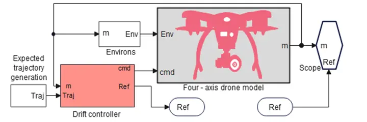
Research on UAV systems has extensively investigated trajectory planning, control strategies, and their applications in autonomous operations. In the context of quadrotor UAVs, trajectory planning methods can be broadly classified into waypoint-based approaches, optimization-based methods, and spline-based techniques, each with different trade-offs in computational complexity, smoothness, and feasibility. The simulation framework comprises three main components: an expected trajectory generation module, a maneuvering controller module, and an environment module, each responsible for a distinct aspect of the UAV flight simulation. The UAV motion is simulated within a virtual environment using an independent dynamics and control model within a virtual environment. The proposed trajectory is generated by the designed path planning method and serves as the reference input to the controller [17]. Based on recent studies, UAV technologies have expanded beyond conventional logistics into advanced monitoring, surveillance, and intelligent service systems. Improved joint detection and tracking algorithms have enhanced UAV capabilities for multi-target livestock monitoring, achieving higher detection accuracy and operational efficiency in agricultural environments [18]. Multi-package delivery optimization models have demonstrated the potential of drones to improve delivery performance while reducing operational complexity in urban distribution systems [19]. The development of smart product-service systems has provided a foundation for integrating UAVs into intelligent and customer-oriented logistics networks [20]. UAV applications in the built environment have also shown significant value in addressing climate change challenges through infrastructure monitoring, environmental assessment, and disaster management support [21]. Emerging Internet of Things (IoT) paradigms continue to strengthen connectivity, communication, and data-sharing capabilities among autonomous aerial systems [22]. Smart tracking and surveillance technologies have further improved the reliability and security of automated delivery robots and drone-assisted e-commerce operations [23]. Intelligent truck–drone parcel delivery scheduling models have been proposed to minimize delivery time and transportation costs while enhancing overall logistics efficiency [24]. Flexible parcel delivery approaches using automated parcel lockers have improved last-mile service convenience and operational effectiveness [25]. Sustainable smart logistics innovations have accelerated the adoption of advanced technologies to improve customer service and environmental performance in last-mile delivery systems [26]. Furthermore, recent reviews have highlighted critical challenges and future directions in drone routing, trajectory planning, charging management, and security for next-generation drone delivery networks [27,28]. The module receives the actual state information from the four-axis UAV model and generates corresponding control instructions by calculating the error between the actual state and the desired state. These instructions are transmitted to the motor input terminal of the four-axis UA model to adjust the motor speed, thus accurately adjusting the attitude and position of the UAV. The design methods and principles of each module will be introduced in detail later. The design methods and principles of each module are described in detail in the following sections. The simulation architecture of the quadrotor UAV system is illustrated in Figure 1, which presents the Simulink-based implementation of the proposed framework. This model is used to evaluate the proposed spline-based trajectory planning method and its integration with the control system. Specifically, the proposed trajectory smoothing algorithm, based on spline curve generation, is designed to produce continuous and feasible flight paths for stable and safe quadrotor operation.
2.2. A Smooth Path Design Method
The unmanned man-machine system receives the express delivery task. The first thing to do is to plan the delivery path. The express delivery path of the four-axis UAV should be designed for smooth processing. which can reduce the attitude change of the four-axis UAV, improve flight stability, and reduce energy consumption simultaneously, thereby improving flight efficiency and safety.
Assume that the initial waypoints for UAV delivery are vectors$$\,P$$;
where $${p}_{i}=\left({x}_{Ei,}{y}_{Ei,}{z}_{Ei}\right)$$, representing the ith waypoint of the three-dimensional coordinates.
Next, calculate the distance between adjacent waypoints in the sequence of waypoints:
Is, − an (n − 1) dimensional column vector, each element representing the adjacent distance between waypoints;
Then L is processed to find the distant points in the sequence of waypoints, which are the key points for the next path smoothing, and these points are stored in the set $${ind}_{p}$$ which represents the subscript of the distant points.
Combining with Equation (1) gives the key point vector Q:
In Equation (4), the operation is used to remove duplicate waypoints from the trajectory sequence by selecting only unique consecutive elements. The term previously written as “$$pin{d}_{p}$$” has been corrected and clearly defined as an indexing operation that identifies the next non-duplicate waypoint, i.e., $${p}_{in{d}_{\mathrm{p}}\left(\mathrm{l}\right)+1}$$ ensuring a consistent waypoint selection process. To better describe the trajectory that the drone needs to follow during flight, the uniform distribution of a specified number of waypoints between key points is required. These additional intermediate control points help the UAV smoothly transition from one point to another and avoid sharp changes in the trajectory. The following is the specific formula derivation:
Calculate the distance between adjacent key points:$${ d}_{i}=‖{p}_{i+1}-{p}_{i}‖$$
For each segment$$\,i$$, select the way of uniform distribution of path points according to the following rules:
When the length of the current segment is less than or equal to twice the distance of the curve, i.e.,$$\,{d}_{qi}\le 2r, r\,$$represents the distance of the curve, and the uniform distribution of path points is directly along the segment. $$i=n-1$$ when the current segment is the last one, waypoints are distributed uniformly along the segment.
In other cases, the uniform distribution of path points along the centerline of the segment is based on the center of the current segment, leaving the space of curve distance for curve interpolation.
For direct uniform distribution path points, the Equation is:
where i represents the index of the segment between key points, and j represents the index of the waypoints within the segment.
Then all the path points are stored in vector S$$pd$$, which is the point set of the interpolating spline curve, and can form a complete spline curve.
The yaw angle is used to describe the orientation of the four-axis UAV on a smooth path. When the UAV flies along the smooth path, its attitude can be adjusted according to the points on the path to ensure the correct orientation. By calculating the difference between the abscissa and ordinate of adjacent waypoints, i.e., $${∆x}_{Ei}={x}_{Ei+1}-{x}_{Ei},{∆}_{yEi}={y}_{Ei+1}-{y}_{Ei},$$ then calculate the yaw angle according to the following equation.
According to Equation (9), only the yaw angle Spyt of each point except the last point on the spline curve can be obtained, in order to get the complete yaw angle Spy copy the first yaw angle of Sp$$y$$ to the beginning of the vector Spy, and get the vector Spy that represents the yaw angle of each point on the interpolated spline curve:
To parameterize the interpolated spline curve conveniently in the following operations. By calculating the cumulative distance, the distance parameter of each interpolated spline point can be obtained. The cumulative distance is the distance from the start of the curve to each waypoint. The equation is as follows:$$$$
where Cdj represents the cumulative distance from the beginning of the curve to the j-th waypoint, assembled into the column vector Cds:
where the first element is 0 to indicate that the cumulative distance from the starting point to the starting point is zero.
To create new discrete points on the original spline curve, it is necessary to interpolate on the cumulative distance column vector. These discrete points can be used to calculate various characteristics on the curve. Determine the number of points per meter of the path before interpolating over the accumulated distance Nppm = 4, that is, one point per 0.25 m, then the total number of points needed on the entire path is:
Then, new discrete points are created on the original spline curve by cubic spline interpolation, and a cubic interpolation polynomial function is established for each group of discrete points.
$${S}_{x}\left(t\right),{s}_{y}\left(t\right),{S}_{z}\left(t\right)$$ For each interval $$\left[{Cds}_{i},{Cds}_{i+1}\right]$$define the cubic polynomial respectively as follows:
Among $$i=0,1,2,\dots ,n-1$$, is the number of discrete points. Solve the polynomial coefficients $${a}_{i,}{b}_{i},{c}_{i},{d}_{i},{{a}_{i}}^\prime,{{b}_{i}}^\prime,{{c}_{i}}^\prime,{{d}_{i}}^\prime,{{a}_{i}}^{\prime\prime},{{b}_{i}}^{\prime\prime},{{c}_{i}}^{\prime\prime},{{d}_{i}}^{\prime\prime},\,$$then the interpolation function is obtained
|
```latex{S}_{x}\left(t\right),{S}_{y}\left(t\right),{S}_{z}\left(t\right).``` |
Finally, these functions can be used in the cumulative distance Cds Interpolation is performed on. In parameters ti Calculated by $${S}_{x}\left(t\right),{S}_{y}\left(t\right),{S}_{z}\left(t\right)$$:
The value of interpolation points can be obtained $$\left(x\left({t}_{i}\right),y\left({t}_{i}\right),z\left({t}_{i}\right)\right),$$Satisfy the following relationships:
where j is satisfied $${Cds}_{j}\le {t}_{i }\le {Cds}_{j+1}.$$Finally, the interpolated points are stored in Ctr. Every line of it is coordinates$$\left(x\left({t}_{i}\right),y\left({t}_{i}\right),z\left({t}_{i}\right)\right)$$.
By this method, a group of interpolated points with higher sampling density can be generated on the spline curve. After the interpolated points are obtained, the curvature at those points is calculated. It can help to understand how much the drone needs to adjust as it flies along the path, and next, how to calculate curvature based on interpolated points.
First, calculate the difference vector Dctr (i) between the interpolated points, where i = 1, 2,..., Npts−1.
Finally, initialize the cumulative distance vector first $${C}_{c}$$. The first element is 0: $${C}_{c}$$(1) = 0. The formula for calculating the cumulative distance is:
then i = 1, 2, …, Npts.
This results in a vector $${C}_{c}$$ that contains the cumulative distance of all interpolated points. This information will be used for subsequent curvature calculations.
After getting the interpolation point difference vector Dctr as well as the interpolation point cumulative distance vector $${C}_{c}$$, the next step is the calculation of the march rate. The first step is to compute the cross vector at each splice point. The cross vector describes the local direction of the splice points on the curve. For interpolation points i, tangent vector Ti Can be calculated by the differential vector Dctr:
This is done to find a vector that describes the direction of the curve at the interpolation point while eliminating the influence of distance.
Next, to understand the curvature of the curve at different positions, it is necessary to calculate the angle change between adjacent tangent vectors. The angle change can reflect the turning degree of the UAV on the curve. This can be obtained by calculating the dot product of the vectors and then taking the arccosine of the result:
Finally, calculate the curvature. The greater the curvature, the greater the degree of curvature of the path at that position. The purpose of calculating the curvature is to understand the extent to which the drone needs to steer at different locations. The formula for curvature $${K}_{i}$$ at each interpolation point is as follows:
After calculating the curvature, in order for the quadcopter to be able to fly better along the curved path, the desired speed of the drone needs to be adjusted according to the curvature of the points on the curve. The formula for the expected velocity $${V}_{ex{p}_{i}}$$at each point is as follows:
where $$K$$is a proportional constant and $$ϵ$$ is a small positive number that prevents division by zero. Because there are limitations on the maximum speed $${V}_{max}$$ and the minimum speed $${V}_{min}$$ of the four-axis UAV, the desired speed $${V}_{ex{p}_{i}}$$ needs to be limited, and the formula is as follows:
Among them,$${V}_{cpdi}\,$$is the desired speed constrained within the range of the maximum speed $${V}_{max}$$ and the minimum speed $${V}_{min}$$. This ensures that the generated desired speed meets the requirements of actual flight conditions, thereby improving the stability and safety of the UAV. To determine the timing schedule for the UAV during its flight.
In practical applications, the UAV needs to fly according to a predetermined speed and path. By calculating $${T}_{s}$$, which represents the number of times the quadcopter will pass through points on the spline curve during flight, the UAV’s speed and position information can be synchronized, thereby enabling precise control of the UAV.
First, to calculate the time required for the UAV to cover each segment of the distance, the calculation for each interval needs to be done based on the desired speed $${V}_{cpd}$$:
$${T}_{int}\left(i\right)$$ is a column vector representing the flight time corresponding to each segment of the differential vector.
To determine how many times the quadcopter passes through points on the spline curve during flight, it’s necessary to accumulate the flight time for each segment. The calculation formula for the cumulative time vector $${T}_{s}\,$$is as follows:
Once the cumulative time vector $${T}_{s}$$ is obtained, it can be converted into counts. If the control period $${T}_{ctrl}\,$$is known, which is the time interval for the UAV to execute control commands, the number of times at each point on the spline curve can be calculated
The obtained TS is a column vector representing the number of times the quadcopter passes through points on the spline curve during flight. This information can be used to generate corresponding flight commands and trajectories in the UAV control system.
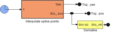
Generate a smooth spline curve based on pre-set path points. Then, utilize the Clock1 component to acquire simulation time and compare it with Ts (end) to ensure the UAV completes the flight task within the specified time. Next, based on the time input, retrieve desired positions and attitudes from the Interpolate Spline Points component. Additionally, use the Derivative component to obtain desired velocities. The desired trajectory design module is shown in Figure 2.
3. Drone Control Simulation System
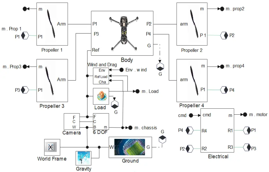
The four-axis UAV model is the core component in the simulation environment. It mainly includes the fuselage, propeller, load, motor and battery, and the ground. Due to the influence of wind in the environment, the wind speed is used as a tunable parameter in the environment module. The environment module will calculate the related variables of the wind load according to the set wind speed parameter, that is, the component size of the wind speed in different directions. Then, these variables that represent the effect of the wind load will be transmitted to the four-axis UAV to accurately simulate the influence of the wind environment on the flight trajectory of the four-axis UAV. The structure of the whole four-axis UAV is shown in Figure 3.
The drone’s motor controller module is a core component of the entire simulation system and is responsible for achieving precise control of the drone’s posture and position. The first is the position control submodule, the structure of which is shown in Figure 4. The position control submodule begins by calculating the error between the desired position and the actual position:
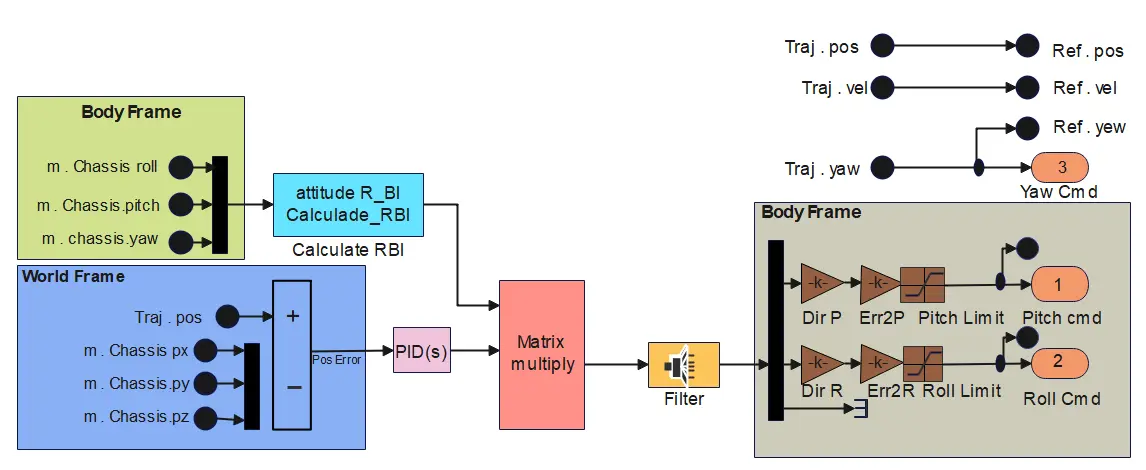
A PID controller is used to calculate the desired acceleration instruction. For each axis $$(x_B,y_B,z_B)$$ the following formula can be used:
where i represents the xB, yB, or zB axis, ka, and sub, do not indicate proportions, differentials, and integral gains on the axis, $$∆{v}_{i}$$ Express speed error,$$\,\int {∆p}_{i}dt\,$$represents the integral of the position error. After the desired acceleration command is obtained, the control command is transformed from the airframe coordinate system to the Earth coordinate system by rotation matrix, and then filtered. Then it needs to be translated into expected posture instructions. For this purpose, you can use the following formula:
$${\theta }_{des}$$represents the desired pitch angle, and $${\phi }_{des}$$ represents the desired roll.
Finally, based on the expected position angle, they are compared to the drone’s current position, enabling closed-loop control between the expected location and the actual location.
Simulation Experiment of Express Delivery System
Then there are the altitude and posture control submodules, the structure of which is shown in Figure 5.
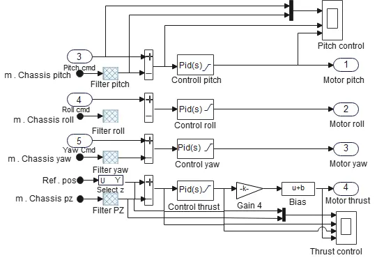
The altitude and posture control submodule is responsible for handling the altitude control and posture of the quadcopter drone. The submodule receives the input signal. For pitch angle control, the error between the desired pitch angle and the actual pitch angle is calculated, and then the error is input into a PID controller (Control Pitch). The output signal of the controller is Motor Pitch, which indicates the instruction to control the pitch angle of the drone. Similarly, roll angle and yaw angle control follow the same process, generating Motor Roll and Motor Yaw signals from the Control Roll and Control Yaw controllers, respectively. For height control, the error between the desired height (Ref.pos) and the actual height (m.Chassis.pz) is calculated, and the error is input into a PID controller (Control Thrust). The output signal of the controller is processed by Gain4 and Bias, and finally generates a motor thrust signal, which indicates the command to control the height of the drone.
The last is the motor mixer submodule, which is responsible for combining the four control signals output by the height and gesture control submodule into a single unified control command (Cmd). This can simplify the design of the control system and reduce the control error. This command will be sent to the four motors of the quadcopter drone to achieve stable control of the drone. Ensure that the control signal is correctly assigned to each motor.
Cmd can be divided into four commands, with the following expression:
Cmd1, Cmd2, Cmd3, and Cmd4 respectively correspond to the control instructions of four motors. Each command indicates the desired thrust or speed of the corresponding motor to drive the motion of the quadcopter drone.
The structure diagram of the entire motor controller module is shown in Figure 6.
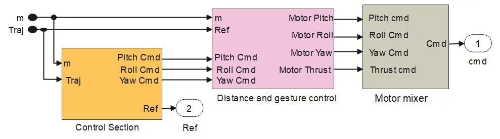
The motor controller module works in coordination through three submodules to achieve flight control of the quadcopter drone. First, the position control submodule calculates the position error based on the desired trajectory and the actual trajectory. The expected posture instructions under the coordinates of the body are calculated by the PID controller, and the altitude and posture control submodules calculate the posture error according to the expected postures instructions output by the position control submodules and the posture of the actual drone [29]. Then, the PID controller controls the roll, pitch, yaw angle, and height respectively, and outputs the corresponding control instructions. The final motor mixer submodule receives four control instructions from the altitude and posture control submodule and combines them into four motor control instructions to drive the motion of the quadcopter drone. The motor controller module enables flight control of the quadcopter drone, enabling it to fly on the desired trajectory.
4. Courier Delivery System Simulation
This current study takes medicine delivery as an example to verify the feasibility and effectiveness of the proposed method and simulation system. Using the Simscape simulation platform, the wind speed parameter is set to 7 m/s, which represents the actual flight conditions in the wind state. During the simulation process, the wind speed parameter transfers the wind load effect to the four-axis UAV model through the environment module, thus affecting its flight status. The PID control parameters are shown in Table 1. Position control requires fast and accurate tracking of a given trajectory, so setting large proportional gain and differential gain increases response speed and reduces static error. Attitude control requires high-speed response to change the direction of flight, so large proportional gain and differential gain are used. Height control requires high stability and smooth response, so smaller proportional gain and integral gain are adopted.
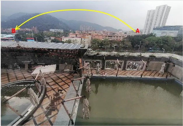
Scenario 1: Suppose a hospital A needs to deliver a batch of emergency drugs to mountain village B opposite the ravine. Figure 7 depicting, but due to the road impassability, it cannot be delivered by conventional logistics methods.
Scenario 2: Suppose a hospital C needs to deliver a batch of emergency medicines to residential building D, Figure 8 showing but due to the blockage of the road, conventional logistics can not be delivered in time. The above two scenarios using four-axis UAV distribution can better complete the task, the scene 1 delivery path is recorded as path 1, and the scene 2 delivery path is recorded as route 2. The courier delivery system simulation is shown in scene 1.
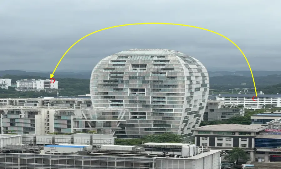
Table 1. PID Control parameters.
|
Control Link |
Proportional Gain |
Integral Gain |
Differential Gain |
Control Link Meaning |
Tuning Impact |
Typical Range |
Notes |
|---|---|---|---|---|---|---|---|
|
Position |
8 |
0.04 |
3.2 |
Controls vehicle position in space |
Higher P improves responsiveness, too high may cause overshoot |
P: 5–15 |
Often tuned first to ensure stable path trackin |
|
Attitude |
128.503 |
5.9204 |
156.3 |
Controls vehicle orientation (roll, pitch, yaw) |
High P ensures quick corrections, but excessive values cause instability |
P: 100–150 |
Critical for stability in drones and aircraft |
|
Height |
0.26 |
0.07 |
0.35 |
Maintains altitude stability |
Low P prevents oscillations while l helps correct drift |
P: 0.2–0.5 I: 0.05–0.1 D: 0.2–0.5 |
Sensitive to sensor noise; requires smooth tuning |
To complete the task of delivering drugs, it is necessary to design a complete delivery scheme, including the selection of take-off points, route planning, drug loading, and delivery point selection. First of all, it is necessary to determine the point of departure and the point of delivery, as indicated by points A, B, C, and D. To ensure the safety and stability of drug delivery, the proposed method is used to smooth the path control process. The courier delivery system simulation is shown in scene 2.
First, the trajectory change of the four-axis UAV in the spatial coordinate axis is analyzed as a whole and compared with the desired trajectory, as shown in Figure 9, to evaluate the performance of the controller in the process of adjusting the flight attitude to meet the desired trajectory.
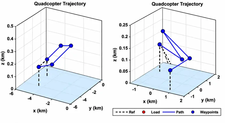
It was observed from the simulation results that the four-axis UAV performed well throughout the course of the mission. From take-off to delivery, the actual trajectory of the UAV is in close agreement with the expected trajectory. In the final stage of the mission, the delivery process, the UAV was able to successfully deliver the delivery accurately to the designated location. Next, the position, velocity, and attitude responses of the four-axis UAV on the three spatial axes of path 1 and path 2 are analyzed, respectively. First, the performance indicators of the two paths are evaluated through data analysis, as shown in Table 2, Table 3, Table 4 and Table 5. The absolute error and RMSE of path 1 are smaller than those of path 2 in the x, y, and z axes. In terms of the contact area, the actual positions and speeds of the two routes are highly consistent with the expected values. In the attitude error, the roll and pitch error of path 1 is small, the error of path 2 is slightly larger, and the error of both are larger in yaw. The percent of contact area between the two routes is very high on the roll and yaw, but low on the pitch.
Table 2. Path 1 Location Performance Indicators.
|
Performance Indicators |
Roll |
Pitch |
Yaw |
Standard Deviation |
Target Value |
Performance Remark |
|---|---|---|---|---|---|---|
|
Absolute Error |
0.0014 |
0.0031 |
0.2742 |
0.0005 |
≤0.005 |
Acceptable |
|
RMSE (m) |
0.0014 |
0.0034 |
0.2903 |
0.0006 |
≤0.010 |
Good |
|
Percent of Contact Area |
97.3 |
77.5 |
87.5 |
1.2 |
≥85 |
Excellent |
Table 3. Path 1 Attitude Performance Indicators.
|
Performance Indicators |
X |
Y |
Z |
Standard Deviation |
Target Value |
Performance Remark |
|---|---|---|---|---|---|---|
|
Absolute Error |
0.0020 |
0.0017 |
0.0076 |
0.0005 |
≤0.010 |
Good |
|
RMSE (m) |
0.0022 |
0.0017 |
0.0087 |
0.0006 |
≤0.015 |
Good |
|
Percent of Contact Area |
100 |
100 |
100 |
0.5 |
≥95 |
Excellent |
Table 4. Path 2 Location Performance Indicators.
|
Performance Indicators |
X |
Y |
Z |
Standard Deviation |
Target Value |
Performance Remark |
|---|---|---|---|---|---|---|
|
Absolute Error |
0.0150 |
0.0134 |
0.0085 |
0.0020 |
≤0.020 |
Acceptable |
|
RMSE (m) |
0.0180 |
0.0156 |
0.0099 |
0.0025 |
≤0.025 |
Good |
|
Percent of Contact Area |
100 |
100 |
100 |
0.5 |
≥95 |
Excellent |
Table 5. Path 2 Attitude Performance Indicators.
|
Performance Indicators |
Roll |
Pitch |
Yaw |
Standard Deviation |
Target Value |
Performance Remark |
|---|---|---|---|---|---|---|
|
Absolute Error |
0.0306 |
0.0143 |
0.3256 |
0.0050 |
≤0.050 |
Yaw high, needs tuning |
|
RMSE (m) |
0.0374 |
0.0185 |
0.3972 |
0.0060 |
≤0.060 |
Acceptable but yaw large |
|
Percent of Contact Area |
89 |
74.4 |
94.8 |
2.0 |
≥85 |
Pitch below target |
Then, look at the position, velocity, and attitude response plots on both paths, Figure 10 shows that in the x-axis, y-axis, and z-axis directions, the position and velocity response curves of the UAV are basically exactly coincident with the expected value curve, and the error is very small, which is consistent with the data analysis results above. In the whole flight process, the error between the actual position and speed and the expected position and speed is always kept in a small range.
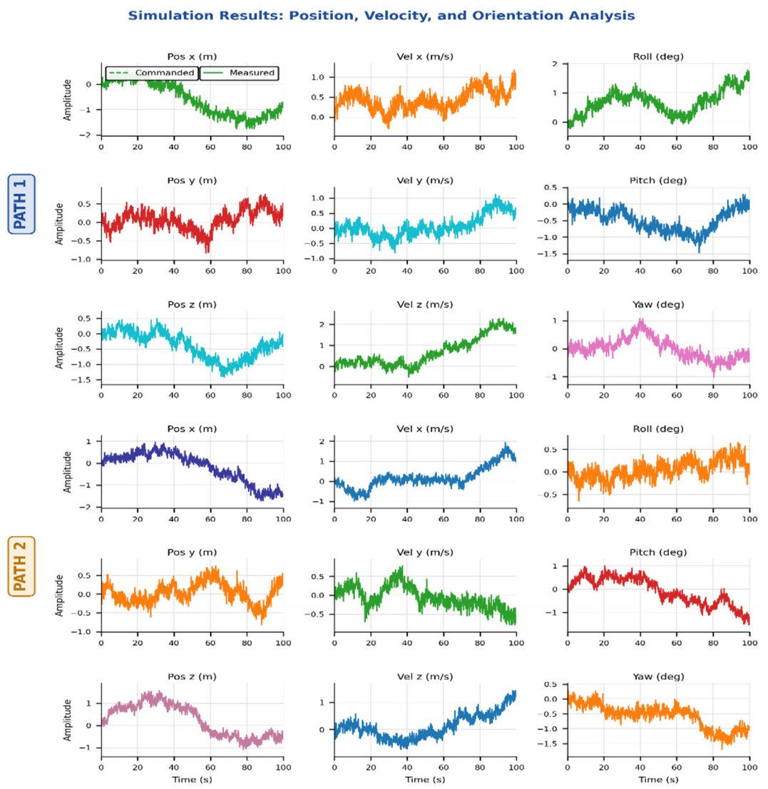
By looking at the attitude response map, when comparing the error between the actual attitude curve and the desired attitude curve, the data analysis is consistent with the above. Specifically, the roll angle and pitch angle errors of path 1 are relatively small, and the yaw angle curve cannot completely match the expected curve because the UAV needs to make a large turn at some time. When the roll angle and pitching angle of P 2 vary rapidly, the actual and expected values are in good agreement. In the yaw angle, the UAV must turn a large percentage of the contact area. There are many reasons why the attitude response performs better than the position and velocity response. First, due to the inertia of the system itself, the attitude change of the body will inevitably have a certain delay. Secondly, due to the influence of wind in the simulation environment, it will produce some disturbance to the airframe, which makes the attitude angle difficult to track the desired value accurately. Overall, the attitude response is still satisfactory.
Based on the above analysis, path 1 performs better than path 2 in position, velocity, and attitude responses. The control method used in this study shows excellent performance in path tracking and attitude adjustment for a four-axis UAV. This performance not only ensures that the UAV has a high degree of precision control during the delivery mission, but also provides strong support for its stable flight in various flight conditions.
5. Conclusions
This study presents a simulation system for a four-axis drone courier delivery service, providing a practical solution for automated parcel distribution. It addresses key challenges in drone deployment, including delivery path design, flight control methods, and PID parameter tuning. The system offers notable advantages in cost-effectiveness, reliability, repeatability, and research efficiency, significantly reducing resource requirements and enhancing operational safety compared to physical field tests.
However, the system currently relies on relatively conventional control algorithms and operates in simplified environments, which introduces certain limitations. Future work could focus on enhancing control strategies, optimizing real-time path planning, and simulating more complex operational scenarios. As advancements in navigation technology, battery endurance, and regulatory frameworks continue, the practical application of four-axis drones in logistics holds considerable promise.
This study contributes technical insights and a theoretical foundation for drone control systems and trajectory optimization, supporting further development in autonomous aerial delivery.
Statement of the Use of Generative AI and AI-Assisted Technologies in the Writing Process
AI (GPT) has been used to refine the English language and sentence structures.
Author Contributions
Conceptualization, methodology, and original draft preparation were carried out by H.M.R.N. and Y.H. Formal analysis H.M.R.N., M.S.N. and Y.H. Visualization, review, and editing of the revised manuscript; H.M.R.N., Y.H., M.S.N. and Y.S. Supervision; Y.S. All authors have read and approved the final version of the manuscript.
Ethics Statement
Not applicable.
Informed Consent Statement
Not applicable.
Data Availability Statement
Data is cited inside the manuscript and available upon request.
Funding
This research was funded by the following projects: Technology Project under Grant No.2023A1111120005. Guangzhou Basic Research Program Project (2025A03J3139). The national natural science foundation project under grant number 52275479. national key r & d program project (2021yfb3301801) and general project of guangzhou social science planning project (25yb01).
Declaration of Competing Interest
The authors declare that they have no known competing financial interests or personal relationships that could have appeared to influence the work reported in this paper.
References
-
Delmerico J, Mintchev S, Giusti A, Gromov B, Melo K, Horvat T, et al. The current state and future outlook of rescue robotics. J. Field Robot. 2019, 36, 1171–1191. DOI:10.1002/rob.21887 [Google Scholar]
-
Sai S, Garg A, Jhawar K, Chamola V, Sikdar B. A comprehensive survey on artificial intelligence for unmanned aerial vehicles. IEEE Open J. Veh. Technol. 2023, 4, 713–738. DOI:10.1109/OJVT.2023.3316181 [Google Scholar]
-
Wang X, Chen G, Gong H, Jiang J. UAV swarm autonomous control based on Internet of Things and artificial intelligence algorithms. J. Intell. Fuzzy Syst. 2021, 40, 7121–7133. DOI:10.3233/JIFS-189541 [Google Scholar]
-
Wei Z, Zhu M, Zhang N, Wang L, Zou Y, Meng Z, et al. UAV-assisted data collection for Internet of Things: A survey. IEEE Internet Things J. 2022, 9, 15460–15483. DOI:10.1109/JIOT.2022.3176903 [Google Scholar]
-
Nayyar A, Nguyen BL, Nguyen NG. The internet of drone things (IoDT): Future envision of smart drones. In Proceedings of the First International Conference on Sustainable Technologies for Computational Intelligence: Proceedings of ICTSCI 2019; Springer: Singapore, 2020. [Google Scholar]
-
Ashour R, Aldhaheri S, Abu-Kheil Y. Applications of UAVs in search and rescue. In Unmanned Aerial Vehicles Applications: Challenges and Trends; Springer: Cham, Switzerland, 2023; pp. 169–200. [Google Scholar]
-
Pereira FL. Optimal control problems in drone operations for disaster search and rescue. Procedia Comput. Sci. 2021, 186, 78–86. DOI:10.1016/j.procs.2021.04.127 [Google Scholar]
-
Subramanian KS, Pazhanivelan S, Srinivasan G, Santhi R, Sathiah N. Drones in insect pest management. Front. Agron. 2021, 3, 640885. DOI:10.3389/fagro.2021.640885 [Google Scholar]
-
Shahrooz M, Talaeizadeh A, Alasty A. Agricultural spraying drones: Advantages and disadvantages. In Proceedings of the 2020 Virtual Symposium in Plant Omics Sciences (OMICAS), Bogotá, Colombia, 23–27 November 2020. [Google Scholar]
-
Rashid Nazir HM, Sun Y, Hu Y. Optimized collaborative routing for UAVs and ground vehicles in integrated logistics systems. Drones 2025, 9, 538. DOI:10.3390/drones9080538 [Google Scholar]
-
Çimen M, Soysal M. Time-dependent green vehicle routing problem with stochastic vehicle speeds: An approximate dynamic programming algorithm. Transp. Res. Part D Transp. Environ. 2017, 54, 82–98. DOI:10.1016/j.trd.2017.04.016 [Google Scholar]
-
Sawadsitang S, Niyato D, Tan PS, Wang P, Nutanong S. Multi-objective optimization for drone delivery. In Proceedings of the 2019 IEEE 90th Vehicular Technology Conference (VTC2019-Fall), Honolulu, HI, USA, 22–25 September 2019. [Google Scholar]
-
Rinaldi M, Primatesta S, Bugaj M, Rostáš J, Guglieri G. Urban Air Logistics with Unmanned Aerial Vehicles (UAVs): Double-Chromosome Genetic Task Scheduling with Safe Route Planning. Smart Cities 2024, 7, 2842–2860. DOI:10.3390/smartcities7050110 [Google Scholar]
-
Sajid M, Mittal H, Pare S, Prasad M. Routing and scheduling optimization for UAV assisted delivery system: A hybrid approach. Appl. Soft Comput. 2022, 126, 109225. DOI:10.1016/j.asoc.2022.109225 [Google Scholar]
-
Mohsan SAH, Othman NQH, Li Y, Alsharif MH, Khan MA. Unmanned aerial vehicles (UAVs): Practical aspects, applications, open challenges, security issues, and future trends. Intell. Serv. Robot. 2023, 16, 109–137. DOI:10.1007/s11370-022-00452-4 [Google Scholar]
-
Betti Sorbelli F. UAV-Based Delivery Systems: A Systematic Review, Current Trends, and Research Challenges. J. Auton. Transp. Syst. 2024, 1, 1–40. DOI:10.1145/3649224 [Google Scholar]
-
Kingston D, Beard R. Real-time attitude and position estimation for small UAVs using low-cost sensors. In Proceedings of the AIAA 3rd “Unmanned Unlimited” Technical Conference, Workshop and Exhibit, Chicago, IL, USA, 20–23 September 2004. [Google Scholar]
-
Yilmazer M, Karakose E, Karakose M. Multi-Package Delivery Optimization with Drone. In Proceedings of the 2021 International Conference on Data Analytics for Business and Industry (ICDABI), Sakheer, Bahrain, 25–26 October 2021. [Google Scholar]
-
Zheng P, Wang Z, Chen CH, Pheng Khoo L. A survey of smart product-service systems: Key aspects, challenges and future perspectives. Adv. Eng. Inform. 2019, 42, 100973. DOI:10.1016/j.aei.2019.100973 [Google Scholar]
-
Bayomi N, Fernandez JE. Eyes in the sky: drones applications in the built environment under climate change challenges. Drones 2023, 7, 637. DOI:10.3390/drones7100637 [Google Scholar]
-
Salam A, Hoang AD, Meghna A, Martin DR, Guzman G, Yoon YH, et al. The future of emerging IoT paradigms: architectures and technologies. Preprints 2019, 2019120276, 1803020. DOI:10.20944/preprints201912.0276.v1 [Google Scholar]
-
Ithayan JV, Ranganathan CS, Vinola C, Venkatesh G, Meenakshi R, Muthulekshmi M. Smart Tracking and Surveillance Systems for Automated Delivery Robots in Food and E-Commerce Systems. In Proceedings of the2024 2nd International Conference on Self Sustainable Artificial Intelligence Systems (ICSSAS), Erode, India, 23–25 October 2024. [Google Scholar]
-
Farrag TA, Askr H, Elhosseini MA, Hassanien AE, Farag MA. Intelligent Parcel Delivery Scheduling Using Truck-Drones to Cut down Time and Cost. Drones 2024, 8, 477. DOI:10.3390/drones8090477 [Google Scholar]
-
Orenstein I, Raviv T, Sadan E. Flexible parcel delivery to automated parcel lockers: models, solution methods and analysis. EURO J. Transp. Logist. 2019, 8, 683–711. DOI:10.1007/s13676-019-00144-7 [Google Scholar]
-
Kolasińska-Morawska K, Sułkowski Ł, Buła P, Brzozowska M, Morawski P. Smart logistics—Sustainable technological innovations in customer service at the last-mile stage: The polish perspective. Energies 2022, 15, 6395. DOI:10.3390/en15176395 [Google Scholar]
-
Raivi AM, Huda SA, Alam MM, Moh S. Drone routing for drone-based delivery systems: A review of trajectory planning, charging, and security. Sensors 2023, 23, 1463. DOI:10.3390/s23031463 [Google Scholar]
-
Rezvanizaniani SM, Liu Z, Chen Y, Lee J. Review and recent advances in battery health monitoring and prognostics technologies for electric vehicle (EV) safety and mobility. J. Power Sources 2014, 256, 110–124. DOI:10.1016/j.jpowsour.2014.01.085 [Google Scholar]
-
Cornejo J, Barrera S, Ruiz CH, Gutiérrez F, Casasnovas MO, Kot L, et al. Industrial, Collaborative and Mobile Robotics in Latin America: Review of Mechatronic Technologies for Advanced Automation. Emerg. Sci. J. 2023, 7, 1430–1458. DOI:10.28991/ESJ-2023-07-04-025 [Google Scholar]
-
Shen P, Wang F, Luo W, Zhao Y, Li L, Zhang G, et al. Based on improved joint detection and tracking of UAV for multi-target detection of livestock. Heliyon 2024, 10, e38316. DOI:10.1016/j.heliyon.2024.e38316 [Google Scholar]