Impacts of Climate Variability and Change on Hydrological Dynamics in the Koliba-Corubal Basin (Guinea and Guinea-Bissau): Modelling Historical and Future Flows by GR4J under CMIP6 Climate Scenarios

Impacts of Climate Variability and Change on Hydrological Dynamics in the Koliba-Corubal Basin (Guinea and Guinea-Bissau): Modelling Historical and Future Flows by GR4J under CMIP6 Climate Scenarios

Received: 17 April 2026 Revised: 06 May 2026 Accepted: 25 May 2026 Published: 11 June 2026

© 2026 The authors. This is an open access article under the Creative Commons Attribution 4.0 International License (https://creativecommons.org/licenses/by/4.0/).
1. Introduction
In semi-arid and tropical regions, the availability of surface freshwater is a cornerstone for both human livelihoods and economic development. Climate variability in these zones frequently amplifies pressure on ecosystems and water-dependent activities [1]. The Koliba-Corubal basin, which extends across the border between Guinea and Guinea-Bissau, plays a fundamental role in West African water management. Although its surface area is modest (approximately 20,876 km2), the basin supports local communities through agriculture, inland fisheries, and domestic water consumption [2]. Nevertheless, this catchment is inherently vulnerable to climatic change, mainly because rainfall and temperature fluctuations directly modulate the hydrological cycle.
West Africa has already experienced significant shifts in river regimes driven by global warming and climate oscillations [3]. Future climate projections indicate that evolving rainfall patterns and rising temperatures will further influence water availability and resource planning within the Koliba-Corubal basin [4]. Such changes are likely to diminish surface runoff, especially during the dry season, thereby reducing the water supply for local populations [5]. Given these challenges, a robust understanding of both historical and future hydrological tendencies is essential to design effective adaptation responses.
The present study aims to characterize past and future hydrological behavior in the Koliba-Corubal basin by employing the GR4J hydrological model. This model was selected because of its proven capability to simulate runoff at the catchment scale while integrating available climatic inputs, including precipitation and potential evapotranspiration series [6,7]. By running GR4J with historical data (1981–1993) and future climate projections from CMIP6, we estimate changes in flow dynamics up to 2100. Three emission scenarios (SSP1-2.6, SSP3-7.0, and SSP5-8.5) are used to represent different greenhouse gas concentration trajectories [8,9]. These scenarios are widely adopted for regional-scale climate impact assessments [10]. Even under a moderate scenario (SSP1-2.6), notable modifications in rainfall and temperature distributions are anticipated, with direct consequences for hydrological regimes [9,11]. Therefore, incorporating climate projections into water management models and long-term planning is crucial to minimize adverse effects on local communities [11]. This work contributes to the existing literature on West African water resources by offering a detailed, scenario-based assessment of future hydrological trends in the Koliba-Corubal basin.
2. Materials and Methods
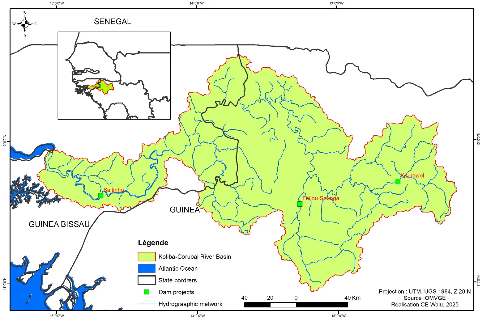
The Koliba/Corubal river basin lies between 11° N and 12°30′ N and between 12° W and 14°30′ W. It is shared between Guinea (84.5% of the area) and Guinea-Bissau (15.5%), covering 20,876.4 km2 at the Tché-Tché gauging station (Figure 1). The river originates in the western part of the Fouta Djallon highlands (Middle Guinea, Labé region). It forms from the confluence of two headwater streams: the Tomine (rising near Sangale) and the Kombia (rising near Madina Wora). These two tributaries meet near Gaoual to form the Koliba. After flowing westward for more than 200 km, the river briefly delineates the border between Guinea and Guinea-Bissau before entering the latter, where it is renamed the Corubal. It subsequently joins the Kayanga/Geba River near Xime in a flat, marshy zone where tidal influences extend far inland, creating the Geba estuary [2,12]. Despite its relatively small catchment, this river constitutes Guinea-Bissau’s primary source of freshwater. For clarity, the dense hydrographic network has been simplified in Figure 1.
Vegetation within the basin includes dense forests, degraded montane forests, dry forests frequently affected by bushfires, wooded savannas, cultivated areas, and fallow lands [2,13]. The climate is tropical, characterized by a single rainy season lasting five months in the north and six months in the south, followed by a dry season (April to November), although minor rainfall (a few millimeters) may still occur during the dry period. Precipitation decreases from south to north in response to the West African monsoon. Average monthly maximum temperatures range from 26.0 °C to 33.4 °C in Labé and from 31.1 °C to 40.2 °C in Koundara (observed in August and April, respectively). Mean minimum temperatures vary between 10.2 °C and 18.3 °C in Labé and between 15.0 °C and 24.2 °C in Koundara from December to May.
2.1. Data Requirements
Operating the GR4J model over a catchment requires several input variables: the basin area (km2), daily precipitation (P), and daily potential evapotranspiration (E). These variables are required to estimate runoff at the basin outlet, which is the primary model output.
Daily maximum (Tmax) and minimum (Tmin) temperatures, together with precipitation data for the period 1981–1993, were extracted from CHIRPS (precipitation) and ERA5 (temperature) datasets. To compute the spatial average of rainfall over the Koliba-Corubal basin at the Tché-Tché station, the Thiessen polygon method was applied—a standard technique for merging data from multiple rain gauges.
Potential evapotranspiration (PET) was estimated using the Oudin method, which builds upon the Jensen-Haise and McGuinness formulations. This approach accounts for mean daily temperature, solar radiation, latitude, and day length, thereby providing a robust PET estimate over the modeling period.
2.2. Presentation of the GR4J Model
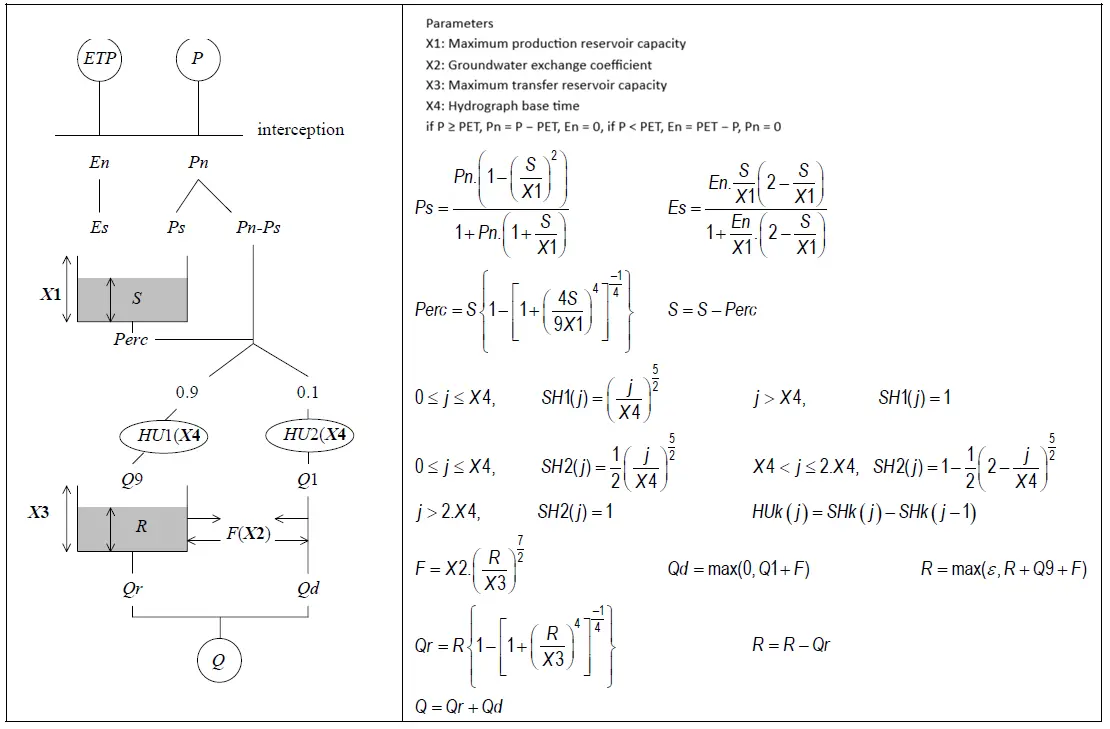
The GR4J model discretizes a catchment into sub-basins (Figure 2). For each sub-basin, net precipitation (Pn) or net evaporation (En) is determined by comparing precipitation (P) and potential evapotranspiration (E). When P exceeds E, net precipitation equals P − E and net evaporation is zero; conversely, when P is less than E, net evaporation equals E − P and net precipitation is zero. The model then routes water through two reservoirs (a production store and a routing store) to simulate streamflow at the outlet (Figure 2 retained as original).
2.3. Evaluation of Model Performance
Model accuracy improves when simulated discharges (Qc) closely match observed values (Qo). Comparing these two time series serves to evaluate model validity [14]. As noted by Hamby [15], such comparisons aid both model development and validation while minimizing uncertainties. Agreement between modelled hydrographs and field-measured data further confirms reliability.
2.3.1. The Nash Q Index
To assess the agreement between observed and simulated flows, we used the Nash-Sutcliffe efficiency (NSE), defined as [16,17]:
|
```latexNash\,(Q) = 1 - \dfrac{\sum_{i=1}^{n} \left(Q_{sim} - Q_{obs}\right)^2}{\sum_{i=1}^{n} \left(Q_{obs} - \bar{Q}_{obs}\right)^2}``` |
(1) |
where: Qsim is the simulated flow rate; Qobs is the observed flow rate; n is the number of time steps; and $$\bar{Q}_{obs}$$ is the average of the observed flow rates in the series.
The Nash–Sutcliffe efficiency ranges from 0 to 1, where 1 signifies perfect agreement between observed and simulated flows. A negative value indicates that the mean of observations provides a better prediction than the model [16]. This metric quantifies model accuracy based on residuals.
2.3.2. The Square Root of the Nash Index
This is the square root of the flows. This criterion is more sensitive to average flows. Its equation is 2 [16,17]:
|
```latexNash\,\left(\sqrt{Q}\right) = 1 - \dfrac{\sum_{i=1}^{n}\sqrt{\left(Q_{sim} - Q_{obs}\right)^2}}{\sum_{i=1}^{n}\sqrt{\left(Q_{obs} - \bar{Q}_{obs}\right)^2}}``` |
(2) |
2.3.3. The Natural Logarithm of the Nash Index
|
```latexNash\,\left(ln Q\right) = 1 - \dfrac{\sum_{i=1}^{n}\left(\ln Q_{obs} - ln Q_{sim}\right)^2}{\sum_{i=1}^{n}\left(\ln Q_{obs} - ln \bar{Q}_{obs}\right)^2}``` |
(3) |
The combined use of the Nash, R2, NSE, and PBIAS criteria allows the performance of the model to be evaluated. According to the Nash criterion, if Nash > 0.9, the model is excellent; between 0.80 and 0.90, it is very satisfactory; between 0.60 and 0.80, it is satisfactory; and if Nash < 0.60, it is poor. Reeda et al. [18] consider performance to be “satisfactory” if R2 > 0.60, NSE > 0.50 and PBIAS ≤ ±0.15, particularly for river or watershed-scale models.
2.3.4. Assessment of Uncertainties Associated with Simulated Flow Values
Hydrological model outputs inevitably carry uncertainty, a fact that must be clearly communicated. While conventional metrics, such as the Nash-Sutcliffe efficiency, measure absolute differences between observed and simulated flows, this approach treats all deviations equally. However, an error tolerable during floods may be unacceptable during low-flow periods. Accordingly, a ratio-based indicator (observed/simulated) offers a more diagnostically relevant alternative.
The model’s effectiveness is assessed by comparing simulated and observed flows using the Nash-Sutcliffe efficiency. A value close to 1 indicates good agreement, while a criterion below 60% indicates poor agreement. As the Nash-Sutcliffe efficiency is dimensionless, it allows models from different basins to be compared, regardless of their flow amplitudes. The performance of the model is first evaluated during calibration (1988–1993) and then validated for the period 1982–1987 in order to test its robustness under various conditions.
2.4. Model Calibration/Validation Method
Assessing the reliability of a hydrological model such as GR4J typically involves comparing simulated discharges against observed streamflow records. The most widely adopted metric for this purpose is the Nash-Sutcliffe efficiency (NSE), a dimensionless statistical indicator that measures how well simulated and observed flow curves agree. Because it has no units, the NSE enables direct performance comparisons across catchments with contrasting hydrological regimes—for instance, between a flashy, highly variable river and a stable, baseflow-dominated system.
A Nash value approaching 1 (100%) indicates an excellent match between simulations and observations, indicating that the model accurately reproduces the basin’s hydrological behavior. Conversely, an NSE below 0.6 (60%) suggests a poor fit, which may stem from incorrect parameter estimates, biases in input data (e.g., precipitation or evapotranspiration), or key hydrological processes not represented by the model structure.
In the present study, model evaluation follows a three-step procedure. First, a warm-up period of 365 days (the year 1981) initializes the model’s storage reservoirs. Second, calibration is performed over the 1988–1993 period, during which model parameters are adjusted to best replicate observed flows. Third, validation is carried out over an independent period (1982–1987). This final step is critical because it tests the model’s ability to predict flows under climatic and hydrological conditions that differ from those encountered during calibration. A model that performs well on both periods is considered robust.
By combining calibration and validation assessments through the Nash criterion, researchers obtain a powerful diagnostic tool. This approach ensures the model can be used confidently for future simulations or operational forecasting, provided the underlying assumptions remain valid.
2.5. Data and Methods Used for Future Hydrological Trends
Once the GR4J model was successfully calibrated and validated, we assessed the influence of projected changes in precipitation and temperature on future water availability. Bias-corrected outputs from CMIP6 models were used as input to GR4J. Correction was performed using the modified quantile mapping method: for temperature, the difference (additive) method; for precipitation, the multiplicative (delta) method. After bias correction, the multi-model ensemble mean showed a correlation coefficient >0.95 for temperature and >0.60 for precipitation relative to observed data in the basin. Using the ensemble mean helped to reduce inter-model divergence.
Although the bias-corrected multi-model ensemble achieved a monthly precipitation correlation of 0.60, this value is consistent with previous hydrological impact studies conducted in West Africa, which reported correlations between 0.55 and 0.65 [19]. This level of correlation may therefore be acceptable for runoff simulation and consideration.
To ensure reliable projections, simulated CMIP6 results were compared with historical observations in the Koliba-Corubal basin. Four GCMs that accurately reproduce past precipitation according to Saley & Salack [19] and Zarrin & Dadashi-Roudbari [20] were selected: GFDL-ESM4, MPI-ESM1-2-HR, UKESM1-0-LL, and IPSL-CM6A-LR (Table 1). Daily maximum/minimum temperatures and monthly accumulated precipitation were downloaded in CSV format.
Table 1. Some characteristics of the four climate models selected.
|
GCM Name |
Institute/Country |
Variant ID |
Horizontal Resolution |
Country |
|---|---|---|---|---|
|
IPSL-CM4A-MR |
Pierre Simon Laplace Institute |
r1i1p1f1 |
2.50° × 1.26° |
France |
|
MPI-ESM1-2-HR |
Max Planck Institute for Meteorology |
r1i1p1f1 |
0.94° × 0.94° |
Germany |
|
GFDL-ESM4 |
Geophysical Fluid Dynamics Laboratory |
r1i1p1f1 |
1.25° × 1.00° |
USA |
|
UKESM1-0-LL f2 |
National Institute of Meteorological Sciences/Korea Meteorological Administration |
r1i1p1f1 |
1.875° × 1.25° |
New Zealand |
We assumed that the precipitation-runoff relationship derived from historical data would remain stationary (no major land-use changes). GR4J was then used to generate daily flow series for the past (historical) and future (2015–2100), divided into three 30-year periods: near future (2021–2050), mid-century (2051–2080), and far future (2071–2100). Trend analysis was performed using Mann-Kendall and Pettitt tests. Relative seasonal (or interannual) change rates were calculated as the difference between each future period and the historical baseline (1985–2014).
3. Results
3.1. Variability of Observed and Simulated Flows During Wet and Dry Sub-Periods in Calibration and Validation with the GR4J Model Using Different Nash Criteria
The evaluation of the GR4J model’s performance was carried out by comparing observed and simulated daily discharges at the Tché-Tché station over two distinct periods: calibration (1988–1993) and validation (1982–1987). Figure 3 and Figure 4 illustrate the temporal evolution of precipitation inputs and the corresponding hydrographs. The analysis of rainfall patterns (Figure 3) reveals interannual and seasonal fluctuations that strongly influence runoff generation. Understanding the distribution and intensity of precipitation is essential for correctly interpreting the model’s ability to replicate the basin’s hydrological response.
Figure 4 presents a side-by-side comparison of measured versus modelled flows. Visual inspection shows that the GR4J model captures the overall shape of the hydrograph, though some peak events are underestimated, particularly during high-rainfall years. This visual assessment helps identify systematic biases in the simulated outputs.
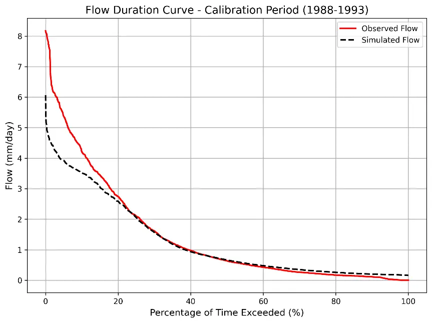
Figure 5 displays the flow duration curves (FDC) for both calibration and validation periods. The FDC for the calibration phase shows a closer match between observed and simulated flows than the validation phase, indicating that the parameter set optimized during calibration performs reasonably well, but with a slight loss of accuracy when applied to an independent period.
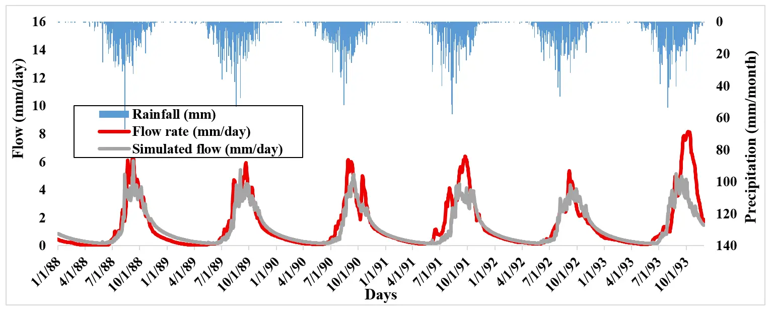
Figure 3. Daily hydrograph of observed and simulated flows for the calibration period (1988–1993) at the Tche Tche gauging station.
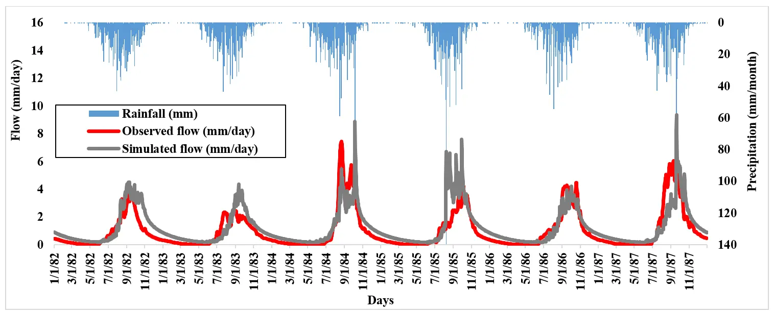
Figure 4. Daily hydrograph of observed and simulated flows for the validation period (1982–1987) at the Tche Tche gauging station.
 |
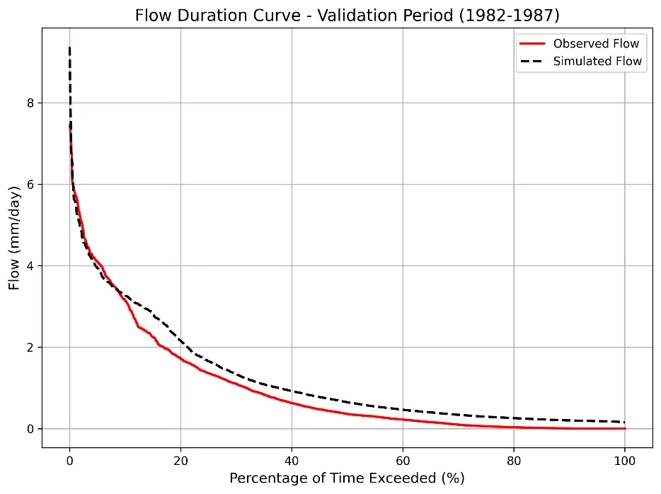 |
Figure 5. Flow duration curves comparing observed and simulated flows during the calibration (1988–1993) and validation (1982–1987) periods at the Tche Tche gauging station.
Figure 6 presents scatter plots of observed versus simulated flows, along with the corresponding correlation coefficients and performance metrics summarized in Table 2. During calibration, the correlation coefficient (R) reached 0.779, while the mean Nash-Sutcliffe efficiency (NSE) was 70.0%. For the validation period, R dropped to 0.667 and the mean NSE to 65.3%. These values indicate that the model performs satisfactorily in both phases, albeit with better performance during calibration.
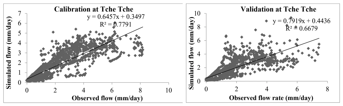
Figure 6. Scatter plots of observed flow versus simulated flow for the calibration period (1988–1993) and validation period (1982–1987) at the Tche Tche gauging station.
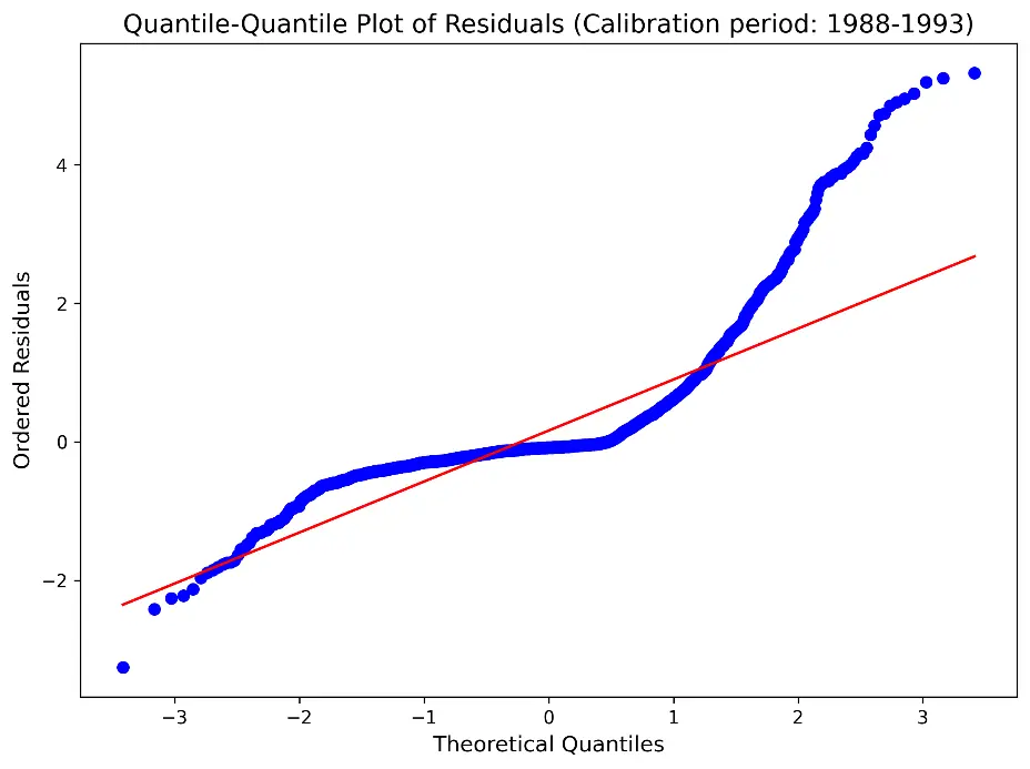
A quantile-quantile (QQ) plot (Figure 7) was used to compare the two probability distributions of observed and simulated flows. The deviation of points from the 1:1 reference line indicates a systematic bias in the sample.
 |
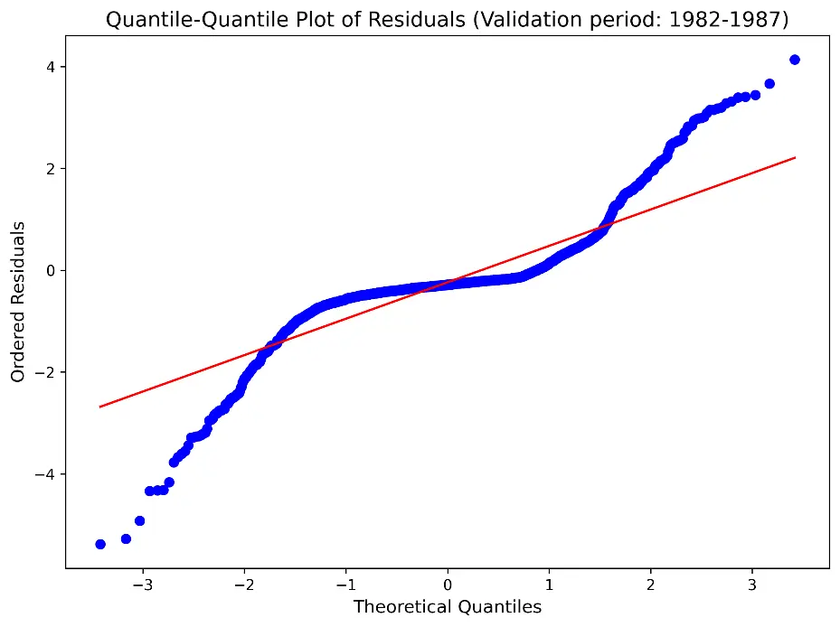 |
Figure 7. Quantile-quantile plot of observed flow residuals versus simulated flow for the calibration (1988–1993) and validation (1982–1987) periods at the Tche Tche gauging station.
Table 2 summarizes the performance metrics of the GR4J model during calibration (1988–1993) and validation (1982–1987) at the Tché-Tché station. Three variants of the Nash-Sutcliffe criterion were considered: Nash (Q), Nash ($$\sqrt{\mathrm{Q}}$$), and Nash (ln Q).
Table 2. Model performance criteria during the calibration period (1988–1993) and validation period (1982–1987) at the Tche Tche gauging station.
|
Calibration Period (1988–1993) |
Efficiency Criteria |
|---|---|
|
Nash (Q) |
0.70 |
|
Nash ($$\sqrt{\mathrm{Q}}$$) |
0.77 |
|
Nash (ln Q) |
0.63 |
|
Balance |
1.03 |
|
Validation Period (1982–1987) |
Efficiency Criteria |
|
Nash (Q) |
0.69 |
|
Nash ($$\sqrt{\mathrm{Q}}$$) |
0.73 |
|
Nash (ln Q) |
0.54 |
|
Balance |
1.18 |
During calibration, the values obtained for Nash (Q), Nash ($$\sqrt{\mathrm{Q}}$$), and Nash (ln Q) were 0.70, 0.77, and 0.63, respectively. For the validation period, the corresponding values were 0.69, 0.73, and 0.54. These scores reflect a reasonably satisfactory agreement between observed and modelled discharges across both time windows.
The Nash (Q) and Nash ($$\sqrt{\mathrm{Q}}$$) criteria yielded results close to acceptable thresholds, confirming the model’s ability to represent both high-flow and low-flow conditions effectively. Notably, the Nash (ln Q) criterion—which is particularly sensitive to low-flow dynamics—showed values of 0.63 during calibration and 0.54 during validation, indicating adequate performance during dry periods.
The Nash ($$\sqrt{\mathrm{Q}}$$) criterion, which provides a balanced evaluation between average flows and flood peaks, demonstrated robust results (0.77 for calibration, 0.73 for validation). This confirms the model’s strong capability to simulate hydrological behavior under both normal and extreme regimes. Overall, the performance criteria obtained for both periods validate the model’s acceptable skill and confirm a good correspondence between observed and simulated flow series.
The uncertainty assessment, based on the ratio, gave values of 1.03 during calibration (1988–1993) and 1.18 during validation (1982–1987). Both indicate that the GR4J model slightly underestimates observed flows at the Tché-Tché station. Correlation and efficiency coefficients remained comparable across the two periods.
Model performance varied depending on the objective function applied. The Nash function applied to the logarithm of flows, NSE (ln Q), produced the largest volume bias in both phases. Conversely, the standard Nash function based on discharge (NSE on Q) yielded the most accurate estimates of daily flows, peak timing, and volumetric ratios. This finding aligns with earlier calibration studies of African catchments, in which NSE (Q) consistently outperformed other formulations.
Despite a general tendency toward underestimation, the model delivered better absolute results during validation than during calibration when NSE (Q) was used. However, certain high-flow events were not well reproduced, notably in 1993 (calibration) and 1985 (validation), as shown in Table 3 and Figure 4.
Table 3. Average flows observed and simulated (mm) by the GR4J model during the calibration (1982–1987) and validation (1988–1993) periods at the Tche Tche gauging station.
|
Period |
Calibration (1988–1993) |
Validation (1982–1987) |
||||
|---|---|---|---|---|---|---|
|
Observed Flow |
Simulated Flow |
Difference |
Observed Flow |
Simulated Flow Rate |
Difference |
|
|
Average flow rate |
1.45 |
1.28 |
0.16 |
0.99 |
1.22 |
−0.24 |
The observed volume discrepancies largely reflect differences in hydrological conditions between the two periods. The mean observed annual flow was 1.45 mm during calibration, but fell to 0.99 mm during validation. The simulated averages were 1.28 mm (calibration) and 1.22 mm (validation), corresponding to a deviation of −0.16 mm and +0.24 mm, respectively. Thus, the model underestimated during the wetter calibration period and overestimated during the drier validation period, highlighting its sensitivity to interannual climate variability.
Table 4 shows that the correlation between observed and simulated flows reaches 0.779 during calibration and 0.667 during validation, indicating satisfactory model performance in both periods despite a slight decline in the independent phase. Mean model efficiencies are 70.0% (calibration) and 65.3% (validation), confirming that the GR4J model reliably reproduces daily discharge dynamics. Bias analysis reveals small but discernible deviations: an underestimation of 0.16 mm during calibration, and an overestimation of −0.24 mm during validation. These opposing biases suggest that the model responds to differences in climatic forcing between the two periods, particularly higher rainfall amounts recorded during validation. Overall, the GR4J model demonstrates acceptable robustness for simulating flows in the Koliba-Corubal basin. However, the systematic shift in bias from negative to positive indicates that some parameters could be refined to improve transferability under varying moisture conditions. Future calibration strategies might benefit from multi-objective approaches that explicitly balance performance across wet and dry sub-periods.
Table 4. Correlation between observed and simulated flows, average performance, and calibration and validation uncertainties during the calibration period (1982–1987) and validation period (1988–1993) at the Tche Tche gauging station.
|
Parameters |
Calibration |
Validation |
|---|---|---|
|
Correlation coefficient |
0.779 |
0.667 |
|
Average performance (%) |
70.0 |
65.3 |
|
Average deviation in mm |
0.16 |
−0.24 |
3.2. Future Hydrological Trends in the Koliba-Corubal Basin
3.2.1. Annual-Scale Evolution
To project climate change impacts and hydrological response in the Koliba-Corubal basin, CMIP6 scenarios (SSP126, SSP370, SSP585) were coupled with the GR4J model. Mann-Kendall and Pettitt tests were applied to future flow series (2021–2100) to detect trends and potential breakpoints. Results are summarized in Table 5 and Figure 8.
Table 5. Mann Kendall, and Pettitt test values for average annual water flow over the future period (2021–2100) in the Koliba Corubal basin at a risk of error of 0.05.
|
Mann Kendall Test |
Pettitt Test |
||||||
|---|---|---|---|---|---|---|---|
|
Flows |
Kendall’s Tau |
p-Value |
Sen Slope |
Year of Rupture |
Average Before Break |
Average After Break |
Percentage Change |
|
SSP 126 |
0.17 |
0.0238 |
0.00 |
2085 |
1.3 |
1.6 |
21.4 |
|
SSP 370 |
−0.68 |
0.0000 |
−0.01 |
2057 |
1.2 |
0.7 |
−42.1 |
|
SSP 585 |
−0.59 |
0.0000 |
−0.01 |
2057 |
1.2 |
0.7 |
−42.4 |
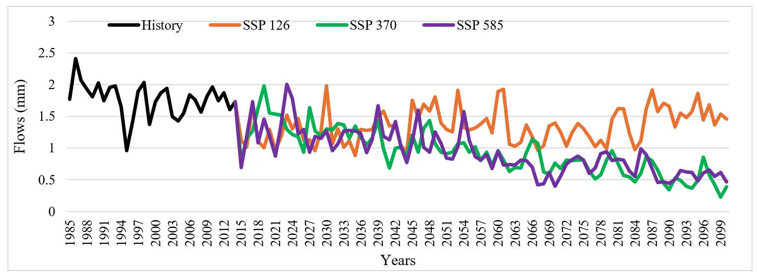
Figure 8. Evolution of annual flows over the historical period and the future period according to scenarios in the Koliba Corubal basin.
The Mann-Kendall test reveals that the flow trends for the three scenarios are contrasting. Under the SSP 126 scenario, there is a slight increase of 0.17 (positive Kendall’s Tau), indicating an upward trend in flows, with a significant p-value of 0.0238. In contrast, under the SSP 370 and SSP 585 scenarios, the negative Kendall’s Tau values (−0.68 and −0.59, respectively) indicate downward trends, with very low p-values (0.00), confirming a significant trend of decreasing flows in the future.
The Pettitt test confirms these results, indicating a break in 2085 for SSP 126, where the average flow rate increases from 1.3 to 1.6, a variation of 21.4%. However, under SSP 370 and SSP 585, the break occurs earlier (in 2057), and the averages before and after the break decrease, with a drastic drop of 42.1% under SSP 370 and 42.4% under SSP 585.
Overall, the tests indicate a persistent downward trend in basin flows, particularly under SSP 370 and SSP 585. This confirms the vulnerability of water resources to climate change, with the most pessimistic scenarios predicting a collapse in flows by 2100.
Figure 8 presents flow forecasts for the Koliba-Corubal basin over different future periods (near, medium, and distant) based on the three climate scenarios SSP 126, SSP 370, and SSP 585, compared to the reference period 1985–2014.
Over the period 2021–2050, flow under the SSP 126 scenario decreases slightly by −25.16%, while under SSP 370 and SSP 585, the reductions are −32.2% and −31.3%, respectively (Table 6). Compared to the SSP 126 scenario, SSP 370 shows a more pronounced decline, suggesting that high greenhouse gas emissions (SSP 370) would lead to a greater reduction in water resources. For the period 2051–2080, the trend continues with an even greater reduction in the SSP 370 and SSP 585 scenarios. The decreases are −53.2% and −55.2%, respectively, while SSP 126 shows a moderate reduction of −26.8%. Finally, for the period 2071–2100, the SSP 585 scenario reveals an even more pronounced decrease in flows, with a drop of −65.6%, while SSP 126 remains relatively more stable with a reduction of −20%.
Thus, the SSP 370 and SSP 585 scenarios predict a significant reduction in flows in the future, which could seriously affect water resources in the Koliba-Corubal basin.
Table 6. Future changes in flow rates (in %) on an annual basis over the three future periods according to the SSP126, SSP370 and SSP585 scenarios in the Koliba Corubal basin.
|
Flow |
1985–2014 |
2021–2050 |
Variation in % |
2051–2080 |
Variation in % |
2071–2100 |
Variation in % |
2021–2100 |
Variation in % |
|---|---|---|---|---|---|---|---|---|---|
|
SSP 126 |
1.8 |
1.3 |
−25.16 |
1.3 |
−26.8 |
1.4 |
−20.0 |
1.4 |
−22.98 |
|
SSP 370 |
1.8 |
1.2 |
−32.2 |
0.83 |
−53.2 |
0.61 |
−65.6 |
0.89 |
−49.4 |
|
SSP 585 |
1.8 |
1.2 |
−31.3 |
0.8 |
−55.2 |
0.7 |
−61.7 |
0.91 |
−48.5 |
According to the model outputs, the Koliba-Corubal basin’s flow regime could undergo substantial changes over the next several decades (Figure 9), with lower runoff volumes becoming more likely under selected climate pathways. Additionally, the basin’s hydrological feedback, as simulated by the GR4J model, shows that ongoing warming will amplify evapotranspiration rates, particularly by the end of the century, while precipitation simultaneously decreases.
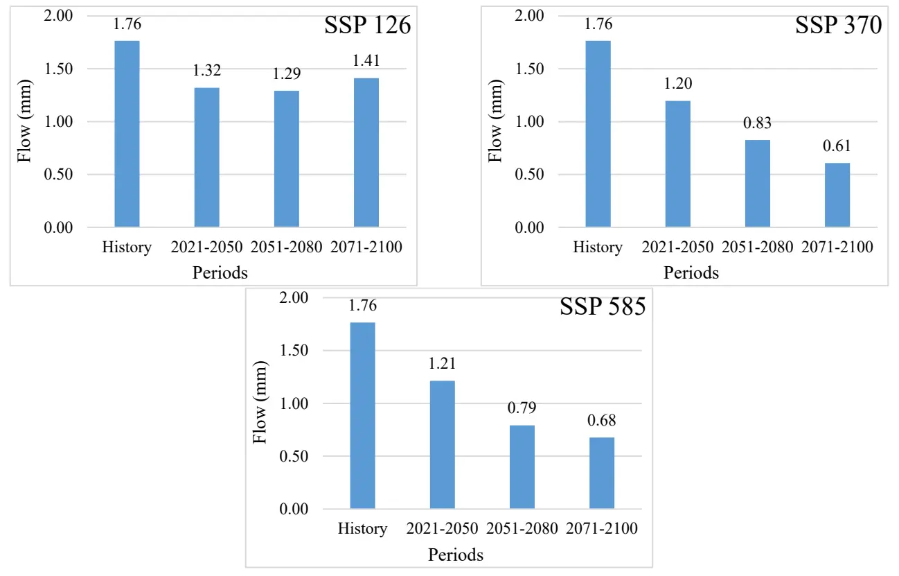
Figure 9. Comparison between the observed historical average flow and the simulated flow in climate change scenarios in the Koliba Corubal basin.
Projected hydrological trajectories for the Koliba-Corubal basin point toward altered flow regimes in the decades ahead. Under several emission pathways, simulations consistently indicate a transition to reduced discharge levels. The application of conceptual runoff models reveals an intensification of evaporative losses as temperatures rise, particularly pronounced during the late 21st century. This enhanced atmospheric water demand occurs concurrently with declining rainfall amounts. The combined effect of these two drivers—lower precipitation input and higher evapotranspiration rates—reinforces the likelihood of diminished water availability. Such feedback mechanisms within the basin’s hydrological system suggest that drier conditions will become more frequent and severe, especially under high-emission scenarios. These findings underscore the need to anticipate shifts in seasonal flow distribution and to prepare for prolonged low-flow periods that may challenge water supply reliability for human and agricultural use.
3.2.2. Monthly Trends
Table 7 and Figure 10 show the simulated average monthly flows in the Koliba-Corubal basin using climate model projections applied to the GR4J hydrological model, comparing the reference periods (1985–2014) and future projections (2021–2100) under three emission scenarios: SSP 126, SSP 370, and SSP 585.
Table 7. Simulated flow values on a monthly basis for the reference period (1985–2014) and the future period (2021–2100) in the Koliba Corubal basin (mm).
|
Parameters |
J |
F |
M |
A |
M |
J |
J |
A |
S |
N |
N |
D |
|---|---|---|---|---|---|---|---|---|---|---|---|---|
|
History |
0.9 |
0.7 |
0.5 |
0.4 |
0.3 |
0.6 |
1.5 |
3.7 |
5.3 |
3.9 |
2.1 |
1.3 |
|
SSP 126 |
0.7 |
0.5 |
0.4 |
0.3 |
0.2 |
0.3 |
0.7 |
2.5 |
4.5 |
3.3 |
1.8 |
1.1 |
|
SSP 370 |
0.6 |
0.4 |
0.3 |
0.2 |
0.2 |
0.2 |
0.4 |
1.2 |
2.9 |
2.3 |
1.3 |
0.8 |
|
SSP 585 |
0.6 |
0.4 |
0.3 |
0.2 |
0.2 |
0.2 |
0.4 |
1.2 |
2.8 |
2.5 |
1.3 |
0.8 |
Comparing historical flows with future scenarios, we observe a decrease in flows in most months, particularly under the SSP 370 and SSP 585 scenarios. In January, February, and March, flows under future scenarios are lower than in the historical period, with a more marked reduction in the SSP 370 and SSP 585 scenarios. For example, the January flow rate drops from 0.9 mm in the historical period to 0.6 mm under the SSP 370 and SSP 585 scenarios. This trend continues until June, when flow rates remain relatively low in all three future scenarios, with a notable decrease in July and August.
Monthly flows under the SSP 126 scenario show a slight reduction compared to historical values, but the decline is less pronounced. In contrast, the SSP 370 and SSP 585 scenarios predict more significant decreases in flows, with particularly low values in April, May, and June, when flows drop to 0.2 mm in the SSP 370 and SSP 585 scenarios.
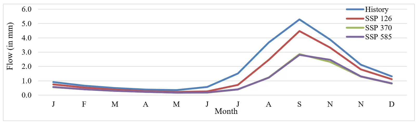
Figure 10. Change in simulated average monthly flows over the reference period (1985–2014) and the future period (2021–2100) in the Koliba Corubal basin.
For the Koliba-Corubal basin, the SSP3-7.0 and SSP5-8.5 scenarios both indicate sharply lower monthly discharges, especially during the dry season, posing serious challenges for regional water management.
Figure 11 shows the evolution of average monthly flows in the Koliba-Corubal basin under climate scenarios SSP 126, SSP 370, and SSP 585 for the three future horizons. Analysis of flows over the three future periods in the Koliba-Corubal basin under the SSP1-26, SSP3-70, and SSP5-85 scenarios reveals significant variations compared to the reference period. In the SSP 126 scenario, average monthly flows decrease gradually over time, particularly between 2021 and 2080. For example, flows from January 2021 to 2050 start at 0.734 mm and gradually decline under all three scenarios. In 2051–2080, this trend intensifies with average flows of 0.7271 mm for SSP 126, compared to 0.5202 mm for SSP 370 and 0.5133 mm for SSP 585.
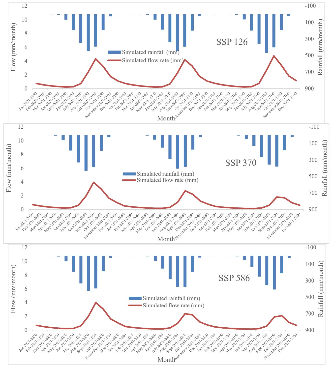
Figure 11. Variation in future flow simulated by the GR4J model for the period 2021–2100 in the Koliba Corubal basin, according to climate change scenarios for the future period.
Under the SSP 370 scenario, the decrease is less pronounced compared to SSP5-85. This indicates that future temperature and humidity will have significant impacts, particularly in reducing flows over the entire period. In contrast, the SSP 585 scenario predicts a greater decline, indicating more dramatic effects of climate change, with lower figures than those of the other scenarios. In 2071–2100, for example, monthly flows under SSP 585 fall to even lower levels, reaching values such as 1.9006 mm in September 2071–2100. This general trend of decreasing flows illustrates the increased vulnerability of the Koliba-Corubal basin to future climate change.
3.3. Summary Statistics, Autocorrelation, and Cross-Correlation for All Scenarios
To characterize the input and output data used in the GR4J model, we computed a set of descriptive statistics for all time series. Table 8 summarizes the main properties of historical precipitation and simulated discharge (1985–2014) as well as future projections (2015–2100) under SSP126, SSP370, and SSP585.
Table 8. Complete summary statistics for all hydroclimatic time series (historical and future scenarios).
|
Series |
Period |
Length (Years) |
% Zero |
% Missing |
Mean |
Variance |
Std Dev |
Skewness |
Kurtosis |
Auto_Corr(1) |
Auto_Corr(2) |
Cross_Corr(P,Q) |
|---|---|---|---|---|---|---|---|---|---|---|---|---|
|
Precipitation (historical) |
1985–2014 |
30 |
0% |
0% |
1668.5 |
14.789 |
121.6 |
−0.21 |
2.45 |
0.31 |
0.12 |
– |
|
Simulated discharge (historical) |
1985–2014 |
30 |
0% |
0% |
1.76 |
0.108 |
0.328 |
−0.25 |
2.78 |
0.45 |
0.22 |
0.78 |
|
Precipitation SSP126 |
2015–2100 |
86 |
0% |
0% |
1712.4 |
22.156 |
148.8 |
0.15 |
2.61 |
0.28 |
0.10 |
– |
|
Discharge SSP126 |
2015–2100 |
86 |
0% |
0% |
1.32 |
0.092 |
0.303 |
0.08 |
2.65 |
0.48 |
0.21 |
0.74 |
|
Precipitation SSP370 |
2015–2100 |
86 |
0% |
0% |
1568.9 |
19.834 |
140.9 |
0.22 |
2.54 |
0.26 |
0.09 |
– |
|
Discharge SSP370 |
2015–2100 |
86 |
0% |
0% |
0.83 |
0.088 |
0.297 |
0.42 |
2.89 |
0.52 |
0.24 |
0.69 |
|
Precipitation SSP585 |
2015–2100 |
86 |
0% |
0% |
1549.4 |
21,203 |
145.6 |
0.18 |
2.58 |
0.29 |
0.11 |
– |
|
Discharge SSP585 |
2015–2100 |
86 |
0% |
0% |
0.79 |
0.091 |
0.302 |
0.35 |
2.71 |
0.49 |
0.22 |
0.71 |
Mean: annual average (mm for precipitation, mm/year for discharge); Variance: measure of dispersion; Std Dev: standard deviation; Skewness: negative values indicate a left-tailed distribution (more high values), positive values indicate a right-tailed distribution (more low values); Kurtosis: value of 3 corresponds to a normal distribution; Auto_corr(1): autocorrelation at lag 1 (one year); Auto_corr(2): autocorrelation at lag 2 (two years); Cross_corr(P,Q): cross-correlation between precipitation and discharge at lag 0 (simultaneous relationship).
The statistical summary reveals distinct differences between historical and future hydrological regimes across the three SSP scenarios.
Historical period (1985–2014): Precipitation shows a near-normal distribution with slight negative skewness (−0.21) and kurtosis of 2.45, indicating a mild tail toward higher rainfall years. Simulated discharge exhibits a mean of 1.76 mm/year, negative skewness (−0.25), and moderate autocorrelation at lag-1 (0.45), suggesting some interannual persistence. The cross-correlation between precipitation and discharge reaches 0.78, confirming a strong linear rainfall-runoff relationship.
Future scenarios (2015–2100): Under SSP126, precipitation increases slightly (mean 1712.4 mm) while discharge declines to 1.32 mm/year. Skewness becomes slightly positive (0.08–0.15), indicating a shift toward more frequent low-flow years with occasional wet extremes. Autocorrelation at lag-1 rises to 0.48–0.52 under SSP370 and SSP585, implying greater hydrological persistence and longer dry spells. This is critical because the basin already experiences marked dry seasons.
Cross-correlations remain high (0.69–0.74), demonstrating that the GR4J model preserves a coherent precipitation-runoff relationship under climate change. However, the decline in mean discharge from 1.76 (historical) to 0.79–1.32 mm/year represents a 25–55% reduction, with the strongest drying under SSP585.
Kurtosis values remain near 3 across all series, suggesting that extreme events are not disproportionately more frequent than the mean. However, positive skewness in future discharge (up to 0.42 under SSP370) indicates an asymmetric distribution with a longer tail toward low flows.
In summary, the statistics confirm that the Koliba-Corubal basin is transitioning toward drier, more persistent low-flow conditions, particularly under high-emission scenarios, while maintaining strong coupling between rainfall and runoff.
4. Discussion of Results
Grasping how climate change affects water cycles is critical for managing water resources in sensitive zones like the Koliba-Corubal catchment. Using the GR4J model with historical weather data (1981–1993) and CMIP6 future projections (SSP1-2.6, SSP3-7.0, SSP5-8.5), this research simulates runoff responses. The results point to declining rainfall and sharply rising temperatures by 2100 [21,22], reinforcing the need for anticipatory water management strategies in this vulnerable region.
The results of the modeling show that the Koliba-Corubal basin will be affected by an increase in the number of dry years, with a reduction in water resources, particularly during dry periods, when the frequency and intensity of droughts are expected to increase. Climate models predict a decrease in rainfall, exacerbated by increased evapotranspiration caused by rising temperature [5,23,24,25]. This trend toward aridification is part of a broader context of climate change, where areas such as West Africa, and more particularly the Koliba-Corubal basin, are increasingly vulnerable to extreme weather events, particularly prolonged droughts [26,27].
Projections indicate that annual runoff in the basin will also be reduced, a trend confirmed by simulations carried out with the GR4J model, which used the same CMIP6 climate scenarios to assess future impacts on water resources. This reduction in runoff will directly affect water availability for agriculture and the drinking water supply [11]. In particular, reduced soil moisture and increased frequency of drought periods will put increased pressure on water resources, making their management even more complex in the future [10,28].
The results of this study, which combine climate scenarios and hydrological modelling data, are consistent with those of other research on West African watersheds. For example, studies conducted in the Gambia River basin have also shown a significant reduction in flows due to decreased rainfall and increased evapotranspiration [25,26]. Furthermore, changes in rainfall patterns in this region will have major consequences for water resource management, particularly during the dry season, when intensified droughts could affect agricultural production, fisheries, and local biodiversity [29,30].
Modelling using the GR4J model shows that the three scenarios studied (SSP 126, SSP 370, and SSP 585) indicate a gradual reduction in average monthly flows, with a more marked decline under the SSP 585 scenario, indicating particularly severe effects of climate change [28]. Although the GR4J model is relatively simple and useful for global simulations, it is clear that more detailed, distributed models better suited to the watershed scale would be needed to obtain more accurate projections and take into account local specificities [10].
Finally, although climate model projections based on future warming scenarios show converging results, these simulations also involve uncertainties, mainly due to the quality and resolution of the climate data used. Coarse-resolution climate models (~200 km) do not always capture the local characteristics of smaller watersheds, which limits the accuracy of projections, particularly for smaller geographical scales [31]. These uncertainties must be taken into account when interpreting the results, as they may influence adaptation and water resource management strategies for the coming years.
This study highlights the increased vulnerability of the Koliba-Corubal basin to the effects of climate change, particularly reduced rainfall and increased temperatures, which will exacerbate droughts and limit available water resources. These results underscore the need to strengthen adaptation strategies to ensure sustainable water management in this basin by integrating climate change impacts into water resource management policies [22,32].
However, it is worth noting that the assumption that rising temperature systematically leads to decreasing precipitation is not universally valid, as other processes, such as changes in specific humidity rather than relative humidity, play a critical role in precipitation and runoff generation; indeed, while relative humidity has remained relatively stable globally despite warming, specific humidity has increased [33], and therefore a comprehensive analysis of trends in temperature, precipitation, specific humidity, and relative humidity is recommended before drawing firm conclusions about future climatic conditions in the study area.
Although our analysis is based on 13 years of historical climate data (1981–1993), due to the absence of measured runoff for the other years (the series being incomplete), we recognize that longer observation series (generally >30 years) are usually necessary to adequately capture the long-term statistical characteristics of temperature, precipitation, and streamflow processes, particularly in the presence of long-term persistence (LTP) behavior—characterized by a Hurst exponent H > 0.8—which induces intrinsic uncertainty across multiple timescales and can lead to prolonged clustering of wet and dry years, as documented in hydrological time series [34,35,36] and as suggested by the variability observed in our data (Figure 6).
As illustrated in Figure 3 and Figure 4, the GR4J model captures the overall seasonal variability of streamflow in the Koliba-Corubal basin; however, consistent with the findings of Blöschl et al. [37] for European catchments and Lins & Slack [38] for USGS records, our results show that climate-driven hydrological variability can lead to both increases and decreases in flow regimes depending on the period considered, which underscores the importance of non-stationarity in water resource assessment, a principle strongly advocated within the IAHS community [39].
In light of recent literature highlighting the limitations of the classical Mann–Kendall and Sen slope methods, particularly their sensitivity to serial correlation and long-term persistence (Hurst phenomenon), we acknowledge that these approaches may overestimate trend significance, and we therefore plan to apply the Hamed [40] variance correction method in future work to account for scaling effects, as recommended by Serinaldi et al. [41].
Although the GR4J model achieved satisfactory Nash-Sutcliffe efficiencies for overall daily flows (calibration: 0.70; validation: 0.69), its performance in reproducing low-flow periods was notably weaker. The Nash(ln Q) value of 0.54 during validation falls below the commonly accepted threshold of 0.60, indicating that the model struggles to simulate very low discharges accurately. This limitation is particularly relevant because our main conclusions concern projected reductions in dry-season flows. Consequently, while the direction of change (declining flows) is consistent across all SSP scenarios, the absolute magnitude of dry-season flow reduction should be interpreted with caution. The poor low-flow performance likely stems from the GR4J model’s simplified representation of groundwater storage and baseflow recession, as well as potential precipitation biases in the CHIRPS dataset during extended dry periods. Future work should consider using a distributed model (e.g., SWAT or HBV) or applying a specific low-flow bias correction to improve confidence in dry-season projections.
5. Conclusions
This research assessed how climate change may affect hydrological conditions in the Koliba-Corubal catchment (Guinea-Guinea-Bissau) by applying the GR4J rainfall-runoff model together with CMIP6 projections under three emission pathways (SSP1-2.6, SSP3-7.0, SSP5-8.5). The simulations indicate growing susceptibility of the basin to climatic pressures, especially declining precipitation and increasing temperatures. By 2100, river discharges are projected to drop substantially—most notably during dry months—accompanied by more frequent drought events, thereby threatening both domestic and agricultural water supplies.
Higher temperatures combined with lower precipitation could increase regional aridity, thereby reducing runoff. surface water and soil moisture, although this is not always the case. These results directly compromise agricultural productivity and the availability of drinking water. Our findings are consistent with previous research conducted in West Africa, which also reports reductions in water resources induced by climate change.
Although the GR4J model offered a valuable basin-wide assessment, its conceptual simplicity imposes limitations. Finer-scale, distributed hydrological models would likely yield more precise, locally relevant projections.
In conclusion, this study underscores the urgent need to embed climate scenarios into water management frameworks and to implement adaptation measures that bolster community resilience to forthcoming hydrological stresses. Sustainable management of water resources is essential to safeguard food security and reliable freshwater supply—not only in the Koliba-Corubal basin but also across other vulnerable zones in West Africa.
Statement of the Use of Generative AI and AI-Assisted Technologies in the Writing Process
During the preparation of this manuscript, the author(s) used Deepseek for the translation into English and the formatting of the article to the standards of the journal. After using this tool/service, the author(s) reviewed and edited the content as necessary and take full responsibility for the content of the published article.
Acknowledgments
The authors acknowledge the providers of the CHIRPS precipitation data, ERA5 temperature data, and the CMIP6 climate model outputs.
Author Contributions
Conceptualization, C.E.W. and C.F.; Methodology, C.E.W. and C.F.; Software, C.E.W.; Validation, C.E.W. and C.F.; Formal Analysis, C.E.W.; Investigation, C.E.W.; Resources, C.E.W. and C.F.; Data Curation, C.E.W.; Writing—Original Draft Preparation, C.E.W.; Writing—Review & Editing, C.F.; Visualization, C.E.W.; Supervision, C.F.; Project Administration, C.F.; Funding Acquisition, none.
Ethics Statement
Not applicable for studies not involving humans or animals.
Informed Consent Statement
Not applicable.
Data Availability Statement
The climate data used in this study (CHIRPS, ERA5, CMIP6) are publicly available from their respective repositories. The modeled flow data can be obtained from the corresponding author upon reasonable request.
Funding
This research received no external funding.
Declaration of Competing Interest
The authors declare that they have no known competing financial interests or personal relationships that could have appeared to influence the work reported in this paper.
References
- Ndehedehe CE. The water resources of tropical West Africa: Problems, progress, and prospects. Acta Geophys. 2019, 67, 621–649. DOI:10.1007/s11600-019-00260-y [Google Scholar]
- Sambou S, Dacosta H, Diouf RN, Diouf I, Kane A. Hydropluviometric Variability in Non-Sahelian West Africa: Case of the Koliba/Corubal River Basin (Guinea and Guinea-Bissau). Proc. Int. Assoc. Hydrol. Sci. 2020, 383, 171–183. DOI:10.5194/piahs-383-171-2020 [Google Scholar]
- Dione PM, Faye C, Mohamed A, Alarifi SS, Mohammed MA. Assessment of the impact of climate change on current and future flows of the ungauged Aga-Foua-Djilas watershed: A comparative study of hydrological models CWatM under ISIMIP and HMF-WA. Appl. Water Sci. 2024, 14, 163. DOI:10.1007/s13201-024-02219-x [Google Scholar]
- Gbode IE, Diro GT, Intsiful JD, Dudhia J. Current conditions and projected changes in crop water demand, irrigation requirement, and water availability over West Africa. Atmosphere 2022, 13, 1155. DOI:10.3390/atmos13071155 [Google Scholar]
- Waha K, Krummenauer L, Adams S, Aich V, Baarsch F, Coumou D, et al. Climate Change Impacts in the Middle East and Northern Africa (MENA) Region, and Their Implications for Vulnerable Population Groups. Reg. Environ. Change 2017, 17, 1623–1638. DOI:10.1007/s10113-017-1144-2 [Google Scholar]
- Mouelhi S. Vers une chaîne cohérente de modèles pluie-débit conceptuels globaux aux pas de temps pluriannuel, annuel, mensuel et journalier. Ph.D. Thesis, ENGREF/CEMAGREF, Paris, France, 2003. Available online: https://pastel.hal.science/tel-00005696 (accessed on 12 February 2026).
- Mouelhi S, Michel C, Perrin C, Andreassian V. Linking Stream Flow to Rainfall at the Annual Time Step: The Manabe Bucket Model Revisited. J. Hydrol. 2006, 328, 283–296. DOI:10.1016/j.jhydrol.2005.12.022 [Google Scholar]
- Zarrin A, Dadashi-Roudbari A. Evaluation of reanalysis-based, satellite-based, and “bias-correction”-based datasets for capturing extreme precipitation in Iran. Meteorol. Atmos. Phys. 2022, 134, 67. DOI:10.1007/s00703-022-00903-8 [Google Scholar]
- Guo Q, He Z, Wang Z. Long-term projection of future climate change over the twenty-first century in the Sahara region in Africa under four Shared Socio-Economic Pathways scenarios. Environ. Sci. Pollut. Res. 2023, 30, 22319–22329. DOI:10.1007/s11356-022-23813-z [Google Scholar]
- Kay AL, Griffin A, Rudd AC, Chapman RM, Bell VA, Arnell NW. Climate Change Effects on Indicators of High and Low River Flow Across Great Britain. Adv. Water Resour. 2021, 151, 103909. DOI:10.1016/j.advwatres.2021.103909 [Google Scholar]
- Diop SB, Ekolu J, Tramblay Y, Dieppois B, Grimaldi S, Bodian A, et al. Climate change impacts on floods in West Africa: New insight from two large-scale hydrological models. Nat. Hazards Earth Syst. Sci. 2025, 25, 3161–3184. DOI:10.5194/nhess-25-3161-2025 [Google Scholar]
- SOFRECO. Study of the Master Plan for the Integrated Development and Management of the Kayanga/Gêba and Koliba-Corubal River Basins, Water Resources and Needs and Options for Hydraulic and Hydro-Agricultural Development; SOFRECO: Dakar, Senegal, 1993; Volume 3, Annex B. [Google Scholar]
- Lemenkova P. Mapping coastal regions of Guinea-Bissau for analysis of mangrove dynamics using remote sensing data. Transylv. Rev. Syst. Ecol. Res. 2024, 26, 17–30. DOI:10.2478/trser-2024-0008 [Google Scholar]
- Makhlouf Z, Michel C. A two-parameter monthly water balance model for French watersheds. J. Hydrol. 1994, 162, 299–318. DOI:10.1016/0022-1694(94)90233-X [Google Scholar]
- Hamby DA. A review of techniques parameters sensitivity analysis of environmental models. Environ. Monit. Assess. 1994, 32, 135–154. DOI:10.1007/BF00547132 [Google Scholar]
- Dechemi N, Benkaci T, Issolah A. Modélisation des débits mensuels par les modèles conceptuels et les systèmes neuro-flous. J. Water Sci. 2003, 16, 407–424. DOI:10.7202/705515ar [Google Scholar]
- Faye C, Sow AA. Analyse de la variabilité des ressources en eau dans le bassin de la Falémé par modélisation hydrologique. 2014. Available online: https://www.researchgate.net/publication/321490992_Analyse_de_la_variabilite_des_ressources_en_eau_dans_le_bassin_de_la_Faleme_par_modelisation_hydrologique#fullTextFileContent (accessed on 8 February 2026).
- Redda MA, Wolde BB, Mohamed BH. A comprehensive analysis of water budget components and water yield in the upper awash sub-basin, Central Ethiopia using the SWAT model. Glob. J. Earth Sci. Eng. 2025, 12, 30–56. DOI:10.15377/2409-5710.2025.12.3 [Google Scholar]
- Saley IA, Salack S. Present and future of heavy rain events in the Sahel and West Africa. Atmosphere 2023, 14, 965. DOI:10.3390/atmos14060965 [Google Scholar]
- Zarrin A, Dadashi-Roudbari A. Projected changes in temperature over Iran by 2040 based on CMIP6 multi-model ensemble. Phys. Geogr. Res. 2021, 53, 75–90. DOI:10.22059/JPHGR.2021.308361.1007551 [Google Scholar]
- Odunmorayo MT, Alani BO, Adefisan EA. Projected change in occurrence and severity of heatwaves over West Africa as simulated by CMIP6 models. J. Disaster Sci. Manag. 2025, 1, 16. DOI:10.1007/s44367-025-00017-z [Google Scholar]
- Dione PM, Faye C, Sadio CAAS. Hydrological Impacts of Climate Change (Rainfall and Temperature) and Characterisation of Future Drought in the Aga Foua Djilas Watershed. Indones. J. Soc. Environ. Issues (IJSEI) 2023, 4, 353–375. DOI:10.47540/ijsei.v4i3.1218 [Google Scholar]
- Driouech F, ElRhaz K, Moufouma-Okia W, Arjdal K, Balhane S. Assessing Future Changes of Climate Extreme Events in the CORDEX-MENA Region Using Regional Climate Model ALADIN-Climate. Earth Syst. Environ. 2020, 4, 477–492. DOI:10.1007/s41748-020-00169-3 [Google Scholar]
- Olusegun CF, Awe O, Ijila I, Ajanaku O, Ogunjo S. Evaluation of dry and wet spell events over West Africa using CORDEX-CORE regional climate models. Model. Earth Syst. Environ. 2022, 8, 4923–4937. DOI:10.1007/s40808-022-01423-5 [Google Scholar]
- Séne SMK, Faye C, Pande CB. Assessment of current and future trends in water resources in the Gambia River Basin in a context of climate change. Environ. Sci. Eur. 2024, 36, 32. DOI:10.1186/s12302-024-00848-2 [Google Scholar]
- Sadio CAAS, Faye C, Pande CB, Tolche AD, Ali MS, Cabral-Pinto MMS, et al. Hydrological Response of Tropical River Basins to Climate Change Using the GR2M Model: The Case of the Casamance and Kayanga-Géva River Basins. Environ. Sci. Eur. 2023, 35, 113. DOI:10.1186/s12302-023-00822-4 [Google Scholar]
- Sadio CAS. Hydrological Characterisation and Water Resource Management in a Context of Climate Variability and Change: The Case of the Casamance Watershed Upstream of Kolda and the Kayanga-Géva Watershed Upstream of Wassadou. Ph.D. Thesis, Assane Seck University of Ziguinchor, Ziguinchor, Senegal, 2024. [Google Scholar]
- Gierszewski PJ, Habel M, Szmańda J, Luc M. Evaluating Effects of Dam Operation on Flow Regimes and Riverbed Adaptation to Those Changes. Sci. Total Environ. 2020, 710, 136202. DOI:10.1016/j.scitotenv.2019.136202 [Google Scholar]
- Moriasi DN, Zeckoski RW, Arnold JG, Baffaut C, Malone RW, Daggupati P, et al. Hydrologic and Water Quality Models: Key Calibration and Validation Topics. Trans. ASABE 2015, 58, 1609–1618. DOI:10.13031/trans.58.11075 [Google Scholar]
- Ndione M, Faty A, Nguirane M, Fall AN. Caractérisation du régime hydrologique du fleuve Gambie et sa variabilité dans un contexte de changement climatique en Afrique de l’ouest. In Proceedings of the Conférence Internationale IS Rivers 2025, Lyon, France, 30 June–4 July 2025. Available online: https://hal.science/hal-05190102/ (accessed on 12 February 2026).
- Amiot L, Dubreuil V, Launay J, Bardon E, Massa F, Keromnes E. Territorial Climate Diagnosis Focusing on Water Resources: Methodological Guide. Ph.D. Dissertation, LETG, CRESEB, Brittany Region, Rennes, France, 2021. [Google Scholar]
- Dione PM, Faye C, Tolche AD. Projection of Future Temperature and Precipitation in the Aga-Foua-Djilas Basin in Senegal Using the CMIP6 Multi-Model Ensemble. J. Mater. Environ. Sci. 2025, 16, 256–281. Available online: https://www.jmaterenvironsci.com/Document/vol16/vol16_N2/JMES-2025-1602016-Dione.pdf (accessed on 11 February 2026).
- Koutsoyiannis D. Revisiting the global hydrological cycle: Is it intensifying? Hydrol. Earth Syst. Sci. 2020, 24, 3899–3932. DOI:10.5194/hess-24-3899-2020 [Google Scholar]
- Hurst HE. Long-term storage capacity of reservoirs. Trans. Am. Soc. Civ. Eng. 1951, 116, 770–799. DOI:10.1061/TACEAT.0006518 [Google Scholar]
- Beran J, Feng Y, Ghosh S, Kulik R. Long-Memory Processes: Probabilistic Properties and Statistical Methods; Springer: Berlin/Heidelberg, Germany, 2013. DOI:10.1007/978-3-642-35512-7 [Google Scholar]
- Pizarro A, Dimitriadis P, Iliopoulou T, Manfreda S, Koutsoyiannis D. Stochastic Analysis of the Marginal and Dependence Structure of Streamflows: From Fine-Scale Records to Multi-Centennial Paleoclimatic Reconstructions. Hydrology 2022, 9, 126. DOI:10.3390/hydrology9070126 [Google Scholar]
- Blöschl G, Hall J, Viglione A, Perdigão RAP, Parajka J, Merz B, et al. Changing climate both increases and decreases European river floods. Nature 2019, 573, 108–111. DOI:10.1038/s41586-019-1495-6 [Google Scholar]
- Lins HF, Slack JR. Seasonal and Regional Characteristics of U.S. Streamflow Trends in the United States from 1940 to 1999. Phys. Geogr. 2005, 26, 489–501. DOI:10.2747/0272-3646.26.6.489 [Google Scholar]
- Montanari A, Young G, Savenije HHG, Hughes D, Wagener T, Ren LL, et al. “Panta Rhei—Everything Flows”: Change in hydrology and society—The IAHS Scientific Decade 2013–2022. Hydrol. Sci. J. 2013, 58, 1256–1275. DOI:10.1080/02626667.2013.809088 [Google Scholar]
- Hamed KH. Trend detection in hydrologic data: The Mann–Kendall trend test under the scaling hypothesis. J. Hydrol. 2008, 349, 350–363. DOI:10.1016/j.jhydrol.2007.11.009 [Google Scholar]
- Serinaldi F, Chebana F, Kilsby CG. Dissecting innovative trend analysis. Stoch. Environ. Res. Risk Assess. 2020, 34, 733–754. DOI:10.1007/s00477-020-01797-x [Google Scholar]