Low-Carbon Economic Dispatch for Offshore Wind-Solar Grid-Connected Systems Considering Source-Load Uncertainty and Carbon Emission Flow

Low-Carbon Economic Dispatch for Offshore Wind-Solar Grid-Connected Systems Considering Source-Load Uncertainty and Carbon Emission Flow
Qiang Gao 1,2 Le Gu 1 Zemin Mao 3,* Qingao Chen 4 Shaobo Shi 1 Junjie Liu 1 Yuehui Ji 1
Received: 02 April 2026 Revised: 10 April 2026 Accepted: 28 April 2026 Published: 12 May 2026

© 2026 The authors. This is an open access article under the Creative Commons Attribution 4.0 International License (https://creativecommons.org/licenses/by/4.0/).
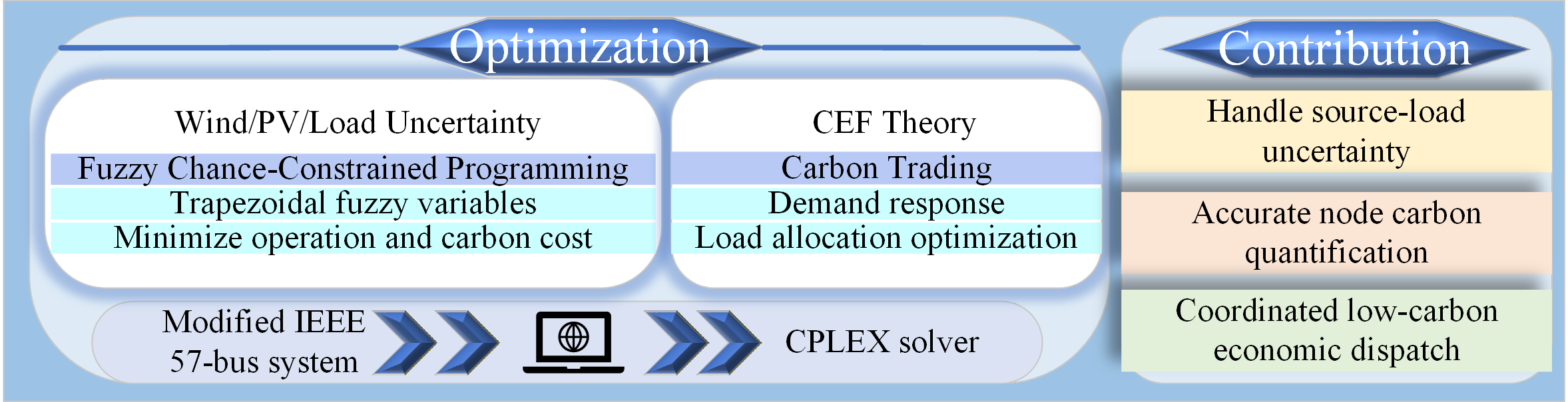
Graphical Abstract
1. Introduction
With abundant renewable energy resources such as wind and solar, offshore wind and offshore photovoltaic power serve as the core support for constructing modern marine energy systems [1]. These two sources complement each other in resource availability and output characteristics, effectively enhancing the reliability of power supply. Relying on vast marine space, they enable large-scale development without occupying terrestrial land resources, featuring high efficiency and environmental sustainability [2]. They can provide clean electricity for offshore platforms, islands, marine ranches, seawater desalination, deep-sea development, and other scenarios, thereby promoting fossil energy substitution and low-carbon transition [3]. Amid the continuous growth of global carbon emissions and intensifying climate warming, severe challenges have emerged for the sustainable development of human society [4]. To accelerate the process of carbon neutrality and achieve green transformation, the large-scale development and utilization of marine renewable energy, represented by offshore wind and offshore photovoltaic power, has become an inevitable strategic choice [5,6]. However, the inherent intermittency, volatility, and randomness of offshore wind and solar energy introduce considerable uncertainty into supply–demand distribution during large-scale grid integration, which seriously threatens the power balance, operational stability, and reserve allocation of marine power systems [7]. In particular, such uncertainty poses difficulties for accurate carbon emission quantification and for refined low-carbon regulation. Traditional dispatch methods usually rely on deterministic models or simple carbon accounting approaches, which cannot effectively capture the spatiotemporal carbon flow characteristics embedded in power flow, nor can they fully coordinate demand response to reduce carbon emissions from the load side. Moreover, the uncertainty of source–load variation is often handled separately from low-carbon dispatch, making it difficult to balance economy, low-carbon performance, and operational robustness simultaneously. To achieve green, secure, and economic operation of marine energy systems, research on low-carbon optimal dispatch has developed rapidly. Low-carbon dispatch requires comprehensive consideration of technical and economic factors from both the generation side [8] and the load side [9]. Therefore, in marine power systems with high renewable energy penetration, the coordinated optimization of economy, environmental protection, and operational safety has become one of the core issues that urgently need to be addressed [10,11].
1.1. Literature Review
The inherent volatility of offshore wind and marine solar photovoltaic resources, coupled with large deviations in marine load forecasting, represents critical factors that undermine the stable operation of marine power systems. Existing studies mainly tackle these uncertainty issues using three categories of methods: deterministic methods [12], stochastic programming [13], and fuzzy mathematics [14]. Deterministic methods dominated early research but neglected the dynamic nature of uncertainty. This tends to cause over-configuration of reserve capacity and cannot adapt to the intermittent fluctuations of offshore renewable energy output. Stochastic programming characterizes probability distributions (e.g., Weibull distribution [15]) of offshore wind, solar, and marine loads using historical data, and transforms uncertainty into probabilistic constraints embedded in dispatch models. However, stochastic programming relies heavily on the quality and quantity of historical data; insufficient data will significantly degrade the robustness of the model. Fuzzy mathematics describes uncertainty via fuzzy variables without predefining probability distributions, making it a research hotspot for handling uncertainty in recent years [16,17]. Nevertheless, most studies address source-side or load-side uncertainty separately, without establishing a coordinated source-load uncertainty analysis framework for marine energy systems. Furthermore, the physical implications of fuzzy parameters in existing fuzzy methods are not linked to power flow and carbon emission flow calculations in marine power grids. For marine power systems with high offshore renewable penetration, such approaches cannot provide robust support for accurate quantification of source-load carbon accountability.
Carbon emission management [18,19] is the core of low-carbon dispatch for marine energy systems. Current research mainly focuses on carbon trading mechanisms [20] and the CEF theory [21], which promote carbon reduction from economic incentive and technical quantification perspectives, respectively. To date, researchers have made significant progress in carbon trading, verifying that a sound carbon market helps maximize the environmental benefits of marine power systems [22,23]. The development of carbon markets drives marine power generation entities to actively adjust generation strategies, providing an effective way to reduce carbon emissions [24]. In the coordinated dispatch of offshore wind, solar, and thermal power, carbon trading shows stronger emission-reduction effects under a high proportion of renewable energy [25]. However, most existing studies only couple carbon mechanisms with generation-side unit dispatch, and lack integration with CEF theory to realize load-side carbon reduction for marine users. A collaborative mechanism that optimizes generation-side output and achieves load-side carbon reduction through energy conservation in marine power systems has not yet been fully developed.
Most traditional marine power system dispatching focuses on the optimization of power output from generation-side units [26]. The decoupling of source-side and load-side dispatching results in low overall optimization efficiency of the power system. Presently, the majority of marine power system dispatching strategies employ a bi-level architecture, wherein the upper layer concentrates on optimizing the output of power-generating units, while the lower layer validates the power grid’s security constraints [27]. Demand response (DR) [28] has gradually become a core tool for load-side regulation, but the quantification of low-carbon benefits and the source-load coordination mechanism still need to be improved. In addition, DR incentives [29] are still dominated by electricity prices, lacking the coordinated guidance of carbon prices and carbon flow signals, resulting in a single way to incentivize marine power system to consume electricity in a low-carbon manner [30,31]. The CEF accurately characterizes the carbon emission transmission relationship among nodes, branches, and loads in the power grid, and identifies the real carbon contribution of loads at different times and locations. This provides quantifiable, locatable, and guidable low-carbon signals for demand response. Different from traditional carbon accounting, which only calculates the total system emissions, CEF reflects the spatiotemporal variations of carbon emissions corresponding to loads. Thus, demand response is no longer limited to macro carbon intensity indicators; it can now be implemented based on real-time, actual, and flow-explicit carbon emission distributions. Using CEF, high-carbon periods and high-carbon node loads can be identified, guiding consumers to use electricity at low-carbon nodes and low-carbon periods. In this way, accurate low-carbon-oriented demand response is realized, which can significantly improve carbon reduction performance and economic efficiency of dispatch.
1.2. Contributions of This Work
To address research gaps in marine energy systems, the paper breaks through the traditional source-load separate dispatch paradigm. A bi-level optimization framework is proposed, in which the upper level focuses on uncertainty optimization on the energy side for offshore renewable energy, and the lower level concentrates on low-carbon DR on the load side, with CEF theory as the core technical support. The main contributions are summarized as follows:
- (a)
-
A trapezoidal fuzzy parameter approach combined with fuzzy chance-constrained programming is developed to handle strong source-load uncertainty in offshore wind-PV marine systems. Wind power, PV output, and load are modeled as trapezoidal fuzzy variables, and power balance and reserve constraints are converted to deterministic forms under a given confidence level. The method considers both source and load uncertainties simultaneously, achieving better reserve and power balance performance than Refs. [13,14]. Unlike stochastic programming [15], it does not require precise probability distributions, making it more practical for highly volatile offshore renewable scenarios.
- (b)
-
A CEF-based carbon tracing and allocation mechanism is established for offshore power systems. In contrast to conventional generation-side carbon accounting, this approach traces carbon emissions from generating units to each load node through power flow calculation, enabling accurate node-level carbon quantification for load-side consumers. It provides an explicit carbon signal foundation for implementing effective DR. Unlike the traditional carbon accounting methods in Refs. [18,19], the proposed mechanism can translate real carbon price signals into actionable DR incentives, which cannot be achieved by conventional approaches.
- (c)
-
A bi-level low-carbon economic dispatch model is proposed for coordinated source–load optimization. The upper level optimizes unit outputs to minimize operating and carbon costs under uncertainty, while the lower level implements CEF-driven low-carbon demand response. This model achieves the coordinated optimization of operational security, economic efficiency, and low-carbon performance, which has not been fully investigated in existing studies [21,22,26] on offshore wind-PV coordinated dispatch.
It should be noted that this study has certain limitations that need to be clarified. First, the proposed bi-level optimization model is verified based on the IEEE 57-node system, and its applicability to large-scale actual marine energy systems with more complex topologies and multiple energy sources needs further verification. Second, the analysis primarily focuses on integrating offshore wind and PV, without considering coordinated operation with other marine renewable energy sources [32] (e.g., wave and tidal energy). Third, the demand response model assumes ideal load-side participation, and the impact of actual user response willingness and behavior bias on the optimization effect is not fully considered. These limitations will be the focus of our future research to further improve the practicality and comprehensiveness of the proposed method.
2. Model Formulation
2.1. Low-Carbon Optimization Dispatch Model Overall Logic
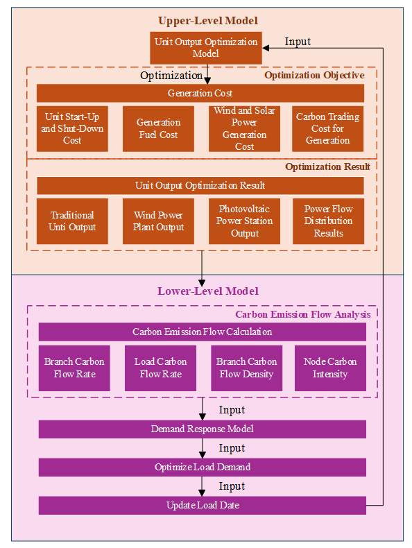
The study comprehensively incorporates source-load uncertainty and offshore user-side DR into a bi-level optimization model for marine power systems, whose overall framework is illustrated in Figure 1. The upper-level model minimizes the comprehensive operating cost, including generation cost under source-load uncertainty, unit start-up and shutdown cost, and carbon trading cost related to power generation. After solving the upper-level model, the optimized output of each generating unit and power flow distribution are obtained and then passed to the lower-level model. The lower-level model is implemented in three sequential steps:
Step 1 calculates the CEF distribution of the marine power system using the input data and CEF tracing method, and then delivers the CEF variables to Step 2.
Step 2 establishes a DR model considering DR constraints and interruptible load constraints with tiered electricity pricing suitable for the marine load side.
Step 3 solves the DR model with the objective of minimizing load cost and DR-related cost, to obtain the optimized load curve and output the adjusted load power.
Finally, the upper-level model is updated with the load data after DR implementation, thereby realizing the global coordinated optimization of the entire bi-level model for offshore wind-PV integrated marine power systems.
2.2. Two-Layer Optimization Scheduling Model for Marine Energy Systems
The proposed model consists of an upper-level model and a lower-level model. The upper-level model mainly addresses the cost optimization of generation units under uncertainty, in which the cost formulation for coal-fired power units is established based on the typical quadratic cost function [33]. The lower-level model constructs a demand response model driven by electricity price and carbon price, and the relevant demand response mechanism is formulated with reference to the mature framework [34], so as to encourage offshore load-side entities to reduce carbon emissions. The carbon emission flow theory and the corresponding calculation formulas adopted in this paper are derived from the classical research [35], which provides a solid theoretical support for the low-carbon scheduling of the model.
2.2.1. Upper-Level Model
The upper-level model considers power generation costs, carbon trading costs, and energy storage device operating costs in a comprehensive manner.
where C denotes the total operating cost of the system’s upper-level model; C1 represents the generation cost of thermal power units; C2 represents the generation cost of PV and WP; C3 represents the market carbon trading cost corresponding to unit carbon emissions; C4 represents the energy storage (ES) costs.
The generation cost of thermal power units is primarily composed of two parts: the start-up and shutdown expenses of the units, as well as the fuel consumption costs generated during the power generation process.
where aj, bj, and cj correspond to coal consumption coefficients for thermal power units; $$P_{G,j}^t$$ is the power output of unit j; Sup is start-up cost for the unit j; $$u_j^t$$ is start-up status of unit j, which takes a value of 1 or 0; NG is the set of units.
The costs associated with WP and PV power generation are primarily their operating costs:
where T denotes the total dispatch time period, set to 24 h; $$k_\mathrm{w},k_\mathrm{v}$$ stands for the unit operating cost of WP and PV power; $$\tilde{P}_\mathrm{w}^t$$ and $$\tilde{P}_\mathrm{v}^t$$ represent the WP and PV power integrated into the grid after uncertainty processing, respectively; $$P_{\mathrm{w}}^t$$ and $$P_{\mathrm{v}}^t$$ refer to the actual consumed power of WP and PV power during time t, respectively.
The market-oriented carbon trading cost for generation-side units adopts a stepped carbon emission pricing mechanism, which divides total carbon emissions into three intervals. The specific calculation formulas are as follows:
where $$\varpi$$ represents the carbon trading base price; d stands for the length of each carbon emission interval; $$M_{\mathrm{L}}^t$$ refers to the carbon emission quota allocated to the system’s generation side; $$M_{\mathrm{p}}^{t}$$ denotes the total carbon emissions within the scheduling period; $$\varepsilon_{G,j}\,$$is the CO2 emission allocation coefficient corresponding to unit electricity generation of unit j; $$\Delta\mathrm{T}$$ represents the operating duration of each thermal power unit j; $$\lambda_{G,j}$$ denotes carbon emission intensity of the unit j; τ represents the carbon price growth rate.
The comprehensive utilization cost of the ES is expressed as follows:
where Ne is the set of ES; ce stands for the unit charge-discharge cost coefficient of ES devices; $$P_{\mathrm{sc},e}^t$$ and $$P_{\mathrm{sd},e}^t$$ refers to the charging power and discharging power of ES device e at time t, respectively.
2.2.2. Upper-Level Constraints
Thermal Power Unit Operation Constraints
The constraints primarily involve their maximum output and ramping rate, which can be formulated as follows:
where $$P_{\mathrm{G},j,t}^{\min},P_{\mathrm{G},j,t}^{\max}$$ denote the minimum and maximum output limits of the thermal power unit at node j; $$r_{\mathrm{d},j}\,$$and $$r_{\mathrm{u},j}$$ represent the upper and lower bounds of the load change rate when thermal power unit j increases or decreases its output, respectively.
Renewable Energy Output Constraints
The outputs of WP and PV power need to meet the power demand constraints of each node under the scenario of insufficient unit output:
where $$P_\mathrm{w}^\mathrm{max}$$ and $$P_\mathrm{v}^\mathrm{max}$$ denote the upper limit of the output power of marine renewable energy units, respectively; $$P_\mathrm{G}^\mathrm{min}$$ represents the total minimum output of all thermal power units. Specifically, when the output of renewable energy units is insufficient, their actual outputs should comply with the power demand constraints of each node in the system.
Energy Storage Constraints
where $$S_{t}$$ denotes the ES capacity at time t; $$\theta_{i}$$ represents the energy storage loss coefficient of ES; $$\varphi_{sc,t}\,$$and $$\varphi_{sd,t}$$ represent the charging and discharging efficiency at time t, respectively; $$u_{sc,t}$$ and $$u_{sd,t}$$ indicate the charging and discharging states, respectively; $$S_{t,\min}$$ and $$S_{t,\max}$$ are the upper and lower capacity limits of ES; $$P_{sc,\max}$$ and $$P_{sd,\max}$$ represent the maximum charging and discharging power of ES, respectively.
Power Balance Constraints
In handling power balance constraints, the paper adopts the fuzzy opportunity constraint method with fuzzy variables. When dealing with uncertain variables in balance constraints, the fuzzy chance constraint method incorporating fuzzy variables is applied. When a linear relationship exists, fuzzy parameters are separated from decision variables and converted into clear equivalent classes for processing, with specific processing methods as follows:
When the confidence level is set to $$\alpha \ge 1/2$$, the clear equivalence class of $$P_r\{g(x,\zeta)\le 0\}\ge\alpha$$ is defined as follows:
where $$r_{k1}-r_{k4}\left(k=1,2,\cdots,t,t\in R\right)$$ denotes the membership function of the trapezoidal fuzzy parameter; $$h_k^+, h_k^-$$ represent two hypothetical auxiliary functions; $$h_0(x)$$ is a sub-function of $$g(x,\zeta)$$. The expression of the system’s trapezoidal fuzzy parameter is given by:
where $$\tilde{P}$$ denotes the system’s fuzzy parameter at time t; Pfore represents the predicted value of the target parameter; $$w_1 - w_4$$ is the proportional parameter, which can be derived from the historical operational data of fuzzy parameters. Thus, the system’s power balance constraints are converted into clear equivalence class forms, with triangular fuzzy parameters and clear equivalence classes applied to WP, PV power, and electrical loads:
where $$P_{\mathrm{Li}}^t, P_{\mathrm{Wi}}^t \text{ and } P_{\mathrm{Vi}}^t\,$$are the membership functions of the electrical load, WP, and PV power at time t after triangular fuzzification, respectively. The above equations illustrate that after triangular fuzzification, the node power at time t remains in a balanced state. To ensure the system possesses sufficient reserve capacity to meet the standby requirements for normal and stable operation when accounting for the output uncertainty of marine renewable energy, the following rotational reserve constraints are incorporated.
The clear equivalence class of rotational reserve is:
2.2.3. Lower-Level Model
The lower-level model is a DR optimization model, with the objective of minimizing the total load-side costs:
where F denotes the total operating cost of the lower-level model; F1 stands for the DR cost; represents the compensation cost for interruptible loads; F2 refers to the carbon emission cost.
The DR cost is computed based on the increment and decrement of the DR, as specified below:
where Nt is the total scheduling time, typically set to 24 h; $$C_{DR}$$ denotes the unit DR cost; $$DR_{\mathrm{up}}^t$$ and $$DR_{\mathrm{down}}^t$$ are the increment and decrement of DR at time t, respectively.
When the power supply is inadequate during the electricity consumption peak period, interruptible loads are temporarily curtailed or suspended in accordance with the agreements signed with the electricity department. This measure helps maintain the balance between supply and demand during peak electricity consumption periods.
where mn is the number of interruptible loads; Kint is the unit compensation cost signed by interruptible loads; $$P_{\mathrm{L,int}}$$ is the interruptible load of interruptible loads.
The carbon cost of the load-side electricity consumption is calculated using a stepped carbon price.
where $$E_{\mathrm{L,Load}}$$ denotes the carbon emission quota at time t; $$\varepsilon_L$$ stands for the unit carbon quota coefficient corresponding to load-side electricity consumption; μ is the carbon trading base price; k refers to the carbon trading price growth rate for each excess of the carbon emission interval boundary; Et is the carbon emissions generated from user-side electricity consumption at time t.
When the carbon emissions arising from marine load-side electricity consumption at time t are below the allocated carbon emission quota, the excess carbon emission quota can be traded in the carbon market to secure economic returns. The load-side adopts time-of-use (TOU) electricity pricing for electricity fee calculation. By setting differentiated electricity prices for different time periods, the marine load-side is encouraged to arrange their electricity consumption time in a reasonable manner. The electricity fee calculation formula is given as follows:
where $$C_{\text{ToU},t}$$ is the TOU electricity price at time t; $$P_{\text{mgb}}^t$$ represents the electricity consumption of the marine load-side.
2.2.4. Lower-Level Constraints
System Node Load Change Constraint
The load after DR equals the sum of the pre-response load and the load adjustment amount. Within the scheduling period D, the total system load remains unchanged before and after the implementation of DR:
where $$\beta$$ is the adjustable proportion of DR; $$P_{\mathrm{L,before}}^t$$ represents the load at time t before DR; $$P_{\mathrm{L,after}}^t$$ stands for the load at time t after DR.
Interruptible Load Constraint
The physical implications of each row in the formulas are as follows: the first row denotes the constraint on interruptible loads at each level; the second row represents the continuity constraint for interruptible loads; the third row indicates that the actual electricity consumption of the load equals the post-response load minus the interruptible load at each level.
where $$C_{\text{int},m}$$ stands for the proportion of the maximum interruptible load corresponding to the m-th level; $$P_{\ \text{L\,int},m}^t$$ denotes the variation of interruptible load for m-th level.
3. Solution Methodology
3.1. The Carbon Emission Flow Theory
The CEF calculation method acts as the core technical support throughout the bi-level optimal dispatching model of this study. Conventional approaches only assess the system’s carbon intensity through the total emissions of thermal power units, failing to quantify the carbon emissions related to load-side electricity consumption—this leads to a lack of effective basis for load-side low-carbon DR. This chapter intends to establish a comprehensive CEF calculation method covering both the source and load sides, offering technical backing for the subsequent low-carbon optimization [35].
1. The calculation formula for the carbon flow fed into the power grid by thermal power unit j within each time unit is expressed as follows:
2. By leveraging the power flow tracing technique, the carbon flow originating from generating units is distributed to individual transmission branches. The calculation formula for the branch carbon flow rate is expressed as follows:
where $$P_{G_{j,i,j}}^t$$ represents the power component flowing from thermal power unit j to branch i.
3. Node carbon potential $$NCI_i^t$$ refers to the source-side equivalent carbon emissions corresponding to unit load electricity consumption. As a core indicator linking the source and load sides, its formula is as follows:
where $$NCI_i^t$$ represent the carbon potential and original load power of node i at time t, respectively.
4. The load carbon flow rate denotes the carbon consumption of the load within each unit time, and its corresponding calculation formula is expressed as follows:
where $$P_{\text{opt},i}^t$$ is the optimized load power of node i at time t.
5. Finally, the carbon emissions of the load at time t are derived as follows:
3.2. The Source-Load Uncertainty in Marine Energy Systems
To guarantee the safe and stable operation of the power system, it is essential to maintain internal load balance and reserve adequate standby capacity. Thus, when scheduling the output of various units in the power system, both the equality balance constraints and inequality balance constraints of the system must be taken into account. At present, there are multiple approaches for researching the uncertainty prediction of WP integration and load power. However, affected by various factors, deviations exist between the predicted results and the actual power output as well as the load power. Particularly in large-scale systems with extensive WP integration, prediction deviations are non-negligible. In the day-ahead scheduling model of the power system, WP output, PV output, and load power are all regarded as uncertain variables. To analyze these uncertain variables, this study introduces fuzzy variables and converts WP output, PV output, and load power into WP fuzzy parameters, PV fuzzy parameters, and load fuzzy parameters, respectively [36].
For the stable operation of the power system, strict power equation balance constraints and rotational reserve inequality balance constraints are required. It is essential to concurrently account for the prediction deviations of the offshore WP, PV, and marine electric loads simultaneously, and their corresponding constraints can be formulated as follows:
where $$P_{\text{v}t,\text{fore}}$$ denotes the predicted value of the power load; $$\delta_{\mathrm{L}t}$$ represents the prediction error of the power load; $$P_{\text{w}t,\text{fore}}$$ is the predicted value of WP; $$P_{\text{v}t,\text{fore}}$$ stands for the predicted value of PV power; $$\delta_{\mathrm{w}t}$$ refers to the prediction error of WP; $$\delta_{\mathrm{v}t}$$ is the prediction error of PV; $$\Delta P_{_{\mathrm{w}t}}$$ is the curtailed WP in the WP dispatch plan; $$\Delta P_{_{\mathrm{v}t}}$$ is the curtailed solar power in the PV dispatch plan; nG stands for the number of conventional thermal power units; Pit denotes the output of conventional thermal power unit i; $$P_{it}^{_{\mathrm{max}}}$$ is the maximum output of conventional thermal power unit i.
In addition to the inherent output constraints of uncertain variables in the system, both the system power balance constraints and the system rotational reserve constraints involve uncertain variables. Under such circumstances, the constraints applicable under deterministic conditions will no longer be held. When scheduling the unit output in day-ahead dispatch, it is necessary to additionally consider the impact of system uncertainty. In this study, to address the uncertainties in WP, PV power, and power load, fuzzy parameters and a confidence level α are introduced to relax the power balance and rotational reserve constraints into a problem under the confidence level α. This guarantees that the probability of meeting these constraints does not fall below the predefined confidence level. On this basis, the constraints containing uncertainty are reconstructed as follows:
where $$P_r\left\{\cdot\right\}$$ denotes the occurrence likelihood of the event; α represents the preset confidence level. During the optimization process, conventional thermal power units are utilized to provide reserve capacity for the uncertainties of load, WP, and PV power. This approach considers the probability of achieving a balance between the system’s power supply and load consumption under a confidence level acceptable to decision-makers. In contrast to deterministic constraints, the system reliability opportunity constraints have already incorporated the handling of system uncertainties. Since the output of conventional thermal power units already includes reserve power, there is no need for additional reserve power configuration.
The core concept of fuzzy opportunity-constrained planning is to permit the scheduling results to not fully meet the constraints to a certain degree, while ensuring that the valid probability of the scheduling results is not lower than the pre-specified confidence level. The single-objective opportunity-constrained planning model involving fuzzy variables is formulated as follows:
where y stands for the decision variables; $$g(y, \zeta)$$ represents the objective function of the model; $$h\left(y,\zeta\right)$$ denotes constraint functions; α is the confidence level predefined by the system.
3.3. Solution Step
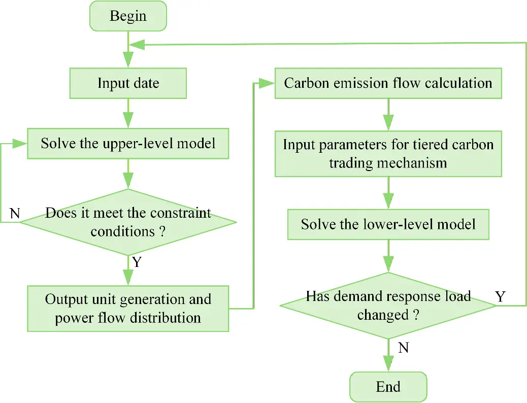
The solution steps for the proposed model in the research are depicted in Figure 2.
4. Case Study
4.1. Basic Data and Parameters
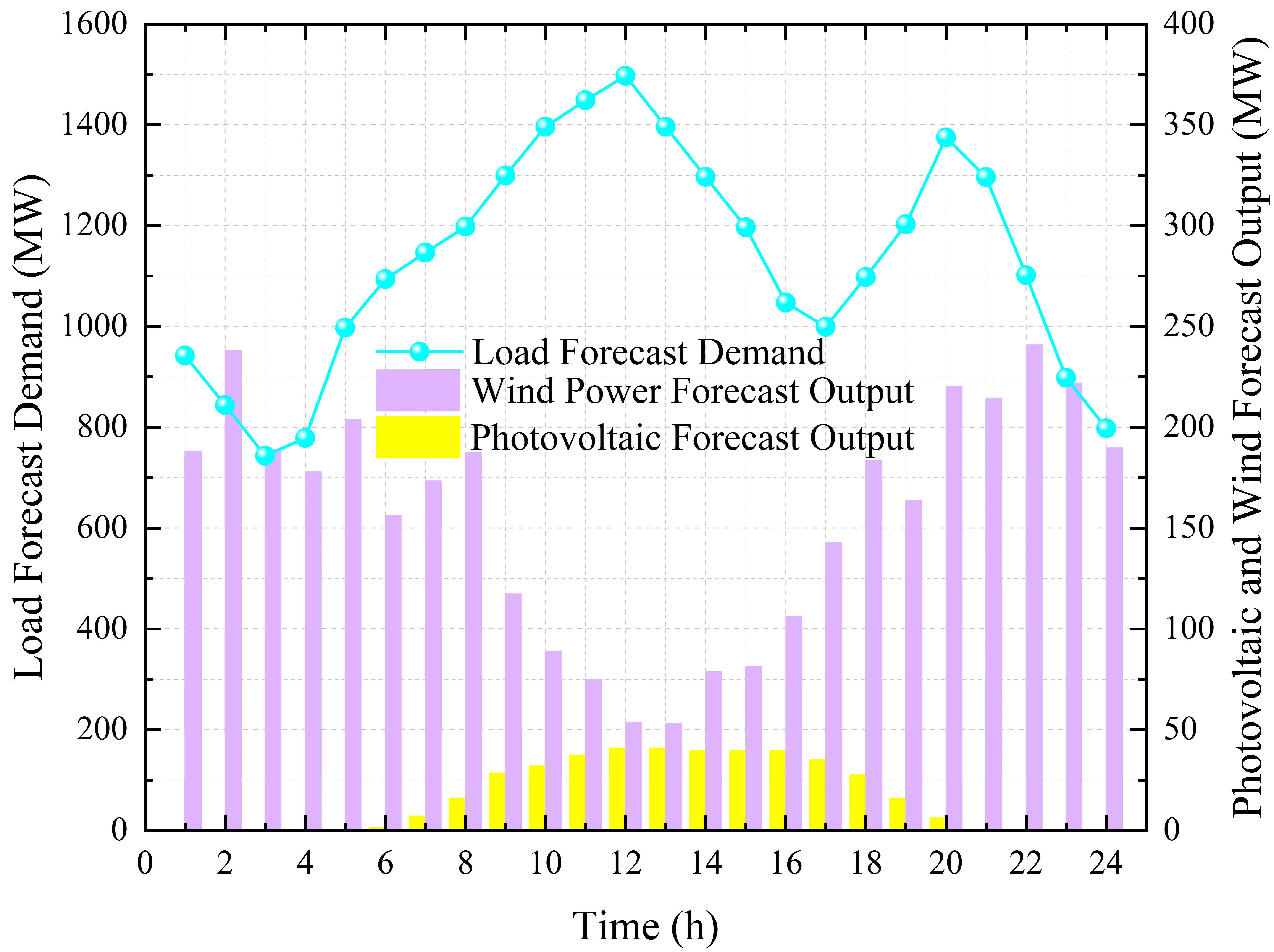
To verify the effectiveness of the proposed model, the modified IEEE 57-node system is used to emulate a typical offshore wind-PV integrated marine energy system and solve the two-stage optimization model by invoking the CPLEX solver through MATLAB. The system’s topological structure is illustrated in detail in Figure 3. The system comprises 7 generating units, which are connected to nodes 1, 2, 3, 6, 8, 9, and 12, respectively. The basic operating parameters of thermal power units are presented in Table 1 and Table 2. Nodes 9 and 12 are designated as the integration nodes for the offshore WP and PV power, with their total installed capacities being 300 MW and 50 MW, respectively. The 24-h load forecast values, WP forecast outputs, and PV power forecast outputs are depicted in Figure 4. The trapezoidal fuzzy membership parameter values corresponding to the offshore WP, PV power, and electrical load are detailed in Table 3.
In this study, the carbon emission interval length is set to 100 t, the carbon trading price growth rate is 25%, and the base carbon trading price in the carbon market is 50 yuan/t. The carbon allocation coefficient for unit electricity consumption on the load side is determined as 0.65, and the system reliability confidence level is specified as 0.9.
Table 1. Key operating parameters of thermal power units.
|
Unit |
Min Output (MW) |
Max Output (MW) |
Ramp Constraint (MW) |
Min Start-Up Time (h) |
Min Shutdown Time (h) |
Start-Up/Shutdown Cost (¥/MW) |
|---|---|---|---|---|---|---|
|
1 |
230 |
460 |
240 |
8 |
8 |
25.6 |
|
2 |
200 |
400 |
210 |
7 |
7 |
22.3 |
|
3 |
150 |
350 |
150 |
6 |
6 |
16.2 |
|
4 |
120 |
300 |
120 |
4 |
4 |
12.3 |
|
5 |
70 |
150 |
70 |
3 |
3 |
4.6 |
Table 2. Carbon emission parameters of conventional thermal power units.
|
Unit |
a (×10−5) |
b (×10−5) |
c (×10−5) |
$$\bm{{\Large \varepsilon}_{\text{G}j}}$$ (tCo2/MW) |
$$\bm{\lambda_{\boldsymbol{\mathrm{G}}_{j}}}$$ (tCo2/MW) |
|---|---|---|---|---|---|
|
1 |
1.02 |
0.277 |
9.2 |
0.877 |
0.94 |
|
2 |
1.21 |
0.288 |
8.8 |
0.877 |
0.94 |
|
3 |
2.17 |
0.29 |
7.2 |
0.877 |
0.94 |
|
4 |
3.42 |
0.292 |
5.2 |
0.877 |
0.94 |
|
5 |
6.63 |
0.306 |
3.5 |
0.979 |
1.03 |
Table 3. Trapezoidal fuzzy membership degree parameters.
|
Fuzzy Parameter Object |
$$\bm{w_1}$$ | $$\bm{w_2}$$ | $$\bm{w_3}$$ |
|---|---|---|---|
|
WP |
0.6 |
1 |
1.4 |
|
PV output |
0.5 |
1 |
1.5 |
|
Load |
0.9 |
1 |
1.1 |
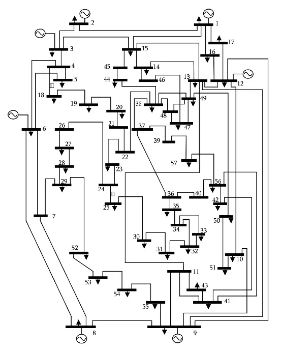
Figure 3. IEEE 57-bus electrical wiring diagram. Note: Numbers (1–57) denote bus IDs; downward-pointing arrows represent load buses; the “II” mark is a graphical indicator for double-line transmission branches and has no specific physical implication.
4.2. Analysis of Power Dispatch Results
To verify the effectiveness of the optimized dispatch model integrating CEF theory, fuzzy opportunity constraints, and the DR model, three analytical scenarios are designed to cover safety-oriented, economy-oriented, and comprehensive optimization of safety, economy, and environmental protection. The specific settings are as follows:
Scenario 1: The upper-level model adopts a fuzzy opportunity constraint approach to address the uncertainties of the offshore WP, PV output, and load of the marine energy system. The lower-level model does not incorporate the DR mechanism, focusing solely on the operational optimization of source-side units without load-side flexible adjustment.
Scenario 2: The upper-level model employs deterministic constraints on the system’s power balance requirements. To cope with the uncertainties of the offshore WP, PV output, and load forecasting, the system’s rotational reserve capacity is set to 20% of the total grid-connected capacity of renewable energy, and the electrical load forecast value is adjusted to 90% of the original load forecast value. The lower-level model introduces the constructed DR model to realize load-side flexibility regulation.
Scenario 3: The upper-level model uses a fuzzy opportunity constraint model to address uncertainty issues. The DR model is introduced in the lower-level model.
The total operating costs, total carbon emissions, and total reserve capacity under different scenarios are presented in Table 4. Scenario 3 employs the bi-level low-carbon dispatch model proposed in this paper, which features the lowest carbon emissions and the optimal comprehensive operating costs. Compared with Scenario 1, the proposed model reduces carbon emissions by 16.05% and comprehensive operating costs by 15.75%. Meanwhile, the total reserve capacity decreases by 387.3 MW during the same dispatch cycle. This improvement arises because Scenario 1 does not involve load-side DR, thus requiring extra reserve capacity to ensure the safe and stable operation of the marine power system during peak load periods. The comparison between Scenario 1 and 3 demonstrates that DR implementation encourages offshore load-side adoption of low-carbon power consumption patterns, effectively reducing carbon emissions, comprehensive operating costs, and the reserve capacity requirements of generation units.
Table 4. Operational comparison of different scenarios.
|
Scenario |
Total Carbon Emissions (tons) |
Total Operating Cost (×104 yuan) |
Total Reserve Capacity (MW) |
|---|---|---|---|
|
1 |
47,349.68 |
1414.80 |
3120.2 |
|
2 |
41,341.23 |
1211.69 |
2517.4 |
|
3 |
39,653.93 |
1192.00 |
2732.9 |
Compared with Scenario 2, Scenario 3 reduces carbon emissions by approximately 4.08% and comprehensive operating costs by about 1.63%, which confirms its superior low-carbon and economic performance. However, the total reserve capacity of units increases by 215.5 MW. The main reason is that Scenario 2 adopts deterministic power balance constraints, which ignore the forecasting errors of offshore WP, offshore PV output, and marine electrical loads. Accordingly, power generation can be scheduled only according to the preset forecasting scheme without high reserve capacity. In contrast, Scenario 3 adopts the fuzzy chance-constrained model, which considers power balance under a specified confidence level to guarantee the operational security of the marine power system. Therefore, the dispatch strategy is more consistent with the practical operation characteristics of offshore renewable-integrated marine energy systems.
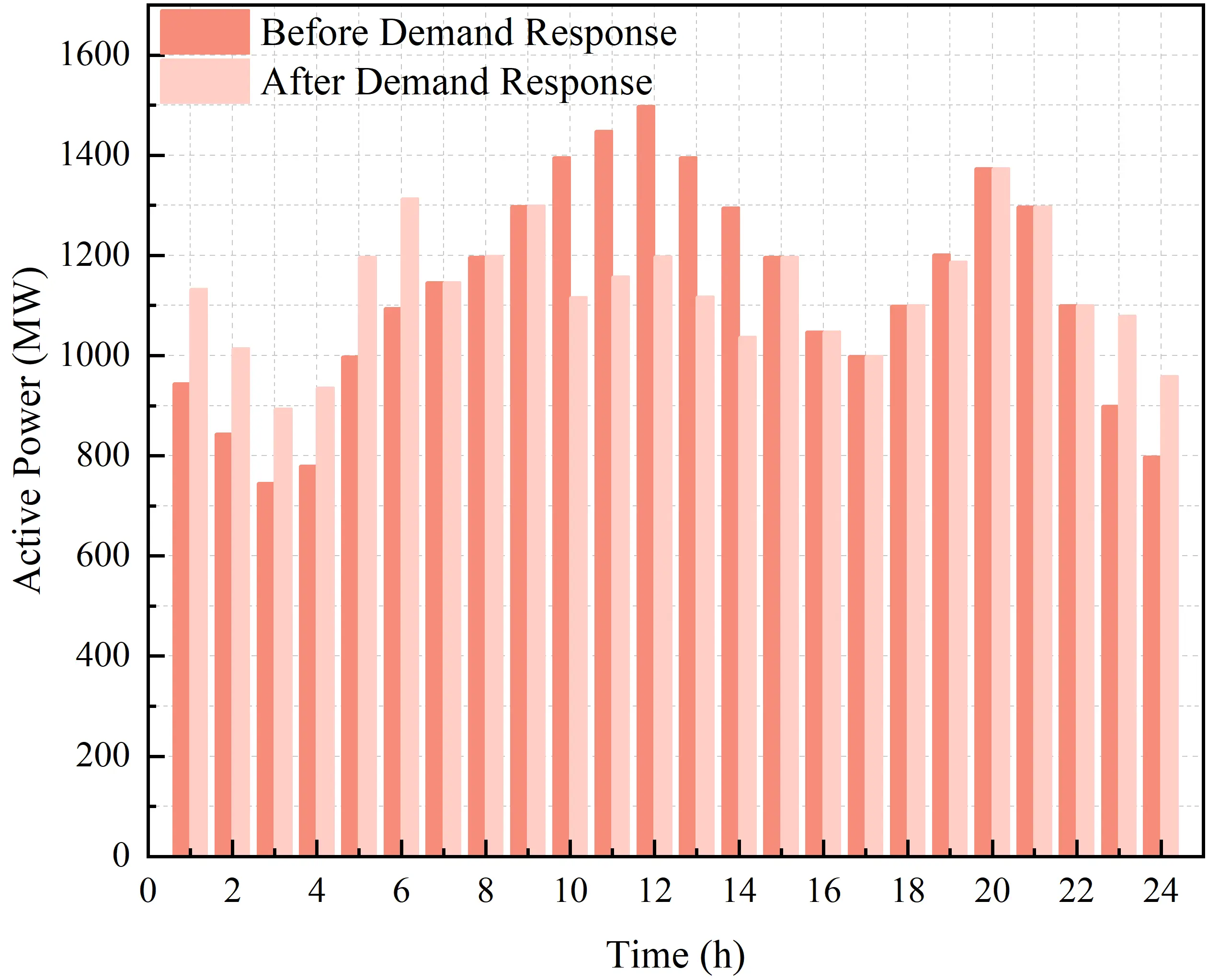
The load variations before and after the implementation of DR are depicted in Figure 5. During the peak electricity consumption period (9:00–15:00), the marine electrical load shows a remarkable reduction after the DR mechanism is applied. By contrast, during off-peak periods (1:00–6:00 and 23:00–24:00), the load increases slightly, contributing to a more balanced load distribution across the marine power grid. This phenomenon can be explained as follows: during peak hours, the power supply capacity of the offshore system is relatively tight. Users with interruptible load qualifications voluntarily reduce or suspend their power consumption in accordance with agreements signed with the grid operator, which effectively relieves the load pressure of the marine system during peak periods. Users can shift part of their transferable load to off-peak hours and take advantage of the TOU pricing policy to lower their electricity costs. During off-peak hours, the lower electricity prices motivate users to increase power consumption, thus improving the utilization efficiency of marine renewable energy resources. From an energy management perspective, offshore load-side DR enables peak shaving and valley filling of electrical loads in marine systems. Through flexible load regulation, the overall operational efficiency of the marine power system is enhanced, reducing both generation costs and grid losses while keeping the total electrical load unchanged.
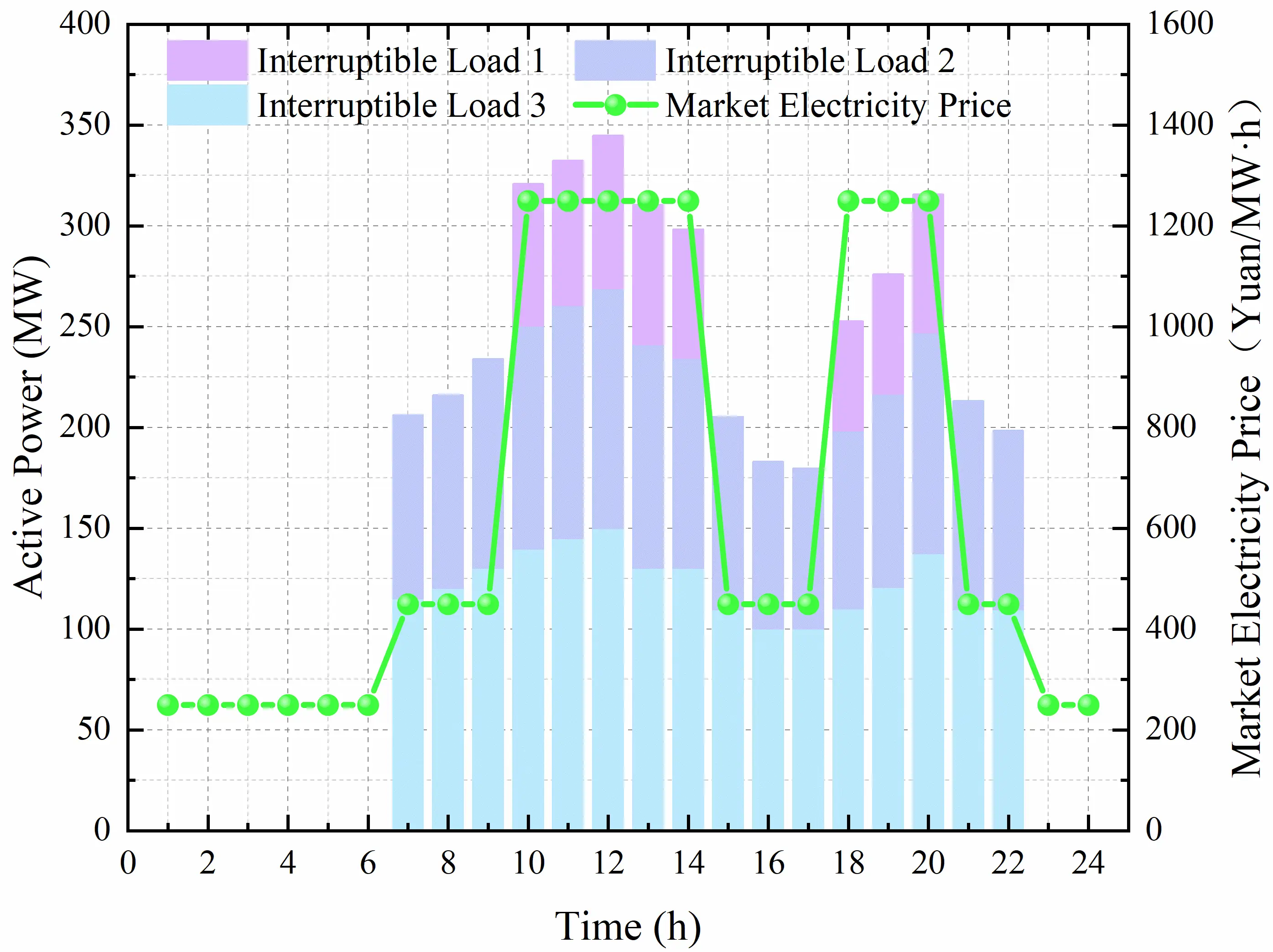
The dispatch results over one dispatch cycle after the implementation of interruptible load agreements are illustrated in Figure 6. The figure shows the 24 h active power variations of three level interruptible loads and the fluctuation trend of market electricity prices in the marine power system. The active power response of each interruptible load level differs considerably across periods. Nevertheless, during hours with high electricity prices, the active power adjustment of these loads clearly reflects a rational response to economic incentives.
Each level of interruptible load responds dynamically to TOU electricity price changes. Specifically, whether evaluated individually or in terms of their overall superposition, the active power of interruptible loads rises with increasing electricity prices and falls with decreasing prices. This achieves precise coordination among load interruption, system operational demand, and economic incentives. Offshore users can strategically participate in demand-side response to reduce electricity costs during peak periods, while the marine power grid effectively relieves peak operational pressure.
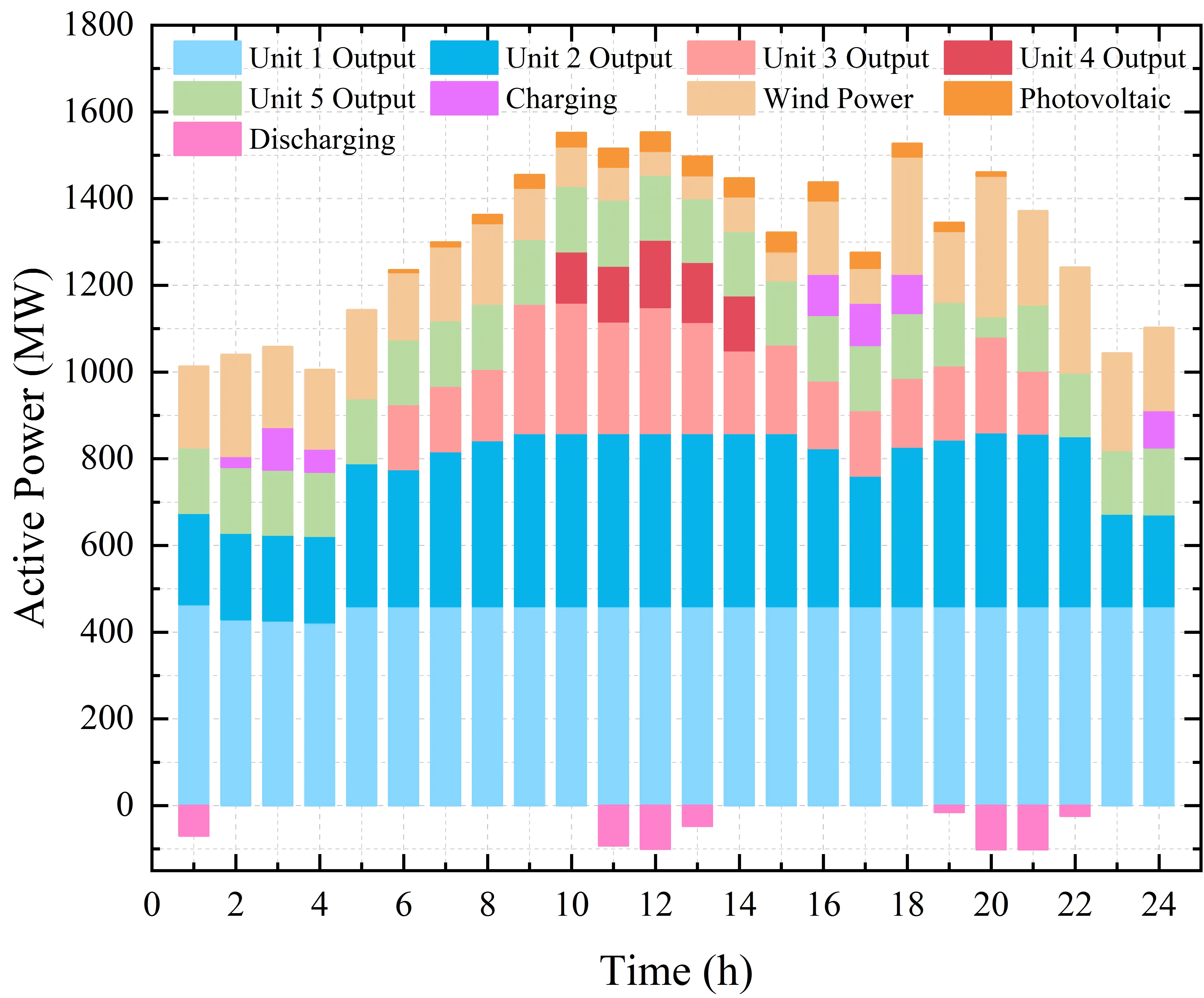
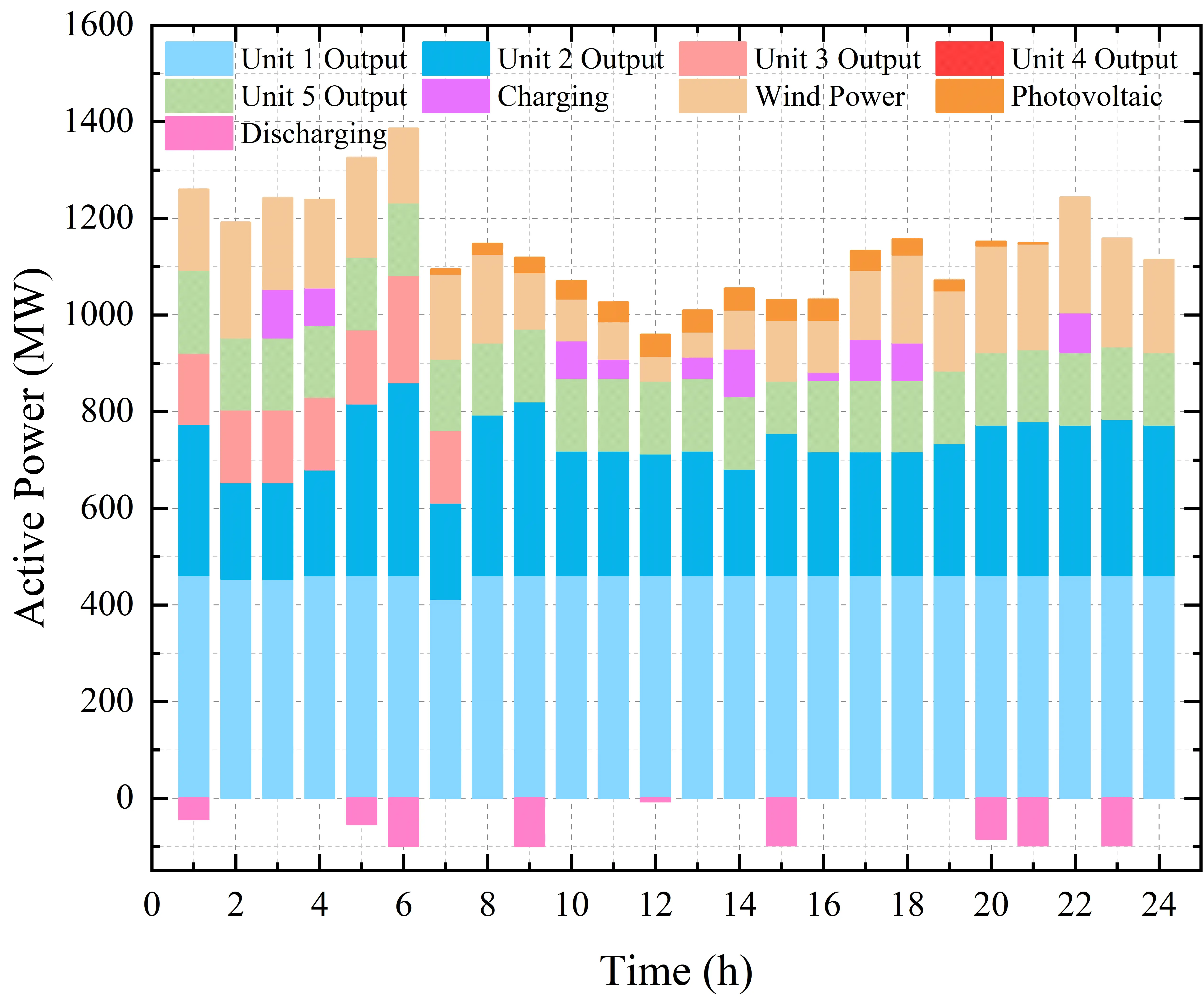
Both Scenario 1 and Scenario 3 adopt the fuzzy chance-constrained model, where the output of each generating unit satisfies the power balance under a 0.9 confidence level, meeting the expected requirements of decision-makers for marine power system operation. The unit outputs before and after optimization are illustrated in Figure 7. As shown in Figure 7a, during the peak electricity consumption period (9:00–15:00) prior to optimization, the outputs of conventional thermal power units 2, 3, and 4 increased significantly to meet the marine load demand. However, thermal power generation is associated with substantial carbon emissions, hindering the low-carbon, sustainable development of marine energy systems. Offshore renewable energy units (offshore wind and PV) exhibit large output fluctuations due to the variability of marine natural conditions, and their intermittency poses challenges to a stable power supply during peak load periods. Although energy storage devices can regulate the balance between power supply and consumption by charging during off-peak periods and discharging during peak periods, their adjustment capability is limited by capacity and efficiency constraints in marine scenarios.
Figure 7b demonstrates significant changes in the output distribution of generating units after optimization. The DR strategy effectively achieved peak shaving for peak-period marine loads, alleviating the power generation pressure on units during peak hours. During the 10:00–14:00 window, the original marine load demand required units 1, 2, and 3 to operate at full load, with units 4 and 5 running at high efficiency. After optimization, unit 1 still needs to operate at full load, while units 2 and 5 can meet the load demand with lower output levels. Additionally, the output of each thermal power unit becomes more stable across different time periods, ensuring the operational stability of the marine power system, reducing unit maintenance costs, and extending the service life of power generation equipment. Meanwhile, as DR optimizes the marine load curve, offshore renewable energy units can participate in power supply more effectively throughout the day, increasing the proportion of renewable energy generation in the marine power system. In summary, the adoption of the DR model results in a smoother system load curve, reducing the output of thermal power units during peak periods and facilitating better absorption of offshore renewable energy output.
 |
 |
|
(a) |
(b) |
Figure 7. Generator output before and after optimization. (a) Before optimization; (b) after optimization.
4.3. Carbon Emission Scheduling Results Analysis
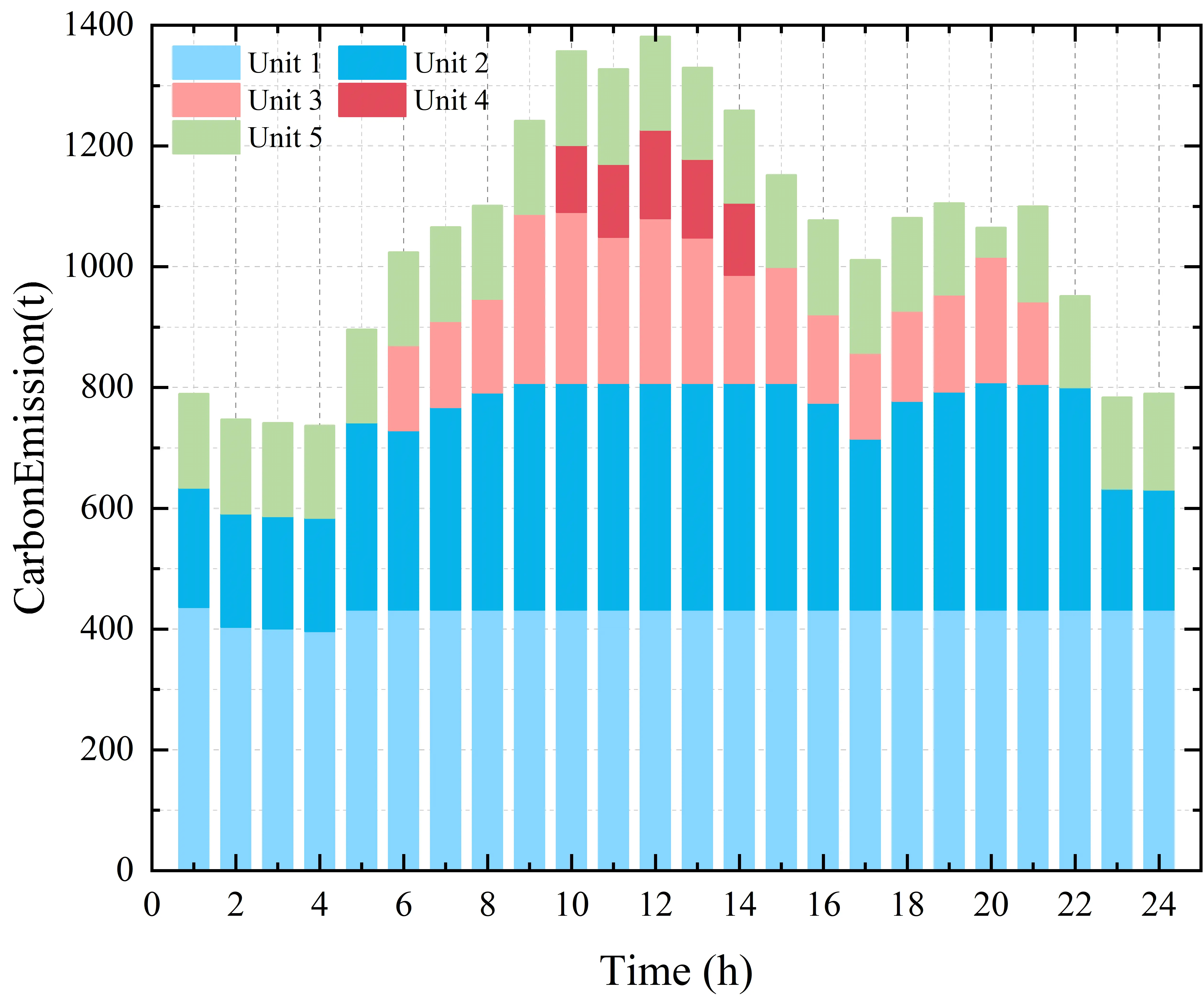
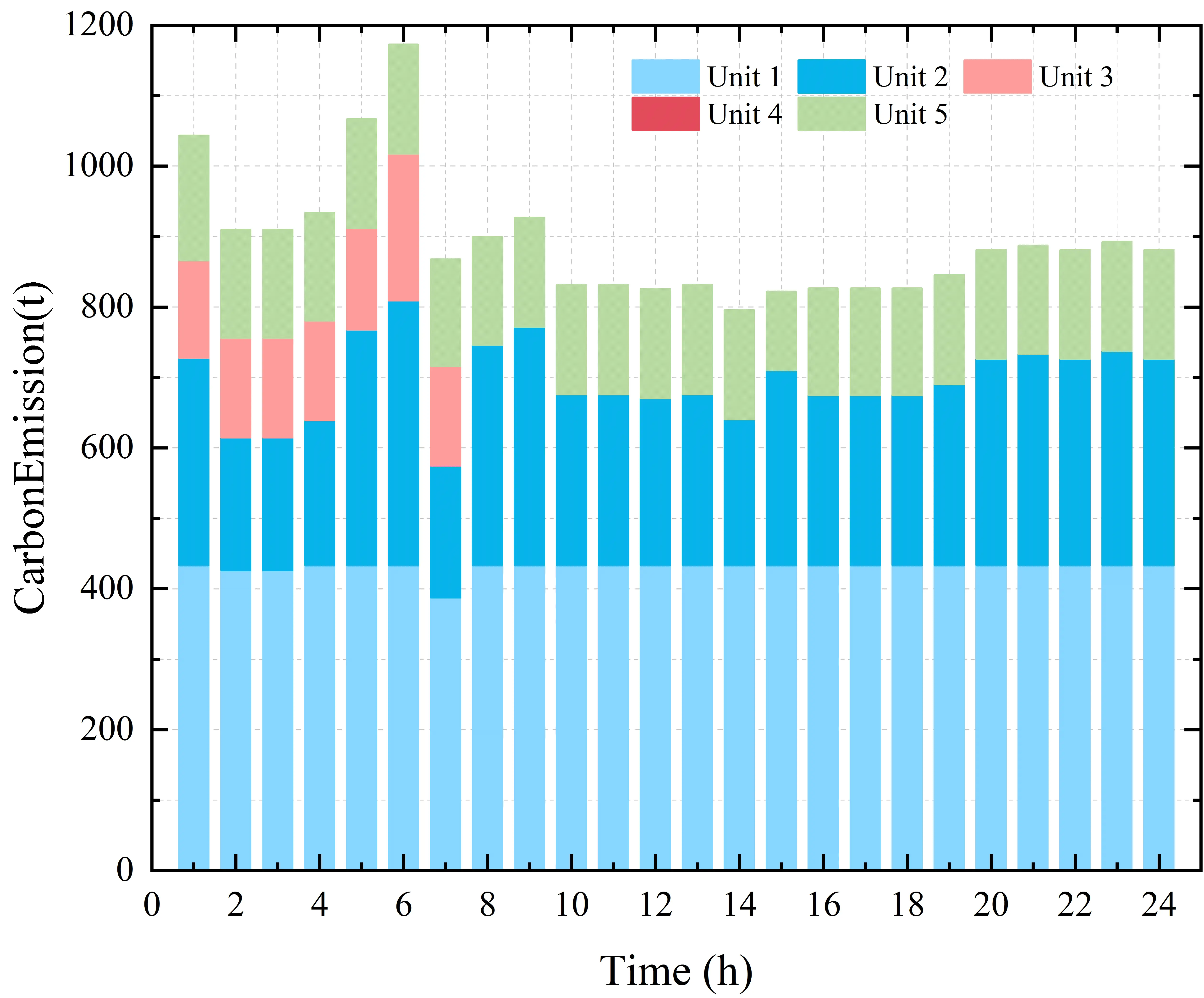
4.3.1. Analysis of Carbon Emissions from Power Generation
Within the dispatch cycle, the carbon emissions of each generating unit before and after optimization are illustrated in Figure 8. After optimization, the carbon emissions of the entire marine power generation system show a significant reduction, decreasing by approximately 16.5% within the same dispatch cycle. This reduction is primarily attributed to the effective mitigation of offshore users’ peak-period load and the improved absorption rate of offshore WP and PV power in the marine system. Additionally, during peak electricity consumption periods, measures such as interruptible load response reduce the system’s power generation demand, avoiding the need for generating units to operate at full load and thereby cutting down fossil fuel consumption and carbon dioxide emissions in marine power systems.
 |
 |
|
(a) |
(b) |
Figure 8. Carbon emissions of thermal power units before and after optimization. (a) Before optimization; (b) after optimization.
As shown in Figure 8b, the carbon emissions of each generating unit vary relatively moderately during off-peak periods. This indicates that while DR effectively reduces carbon emissions during peak periods, it does not exert a negative impact on power supply stability and carbon emission levels during off-peak periods of the marine system. The optimized carbon emission curve is more stable, reflecting that under the regulation of DR, the carbon emissions of the marine power system are more consistent and predictable, which is conducive to the low-carbon management and stable operation of offshore renewable-integrated energy systems.
4.3.2. Analysis of Carbon Emissions from the User Side
Based on the optimal dispatch results at the upper level, load-side carbon emissions are calculated using CEF theory. The load-side carbon emissions before and after DR, as well as the carbon emission characteristics under interruptible load dispatch, are illustrated in Figure 9. As shown in the figure, the reduction in load demand effectively suppresses load-side carbon emissions, especially during peak electricity consumption periods. Combined with Table 5, it can be concluded that the total load-side carbon emissions of the marine power system decrease over the entire dispatch cycle. After implementing interruptible load dispatch, the load-side carbon emission cost is reduced by 2.86%, and the total carbon emissions are decreased by 17.65% within one dispatch cycle, respectively.
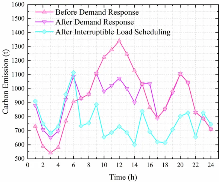
Table 5. Comparison before and after demand response.
|
Before and After Response |
Total Load-Side Carbon Emissions (tons) |
Total Load-Side Carbon Emissions Cost (yuan) |
|---|---|---|
|
Before response |
22,123.4 |
220,466 |
|
After response |
21,941.2 |
214,153 |
|
After interruptible load dispatch |
18,218.3 |
174,161 |
It is evident that interruptible load response can effectively relieve the electricity supply pressure of the marine system, while significantly reducing the total carbon emissions and carbon-related costs on the offshore load side. The above analysis demonstrates that compensation for interruptible loads and the corresponding reduction in power demand have a remarkable effect on lowering system carbon emissions, which verifies the rationality and effectiveness of the proposed bi-level low-carbon optimal dispatch model for offshore wind-PV integrated marine energy systems.
In summary, demand response and interruptible load dispatch can not only effectively reduce carbon emissions during peak periods but also enhance the stability of load-side carbon emissions, thereby promoting more efficient, low-carbon operation of the entire marine power system.
4.4. Impact Analysis of Confidence Level in Fuzzy Chance-Constrained Programming
To verify the robustness of the proposed fuzzy chance-constrained model and the rationality of parameter selection, sensitivity analysis is carried out under four typical confidence levels: α = 0.8, 0.85, 0.9, and 0.95. The effects of the confidence level on three key system indices, namely total operating cost, total carbon emissions, and total reserve capacity, are investigated in detail to provide a scientific basis for determining the confidence level used in the paper.
As shown in Table 6, with the increase of the confidence level, the system operating cost and reserve capacity increase gradually, while the carbon emissions decrease slightly and tend to be stable. The reserve capacity is the most sensitive to the confidence level and shows approximately linear growth. Carbon emissions are mainly dominated by carbon trading, carbon emission flow tracing, and demand response, and are barely affected by the confidence level, reflecting the strong robustness of the proposed low-carbon dispatch framework. In terms of variation trend, the growth rates of total operating cost and total reserve capacity from 0.9 to 0.95 are significantly higher than those from 0.8 to 0.9. The comprehensive analysis demonstrates that α = 0.9 achieves the optimal balance among operational economy, carbon emission reduction, and reserve capacity allocation. It not only meets the security constraints of offshore power systems under source-load uncertainty but also avoids excessive cost and reserve waste caused by over-conservatism, showing good engineering practicability.
Table 6. Comparison of different confidence levels.
|
α |
Total Operating Cost (×104 yuan) |
Total Carbon Emissions (tons) |
Total Reserve Capacity (MW) |
|---|---|---|---|
|
0.80 |
1168.5 |
39,981.2 |
2415.1 |
|
0.85 |
1179.3 |
39,762.5 |
2578.6 |
|
0.90 |
1192.0 |
39,653.9 |
2732.9 |
|
0.95 |
1215.7 |
39,610.3 |
2964.2 |
5. Conclusions
This paper proposes a bi-level low-carbon economic dispatch model for offshore wind-PV grid-connected marine power systems that fully considers source-load uncertainty and carbon emission flow. The upper layer addresses the randomness and volatility of offshore renewable energy and marine loads using trapezoidal fuzzy parameters and fuzzy chance-constrained programming, to realize the economic and low-carbon output optimization of generating units. The lower layer constructs a low-carbon demand response model driven by carbon price signals and CEF-based node carbon quantification, achieving coordinated optimization of generation-side economy and load-side emission reduction. Based on the modified IEEE 57-node system and CPLEX solver, the effectiveness and advancement of the proposed model are verified. The main conclusions are drawn as follows:
- (a)
-
The trapezoidal fuzzy parameter method can effectively address source-load uncertainty under large-scale offshore wind and PV grid integration. By optimizing the output of thermal power units through fuzzy chance constraints under a preset confidence level, the method ensures system operational security while reducing reserve capacity and overall operating costs of marine power systems
- (b)
-
Integrating CEF theory with a stepwise carbon trading mechanism enables accurate allocation of generation-side carbon emissions to the load side. This allows direct quantification of offshore user-side carbon emissions and effective transmission of carbon price signals. Numerical results show that this scheme brings a 17.65% reduction in load-side carbon emissions and a 21% decrease in carbon-related costs, which significantly improves the low-carbon performance of the marine power system.
- (c)
-
The proposed bi-level optimal dispatching model, with CEF as the coupling link, achieves significant performance improvements. Case studies comparing three scenarios demonstrate that the model reduces total system carbon emissions by 16.05% and comprehensive operating costs by 15.75%. It realizes the coordinated optimization of safety, economy, and environmental friendliness for marine power systems with large-scale offshore renewable integration, providing a feasible technical pathway for the low-carbon transition of marine energy systems.
6. Research Limitations and Future Research Directions
Despite the effectiveness and superiority of the proposed method demonstrated via simulations on the IEEE 57-node test system, this study still has limitations that deserve further investigation. First, the simulation validation is limited to a standard test system rather than a practical, large scale power grid. Although the proposed model and framework are modular and theoretically scalable, their performance under actual grid topology, real world operation data, and complex operational rules still needs to be verified in engineering practice. Second, computational performance under large scale scenarios with massive variables and constraints is not fully tested, and more efficient solving strategies such as decomposition methods or parallel computing deserve to be explored to improve computational efficiency. Third, this study focuses on day ahead scheduling, and more real time operation constraints, communication delays, and dynamic adjustment mechanisms can be further considered to enhance the practicality of the proposed method. Future work will extend the proposed method to practical large scale offshore wind PV integrated power systems and combine advanced optimization techniques to promote engineering application.
Author Contributions
Q.G.: Writing—review & editing, Project administration, Formal analysis. L.G.: Writing—review & editing, Writing—original draft, Visualization, Software, Methodology. Z.M.: Writing—review & editing, Resources, Data curation. Q.C.: Writing—review & editing, Data curation. S.S.: Writing—review & editing, Supervision, Methodology. J.L.: Writing—review & editing, Methodology, Visualization, Software. Y.J.: Writing—review & editing, Methodology.
Ethics Statement
Not applicable for studies not involving humans or animals.
Informed Consent Statement
Not applicable for studies not involving humans.
Data Availability Statement
Data will be made available on request.
Funding
This work was supported by the Natural Science Foundation of Tianjin (No. 24JCYBJC00280).
Declaration of Competing Interest
The authors declare that they have no known competing financial interests or personal relationships that could have appeared to influence the work reported in this paper.
References
- Toms AM, Li X, Rajashekara K. Optimal microgrid sizing of offshore renewable energy sources for offshore platforms and coastal communities. Sustain. Energy Grids Netw. 2025, 44, 101989. DOI:10.1016/j.segan.2025.101989 [Google Scholar]
- Ma X, Li M, Li W, Liu Y. Overview of offshore wind power technologies. Sustainability 2025, 17, 596. DOI:10.3390/su17020596 [Google Scholar]
- Pizzuti I, Magni GU, Delibra G, Garcia DA, Corsini A. Integrating desalination in Renewable Energy Communities: A study on Ventotene island. Renew. Energy 2025, 254, 123759. DOI:10.1016/j.renene.2025.123759 [Google Scholar]
- Li Y, Yang X, Du E, Liu Y, Zhang S, Yang C, et al. A review on carbon emission accounting approaches for the electricity power industry. Appl. Energy 2024, 359, 122681. DOI:10.1016/j.apenergy.2024.122681 [Google Scholar]
- Zhang Y, Yuan C, Du X, Chen T, Hu Q, Wang Z, et al. Capacity configuration of hybrid energy storage system for ocean renewables. J. Energy Storage 2025, 116, 116090. DOI:10.1016/j.est.2025.116090 [Google Scholar]
- Mugambi GR, Darii N, Khazraj H, Saborío-Romano O, Raducu AG, Sharma R, et al. Methodologies for offshore wind power plant dynamic stability analysis. Renew. Sustain. Energy Rev. 2025, 216, 115635. DOI:10.1016/j.rser.2025.115635 [Google Scholar]
- Saleem MI, Saha S. Assessment of frequency stability and required inertial support for power grids with high penetration of renewable energy sources. Electr. Power Syst. Res. 2024, 229, 110184. DOI:10.1016/j.epsr.2024.110184 [Google Scholar]
- Ouyang T, Li Y, Xie S, Wang C, Mo C. Low-carbon economic dispatch strategy for integrated power system based on the substitution effect of carbon tax and carbon trading. Energy 2024, 294, 130960. DOI:10.1016/j.energy.2024.130960 [Google Scholar]
- Lari DS, Nafar M, Abbasi AR, Bahmani-Firouzi B. Probabilistic scheduling of microgrid resilience: Integrating renewables, storages and demand response in unit commitment and reconfiguration. Int. J. Electr. Power Energy Syst. 2025, 168, 110710. DOI:10.1016/j.ijepes.2025.110710 [Google Scholar]
- Ahmed MMR, Mirsaeidi S, Koondhar MA, Karami N, Tag-Eldin EM, Ghamry NA, et al. Mitigating uncertainty problems of renewable energy resources through efficient integration of hybrid solar PV/wind systems into power networks. IEEE Access 2024, 12, 30311–30328. DOI:10.1109/ACCESS.2024.3370163 [Google Scholar]
- Taraghi Nazloo H, Babazadeh R, Varmazyar M. Optimal Configuration and Planning of Distributed Energy Systems Considering Renewable Energy Resources. J. Environ. Inform. 2024, 43, 50–64. DOI:10.3808/jei.202400508 [Google Scholar]
- Ji Y, An A, Zhang L, He P, Liu X. Short-term load forecasting based on temporal importance analysis and feature extraction. Electr. Power Syst. Res. 2025, 244, 111551. DOI:10.1016/j.epsr.2025.111551 [Google Scholar]
- Du SY, Tan DH, Chen Z. Optimization and scheduling of combined heat and power system considering wind power uncertainty and demand response. COMPEL 2025, 44, 248–267. DOI:10.1108/COMPEL-05-2024-0227 [Google Scholar]
- Cao Z, Wang J, Xia Y. Combined electricity load-forecasting system based on weighted fuzzy time series and deep neural networks. Eng. Appl. Artif. Intell. 2024, 132, 108375. DOI:10.1016/j.engappai.2024.108375 [Google Scholar]
- Aljeddani SM, Mohammed MA. An extensive mathematical approach for wind speed evaluation using inverse Weibull distribution. Alexandria Eng. J. 2023, 76, 775–786. DOI:10.1016/j.aej.2023.06.076 [Google Scholar]
- Kumar A, Mishra B. Nonlinear fuzzy chance constrained approach for multi-objective mixed fuzzy-stochastic optimization problem. OPSEARCH 2024, 61, 121–136. DOI:10.1007/s12597-023-00699-0 [Google Scholar]
- Zhang J, Zhang Z, Cai X, Cai J, Chen J. An interval evolutionary algorithm based on dynamic relation adjustment strategy for many-objective problems. Swarm Evol. Comput. 2025, 93, 101853. DOI:10.1016/j.swevo.2025.101853 [Google Scholar]
- Tong X, Zhao S, Chen H, Wang X, Liu W, Sun Y, et al. Optimal dispatch of a multi-energy complementary system containing energy storage considering the trading of carbon emission and green certificate in China. Energy 2025, 314, 134215. DOI:10.1016/j.energy.2024.134215 [Google Scholar]
- Tong X, Zhao S, Chen H, Wang X, Liu W, Sun Y, et al. Comprehensive carbon accounting for power systems considering hybrid power trading mode. Energy 2025, 333, 136897. DOI:10.1016/j.energy.2025.136897 [Google Scholar]
- Zheng L, Zhou B, Chung CY, Li J, Cao Y, Zhao Y. Coordinated operation of multienergy systems with uncertainty couplings in electricity and carbon markets. IEEE Internet Things J. 2024, 11, 24414–24427. DOI:10.1109/JIOT.2024.3355132 [Google Scholar]
- Song X, Wu H, Zhang J, Zhao C, Peña-Mora F. Optimal operation of shared energy storage-assisted wind-solar-thermal power generation systems under the electricity-carbon markets. Energy 2025, 330, 136614. DOI:10.1016/j.energy.2025.136614 [Google Scholar]
- Faria WR, Muñoz-Delgado G, Contreras J, Pereira Junior BR. Distribution and transmission coordinated dispatch under joint electricity and carbon day-ahead markets. Sustain. Energy Grids Netw. 2024, 38, 101393. DOI:10.1016/j.segan.2024.101393 [Google Scholar]
- Zhai Z, Zhang L, Wang Y, Hou X, Yang Q. Optimization of power generation structure and electricity transmission pattern in China based on the electricity-carbon coordinated market. Renew. Energy 2025, 252, 123359. DOI:10.1016/j.renene.2025.123359 [Google Scholar]
- Zhang J, Liu Z. Low carbon economic scheduling model for a park integrated energy system considering integrated demand response, ladder-type carbon trading and fine utilization of hydrogen. Energy 2024, 290, 130311. DOI:10.1016/j.energy.2024.130311 [Google Scholar]
- Sun X, Bao M, Ding Y, Hui H, Song Y, Zheng C, et al. Modeling and evaluation of probabilistic carbon emission flow for power systems considering load and renewable energy uncertainties. Energy 2024, 296, 130768. DOI:10.1016/j.energy.2024.130768 [Google Scholar]
- Liang H, Pirouzi S. Energy management system based on economic Flexi-reliable operation for the smart distribution network including integrated energy system of hydrogen storage and renewable sources. Energy 2024, 293, 130745. DOI:10.1016/j.energy.2024.130745 [Google Scholar]
- Pandya SB, Kalita K, Jangir P, Cep R, Migdady H, Chohan JS, et al. Multi-objective RIME algorithm-based techno economic analysis for security constraints load dispatch and power flow including uncertainties model of hybrid power systems. Energy Rep. 2024, 11, 4423–4451. DOI:10.1016/j.egyr.2024.04.016 [Google Scholar]
- Song Y, Mu H, Li N, Wang H, Kong X. Optimal scheduling of zero-carbon integrated energy system considering long-and short-term energy storages, demand response, and uncertainty. J. Clean. Prod. 2024, 435, 140393. DOI:10.1016/j.jclepro.2023.140393 [Google Scholar]
- Wang L, Lin J, Dong H, Wang Y, Zeng M. Demand response comprehensive incentive mechanism-based multi-time scale optimization scheduling for park integrated energy system. Energy 2023, 270, 126893. DOI:10.1016/j.energy.2023.126893 [Google Scholar]
- Li P, Li Y, Li Z, Jia Q. Multi-time scale game dispatching strategy for microgrid cluster with shared energy storage considering demand response uncertainty. Energy 2025, 328, 136568. DOI:10.1016/j.energy.2025.136568 [Google Scholar]
- Zhan H, Qin Y, Xiong X, Qi H, Hu J, Tang J, et al. A Dual-Layer Optimal Operation of Multi-Energy Complementary System Considering the Minimum Inertia Constraint. Energies 2025, 18, 5202. DOI:10.3390/en18195202 [Google Scholar]
- Amouzadrad P, Mohapatra SC, Guedes Soares C. Review on Sensitivity and Uncertainty Analysis of Hydrodynamic and Hydroelastic Responses of Floating Offshore Structures. J. Mar. Sci. Eng. 2025, 13, 1015. DOI:10.3390/jmse13061015 [Google Scholar]
- Yuan X, Chen H, Yu T, Zheng H, Pan P, Wang X, et al. Optimal dispatch of coal-fired power units with carbon capture considering peak shaving and ladder-type carbon trading. Energy 2024, 313, 133803. DOI:10.1016/j.energy.2024.133803 [Google Scholar]
- Li P, Ni Z, Lei X, Ye K, Han Z. Low carbon optimal dispatch of integrated energy systems considering V2G and demand response under carbon trading mechanisms. Sustain. Energy Fuels 2025, 9, 6216–6234. DOI:10.1039/D5SE01008J [Google Scholar]
- Li P, Ni Z, Lei X, Ye K, Han Z. Low-carbon optimal learning scheduling of the power system based on carbon capture system and carbon emission flow theory. Electr. Power Syst. Res. 2023, 218, 109215. DOI:10.1016/j.epsr.2023.109215 [Google Scholar]
- Zhang S, Hu W, Cao X, Du J, Zhao Y, Bai C, et al. A two-stage robust low-carbon operation strategy for interconnected distributed energy systems considering source-load uncertainty. Appl. Energy 2024, 368, 123457. DOI:10.1016/j.apenergy.2024.123457 [Google Scholar]