
An Investment Framework for Multi-Energy Complementary System Based on the Pythagorean Fuzzy Prospect-GLDS Model

An Investment Framework for Multi-Energy Complementary System Based on the Pythagorean Fuzzy Prospect-GLDS Model

Received: 16 January 2026 Revised: 17 March 2026 Accepted: 10 April 2026 Published: 07 May 2026

© 2026 The authors. This is an open access article under the Creative Commons Attribution 4.0 International License (https://creativecommons.org/licenses/by/4.0/).
1. Introduction
Against the backdrop of significant shifts in the worldwide energy landscape and the rapid advancement of the “dual carbon” objectives, traditional energy supply models encounter numerous challenges, including resource shortages, environmental pollution, and unstable supply, making it difficult to meet the increasing and diverse energy demands of modern society [1]. MECS, with its ability to integrate various energy forms such as wind, solar, hydro, storage, and hydrogen into a collaborative optimization system, has become the core solution to address the energy trilemma. As an important form of decentralized energy distribution, microgrids are the key carrier of MECS, and recent studies have systematically reviewed the advancements in microgrid planning and optimization for renewable energy integration [2], which provides a theoretical basis for the construction of the MECS investment decision-making framework in this paper. By coordinating the spatiotemporal complementary characteristics of different energy sources, MECS can significantly enhance energy efficiency, smooth fluctuations in renewable energy, and reduce environmental impact [3,4]. For example, the multi-interconnected integrated energy system optimization model proposed by Wang reduces the system’s energy purchase cost by 1.48% and increases the operator’s profit by 30.41% through an adaptive pricing system and a collective demand response approach [3]. Additionally, the practical example of the China National Nuclear Corporation’s Deha solar thermal storage integrated project in Qinghai Province (equipped with 800 MW of photovoltaic power, 200 MW of solar thermal storage, and an energy storage system) demonstrates that this model can reduce carbon dioxide emissions by approximately 1.3 million tons annually, proving the engineering value of multi-energy complementarity in high-efficiency energy use and green transformation [5]. China, as the largest energy consumer in the world, has integrated MECS into its national strategy. At the policy level, the “14th Five-Year Plan for Energy Development” clearly proposes “promoting multi-energy complementary integration demonstration projects”, along with special financial subsidies and consumption security mechanisms. At the practical level, by 2024, China has built more than 50 national-level MECS demonstration projects, with a total installed capacity exceeding 120 GW, 80% of which achieve a renewable energy penetration rate of over 40% [6]. These practices show that MECS is transitioning from technological pilots to large-scale applications, driving the transformation of the energy system from “single supply” to “multi-collaborative” models.
However, investment decision-making for MECS projects faces complex challenges. First, the unpredictability of renewable energy output, load demand, and energy prices causes significant fluctuations in system annual costs, making traditional deterministic models ineffective. This variability can lead to cost changes of 15–20% [7]. Accurate long-term demand prediction and scenario-based planning are important ways to reduce the uncertainty of renewable energy integration, and the adaptive neuro-fuzzy inference system has been proven to have good performance in demand prediction for large-scale renewable energy integration [8]. Second, significant trade-offs exist in multi-objective optimization, where increasing the system’s complementarity requires an initial investment increase of 10–30%, but can reduce the peak load pressure on the grid by 11.5% and achieve a long-term operating cost reduction of €11,957/year [9]; third, fragmented evaluation information arises due to differences in the professional backgrounds and demands of stakeholders, making it difficult for existing decision-making methods (e.g., models that do not consider indicator interrelationships or insufficient handling of fuzzy information) to meet scientific decision-making needs [10]. For instance, the complementarity quantification index based on net load fluctuation correlation (CONL) constructed by Chang provides a new dimension for decision-making, but how to integrate multi-source fuzzy information still requires an innovative framework [10]. Therefore, there is an urgent need to develop a decision-making system that integrates uncertainty quantification, multi-objective coordination, and stakeholder consensus. Existing research has provided some methodological support: Huang uses the AR-ADMM algorithm to achieve system decoupling and privacy protection; Lin uses NSGA-II combined with TOPSIS to solve multi-objective optimization problems [6]; and Hua quantifies the impact of source-load uncertainty through Monte Carlo simulation [1]. However, for large-scale investment scenarios, further breakthroughs are needed in cross-scale coupling modeling, data-driven decision-making, and policy coordination mechanisms to provide theoretical and technical support for the commercialization of MECS from demonstration projects. Therefore, there is an urgent need for an innovative decision-making framework that can effectively integrate fuzzy information, fully consider the interactions between indicators, and provide scientific and reliable foundations for MECS project investment decisions.
This study aims to offer a solid and practical decision-making framework to comprehensively evaluate the overall benefits of MECS projects, offering valuable insights to decision-makers and managers in the field. The key contributions and innovations of this research are outlined as follows:
- (1)
-
An innovative and universal evaluation index system is constructed, covering five dimensions: resources, economy, environment, society, and infrastructure. This system comprehensively considers the integrated characteristics of multi-energy complementary systems, providing a unified and scientific benchmark for comparison across different types of multi-energy complementary systems, effectively addressing the problem of difficult inter-system comparisons.
- (2)
-
An innovative “energy compatibility” indicator is proposed, which, by introducing the Choquet integral operator, breaks through the limitations of traditional resource evaluation that focus solely on a single energy reserve. It enables precise quantification of the synergistic effects between multiple energy flows and the structural matching level of regional resources.
- (3)
-
A novel combined weight calculation method is proposed, which utilizes the FWZIC and WENSLO models to compute subjective and objective weights, respectively, and organically integrates the two. This approach overcomes the one-sidedness of traditional single-weight calculation methods, fully incorporates both subjective experience and objective data, and makes weight allocation more scientific and rational.
- (4)
-
In the alternative ranking stage, prospect theory is innovatively and deeply integrated with the GLDS method, which is organically combined with PFS. This integrated framework fully accounts for decision-makers’ diverse risk attitudes and complex psychological factors, enabling a more realistic simulation of the actual decision-making process and providing decision-makers with a more practically instructive decision-making basis.
2. Literature Review
2.1. Multi-Energy Complementary Investment Decision-Making
This study focuses on the investment decision-making mechanism for MECS, proposing a systematic solution to the theoretical gaps in current academic research. Multi-energy complementarity technology is regarded as a key strategy for achieving the low-carbon transformation of energy systems. Its core value lies in improving the overall energy efficiency through multi-energy flow coordination, ensuring energy supply stability, and promoting the high penetration of renewable energy. Existing studies show a significant “heavy on scheduling, light on decision-making” trend: In the field of scheduling optimization, researchers have developed multi-level theoretical frameworks. For instance, Zhao developed an optimization scheduling model for the short term, grounded in load leveling theory, aiming to reduce the peak-valley load difference in the system’s residual load, thus alleviating the peak-shaving pressure caused by the large-scale integration of wind and solar power [11]. Jing created a coordination scheduling model for hydropower with multiple objectives over the long term, incorporating a nested time-scale coupling framework. This approach tackles the challenges related to the consumption of new energy and the complex integrated utilization of resources [12]. Yixiang proposed an optimization scheduling model based on multi-objective multi-energy complementarity, incorporating uncertainty analysis, scheduling design, optimization calculation, and multi-scenario analysis to achieve the optimized scheduling of integrated energy systems [13]. It is worth noting that, compared to the in-depth research on scheduling optimization, the MECS investment decision-making field still has significant theoretical deficiencies. Existing limited research mainly focuses on the internal project selection of single-type multi-energy complementarity systems. For instance, Wang developed a local optimal investment evaluation model for wind-solar-storage shared power stations by integrating GIS and MCDM [14]. Li developed an investment suitability evaluation system for water-wind-solar-storage complementary systems, but it is essentially still research on optimal selection for specific systems, such as hydropower plants [15]. Although Guo introduced fuzzy linguistic terms to handle uncertainty, the investment evaluation model for offshore wind-solar-storage hydrogen systems still relies on a single energy combination [16]. For hybrid renewable energy systems, techno-economic analysis and energy management strategy optimization are the core of investment decision-making, and relevant international studies have confirmed the economic and environmental advantages of multi-source renewable energy combination [17], which further highlights the urgency of constructing a universal evaluation system for MECS investment with multiple energy forms.
Existing studies on MECS investment decision-making have obvious methodological limitations and cannot adapt to the complex and uncertain MECS investment scenarios: (1) The evaluation systems lack universality, mostly designed for single energy combinations without a universal system covering resources, economy, environment, society and infrastructure, making horizontal comparison of different MECS projects impossible and failing to meet the multi-project screening needs in practical investment; (2) The processing of fuzzy and uncertain information is inadequate. There are numerous expert qualitative evaluations in MECS investment, yet most existing studies adopt deterministic decision models that cannot accurately capture such fuzzy information, leading to a large deviation between evaluation results and practical decisions; (3) Decision-makers’ risk perception is not considered. MECS investment features high initial input and uncertain returns, and decision-makers’ risk preferences directly affect investment choices, which are not incorporated into existing models, making it impossible to reflect the real decision-making process.
To address these issues, this study constructs a universal MECS investment evaluation system covering five dimensions to enable horizontal comparison of heterogeneous projects, introduces Pythagorean fuzzy sets to process fuzzy qualitative evaluation information from experts, and integrates prospect theory into the ranking method to fully reflect decision-makers’ risk attitudes, thus making the decision framework more in line with the actual MECS investment scenarios.
2.2. Methods for Determining Indicator Weights
In MCDM problems, determining the weights of indicators is vital for ensuring the reliability of the results. Currently, methods for determining these weights are divided into subjective and objective approaches for weighting.
Subjective weighting methods often depend on the experience and judgment of the decision-maker, using specific rules to assign the weights. Typically, these methods involve a set of questions that assist the decision-maker in expressing their viewpoint on the relative significance of each decision criterion [18]. A commonly used subjective weighting method is the Analytic Hierarchy Process (AHP) [19], Level-based Weight Allocation (LBWA) [20,21,22], SWARA method [23,24,25], and Fully Consistent Method (FUCOM) [26,27,28]. While these methods are commonly applied in practice, they often face consistency issues that can affect the dependability and precision of the results. Subjective weighting methods can reflect expert experience and stakeholders’ decision-making needs, but inevitably face the consistency problem of judgment matrices. The expert team for MECS investment consists of academics, industry practitioners, and government staff with distinct professional backgrounds, which exacerbates this problem, leading to distorted weight results and compromised evaluation scientificity. In contrast, the FWZIC method adopted in this study features zero inconsistency: it can accurately extract the subjective preferences of the MECS investment expert team. As a solution to the inconsistency issue, this study introduces the Fuzzy Weighted Zero Inconsistency (FWZIC) method [29,30,31]. The FWZIC method, with its zero inconsistency weight feature, has demonstrated good application prospects in various fields, such as mobile cloud computing delegation security module evaluation [32], priority determination for on-chip network routers [33], and patient genetic service digital tool evaluation [34], all of which verify its accuracy and effectiveness.
Objective weighting methods usually calculate weights through the use of statistical and mathematical models. Representative methods include Entropy Weight Method [35,36,37], CRITIC Method [38,39,40], Standard Effect Removal Method (MEREC) [41,42,43], and Log Percentage Change Driven Objective Weighting Method (LOPCOW) [44,45,46]. Objective weighting methods rely on data calculation to avoid subjective bias, but they deviate from practical decision-making needs and tend to assign low weights to actually important indicators. For example, the economic dimension is the core of MECS investment, yet objective weighting methods may assign it a low weight due to small data fluctuations, which contradicts practical investment logic. The Envelope and Slope Weighted (WENSLO) adopted in this study not only retains the unbiasedness of objective weighting methods but also has strong robustness in data normalization, generating weight results more in line with the characteristics of MECS investment indicator data. The WENSLO method, introduced by Pamucar, offers significant advantages in addressing MCDM problems for evaluating green growth performance [47]. A key benefit of using the WENSLO method is its ability to calculate standard weights without depending on personal judgments or expert opinions. Another significant advantage is that the standard orientation does not influence the normalization process of input data, highlighting the method’s consistency and robustness. The WENSLO method, employed to calculate objective standard weights, is adaptable and suitable for use with any MCDM approach. Since its inception, it has been utilized to assess the performance of sustainable brand assets [48], choose logos for sustainable brands [49], and determine wind farm site selection [50].
It is important to note that subjective weighting methods excessively rely on the decision-maker’s subjective judgment, often neglecting objective data. While objective weighting methods ensure data objectivity, they are limited in reflecting the stakeholders’ demands. Due to the limitations of individual methods, combining subjective and objective weights to leverage both subjective judgment and objective data has become a prevailing trend in the MCDM field. Therefore, this study combines the FWZIC and WENSLO methods to determine both subjective and objective weights for the standards. By using linear weighting to determine the composite weights, the goal is to offer a more scientifically sound solution for MCDM problems.
2.3. Ranking Methods
When dealing with MCDM problems, the ranking of alternatives significantly impacts the reliability of decision-making results. Scholars have proposed various ranking techniques, among which reference-point-based analysis methods are widely used due to their intuitiveness. Typical methods include TOPSIS [51,52], VIKOR [53,54], MABAC [55,56], and MARCOS [57,58]. The core logic of these methods is to identify compromise solutions by approximating the best possible solution. Nevertheless, these methods have certain drawbacks. For example, they do not systematically integrate individual and group ranking information, nor do they account for the weights of the best and worst possible solutions [59]. In order to overcome these limitations, Wu and Liao introduced the GLDS method. This method defines the advantage flow gain and loss of alternatives, and calculates the total score of each alternative using “group utility”, “individual regret”, and subordinate levels [60]. The GLDS method has found extensive application in emergency management [61], investment choices for lottery machines [62], electric vehicle charging station site selection [63], and patient satisfaction with medical services [64]. However, traditional GLDS methods do not account for the decision-maker’s risk attitude, missing decision information with negative relative returns. Therefore, this study combines the GLDS method with Prospect Theory, considering both “group utility” and “individual regret”, while incorporating the decision-maker’s risk preferences, ensuring that the outcomes are more scientific and reasonable. Additionally, the GLDS method has been utilized in Intuitionistic Fuzzy Sets (IFS) [18], Probabilistic Linguistic Term Sets (PLTS) [65], Spherical Fuzzy Sets (SFS) [66], and Linguistic Z-Numbers (LZNPR) [67], but it has not been applied in Pythagorean Fuzzy Sets (PHFS).
In summary, existing MCDM ranking methods are poorly adapted to MECS investment decision-making. Traditional reference-point methods (TOPSIS, VIKOR, MABAC) omit decision information due to inadequate integration of group and individual data. The classic GLDS method ignores risk perception, a key factor in MECS investment with high initial input and uncertain returns. Moreover, fuzzy extension studies are limited to intuitionistic/spherical fuzzy sets, not the more suitable Pythagorean fuzzy sets (PFS) for capturing fuzzy expert evaluations in MECS investment. To address these issues, this study modifies GLDS for MECS scenarios: integrating prospect theory to reflect decision-makers’ risk preferences, and extending the framework to PFS for the first time. This approach accurately processes fuzzy qualitative information in MECS investment, reduces expert subjectivity, and makes ranking results more applicable to MECS project selection.
2.4. Research Gaps
Based on the analysis of existing literature on MECS investment decision-making, indicator weight determination, MCDM ranking methods, and the broader energy investment field, the specific and actionable research gaps are summarized as follows, all of which are addressed through targeted methodological innovations in this study: (1) Existing research is mostly limited to investment evaluation of single-energy combination forms, and no theoretical framework for investment decision-making has been formed that takes into account system universality, cross-type comparability, and multi-objective coupling. The evaluation system is highly dependent on the system type, leading to insufficient cross-system comparability and making it difficult to meet the complex investment demands for multi-type energy coordination in new power systems. (2) Unscientific indicator weighting for MECS investment: Subjective methods have consistency issues leading to distorted results; objective methods decouple from practical needs, misweighting key indicators; FWZIC-WENSLO combination remains unused to address these flaws. (3) Inadaptability of existing MCDM ranking methods to the high-uncertainty and risk-aware MECS investment scenario. Traditional ranking methods have not systematically integrated individual and group decision information, and they ignore the decision-maker’s risk preferences, leading to insufficient decision sensitivity in extreme scenarios. Furthermore, existing fuzzy extension studies have not covered PFS, limiting the potential applications of these methods in high uncertainty scenarios.
3. Establishment of the MECS Investment Evaluation Criteria System
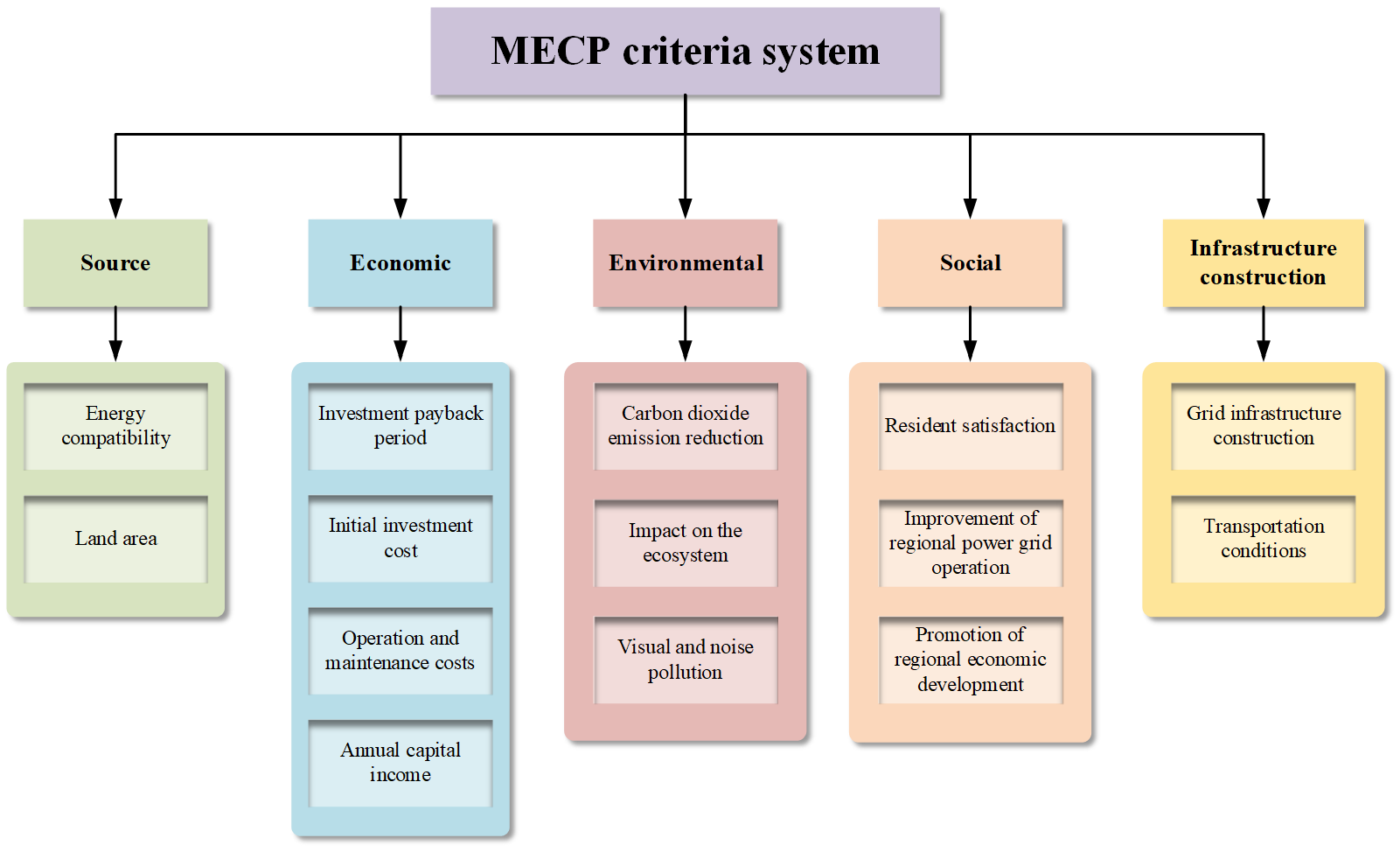
In real-world decision-making environments, the investment evaluation of MECS is influenced by multiple criteria reflecting different aspects. It is crucial to establish a universal standard system. In summary, resources, economy, environment, society, and infrastructure are the main criteria for investment evaluation. These must be comprehensively considered to make optimal decisions. The criteria are established based on the defined objectives, research areas, data accessibility, and operational methods. To develop a more comprehensive and logical framework, experts have been consulted, in-depth literature reviews were conducted, and discussions took place to identify and define the decision factors in each area. The 14 criteria used in this research were finally selected by the decision-making committee, considering the uniqueness of the MECS, as illustrated in Figure 1: The Investment evaluation criteria system for MECS. They include the following five aspects.
3.1. Resources Criteria
Energy compatibility (C1): This indicator assesses how well the energy characteristics and quantity at the project’s site align with the energy demands of a specific multi-energy complementary system. It indicates whether the energy available can adequately support the system’s normal operation, fulfill its intended functions, and achieve efficient utilization.
Land area (C2): This reflects the resource-bearing capacity of the region. A larger land area means more space to arrange energy facilities such as solar panels and wind turbines [15].
3.2. Economic Criteria
Investment payback period (C3): This denotes the period needed for the total revenue from the initiative to equal the initial investment. The capital turnover rate and the project’s economic benefits are effectively represented by the investment payback period [14].
Initial investment cost (C4): This refers to the total funds invested at the beginning of the project to ensure its proper operation. It mainly includes equipment purchase costs, engineering construction costs, supporting facilities construction costs, and preliminary planning and design costs [4,14,16].
Operation and maintenance costs (C5): This refers to the total costs necessary for the proper functioning of the multi-energy complementary project once it is operational. It mainly includes equipment maintenance costs, employee salaries, and consumables costs [4,14,16].
Annual capital income (C6): This refers to the economic benefits related to capital investment that the project obtains within a year. It mainly includes electricity sales income, heating (cooling) income, other energy product sales income, and government subsidies and preferential policy income.
3.3. Environmental Criteria
Carbon dioxide emission reduction (C7): The specific meaning of carbon dioxide emission reduction is the reduction in CO2 emissions compared to traditional single thermal power generation when the multi-energy complementary system generates power using renewable energy sources. This indicator is significant in terms of carbon neutrality goals and emphasizes the importance of developing multi-energy complementary systems. However, the CO2 reduction varies across different multi-energy complementary systems, making it an important evaluation criterion [4,14,16,68].
Impact on the ecosystem (C8): Multi-energy complementary projects require land, which inevitably affects local soil, vegetation, water resources, and other wildlife. Therefore, it is necessary to assess the ecological harmony of different projects to meet the requirements of sustainable development [4,14,18].
Visual and noise pollution (C9): This refers to the potential noise generated by wind turbines in the wind farm, which may disturb nearby residents, as well as the visual impact of large areas of solar panels and wind turbines altering the natural landscape and negatively affecting the surrounding environment.
3.4. Social Criteria
Resident satisfaction (C10): Resident satisfaction refers to the local residents’ perception of the reliability of the electricity provided by the multi-energy complementary system and their direct experience of environmental improvements. It reflects both the system’s reliability and its emission reduction benefits as felt by residents [4,14,68].
Improvement of regional power grid operation (C11): This refers to the beneficial effect of the MECS on the functioning of the regional power grid. It includes factors such as the grid’s reliability post-integration, power quality, energy efficiency, and the ability to adjust grid load.
Promotion of regional economic development (C12): Multi-energy complementary projects cover various industries, such as energy production, transmission, storage, equipment manufacturing, installation, and maintenance. These projects can stimulate the growth of local industries, create numerous job opportunities, and contribute to economic value-added [68].
3.5. Infrastructure Construction
Grid infrastructure construction (C13): Refers to investments in completed grid construction, transmission line construction, and substation equipment construction [15].
Transportation conditions (C14): This refers to the ease of transporting heavy machinery and staff, which is a crucial consideration for the development and upkeep of the project [16].
4. Research Methodology
4.1. Preliminaries
Pythagorean fuzzy sets (PFS) were proposed by Yager in 2014 as an enhancement of intuitionistic fuzzy sets, aimed at handling fuzziness and uncertainty in descriptive information [69]. That same year, Zhang extended the mathematical equations and core algorithms of PFS, laying the groundwork for its practical applications [70]. The following is a brief introduction to the relevant definitions and algorithms:
Definition 1. Let X be a universe of discourse. A PFS A in X is defined as:
where $${\mu }_{p}\left(x\right)$$ and $${v}_{p}\left(x\right)$$ denote the membership degree and non-membership degree of element x to A, respectively. Here, $${\mu }_{p}\left(x\right):X\to \left[0,1\right]$$ and $${v}_{p}\left(x\right):X\to \left[0,1\right]$$ are functions such that for every $$x\in X$$:$$0\le {\mu }_{p}{\left(x\right)}^{2}+{v}_{p}{\left(x\right)}^{2}\le 1$$. Additionally, the hesitancy degree $${\pi }_{p}\left(x\right)$$ of any element $$x\in X$$ is defined as:
Definition 2. [71]. Let the complement of $$p$$ be denoted as $${p}^{c}$$, then $${p}^{c}$$ is defined as:
Definition 3. [71,72]. Let there be three PFSs, defined as$$\,\alpha =\left({\mu }_{\alpha },{v}_{\alpha }\right)$$, $${\alpha }_{1}=\left({\mu }_{1},{v}_{1}\right)$$, $${\alpha }_{2}=\left({\mu }_{2},{v}_{2}\right)$$, the algebraic operations between them are presented as follows:
Definition 4. [72]. Let $$\alpha =\left({\mu }_{\alpha },{v}_{\alpha }\right)$$, then the score function of $$\alpha$$ is defined as:
It is evident that the larger $$S\left(\alpha \right)\in \left[0,1\right]$$, the larger the PFS.
Definition 5. [73]. Let $$\alpha_1 = \left( \mu_1, v_1 \right)\,{\alpha }_{2}=\left({\mu }_{2},{v}_{2}\right)$$ be two PFS the distance between $${\alpha }_{1}$$ and $${\alpha }_{2}$$ is follows:
Definition 6. [73]. Let there be n PFNs $$\stackrel{\sim }{{p}_{1}},\stackrel{\sim }{{p}_{2}},...,\stackrel{\sim }{{p}_{n}}$$, then their Pythagorean Fuzzy Aggregation (PFAG) operator is as follows:
4.2. Evaluation Methods and Decision Framework
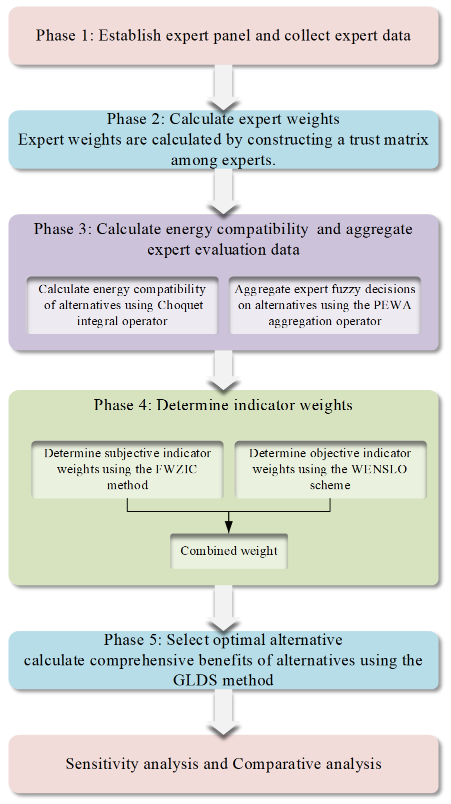
As illustrated in Figure 2, a five-stage decision-making framework is presented to select the MECS that provides the highest overall benefits. A detailed explanation of the various stages of the research approach is given in this section.
4.2.1. Phase 1—Collecting Expert Data
Step 1. Assemble a panel of five experts in the field to create an expert committee. The experts are requested to evaluate each criterion according to Table 1 and assess the alternative solutions under each criterion based on Table 2.
Experts evaluated the importance of the 14 evaluation indicators {C1, …, C14} linguistically according to linguistic variables, resulting in the indicator importance matrix. For example, Expert E1 rated Indicator C1 as “VVI”, corresponding to the PFS [0.90, 0.20].
According to linguistic variables, experts linguistically evaluated the performance of the five alternatives {A1, …, A5} against each indicator, yielding five independent evaluation matrices. For example, Expert E1 rated Alternative A5 under Indicator C2 as “VH”, corresponding to the PFS [0.80, 0.25].
To ensure the reliability and validity of the expert judgments, the expert panel was deliberately composed of five specialists from academia, industry, and government, each with over five years of experience in multi-energy systems. Evaluations were conducted independently using standardized linguistic scales to avoid mutual influence and anchoring bias. The use of Pythagorean fuzzy sets further captures the inherent uncertainty and hesitancy in subjective judgments, mitigating potential bias. Consistency among experts was examined using Kendall’s W coefficient based on the importance rankings of criteria. The calculated W = 0.73 (p < 0.01) indicates a high level of agreement, confirming the reliability of the elicited judgments. Moreover, objective input data were sourced from official statistics and cross-checked by independent researchers, ensuring data accuracy.
Table 1. Linguistic variables for evaluating the relative importance of criteria.
|
Linguistic Variables |
PFNS |
|---|---|
|
Very very important (VVI) |
[0.90, 0.20] |
|
Very important (VI) |
[0.80, 0.25] |
|
Important (I) |
[0.70, 0.35] |
|
Medium important (MI) |
[0.60, 0.50] |
|
Medium (M) |
[0.50, 0.60] |
|
Medium unimportant (MU) |
[0.45, 0.70] |
|
Unimportant (U) |
[0.40, 0.75] |
|
Very unimportant (VU) |
[0.20, 0.80] |
|
Very very unimportant (VVU) |
[0.10, 0.90] |
Table 2. Linguistic variables for relative importance ratings of alternative solutions.
|
Linguistic Variables |
PFNS |
|---|---|
|
Extremely high (EH) |
[1.00, 0.00] |
|
Very very high (VVH) |
[0.90, 0.20] |
|
Very high (VH) |
[0.80, 0.25] |
|
High (H) |
[0.70, 0.35] |
|
Medium high (MH) |
[0.60, 0.50] |
|
Medium (M) |
[0.50, 0.60] |
|
Medium low (ML) |
[0.45, 0.70] |
|
Low (L) |
[0.40, 0.75] |
|
Very low (VL) |
[0.20, 0.80] |
|
Very very low (VVL) |
[0.10, 0.90] |
4.2.2. Phase 2—Calculating Expert Weights
In order to determine expert weights in a scientific and rational manner, a trust matrix is established by considering the differing levels of confidence in the assessments provided by the experts. This matrix reflects both the self-trust of each expert and the trust levels between experts, which are then used to calculate the expert weights. The specific steps are as follows:
Step 2. A 5-point Likert scale was used to collect the mutual trust degree among experts, and the trust matrix Γ was constructed as follows:
where $${\gamma }_{kk}$$ is the degree of trust that $${E}_{k}$$ has in himself, and $${\gamma }_{ij}$$ is the degree of trust that $${E}_{i}$$ has in $${E}_{j}$$.
Step 3. Determine the total trust degree $${\Theta }_{i}$$ of expert $${E}_{i}$$ based on the trust matrix.
Step 4. Determine the expert weights $${\lambda }_{i}$$ based on $${\Theta }_{i}$$, with the equation as follows:
4.2.3. Phase 3—Calculating Energy Compatibility and Aggregating Expert Evaluation Data
Calculating Energy Compatibility
The energy compatibility indicator is a key metric reflecting the universality of this evaluation framework. Its calculation requires selecting different indicators according to distinct MECSs. For example, an MECS project integrating wind, solar, and hydropower energy (with energy storage) involves wind, solar, and hydropower resources. Thus, three indicators can be selected to represent the regional energy richness: annual effective wind speed hours, annual average sunshine hours, and theoretical hydropower resource reserves. After selecting the indicators, the calculation is performed using the Choquet integral operator. The comprehensive calculation process is outlined below:
Step 5. Normalize the data by leveraging both the actual data $${t}_{ij}$$ from the project’s host region and the ideal data $${i}_{ij}$$ required by the project.
where i represents an alternative solution, m represents the quantity of possible alternative solutions, j signifies the energy type used in the project, n represents the number of energy types, $${t}_{ij}$$ indicates the actual energy data of the region, and $${i}_{ij}$$ denotes the ideal energy data required by the project.
Example: in Scheme 2, $${S}_{21}=5475/6000=0.91;{S}_{22}=2000/3200=0.63;{S}_{23}=67/93=0.72.$$
Step 6. Sort the normalized data in descending order, with the equation as follows:
Example: Sort Sij in descending order:$$f\left({S}_{\left(21\right)}\right)\ge f\left({S}_{\left(23\right)}\right)\ge f\left({S}_{\left(22\right)}\right)$$.
Step 7. The fuzzy measures for each subset are defined based on the proportion of each energy source relative to the total energy sources used in the project, using the following equation:
Example: The fuzzy density of each energy source is determined according to the proportion of the project installed capacity:
|
```latex\mu \left(\left\{{S}_{21}\right\}\right)=\frac{{S}_{21}}{\sum\limits_{j=1}^{n}{S}_{2j}}=\frac{300}{300+500+200}=0.3;``````latex\mu \left(\left\{{S}_{21},{S}_{22}\right\}\right)=\frac{{S}_{21}+{S}_{22}}{\sum\limits_{j=1}^{n}{S}_{ij}}=\frac{300+500}{300+500+200}=0.8;``````latex\mu \left(\left\{{S}_{21},{S}_{22},{S}_{23}\right\}\right)=1``` |
Step 8. Calculate the cumulative weights: for each i, compute the difference $$\Delta {\mu }_{ij}$$ in fuzzy measures between the first i elements.
Example: $$\Delta {\mu }_{21}=0.3;\Delta {\mu }_{22}=0.8-0.3=0.5;\Delta {\mu }_{23}=1-0.8=0.2.$$
Step 9. Weighted summation $$C\mu \left({f}_{i}\right)$$: multiply the sorted values by the corresponding $$\Delta {\mu }_{ij}$$ and sum them up, with the equation as follows:
Example: $$C\mu \left({f}_{2}\right)=0.3*0.91+0.5*0.63+0.2*0.72=0.73$$.
Aggregating Expert Evaluation Data
In this stage, the PFWA is adopted to aggregate the evaluations of alternative solutions under each criterion by various experts into a comprehensive evaluation matrix.
Step 10. Combine the decision matrices and obtain a comprehensive decision matrix $${R}_{ij}={\left[{R}_{ij}\right]}_{n×m}$$ by using $$PFWA$$:
where $${R}_{ij}^{k}$$ represents the evaluation given by the Ek for $${C}_{j}$$ in alternative solution $${A}_{i}$$, $${\lambda }_{k}$$ denotes the weight of the Ek, and q is the number of experts.
4.2.4. Phase 4—Determining Indicator Weights
During this phase, the FWZIC method is applied to assess the subjective weights of the indicators, while the WENSLO method is employed to calculate the objective weights. Ultimately, the comprehensive weights are combined using a linear weighting approach.
Determine Subjective Indicator Weights Based on the FWZIC Method
Step 11. First, The matrix (E, C) composed of experts’ linguistic evaluations on the importance of indicators is shown as an Equation (20). Then, calculate the ratio of the fuzzified data $$\tilde{E}_t : \tilde{C}_{ij}$$ according to Equation (7), Equation (10) and Equation (21). The equation is shown as follows:
wherein $$\mathrm{Im}p\left({E}_{ij}/{C}_{y}\right)$$ is the importance level based on each criterion of each expert, and $$\mathrm{Im}p\left(\stackrel{\sim }{{E}_{ij}}/\stackrel{\sim }{{C}_{y}}\right)$$ denotes the fuzzy number of such importance.
Step 12. First, defuzzify $${\stackrel{\sim }{E}}_{t}:\stackrel{\sim }{{C}_{ij}}$$ using Equation (8), and then calculate the fuzzy number of the final weight $$\stackrel{\sim }{{w}_{j}}$$ as follows:
Step 13. Normalize the $$\stackrel{\sim }{{w}_{j}}$$ to obtain the final subjective weights $${{w}_{j}}^{s}$$ as follows:
Determine Objective Indicator Weights Based on the WENSLO Method
Step 14. First, defuzzify the experts’ evaluation matrix $$R_{ij} = \left[ R_{ij} \right]_{n \times m}$$ through Equation (8), and then obtain the decision matrix $$\xi(A, C)$$ based on the defuzzified data, which is in the following form:
where, A denotes the alternative solutions, m represents the number of alternatives, C stands for the criteria, and j indicates the number of criteria. For benefit-type indicators, fill in the maximum value of expert evaluations, while for cost-type indicators, fill in the minimum value.
Step 15. Data Standardization: Matrix $$\xi \left(A,C\right)$$ is normalized to obtain a dimensionless decision matrix $${z}_{ij}$$. The following equation was used as the method for linear normalization:
The result is a standardized decision matrix$${\left[{z}_{ij}\right]}_{m×n}$$:
Step 16. Calculation of Criterion Class Intervals. The size of the j-th criterion class interval $$\Delta {z}_{j}$$ is calculated by Sturges’ rule as:
Step 17. According to Equation (28) calculate the index slope $$\mathit{tan}{\varphi }_{j}$$ based on the matrix $${\left[{z}_{ij}\right]}_{m×n}$$.
Step 18. Index envelope determination: According to Equation (29), calculate the index envelope $${E}_{j}$$ based on matrix $${\left[{z}_{ij}\right]}_{m×n}$$. This total Euclidean distance represents the envelope of the index.
Step 19. The slope ratio $${q}_{j}$$ calculated as the ratio of the $${E}_{j}$$ to the $$\mathit{tan}{\varphi }_{j}$$:
Step 20. Calculation of criterion weights: Calculate the objective indicator weights $${{w}_{j}}^{o}$$ based on $${q}_{j}$$:
Determination of Comprehensive Index Weights
Step 21. Calculate the overall weights $${w}_{j}$$ of the criterions based on $${{w}_{j}}^{s}$$and $${{w}_{j}}^{o}$$ using the equation below:
4.2.5. Phase 5—Selecting the Optimal Alternative
At this phase, the paper integrates prospect theory with the GLDS method and expands it into the PHFS environment. The specific process is shown in Figure 3. The detailed calculation process is as follows:
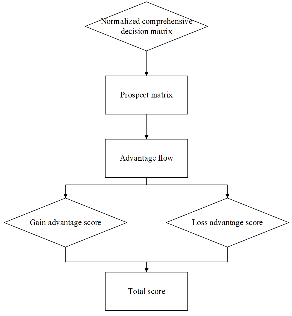
Step 22. Standardize the comprehensive decision matrix. Normalize $$R_{ij}=\left[R_{ij}\right]_{n\times m}$$ to $$R_{ij}^N$$ according to the attribute of the indices, as shown in Equation (33). Then, defuzzify the normalized matrix using Equation (9):
where $${C}^{B}$$ represents benefit indices and $${C}^{S}$$ represents cost indices.
Step 23. Select the reference point $$\hat{t}$$ according to the decision-maker’s risk preference and mental condition. Typical reference points include the zero point, median, mean, optimal value, and worst value. In this study, the median is selected as the reference point.
Example: The values of Indicator C1 are derived from the energy compatibility scores (0.67, 0.73, 0.63, 1.00, 0.83). The median value after sorting is 0.73, which is consistent with the reference point of C1. All reference points are shown.
Step 24. Obtain the prospect matrix $$\psi=\left(\psi_{ij}\right)_{m\times n}$$ according to the Equation (34), where $$\Delta t_{ij}$$ denotes the distance between the evaluation value and the reference point. A positive $$\Delta {t}_{ij}>0$$ represents a gain, while a negative value indicates a loss:
where τ and k denote the exponential parameters for gains and losses, respectively, satisfying $$\tau ,k\in \left[0,1\right]$$. η represents the risk aversion parameter, satisfying $$\eta >1$$. Studies have shown that prospect theory is most effective when $$k=\tau =0.88$$, and $$\eta =2.25$$, so this paper also selects these three parameters.
Example: For A1C1, $${R}_{11}^{\mathrm{N}}=0.67,\hat{t}=0.73,\Delta {t}_{11}=-0.06$$, then $${\Psi }_{11}=-2.25*{\left(0.06\right)}^{0.88}=-0.19$$. All prospect values form the prospect matrix.
Step 25. Based on the $$\psi ={\left({\psi }_{ij}\right)}_{m×n}$$, calculate the advantage flow $${\Xi }_{j}\left({A}_{i},{A}_{b}\right)$$ of the alternative solution $${A}_{i}\left(i=1,2,...,m\right)$$ relative to the alternative solution $${A}_{b}\left(b=1,2,...,m\right)$$ under index $${C}_{j}\left(j=1,2,...,n\right)$$, and its normalized value $${\Xi }_{j}^{N}\left({A}_{i},{A}_{b}\right)$$, with the equations as follows:
Example: Taking Indicator C1 as an example, a comparison is made between A5 and A1:
Step 26. Calculate the gain advantage score $${\stackrel{\sim }{\Xi }}_{j}\left({A}_{i}\right)$$ of each alternative for each indicator, then sum them up by weight to get the comprehensive dominance score $$\overset{\sim}{\operatorname*{\operatorname*{\Xi^*}}}\left(A_i\right)$$, and its normalized value $$\tilde{\Xi}^{*N}\left(A_i\right)$$. With the equations as follows:
Step 27. Arrange the $$\tilde{\Xi}^{*N}\left(A_i\right)$$ of each alternative in descending order to establish the priority ranking of each alternative, represented as $$\sum\nolimits_1=\left\{\sigma_1\left(A_1\right),\sigma_1\left(A_2\right),...,\sigma_1\left(A_m\right)\right\}$$.
Step 28. Determine the loss advantage score $${\underset{\sim }{\Xi }}_{j}\left({A}_{i}\right)$$ of alternative Ai under criterion Cj, then sum them up by weight to get the comprehensive loss advantage score $$\underset{\sim }{\Xi }^*\left({A}_{i}\right)$$ and its normalized value $$\underset{\sim }{\Xi }^{{*}{N}}\left({A}_{i}\right)$$. With the equations as follows:
Step 29. Sort the $$\underset{\sim }{\Xi }^{{*}{N}}\left({A}_{i}\right)$$ of each alternative in ascending order to obtain the priority ranking of each alternative, denoted as $$\sum\nolimits_2=\begin{Bmatrix}\sigma_2\begin{pmatrix}A_1\end{pmatrix},\sigma_2\begin{pmatrix}A_2\end{pmatrix},...,\sigma_2\begin{pmatrix}A_m\end{pmatrix}\end{Bmatrix}$$.
Step 30. The total score $$S_i^*$$ of an alternative is determined by $$\tilde{\Xi}^{*N}\left(A_i\right)$$ and $$\underset{\sim }{\Xi }^{{*}{N}}\left({A}_{i}\right)$$, as shown in Equation (43). The final optimal alternative is the one with the highest total score.
where m represents the overall count of options, and $${\sigma }_{e}\left({A}_{i}\right),e=1,2$$ is the priority order of alternative Ai.
5. Empirical Analysis
In order to thoroughly assess the practical value of the evaluation framework in project investment decision-making, this study carefully reviewed a wide range of MECS projects approved by the Hebei Provincial Development and Reform Commission. Ultimately, five representative projects were selected as the focus of the empirical research. These projects cover different fields and scales, showing diversified characteristics in the investment environment, construction period, expected returns, etc. The constructed evaluation framework was used to conduct a detailed analysis of the projects, leading to the selection of the optimal investment target. The detailed information of these projects is presented in Table 3. All five MECS alternatives selected for empirical analysis are equipped with large-scale lithium-ion energy storage systems, which are the core components to ensure the stability of energy supply and the synergistic operation of multiple energy sources. For lithium-ion battery energy storage systems, effective thermal management is essential to ensure their operational safety, performance stability, and service life, and numerous advanced thermal management strategies and practical operational constraints have been proposed and verified in recent research [74]. The energy storage systems of the selected projects all adopt mature thermal management schemes, which lay a solid foundation for the reliable operation of the MECS.
Table 3. Information of alternatives.
|
Alternative |
Project Name |
Location |
Multi-Energy Complementary Pattern and Scale |
|---|---|---|---|
|
A1 |
Dacheng Multi-energy Complementary New Energy Comprehensive Demonstration Project |
Dacheng County, Langfang City |
Wind Power 100 MW + PV 250 MW + Energy Storage 70 MW/140 MWh + Hydrogen Production 1000 Nm3/h |
|
A2 |
Agro-Pastoral Photovoltaic-Wind-Hydro-Storage Multi-energy Complementary Smart Energy Demonstration Project of SPIC Fengning Green Energy Co., Ltd. |
Chengde City, Fengning County |
Wind Power 300 MW + PV 500 MW + Pumped Storage 200 MW + Energy Storage 160 MW/320 MWh + Hydrogen Production 20,000 Nm3/h + Charging & Battery Swapping Station 15 MW |
|
A3 |
Fengning Qirun 1000 MW Multi-energy Complementary Integration Optimization Demonstration Project |
Chengde City, Fengning County |
PV 1000 MW + Energy Storage 200 MW/400 MWh + Hydrogen Production 10,000 Nm3/h + 100,000 m2 Heating |
|
A4 |
Yuxian Multi—energy Complementary Demonstration Project |
Zhangjiakou City, Yuxian County |
Wind Power 250 MW + PV 750 MW + Energy Storage 200 MW/200 MWh + Big Data Center Load 344 MW |
|
A5 |
Chengde Hangkong Tianqi Wind + PV + Storage + Hydrogen Integrated Multi-energy Complementary Demonstration Project |
Weichang Manchu and Mongol Autonomous County, Chengde City |
Wind Power 300 MW + PV 200 MW + Energy Storage 100 MW/200 MWh + Hydrogen Production 3000 Nm3/h |
5.1. Phase 1—Collecting Expert Data
In this phase, first, we invited five decision-makers and experts in the MECS (Multi-energy Complementary Project) field to form an expert panel. We screened basic information on feasible alternatives by reviewing industry reports and government documents. Through literature reviews and expert consultations, we identified the indicators affecting MECS investment evaluation and established an evaluation index system consisting of 14 indicators. For detailed descriptions, please refer to the “Construction of the Evaluation Criteria System” section. Subsequently, experts were requested to assess each indicator and option. The results of the evaluation are presented in Table 4 and Table 5.
Table 4. Experts’ evaluation of each indicator.
|
C1 |
C2 |
C3 |
C4 |
C5 |
C6 |
C7 |
C8 |
C9 |
C10 |
C11 |
C12 |
C13 |
C14 |
|
|---|---|---|---|---|---|---|---|---|---|---|---|---|---|---|
|
E1 |
VVI |
M |
I |
VI |
I |
VI |
MI |
MI |
MI |
M |
MI |
M |
MU |
M |
|
E2 |
VI |
MI |
VI |
I |
VI |
I |
MI |
M |
M |
MI |
M |
MI |
M |
M |
|
E3 |
VI |
M |
I |
VI |
MI |
I |
MI |
MI |
MI |
M |
MU |
MU |
M |
M |
|
E4 |
VVI |
M |
I |
I |
MI |
VI |
MI |
M |
MI |
MI |
MI |
MI |
M |
M |
|
E5 |
VVI |
M |
VI |
I |
MI |
I |
M |
M |
I |
M |
MI |
MU |
MI |
MI |
Note: Very very important (VVI); Very important (VI); Important (I); Medium important (MI); Medium (M); Medium unimportant (MU).
Table 5. Experts’ evaluation of each alternative.
|
C2 |
C3 |
C4 |
C5 |
C6 |
C7 |
C8 |
C9 |
C10 |
C11 |
C12 |
C13 |
C14 |
||
|---|---|---|---|---|---|---|---|---|---|---|---|---|---|---|
|
A1 |
E1 |
H |
VH |
M |
M |
H |
H |
ML |
H |
MH |
VH |
M |
ML |
VVH |
|
E2 |
L |
M |
M |
L |
H |
H |
VH |
VL |
MH |
MH |
VH |
VH |
VVH |
|
|
E3 |
M |
H |
MH |
ML |
H |
M |
L |
L |
H |
H |
M |
VH |
VH |
|
|
E4 |
VL |
M |
M |
ML |
MH |
M |
L |
M |
MH |
M |
M |
VH |
VH |
|
|
E5 |
ML |
H |
M |
MH |
H |
M |
ML |
L |
H |
ML |
M |
VH |
VH |
|
|
A2 |
E1 |
VH |
MH |
VH |
VH |
VVH |
VVH |
H |
VH |
VH |
VVH |
H |
H |
ML |
|
E2 |
VH |
VH |
H |
VVH |
VVH |
VH |
H |
M |
H |
H |
VVH |
MH |
L |
|
|
E3 |
H |
VH |
H |
H |
H |
MH |
H |
M |
VH |
VH |
MH |
M |
ML |
|
|
E4 |
VH |
H |
VH |
M |
VH |
H |
MH |
MH |
VH |
VH |
H |
ML |
L |
|
|
E5 |
H |
VH |
VH |
VH |
VH |
H |
M |
L |
VH |
VH |
MH |
M |
MH |
|
|
A3 |
E1 |
VVH |
ML |
VVH |
VH |
VH |
VH |
MH |
H |
VVH |
H |
H |
H |
ML |
|
E2 |
VH |
H |
VH |
VH |
VVH |
H |
M |
ML |
H |
VH |
H |
MH |
L |
|
|
E3 |
H |
H |
VH |
M |
VH |
H |
H |
L |
VH |
H |
MH |
M |
ML |
|
|
E4 |
VH |
VH |
H |
MH |
H |
VH |
H |
H |
VVH |
MH |
VH |
ML |
L |
|
|
E5 |
H |
VH |
H |
VH |
VH |
H |
MH |
H |
VH |
VH |
H |
M |
MH |
|
|
A4 |
E1 |
H |
M |
M |
L |
MH |
ML |
MH |
M |
M |
H |
M |
M |
M |
|
E2 |
H |
H |
H |
M |
H |
M |
VVH |
L |
VH |
H |
M |
M |
H |
|
|
E3 |
M |
MH |
M |
H |
M |
MH |
L |
VL |
H |
H |
M |
MH |
MH |
|
|
E4 |
L |
M |
M |
M |
H |
ML |
L |
M |
H |
VH |
H |
MH |
H |
|
|
E5 |
M |
MH |
M |
H |
M |
ML |
M |
H |
M |
M |
H |
MH |
H |
|
|
A5 |
E1 |
VH |
MH |
ML |
MH |
VH |
H |
M |
ML |
M |
H |
ML |
L |
H |
|
E2 |
M |
ML |
M |
ML |
H |
VVH |
M |
L |
H |
MH |
H |
H |
M |
|
|
E3 |
VH |
H |
M |
L |
VH |
H |
M |
VL |
H |
H |
M |
M |
M |
|
|
E4 |
VH |
ML |
ML |
L |
M |
H |
M |
H |
VH |
H |
M |
M |
M |
|
|
E5 |
VH |
M |
MH |
H |
H |
MH |
ML |
MH |
MH |
H |
MH |
M |
M |
|
Note: Very very high (VVH); Very high (VH); High (H); Medium high (MH); Medium (M); Medium low (ML); Low (L); Very low (VL).
5.2. Phase 2—Determining Expert Weights
In the second phase, experts evaluated the trustworthiness of each expert using the criteria in Table 6. Calculations were then performed according to the Equation (12) and Equation (13). The final expert weights are as follows: λ1 = 0.22, λ2 = 0.15, λ3 = 0.24, λ4 = 0.17, λ5 = 0.22.
Table 6. Five-point likert scale.
|
Scale |
Explanation |
|---|---|
|
1 |
Very distrust |
|
2 |
Distrust |
|
3 |
Medium |
|
4 |
Trust |
|
5 |
Very trust |
5.3. Calculating Energy Compatibility and Aggregating Expert Decision Data
5.3.1. Calculating Energy Compatibility
The five alternatives involve three energy resources: wind energy, solar energy, and hydropower resources. Based on these three energy types, we selected three indicators—annual effective wind speed hours, annual average sunshine hours, and theoretical reserve of hydropower resources—to calculate the energy compatibility of each alternative. Data for each alternative collected through the investigation are presented in Table 7.
Table 7. Resource data of each alternative.
|
Alternative |
Criterions |
tij |
iij |
Sij |
|---|---|---|---|---|
|
A1 |
Annual Effective Wind Speed Hours (h) |
3813 |
6000 |
0.64 |
|
Annual Average Sunshine Hours (h) |
2200 |
3200 |
0.69 |
|
|
A2 |
Annual Effective Wind Speed Hours (h) |
5475 |
6000 |
0.91 |
|
Annual Average Sunshine Hours (h) |
2000 |
3200 |
0.63 |
|
|
Theoretical Reserve of Hydropower Resources (MW) |
67 |
93 |
0.72 |
|
|
A3 |
Annual Average Sunshine Hours (h) |
2000 |
3200 |
0.625 |
|
A4 |
Annual Effective Wind Speed Hours (h) |
7000 |
6000 |
1.17 |
|
Annual Average Sunshine Hours (h) |
3000 |
3200 |
0.94 |
|
|
A5 |
Annual Effective Wind Speed Hours (h) |
5475 |
6000 |
0.91 |
|
Annual Average Sunshine Hours (h) |
2300 |
3200 |
0.72 |
According to Equation (15), Equation (16), Equation (17) and Equation (18), resource data of each alternative were calculated. The final energy compatibility of each alternative is shown in Table 8.
Table 8. Energy compatibility of each alternative.
|
$$\bm{C}\bm{\mu }\left({\bm{f}}_{\bm{i}}\right)$$ |
Score |
|---|---|
|
$$C\mu \left({f}_{1}\right)$$ |
0.67 |
|
$$C\mu \left({f}_{2}\right)$$ |
0.73 |
|
$$C\mu \left({f}_{3}\right)$$ |
0.63 |
|
$$C\mu \left({f}_{4}\right)$$ |
1 |
|
$$C\mu \left({f}_{5}\right)$$ |
0.83 |
5.3.2. Aggregating Expert Data
Using Equation (19), experts’ evaluation of each alternative. was integrated into a detailed assessment matrix, and the outcomes are provided in Table 9.
Table 9. Experts’ comprehensive evaluation matrix.
|
Criterion |
A1 |
A2 |
A3 |
A4 |
A5 |
|---|---|---|---|---|---|
|
C2 |
[0.44, 0.67] |
[0.76, 0.29] |
[0.80, 0.28] |
[0.58, 0.51] |
[0.77, 0.29] |
|
C3 |
[0.68, 0.39] |
[0.75, 0.31] |
[0.73, 0.34] |
[0.58, 0.51] |
[0.57, 0.53] |
|
C4 |
[0.53, 0.57] |
[0.77, 0.29] |
[0.80, 0.27] |
[0.54, 0.55] |
[0.51, 0.61] |
|
C5 |
[0.49, 0.63] |
[0.77, 0.30] |
[0.73, 0.35] |
[0.60, 0.49] |
[0.54, 0.57] |
|
C6 |
[0.69, 0.37] |
[0.83, 0.25] |
[0.81, 0.26] |
[0.60, 0.49] |
[0.73, 0.33] |
|
C7 |
[0.59, 0.49] |
[0.77, 0.32] |
[0.74, 0.31] |
[0.50, 0.63] |
[0.73, 0.35] |
|
C8 |
[0.53, 0.59] |
[0.65, 0.42] |
[0.63, 0.44] |
[0.62, 0.54] |
[0.49, 0.62] |
|
C9 |
[0.51, 0.61] |
[0.60, 0.50] |
[0.62, 0.47] |
[0.51, 0.59] |
[0.51, 0.60] |
|
C10 |
[0.66, 0.42] |
[0.79, 0.26] |
[0.84, 0.24] |
[0.65, 0.42] |
[0.67, 0.40] |
|
C11 |
[0.65, 0.44] |
[0.82, 0.25] |
[0.71, 0.35] |
[0.69, 0.37] |
[0.69, 0.37] |
|
C12 |
[0.57, 0.53] |
[0.72, 0.38] |
[0.75, 0.33] |
[0.60, 0.49] |
[0.55, 0.55] |
|
C13 |
[0.76, 0.31] |
[0.57, 0.53] |
[0.57, 0.53] |
[0.57, 0.53] |
[0.52, 0.58] |
|
C14 |
[0.85, 0.23] |
[0.48, 0.66] |
[0.48, 0.66] |
[0.64, 0.43] |
[0.56, 0.53] |
5.4. Phase 4—Determining Indicator Weights
In this phase, first, the subjective weights of indicators were calculated using Equation (21), Equation (22) and Equation (23), then the objective weights of indicators were computed via Equation (24), Equation (25), Equation (26), Equation (27), Equation (28), Equation (29), Equation (30) and Equation (31), and finally, the comprehensive indicator weights were determined by Equation (32), as shown in Table 10.
Table 10. Criterion weight.
|
Criterion |
Subjective Weight |
Objective Weight |
Comprehensive Weight |
|---|---|---|---|
|
C1 |
0.106 |
0.108 |
0.107 |
|
C2 |
0.058 |
0.016 |
0.037 |
|
C3 |
0.091 |
0.0103 |
0.097 |
|
C4 |
0.091 |
0.154 |
0.123 |
|
C5 |
0.076 |
0.080 |
0.078 |
|
C6 |
0.091 |
0.085 |
0.088 |
|
C7 |
0.066 |
0.087 |
0.077 |
|
C8 |
0.060 |
0.086 |
0.073 |
|
C9 |
0.071 |
0.080 |
0.076 |
|
C10 |
0.060 |
0.034 |
0.047 |
|
C11 |
0.062 |
0.034 |
0.048 |
|
C12 |
0.056 |
0.022 |
0.039 |
|
C13 |
0.056 |
0.034 |
0.045 |
|
C14 |
0.058 |
0.078 |
0.068 |
5.5. Stage 5—Select the Optimal Alternative
In this stage, the expert comprehensive decision matrix is first normalized using Equation (33), and then the normalized matrix is defuzzified following Equation (8). Then, a reference point is selected based on the decision-makers’ risk preferences and psychological states. In this study, the median is chosen as the reference point, specifically as shown in Table 11. Subsequently, the prospect matrix is obtained according to Equation (34), as presented in Table 12.
Next, the comprehensive gain dominance scores of alternative Ai are calculated and ranked using Equation (35), Equation (36), Equation (37), Equation (38) and Equation (39), as shown in Table 13. The comprehensive loss dominance scores of alternatives Ai are calculated and ranked according to Equation (40), Equation (41) and Equation (42), as listed in Table 14. Finally, the comprehensive scores of each alternative are computed using Equation (43). The ranking result is A5 > A4 > A1 > A2 > A3, as shown in Table 15.
Table 11. Reference point.
|
C1 |
C2 |
C3 |
C4 |
C5 |
C6 |
C7 |
|
|---|---|---|---|---|---|---|---|
|
$$\hat{t}$$ |
0.73 |
0.54 |
0.39 |
0.52 |
0.48 |
0.71 |
0.71 |
|
C8 |
C9 |
C10 |
C11 |
C12 |
C13 |
C14 |
|
|
$$\hat{t}$$ |
0.56 |
0.62 |
0.64 |
0.67 |
0.56 |
0.52 |
0.52 |
Table 12. Prospect matrix.
|
C1 |
C2 |
C3 |
C4 |
C5 |
C6 |
C7 |
C8 |
C9 |
C10 |
C11 |
C12 |
C13 |
C14 |
|
|---|---|---|---|---|---|---|---|---|---|---|---|---|---|---|
|
A1 |
−0.19 |
−0.47 |
0 |
0.02 |
0.15 |
−0.13 |
−0.45 |
0.08 |
0 |
−0.04 |
−0.19 |
−0.13 |
0.26 |
0.36 |
|
A2 |
0 |
0.25 |
−0.29 |
−0.71 |
−0.50 |
0.13 |
0.06 |
−0.45 |
−0.27 |
0.18 |
0.17 |
0.17 |
0 |
−0.35 |
|
A3 |
−0.3 |
0.28 |
−0.07 |
−0.73 |
−0.35 |
0.11 |
0.03 |
−0.40 |
−0.37 |
0.22 |
0.03 |
0.21 |
0 |
−0.35 |
|
A4 |
0.32 |
0 |
0.12 |
0 |
0.05 |
−0.42 |
−0.73 |
0 |
0.02 |
−0.07 |
0 |
0 |
0 |
0.09 |
|
A5 |
0.13 |
−0.07 |
0.22 |
0.08 |
0 |
0 |
0 |
0.03 |
0.03 |
0 |
0 |
−0.19 |
−0.16 |
0 |
Table 13. Comprehensive gain dominance scores and rankings of alternatives.
|
Alternative |
Comprehensive Gain Dominance Score |
Normalized Value |
Ranking |
|---|---|---|---|
|
A1 |
0.58 |
0.47 |
3 |
|
A2 |
0.42 |
0.34 |
4 |
|
A3 |
0.36 |
0.29 |
5 |
|
A4 |
0.61 |
0.49 |
2 |
|
A5 |
0.72 |
0.58 |
1 |
Table 14. Comprehensive loss dominance scores and rankings of alternatives.
|
Alternative |
Comprehensive Loss-Dominance Score |
Normalized Value |
Ranking |
|---|---|---|---|
|
A1 |
0.05 |
0.45 |
2 |
|
A2 |
0.06 |
0.55 |
3 |
|
A3 |
0.06 |
0.55 |
3 |
|
A4 |
0.05 |
0.45 |
2 |
|
A5 |
0.03 |
0.27 |
1 |
Table 15. Final Comprehensive scores and rankings.
|
Alternative |
Comprehensive Score |
Ranking |
|---|---|---|
|
A1 |
0.034 |
3 |
|
A2 |
−0.06 |
4 |
|
A3 |
−0.09 |
5 |
|
A4 |
0.07 |
2 |
|
A5 |
0.18 |
1 |
6. Discussion and Analysis
To assess the model’s applicability, we performed sensitivity analysis and comparative analysis.
6.1. Sensitivity Analysis
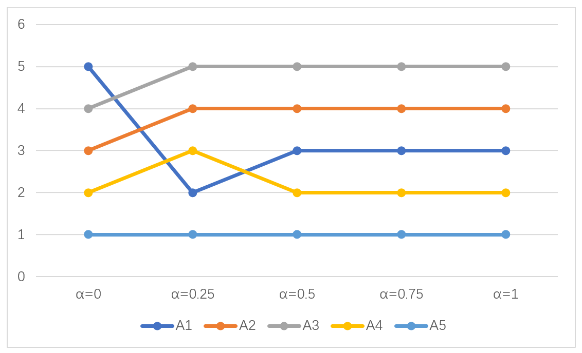
In this section, two forms of sensitivity assessments were conducted: (1) Changing the weight preference coefficient α. (2) Modifying the prospect theory parameters k, τ, and η.
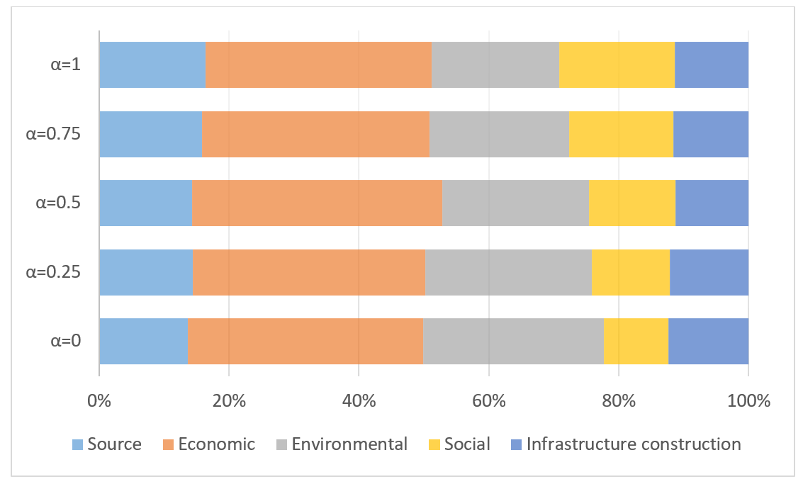
6.1.1. Changing the Weight Preference Coefficient
The order of alternatives is affected by the weightings of the criteria, so it is essential to examine how changes in the indicator weight preference coefficient affect the results. This paper selects α = 0, α = 0.25, α = 0.75, and α = 1, and Figure 4 shows the weights of key criteria. As α increases from 0 to 1: The weight proportion of resource indicators shows an upward trend, indicating that the more subjective weights are favored, the higher the weight of resource indicators. The weight proportion of economic indicators decreases with increasing α, showing a higher proportion at α = 0 and gradually declining as the influence of subjective weights increases. The weight proportion of environmental indicators remains relatively stable, with small variation ranges under different α values. The weight proportion of social indicators decreases slightly with increasing α, but the variation is minimal. The weight proportion of infrastructure construction indicators shows a rising trend as α increases from 0 to 1, but the variation range is smaller than that of resource indicators. This indicates that resource and economic indicators are more sensitive to the weight preference coefficient α, with their weight proportions fluctuating significantly with changes in α. Environmental and social indicators exhibit lower sensitivity with relatively stable weights, while infrastructure construction indicators show moderate sensitivity, though less pronounced than resource and economic indicators.
The rankings of alternatives based on varying weight preference coefficients are illustrated in Figure 5. It can be observed that A1 is highly sensitive to the weight preference coefficient α, with its ranking fluctuating significantly as α changes. A3 and A4 also exhibit high sensitivity, with their rankings rising as subjective weights increase. A2 shows lower sensitivity, while A5 demonstrates excellent stability, remaining unaffected by changes in the weight preference coefficient and consistently being the optimal investment choice. In investment decision-making: If greater reliance is placed on objective data, A1 may be a preferable choice. If subjective judgment is prioritized, A3 and A4 show more potential. However, A5 remains a reliable fallback option that consistently performs well.
6.1.2. Modifying Prospect Theory Parameters
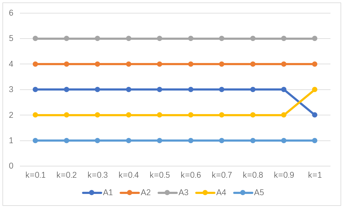
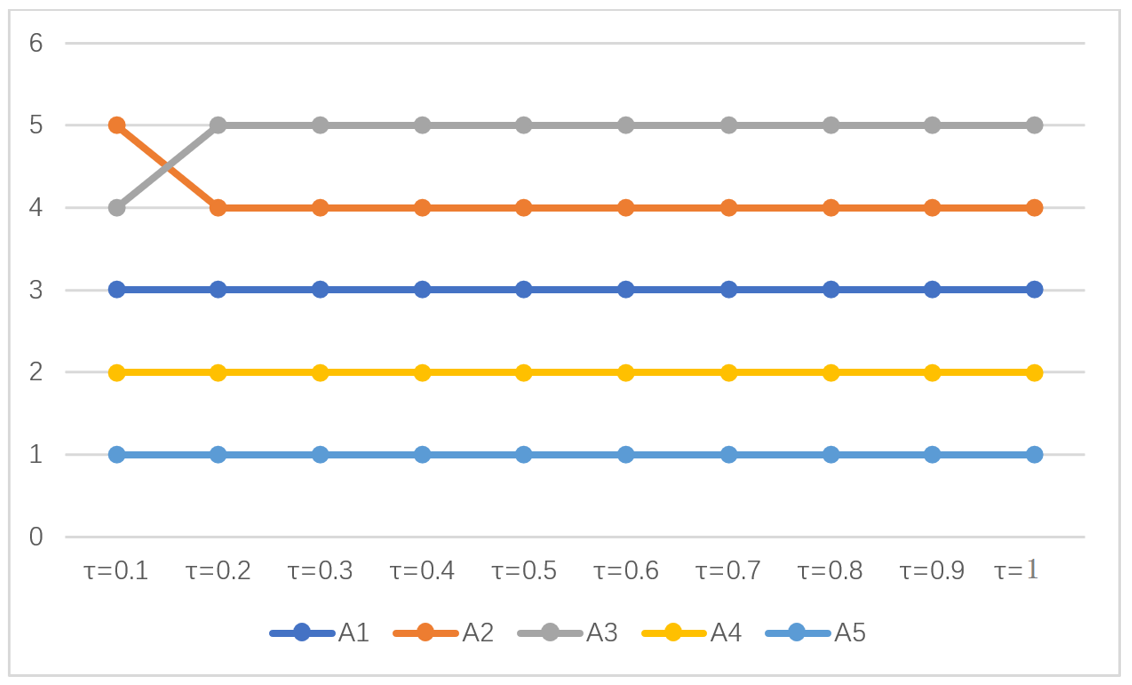
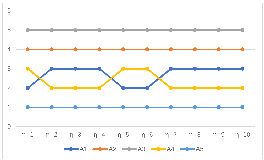
Prospect theory is a framework used to understand how people make choices under uncertainty, particularly when faced with potential gains or losses. When applying prospect theory, it’s crucial to conduct sensitivity analysis on the parameters of the value function, as these parameters reflect the decision-makers’ preferences. In this section, three different scenarios were created by modifying prospect parameters: (1) Sorting parameter k from 0 to 1; (2) Sorting parameter τ from 0 to 1; (3) Sorting parameter η from 0 to 1. Figure 6, Figure 7 and Figure 8 show the rankings of alternatives under the three scenarios.
When k ≤ 0.9, the rankings of alternatives A3, A2, and A5 remain relatively stable. When k ≥ 0.9, the rankings of A1 and A4 change, with A4 surpassing A1. This indicates that when k is small, the alternative rankings are relatively stable, while A1 and A4 become more sensitive to k and their rankings shift as k increases beyond a certain threshold.
For different τ values, the rankings of A1, A3, A4, and A5 are relatively stable across most intervals (τ ≠ 0.1, 0.2), whereas A2 and A3 swap rankings at τ = 0.1 and 0.2. Rankings change only when 0.1 ≤ τ ≤ 0.2, remaining stable otherwise. This suggests that τ significantly impacts the rankings of A2 and A3 within specific intervals, while most alternatives show low sensitivity to τ changes overall.
The parameter η significantly affects alternative rankings. When η ≤ 4, the rankings of A1 and A4 fluctuate frequently; when η > 4, the rankings gradually stabilize. A2 and A3 maintain stable rankings throughout the η variation range. The analysis shows that small η values lead to significant ranking fluctuations, reflecting strong impacts of decision-makers’ preferences on alternative selection, while large η values stabilize rankings, indicating weakened preference impacts.
Among these parameters, k and τ alter rankings of specific alternatives within limited intervals, whereas η directly and most profoundly influences rankings by reflecting decision preferences. Accurately determining the η value is crucial for making rational decisions in the decision-making process.
6.2. Comparative Analysis
To analyze how different ranking methods affect the optimal investment plan for MECS, this study compares the proposed approach with TOPSIS, VIKOR, MABAC, and PROMETHEE. Table 16 displays the results of the four methods.
MCDM methods vary in their modeling logic. TOPSIS and VIKOR rank alternatives based on their proximity to the ideal solution, while MABAC assesses dominance by considering relative positions within the boundary approximate area. PROMETHEE builds a preference matrix with criterion-based inter-alternative preference functions and ranks alternatives via net outranking flow. However, as shown in Table 16, there is a remarkable consistency in the priority rankings identified by the proposed method, TOPSIS, and VIKOR. All three methods yield the same ranking: “A5 > A4 > A1 > A2 > A3”. This consistency indicates that across methods, key performance disparities among alternatives are captured in core evaluation dimensions, such as indicator weight allocation and trade-offs between benefit-type and cost-type indicators, validating the comprehensive advantage of A5 and relative disadvantage of A3.
Conversely, PROMETHEE and MABAC, however, show a local rank reversal of A1 and A4 with the sequence “A5 > A1 > A4 > A2 > A3”, due to different algorithmic logics: PROMETHEE, an outranking method, amplifies local advantages of individual high-weight criteria, and A1’s superiority in infrastructure indicators such as C13 and C14 is weighted and highlighted by its calculation; MABAC, a boundary approximation method, is highly sensitive to local indicator characteristics, and A1’s locally optimal performance in infrastructure indicators makes its distance to the ideal-anti-ideal boundary area better, thus outranking A4. In contrast, TOPSIS, VIKOR, and the proposed model all focus on the global comprehensive performance of alternatives and emphasize the balance of each criterion. A4 has better comprehensive performance in core criteria such as C1 and C6, so it consistently ranks higher than A1. All methods identify A5 as the optimal and A3 as the least preferred alternative, which fully verifies the reliability of the decision results of the proposed model.
In summary, the proposed model is highly consistent with TOPSIS, VIKOR, PROMETHEE, and MABAC in core decision conclusions, all verifying A5 as the optimal alternative, which fully reflects the reliability of its results. Its incremental value is remarkable: it avoids the over-amplification of local indicator advantages by PROMETHEE and excessive sensitivity to local features by MABAC, and makes up for the defects of traditional methods in ignoring decision-makers’ risk perception and one-sided weighting logic. Integrating Pythagorean fuzzy sets, subjective-objective combined weighting, and prospect theory-GLDS, the model can accurately handle fuzzy uncertainty, balance expert experience and objective data scientifically, integrate risk psychology to fit actual decision-making, and balance the global performance of alternatives and multi-criterion equilibrium, providing a more practically valuable methodological framework for MECS investment decision-making under high uncertainty.
Table 16. Ranking results of different MCDM methods.
|
Methods |
Ranking |
|---|---|
|
The Method |
A5 > A4 > A1 > A2 > A3 |
|
TOPSIS |
A5 > A4 > A1 > A2 > A3 |
|
VIKOR |
A5 > A4 > A1 > A2 > A3 |
|
MABAC |
A5 > A1 > A4 > A2 > A3 |
|
PROMETHEE |
A5 > A1 > A4 > A2 > A3 |
7. Conclusions
Against the backdrop of existing MCDM models’ limitations in energy investment—insufficient fuzzy information processing, neglect of risk perception, and rigid weighting mechanisms—this study proposes a targeted MECS investment decision framework integrating Pythagorean fuzzy sets, prospect theory, and FWZIC-WENSLO combined weighting. Different from existing literature that either applies MCDM models to single-energy investment or conducts partial method improvement, this study achieves systematic optimization of MCDM models for MECS’s characteristics: (1) The universal five-dimensional evaluation system addresses the lack of cross-system comparability in existing energy investment research; (2) PFS and Choquet integral enhance the accuracy of fuzzy information processing and energy compatibility quantification; (3) FWZIC-WENSLO combined weighting balances subjective experience and objective data, overcoming the one-sidedness of single weighting methods; (4) The prospect-GLDS integration reflects risk perception, making decision-making more in line with actual energy investment behavior. Empirical validation in Hebei Province confirms the framework’s applicability, providing a new methodological reference for energy investment decision-making under high uncertainty.
Through the synergistic innovation of the index system, weight fusion mechanism, and risk perception ranking model, this framework provides a scientific, universal, and practical decision support tool for MECS projects, contributing significantly to theoretical development and practical application in energy system optimization and sustainable development.
Despite the theoretical and practical contributions of this study, several limitations should be acknowledged. First, the proposed framework relies heavily on expert judgments, which may introduce subjectivity and potential bias, even though measures such as trust-based weighting and fuzzy logic were employed to mitigate this issue. Second, the current model assumes static criteria weights and does not account for dynamic changes in the energy market or policy environment over time. Third, the case study is limited to five projects in Hebei Province, China, which may restrict the generalizability of the findings to other regions or countries with different energy structures and regulatory frameworks.
Future research could address these limitations by developing a dynamic multi-stage decision-making model that incorporates time-series data and real-time updates of criteria weights. In addition, integrating machine learning techniques to learn from historical project data could enhance the objectivity and adaptability of the evaluation process. Furthermore, the framework could be extended to incorporate stakeholder consensus mechanisms to better reflect group decision-making dynamics. Finally, cross-regional comparative studies involving different countries or climate zones would help validate and generalize the proposed framework, thereby enhancing its applicability in diverse energy planning contexts.
Statement of the Use of Generative AI and AI-Assisted Technologies in the Writing Process
During the preparation of this manuscript, the authors used generative AI tools to assist with language polishing and format organization. After using the tool/service, the authors reviewed and edited the content as needed and take full responsibility for the content of the published article.
Author Contributions
Q.M.: Supervision, Project administration, Investigation, Conceptualization. F.D.: Writing—review & editing, Writing—original draft, Visualization, Validation, Supervision, Software, Resources, Methodology, Formal analysis, Data curation. X.Y.: Validation, Supervision, Conceptualization, Writing—review & editing. G.D.: Validation, Supervision, Writing—review & editing.
Ethics Statement
Not applicable.
Informed Consent Statement
Not applicable.
Data Availability Statement
The data that support the findings of this study are available from the corresponding author upon reasonable request.
Funding
This research received no external funding.
Declaration of Competing Interest
The authors declare that they have no known competing financial interests or personal relationships that could have appeared to influence the work reported in this paper.
References
- Hua H, Du C, Chen X, Kong H, Li K, Liu Z, et al. Optimal dispatch of multiple interconnected-integrated energy systems considering multi-energy interaction and aggregated demand response for multiple stakeholders. Appl. Energy 2024, 376, 124256. DOI:10.1016/j.apenergy.2024.124256 [Google Scholar]
- Quizhpe K, Arévalo P, Ochoa-Correa D, Villa-Ávila E. Optimizing Microgrid Planning for Renewable Integration in Power Systems: A Comprehensive Review. Electronics 2024, 13, 3620. DOI:10.3390/electronics13183620 [Google Scholar]
- Wang J, Cui Y, Liu Z, Zeng L, Yue C, Agbodjan YS. Multi-energy complementary integrated energy system optimization with electric vehicle participation considering uncertainties. Energy 2024, 309, 133109. DOI:10.1016/j.energy.2024.133109 [Google Scholar]
- Wu Y, Wu C, Zhou J, He F, Xu C, Zhang B, et al. An investment decision framework for photovoltaic power coupling hydrogen storage project based on a mixed evaluation method under intuitionistic fuzzy environment. J. Energy Storage 2020, 30, 101601. DOI:10.1016/j.est.2020.101601 [Google Scholar]
- Liu Z, Cui Y, Wang J, Yue C, Agbodjan YS, Yang Y. Multi-objective optimization of multi-energy complementary integrated energy systems considering load prediction and renewable energy production uncertainties. Energy 2022, 254, 124399. DOI:10.1016/j.energy.2022.124399 [Google Scholar]
- Lin J, Gu Y, Wang Z, Zhao Z, Zhu P. Operational characteristics of an integrated island energy system based on multi-energy complementarity. Renew. Energy 2024, 230, 120890. DOI:10.1016/j.renene.2024.120890 [Google Scholar]
- Wei D, Zhang Y, Li J, Yuan S, Geng Y, Cheng Y, et al. Research and Application of Multi-energy Complementary Comprehensive Energy Distributed Measurement and Control System. IOP Conf. Ser. Earth Environ. Sci. 2020, 510, 022036. DOI:10.1088/1755-1315/510/2/022036 [Google Scholar]
- Arévalo P, Cano A, Jurado F. Large-scale integration of renewable energies by 2050 through demand prediction with ANFIS, Ecuador case study. Energy 2024, 286, 129446. DOI:10.1016/j.energy.2023.129446 [Google Scholar]
- Lin X, Zhang N, Zhong W, Kong F, Cong F. Regional integrated energy system long-term planning optimization based on multi-energy complementarity quantification. J. Build. Eng. 2023, 68, 106046. DOI:10.1016/j.jobe.2023.106046 [Google Scholar]
- Liu C, Wang H, Wang Z, Liu Z, Tang Y, Yang S. Research on life cycle low carbon optimization method of multi-energy complementary distributed energy system: A review. J. Clean. Prod. 2022, 336, 130380. DOI:10.1016/j.jclepro.2022.130380 [Google Scholar]
- Zhao G, Yu C, Huang H, Yu Y, Zou L, Mo L. Optimization Scheduling of Hydro–Wind–Solar Multi-Energy Complementary Systems Based on an Improved Enterprise Development Algorithm. Sustainability 2025, 17, 2691. DOI:10.3390/su17062691 [Google Scholar]
- Jing Z, Wang Y, Chang J, Wang X, Guo A, Meng X. Hydro-wind-PV-storage complementary operation based on a multivariate 3D power generation database considering comprehensive utilization tasks of cascade hydropower stations in the river basin. Energy 2025, 322, 135672. DOI:10.1016/j.energy.2025.135672 [Google Scholar]
- Ma Y, Yu L, Zhang G, Lu Z, Wu J. Source-load uncertainty-based multi-objective multi-energy complementary optimal scheduling. Renew. Energy 2023, 219, 119483. DOI:10.1016/j.renene.2023.119483 [Google Scholar]
- Wang Y, Gao J, Wei L, Wu H, Zhao S. Geographic information system-based multi-criteria decision-making analysis for investment assessment of wind-photovoltaic-shared energy storage power stations: a case study of Shanxi Province. Environ. Sci. Pollut. Res. Int. 2024, 31, 22604–22629. DOI:10.1007/s11356-024-32123-5 [Google Scholar]
- Li W, Dong F, Shi M, Wang X, Ji Z. Multi-attribute decision-making research on investment suitability assessment of hydropower-wind-photovoltaic-storage complementary system based on dynamic social network. Energy Convers. Manag. 2024, 307, 118358. DOI:10.1016/j.enconman.2024.118358 [Google Scholar]
- Guo F, Gao J, Liu H, He P. A hybrid fuzzy investment assessment framework for offshore wind-photovoltaic-hydrogen storage project. J. Energy Storage 2022, 45, 103757. DOI:10.1016/j.est.2021.103757 [Google Scholar]
- Arévalo P, Benavides D, Lata‐García J, Jurado F. Techno-economic evaluation of renewable energy systems combining PV-WT-HKT sources: Effects of energy management under Ecuadorian conditions. Int. Trans. Electr. Energy Syst. 2020, 30, e12567. DOI:10.1002/2050-7038.12567 [Google Scholar]
- Mao Q, Fan J, Imtiaz S, Mudassir Munir H, Alsenani TR, Alharbi M. Prioritization of renewable energy for offshore ship charging stations based on intuitionistic fuzzy GLDS method: A case of China. Heliyon 2024, 10, e36530. DOI:10.1016/j.heliyon.2024.e36530 [Google Scholar]
- Ziadi K, Barakat A, Elaloui A, Ouayah M, Namous M. Prioritization of the Tassaoute Watershed (Morocco) for soil erosion using analytical hierarchy process (AHP) and geospatial techniques. Geosyst. Geoenviron. 2025, 4, 100389. DOI:10.1016/j.geogeo.2025.100389 [Google Scholar]
- Oraya AF, Canseco-Tuñacao HA, Luciano R, Patadlas A, Baguio I, Aro JL, et al. An Integrated Multi-criteria Sorting Methodology withq -Rung Orthopair Fuzzy Sets for Evaluating the Impacts of Delays on Residential Construction Projects. Axioms 2023, 12, 735. DOI:10.3390/axioms12080735 [Google Scholar]
- Ogundoyin SO, Kamil IA. An integrated Fuzzy-BWM, Fuzzy-LBWA and V-Fuzzy-CoCoSo-LD model for gateway selection in fog-bolstered Internet of Things. Appl. Soft Comput. J. 2023, 143, 110393. DOI:10.1016/j.asoc.2023.110393 [Google Scholar]
- Feng X, Zibibula M, Wei C. Evaluation of dynamic technological innovation capability in high-tech enterprises based on pythagorean fuzzy LBWA and MULTIMOORA. J. Intell. Fuzzy Syst. 2023, 44, 9143–9165. DOI:10.3233/JIFS-222965 [Google Scholar]
- Ara MA, Sultana M, Mou SS, Sakib MSA, Shabur MA. Assessing the obstacles to green supply chain management in Bangladesh’s footwear industry using SWARA and ISM-MICMAC methods. Discov. Sustain. 2024, 5, 463. DOI:10.1007/s43621-024-00657-w [Google Scholar]
- Sithi SS, Ara MA, Dhrubo AT, Rony AH, Shabur MA. Sustainable supplier selection in the textile industry using triple bottom line and SWARA-TOPSIS approaches. Discov. Sustain. 2025, 6, 344. DOI:10.1007/s43621-025-01206-9 [Google Scholar]
- Yazdanirad S, Shakerian M, Khoshakhlagh AH, Rafiei A, Mousavi SM. Identification, classification, and prioritization of the main risk factors of work-related musculoskeletal disorders using the hybrid SWARA-PROMETHEE method. WORK A J. Prev. Assess. Rehabil. 2025, 81, 3151–3161. DOI:10.1177/10519815251324004 [Google Scholar]
- Derse O. Prioritizing solutions of green Reverse logistics barriers with Fuzzy DEMATEL—FUCOM—SWARA methods. Ecol. Indic. 2024, 165, 112198. DOI:10.1016/j.ecolind.2024.112198 [Google Scholar]
- Gan Y, Zheng C, Chu B, Li J, Zhang Y, Jia Y. Research on the risk assessment of the power grid enterprises’ agency power purchase business in China: A hybrid multi-attribute decision-making framework based on FUCOM-F and GRA-MARCOS. Front. Energy Res. 2024, 12, 1376531. DOI:10.3389/fenrg.2024.1376531 [Google Scholar]
- Hatice Gökler S. Optimal site selection for electric vehicle charging stations: Analysis with hybrid FUCOM and geographic information systems. Energy 2024, 307, 132659. DOI:10.1016/j.energy.2024.132659 [Google Scholar]
- Albahri AS, Hamid RA, Alzubaidi L, Homod RZ, Zidan KA, Mubark H, et al. Prioritizing complex health levels beyond autism triage using fuzzy multi-criteria decision-making. Complex Intell. Syst. 2024, 10, 6159–6188. DOI:10.1007/s40747-024-01432-0 [Google Scholar]
- Taha Aljburi M, Albahri AS, Albahri OS, Alamoodi AH, Mahdi Mohammed S, Deveci M, et al. Exploring decision-making techniques for evaluation and benchmarking of energy system integration frameworks for achieving a sustainable energy future. Energy Strategy Rev. 2024, 51, 101251. DOI:10.1016/j.esr.2023.101251 [Google Scholar]
- Xiao L, Fang T, Huang G, Deveci M. An integrated design concept evaluation method based on fuzzy weighted zero inconsistency and combined compromise solution considering inherent uncertainties. Adv. Eng. Inform. 2025, 65, 103097. DOI:10.1016/j.aei.2024.103097 [Google Scholar]
- Hantoobi SA, Zaidan AA, Ibrahim HA, Qahtan S, Deveci M, Isik S, et al. Security modules of delegation methods in mobile cloud computing using probabilistic interval neutrosophic hesitant fuzzy set based decision-making model. Appl. Soft Comput. 2025, 175, 113089. DOI:10.1016/j.asoc.2025.113089 [Google Scholar]
- Al-Hchaim AAJ, Muhsen YR, Gwad WH, Alkayal ES, Ogaili RRNA, Alyasseri ZAA, et al. Prioritizing Network-On-Chip Routers for Countermeasure Techniques against Flooding Denial-of-Service Attacks: A Fuzzy Multi-Criteria Decision-Making Approach. Comput. Model. Eng. Sci. 2025, 142, 2661–2689. DOI:10.32604/cmes.2025.061318 [Google Scholar]
- Bilquise G, Ibrahim S. Integrating ARAS with PyFWZIC to evaluate and benchmark patient-facing genetic services digital tools. Neural Comput. Appl. 2024, 36, 18201–18222. DOI:10.1007/s00521-024-10153-x [Google Scholar]
- Zhu Y, Guo Y, Chen Y, Ma J, Zhang D. Factors Influencing Carbon Emission and Low-Carbon Development Levels in Shandong Province: Method Analysis Based on Improved Random Forest Partial Least Squares Structural Equation Model and Entropy Weight Method. Sustainability 2024, 16, 8488. DOI:10.3390/su16198488 [Google Scholar]
- Sun L, Chen B, Zhou Q, Zhao D. Multi-objective optimization of wire cutting process parameters for Ti-6Al-4V alloy is performed using NSGA-II and EWM-TOPSIS optimized artificial neural network. Proc. Inst. Mech. Eng. Part C J. Mech. Eng. Sci. 2025, 239, 3772–3789. DOI:10.1177/09544062251315035 [Google Scholar]
- Zhang Q, Ge D, Mi S, Lu Q. An eco-friendly and effective method for isolating essential oil from fresh Kaempferia galanga L.: Process optimization based on entropy weight method and response surface methodology. Sustain. Chem. Pharm. 2025, 45, 102042. DOI:10.1016/j.scp.2025.102042 [Google Scholar]
- Salaj, Kumari M. A multi-criteria approach to blockchain in supply chain management assessment: Entropy-CRITIC weight method and MCDM for enhanced decision support. Int. J. Syst. Assur. Eng. Manag. 2025, 16, 1830–1843. DOI:10.1007/s13198-025-02764-x [Google Scholar]
- Shahzadi G, Sarwar M, Riasat A. Hybrid decision making model for COVID-19 effects: A (p, q)-rung orthopair fuzzy integrated CRITIC-DEMATEL-MABAC approach. Afr. Mat. 2025, 36, 109. DOI:10.1007/s13370-025-01330-9 [Google Scholar]
- Song S, Meng A, Xiao L, Tan Z, Zou P, Yin H, et al. Research on data augmentation and synthetic sample quantity uncertainty in few-shot wind power prediction based on the adaptive CRITIC-HLICRVFL method. Renew. Energy 2025, 252, 123527. DOI:10.1016/j.renene.2025.123527 [Google Scholar]
- Liang X. MEREC-Based Combined Framework for Multiple-Attribute Group Decision-Making in Probabilistic Linguistic Environment: Applications to Technology Finance Development Efficiency Evaluation. Int. J. Decis. Support Syst. Technol. 2024, 16, 1–18. DOI:10.4018/IJDSST.361906 [Google Scholar]
- Kou G, Aydın FB, Eti S, Yüksel S, Dinçer H. A novel Spherical fuzzy MEREC-ARAS decision framework for optimizing innovation-driven investment strategies in energy systems. Energy Strategy Rev. 2025, 59, 101771. DOI:10.1016/j.esr.2025.101771 [Google Scholar]
- Seikh MR, Chatterjee P. Sustainable strategies for electric vehicle adoption: A confidence level-based interval-valued spherical fuzzy MEREC-VIKOR approach. Inf. Sci. 2025, 699, 121814. DOI:10.1016/j.ins.2024.121814 [Google Scholar]
- Riaz M, Qamar F, Tariq S, Alsager K. AI-Driven LOPCOW-AROMAN Framework and Topological Data Analysis Using Circular Intuitionistic Fuzzy Information: Healthcare Supply Chain Innovation. Mathematics 2024, 12, 3593. DOI:10.3390/math12223593 [Google Scholar]
- Dhruva S, Krishankumar R, Zavadskas EK, Ravichandran KS, Gandomi AH. Selection of Suitable Cloud Vendors for Health Centre: A Personalized Decision Framework with Fermatean Fuzzy Set, LOPCOW, and CoCoSo. Informatica 2024, 35, 65–98. DOI:10.15388/23-INFOR537 [Google Scholar]
- Ecer F, Tanrıverdi G, Yaşar M, Görçün ÖF. Sustainable aviation fuel supplier evaluation for airlines through LOPCOW and MARCOS approaches with interval-valued fuzzy neutrosophic information. J. Air Transp. Manag. 2025, 123, 102705. DOI:10.1016/j.jairtraman.2024.102705 [Google Scholar]
- Pamucar D, Ecer F, Gligorić Z, Gligorić M, Deveci M. A Novel WENSLO and ALWAS Multi-criteria Methodology and Its Application to Green Growth Performance Evaluation. IEEE Trans. Eng. Manag. 2024, 71, 9510–9525. DOI:10.1109/TEM.2023.3321697 [Google Scholar]
- Kara K, Yalçın GC, Akagün Ergin E, Simic V, Pamucar D. A neutrosophic WENSLO-ARLON model for measuring sustainable brand equity performance. Socio-Econ. Plan. Sci. 2024, 94, 101918. DOI:10.1016/j.seps.2024.101918 [Google Scholar]
- Kara K, Akagün Ergin E, Cihan Yalçın G, Çelik T, Deveci M, Kadry S. Sustainable brand logo selection using an AI-Supported PF-WENSLO-ARLON hybrid method. Expert Syst. Appl. 2025, 260, 125382. DOI:10.1016/j.eswa.2024.125382 [Google Scholar]
- Sánchez-Lozano JM, Ramos-Escudero A, Gil-García IC, García-Cascales MS, Molina-García A. A GIS-based offshore wind site selection model using fuzzy multi-criteria decision-making with application to the case of the Gulf of Maine. Expert Syst. Appl. 2022, 210, 118371. DOI:10.1016/j.eswa.2022.118371 [Google Scholar]
- Baral SP, Parida PK, Sahoo D. Fuzzy TOPSIS technique for multi-criteria group decision-making: A study of crude oil price. Results Control Optim. 2025, 19, 100565. DOI:10.1016/j.rico.2025.100565 [Google Scholar]
- Ding Y, Jing X, Xie F, Chen S, Zhang C, Zhao G, et al. TOPSIS analysis and failure mechanism of low-velocity impact behavior of S-glass/aramid fiber reinforced hybrid composite laminates. Thin-Walled Struct. 2025, 215, 113489. DOI:10.1016/j.tws.2025.113489 [Google Scholar]
- Hendiani S, Torkayesh AE, Venghaus S, Walther G. Leading the green charge: A novel type-2 fuzzy VIKOR method applied to eco-conscious freight transport. Expert Syst. Appl. 2025, 285, 128082. DOI:10.1016/j.eswa.2025.128082 [Google Scholar]
- Ma Y, Zhi G, Alfarraj O, Alblehai F, Yu J. Hybrid AHP-VIKOR methodology for multi-criteria decision-making in marine renewable energy systems: Optimizing DC-DC buck converters for sustainable offshore applications. Mar. Pollut. Bull. 2025, 214, 117809. DOI:10.1016/j.marpolbul.2025.117809 [Google Scholar]
- Debnath K, Roy SK, Deveci M, Tomášková H. Integrated MADM approach based on extended MABAC method with Aczel–Alsina generalized weighted Bonferroni mean operator. Artif. Intell. Rev. 2024, 58, 27. DOI:10.1007/s10462-024-10980-3 [Google Scholar]
- Ahmmad J, Al-Dayel OA, Khan MA, Mahmood T. AI-assisted technology optimization in disability support systems using fuzzy rough MABAC decision-making. Sci. Rep. 2025, 15, 18335. DOI:10.1038/s41598-025-02362-8 [Google Scholar]
- Aydin M, Camliyurt G, Gul M, Sezer SI, Celik E, Akyuz E. An interval type-2 fuzzy MARCOS modelling to assess performance effectiveness of survival craft on cargo ship. Ocean Eng. 2025, 326, 120899. DOI:10.1016/j.oceaneng.2025.120899 [Google Scholar]
- Santhiya P, Das A. A novel bipolar hexagonal fuzzy MARCOS method for warehouse selection to e-waste recycling in a mass quantity. Expert Syst. Appl. 2025, 283, 127667. DOI:10.1016/j.eswa.2025.127667 [Google Scholar]
- Wang X, Gou X, Xu Z. A continuous interval-valued double hierarchy linguistic GLDS method and its application in performance evaluation of bus companies. Appl. Intell. 2021, 52, 4511–4526. DOI:10.1007/s10489-021-02581-2 [Google Scholar]
- Wu X, Liao H. A consensus-based probabilistic linguistic gained and lost dominance score method. Eur. J. Oper. Res. 2019, 272, 1017–1027. DOI:10.1016/j.ejor.2018.07.044 [Google Scholar]
- Zhang Z, Liao H. Emergency response determination by a choquet-integral-based hybrid gained and lost dominance score method with incomplete attribute weight information. Transform. Bus. Econ. 2022, 21, 290–312. Available online: https://search.ebscohost.com/login.aspx?direct=true&profile=ehost&scope=site&authtype=crawler&jrnl=16484460&AN=156137726&h=iWn%2FkzNq1o568Dk47VHXAzdXuQtI4yY9JXw5n%2FOrpbja13CTTPYsoraWCERK1%2FzUo3XrSvSlP8LH2RfdSsFPZw%3D%3D&crl=c (accessed on 27 March 2026).
- Hong N, Wang X, Xu Z. Probabilistic reliable linguistic term sets applied to investment project selection with the gained and lost dominance score method. Int. J. Mach. Learn. Cybern. 2021, 12, 2163–2183. DOI:10.1007/s13042-021-01299-4 [Google Scholar]
- Liang X, Wu X, Liao H. A gained and lost dominance score II method for modelling group uncertainty: Case study of site selection of electric vehicle charging stations. J. Clean. Prod. 2020, 262, 121239. DOI:10.1016/j.jclepro.2020.121239 [Google Scholar]
- Ming Y, Luo L, Wu X, Liao H, Lev B, Jiang L. Managing patient satisfaction in a blood-collection room by the probabilistic linguistic gained and lost dominance score method integrated with the best-worst method. Comput. Ind. Eng. 2020, 145, 106547. DOI:10.1016/j.cie.2020.106547 [Google Scholar]
- Jiang J, Liu X, Wang W, Deveci M. Assessing the impact of healthcare service risks on healthcare demand under evolving economic and social structures: An improved GLDS decision making method considering risk attitudes. Struct. Change Econ. Dyn. 2023, 67, 459–479. DOI:10.1016/j.strueco.2023.09.002 [Google Scholar]
- Wu M, Ma S, Fan J. A spherical Z-number multi-attribute group decision making model based on the prospect theory and GLDS method. Complex Intell. Syst. 2024, 10, 8501–8524. DOI:10.1007/s40747-024-01552-7 [Google Scholar]
- Zhan M, Li YL. Risk evaluation of submarine pipelines using improved FMEA model based on social network analysis and extended GLDS method under a linguistic Z-number preference relation environment. J. Loss Prev. Process Ind. 2025, 96, 105611. DOI:10.1016/j.jlp.2025.105611 [Google Scholar]
- Tian G, Chen X, Chen C, Yang Y, Li J, Zhang Y. Multi-scenario investment forecast of new energy projects based on multiple linear regression and comprehensive evaluation model of differentiated project priorities. Heliyon 2024, 10, e23771. DOI:10.1016/j.heliyon.2023.e23771 [Google Scholar]
- Yager RR. Pythagorean Membership Grades in Multi-criteria Decision Making. IEEE Trans. Fuzzy Syst. 2014, 22, 958–965. DOI:10.1109/TFUZZ.2013.2278989 [Google Scholar]
- Zhang X, Xu Z. Extension of TOPSIS to Multiple Criteria Decision Making with Pythagorean Fuzzy Sets. Int. J. Intell. Syst. 2014, 29, 1061–1078. DOI:10.1002/int.21676 [Google Scholar]
- Yager RR, Abbasov AM. Pythagorean Membership Grades, Complex Numbers, and Decision Making. Int. J. Intell. Syst. 2013, 28, 436–452. DOI:10.1002/int.21584 [Google Scholar]
- Wang J, An N. Research on Evaluation Method of Green Suppliers Under Pythagorean Fuzzy Environment. Sustainability 2024, 16, 9124. DOI:10.3390/su16209124 [Google Scholar]
- Liang D, Xu Z, Liu D, Wu Y. Method for three-way decisions using ideal TOPSIS solutions at Pythagorean fuzzy information. Inf. Sci. 2018, 435, 282–295. DOI:10.1016/j.ins.2018.01.015 [Google Scholar]
- Ortiz Y, Arévalo P, Peña D, Jurado F. Recent Advances in Thermal Management Strategies for Lithium-Ion Batteries: A Comprehensive Review. Batteries 2024, 10, 83. DOI:10.3390/batteries10030083 [Google Scholar]