CFD Investigation of Torque Generation in an Archimedes Screw Hydrokinetic Turbine

CFD Investigation of Torque Generation in an Archimedes Screw Hydrokinetic Turbine

Received: 28 January 2026 Revised: 03 March 2026 Accepted: 24 March 2026 Published: 30 March 2026

© 2026 The authors. This is an open access article under the Creative Commons Attribution 4.0 International License (https://creativecommons.org/licenses/by/4.0/).
1. Introduction
The extraction of renewable energy from low-head and low-velocity water flows has attracted increasing interest in recent years due to the growing demand for decentralized and environmentally sustainable power generation. Hydrokinetic turbines offer a promising solution for harnessing energy from rivers, tidal currents, and irrigation canals without requiring large hydraulic heads or extensive civil infrastructure. Among the technologies being explored for such applications, the Archimedes Screw turbine (AST) has emerged as an attractive option due to its simple geometry, robust construction, and ability to operate effectively in shallow and bidirectional flows.
The Archimedes Screw Turbine (AST) consists of one or more helical blades wrapped around a central shaft and can be installed either horizontally or at an inclination. The turbine extracts kinetic energy from flowing water by generating a pressure difference between the upstream and downstream sides of its blades, producing torque ($$\tau$$) about its axis of rotation. Similar to vertical-axis turbines, the AST can be configured with the generator positioned above the water surface, as shown in Figure 1.
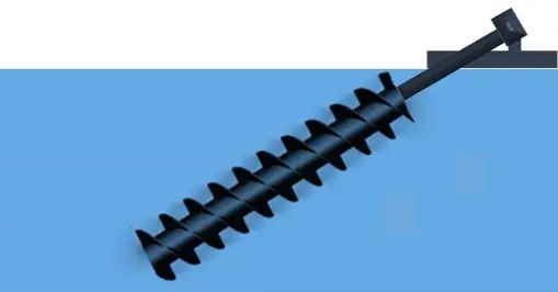
Figure 1. The Archimedes Screw Hydrokinetic Turbine (AST). The water flow can be in either direction.
Unlike conventional axial-flow or crossflow turbines, the AST can operate efficiently at low flow velocities and can tolerate debris and sediment present in natural waterways [1]. These characteristics make it particularly suitable for small-scale hydropower systems and remote energy applications. Although the Archimedes screw has long been used as a pump and, more recently, as a head-driven generator, its use as a hydrokinetic turbine operating primarily from the kinetic energy of the flow remains relatively unexplored.
Previous studies have investigated the performance characteristics of the AST through laboratory experiments. Phillips and Wood [2] measured torque, thrust, and power coefficients for laboratory-scale turbines with different numbers of flights and inclination angles, identifying operating conditions that produced maximum power output. Subsequent particle image velocimetry (PIV) measurements examined the surrounding flow field and applied Proper Orthogonal Decomposition (POD) to identify dominant flow structures [3]. These experiments indicated that the external flow field exhibited minimal cyclic variation and no significant recirculation downstream of the turbine.
Despite these experimental advances, the mechanisms responsible for torque generation in the AST remain insufficiently understood. In particular, the relative contributions of pressure and viscous forces to torque production have not been quantified, and the flow behaviour within the blade passages cannot be directly measured using optical techniques such as PIV. Computational fluid dynamics (CFD), therefore, provides a valuable tool for examining the detailed pressure and velocity fields responsible for turbine loading.
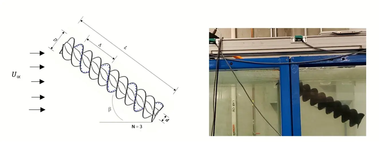
In reference [2], laboratory-scale turbine models with one, two, and three blades (N) were tested to measure torque, thrust, and angular velocity ($$\omega$$) across a range of flow velocities and inclination angles. Two configurations were examined to assess bidirectional operation within a unidirectional water tunnel (Figure 2). Results showed optimal performance at an inclination angle ($$\beta$$) of 30°, with the three-blade turbine achieving a maximum power coefficient ($${C}_{P}$$) of 0.4 at a tip speed ratio ($$\lambda$$) of 0.53 and a free-stream velocity $$\left({U}_{\infty }\right)$$ of 0.45 m/s. For comparable blade counts and tip speed ratios, the first configuration consistently outperformed the second.
 |
|
(a) |
 |
|
(b) |
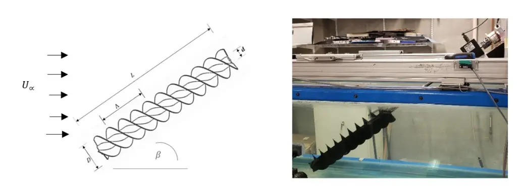
Figure 2. Turbine Orientation and Configurations. (a) First Turbine Configuration. Flow is from left to right. (b) Second Turbine Configuration. Flow is from left to right.
Phase-dependent torque fluctuations observed in [2] indicated periodic variations in the flow field, which were further investigated in [3] using PIV. For both configurations, the measured external wake exhibited no evidence of large-scale flow separation, persistent recirculation, or strongly organized coherent structures. The mean velocity fields were dominated by turbulent mixing, and the Reynolds stress spectra showed broadband characteristics with no dominant peaks at the turbine rotational frequency. POD analysis further indicated that the leading modes captured only a modest fraction of the turbulent kinetic energy, with no low-order mode exhibiting strong phase-locked behaviour. From a modelling perspective, the absence of strong phase-dependent structures in the measured wake supports the use of unsteady Reynolds averaged Navier-Stokes (URANS) approaches for predicting the mean external flow and global wake behaviour of the AST.
A review of the limited literature on the AST and its relation to the Archimedes Screw Generator (ASG) is provided in [2]. The only large-scale AST prototypes reported in the literature are the Delta unit and the Cat 3EC42 deployed by Jupiter Hydro [4]. The Cat 3EC42 comprises two ASTs, each with a diameter of 0.91 m and a length of 2.85 m mounted on an equilateral triangular platform and coupled to 3 kW synchronous permanent magnet generators. Field testing achieved a maximum power coefficient of 0.5 and a maximum torque at a tip speed ratio of 0.5, with the torque coefficient decreasing as the tip speed ratio increased. Zitti et al. [5] conducted experimental and numerical investigations on a small-scale AST model with a diameter of 0.1 m and a length of 0.32 m. They reported average power coefficients of 0.07 from experiments and 0.15 from simulations, concluding that these values are comparable to those of other hydrokinetic turbine types.
The objective of the present study is to use CFD simulations to investigate the hydrodynamic behaviour and torque-generation mechanism of the AST. Building on the experimental configurations examined in [2,3], the simulations quantify the relative contributions of pressure and viscous forces to the torque acting on the turbine blades. The study also examines the temporal characteristics of torque fluctuations and assesses the potential for cavitation under different flow conditions.
The remainder of this paper is organised as follows: Section 2 describes the computational methodology; Section 3 presents results for the two configurations and discusses cavitation; Section 4 summarises the key findings; and Section 5 offers recommendations for future work.
A comprehensive list of mathematical symbols and their definitions is provided in Table 1.
Table 1. List of symbols.
|
Symbol |
Quantity |
Units |
|---|---|---|
|
$$\beta$$ |
Inclination angle |
⸰ |
|
$$D, d$$ |
Turbine outside and inside diameters |
m |
|
$$\tau$$ |
Torque |
Nm |
|
$$T$$ |
Thrust |
N |
|
$$\lambda$$ |
Tip speed ratio |
|
|
$$L$$ |
Turbine length |
m |
|
$$N$$ |
Number of flights/blades |
|
|
$$\mathrm{\Lambda }$$ |
Turbine pitch |
m |
|
$${C}_{P}$$ |
Power coefficient |
|
|
$${C}_{\tau }$$ |
Torque coefficient |
|
|
$${C}_{T}$$ |
Thrust coefficient |
|
|
$${U}_{\infty }$$ |
Free stream velocity |
m/s |
|
$$\omega$$ |
Angular velocity |
rad/s |
|
$$\alpha$$ |
Angular acceleration |
rad/s2 |
|
$$J$$ |
Moment of inertia |
Kg·m2 |
|
$$\rho$$ |
Density |
Kg/m3 |
|
$$\mu$$ |
Dynamic viscosity |
Pa·s |
|
$${P}_{P}$$ |
Pressure coefficient |
|
|
$${P}_{v}$$ |
Saturated water vapour pressure |
Pa |
|
$${P}_{\infty }$$ |
Free stream water pressure |
Pa |
|
$$\sigma$$ |
Cavitation factor |
|
|
$$\xi$$ |
Relative error |
2. Computational Methodology
2.1. Overview
All CFD simulations were performed using ANSYS Fluent 2021 R2 version 21.2. The computational meshes for the stationary and rotating domains were generated using ANSYS Meshing within the same software environment. The simulations were configured and executed in Fluent using the transient pressure-based solver. To replicate the experimental conditions reported in [2,3], the turbine was modelled using a flow-induced rotation approach rather than prescribing a fixed angular velocity. The significant torque ripple guided this choice, observed experimentally, which demonstrated strong cyclic fluctuations in torque output. A steady-state simulation with a constant angular velocity may preclude these unsteady dynamics and may not allow the turbulence model to respond to phase-dependent flow variations. Consequently, the simulations were carried out using a transient URANS framework.
The primary simulation cases examined in this study are listed in Table 2. Cases C1 and C2 were designed to replicate the experimental configurations in [2,3] that gave the maximum power output, while C3 was developed to investigate the onset and likelihood of cavitation. This is why the free-stream velocity is much higher in case C3 (6.5 m/s) than in case C2 (0.45 m/s), which was also the velocity in the measurements. For completeness, Table 2 also shows the steady angular velocity for C1, C2, and C3.
Table 2. Details of CFD Cases.
|
Case |
$${\bm{U}}_{\bm{\infty }}$$ (m/s) |
$$\bm{\omega }$$ (rad/s) |
```latex\bm{\beta }``` |
Configuration |
N |
|---|---|---|---|---|---|
|
C1 |
0.45 |
11.35 |
30° |
First |
3 |
|
C2 |
0.45 |
10.98 |
30° |
Second |
3 |
|
C3 |
6.75 |
198.07 |
30° |
First |
3 |
2.2. Limitations of the Study
Using a flow-induced rotation model required a time-dependent (quasi-steady) URANS approach, which, combined with the large mesh sizes, resulted in substantial computational demands. The available High-Performance Computing (HPC) resources at the University of Calgary restricted the extent of mesh refinement, domain enlargement, and simulation duration possible within the project timeframe.
Free-surface modelling was excluded due to computational cost; incorporating a Volume-of-Fluid (VOF) model would have significantly increased the number of elements and solver time without guaranteeing usable convergence within available HPC limits.
Mesh refinement near solid boundaries was also constrained. Achieving ideal $${y}^{+}$$ values would have required additional prism layers and considerably finer resolution. In this study, $${y}^{+}$$ values between 0 and 10.37 were obtained. Further refinement was not feasible due to the reasons outlined above.
2.3. Computational Domain and Mesh
2.3.1. Sliding Mesh Approach
A sliding mesh (SM) approach was used to capture the unsteady interaction between the stationary water tunnel and the rotating turbine. This method, commonly employed for turbomachinery and rotating flows [6,7], allows separate cell zones to move relative to one another through discrete rotations of the moving domain. The governing equations are modified within the rotating zone to include non-inertial acceleration terms.
2.3.2. Mesh Construction
The stationary and rotating domains were meshed separately:
-
-
Stationary Zone: Polyhedral mesh with 101,768 cells, representing the water tunnel with a cylindrical cutout 0.5 m downstream of the inlet. The size of the stationary domain was equal to the dimensions of the water tunnel used in [2] and has a blockage ratio of 0.187.
-
-
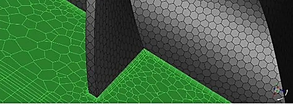
Rotating Zone: Polyhedral mesh with 899,083 cells, created by subtracting the turbine geometry from a cylindrical region identical to the cutout in the stationary mesh.
The two meshes were merged within ANSYS Fluent before case setup. Figure 3 and Figure 4 illustrate the mesh topologies.
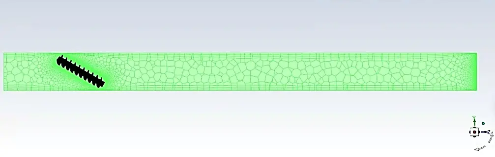
Figure 3. Polyhedral mesh used for the stationary computational domain representing the water tunnel. A cylindrical cutout is introduced to accommodate the rotating mesh region containing the turbine.
 |
|
|
(a) |
|
 |
 |
|
(b) |
(c) |
Figure 4. Mesh of the rotating computational domain containing the turbine and sliding interface. (a) Overall view of the rotating domain mesh. (b) Close-up of the cells at the sliding mesh interface. (c) Close-up of mesh resolution around the turbine blades.
2.3.3. Mesh Quality Assessment
To assess the quality of the computational mesh, standard mesh quality metrics, including skewness and orthogonality, were evaluated in ANSYS Meshing (as outlined in Table 3). These parameters are commonly used to assess mesh reliability and numerical stability in CFD simulations. The skewness values of the mesh were found to be within acceptable limits for polyhedral grids, with a maximum skewness below 0.85 and an average skewness significantly lower. The orthogonal quality values were also satisfactory, with minimum values above 0.15, indicating that the mesh quality was sufficient to ensure stable and accurate numerical solutions.
Table 3. Mesh Quality Metrics.
|
Metric |
Stationary Domain |
Rotating Domain |
|---|---|---|
|
Number of Cells |
101,768 |
899,083 |
|
Maximum Skewness |
~0.83 |
~0.84 |
|
Average Skewness |
~0.22 |
~0.24 |
|
Minimum Orthogonal Quality |
~0.18 |
~0.17 |
|
Average Orthogonal Quality |
~0.82 |
~0.80 |
The acceptable mesh quality metrics, together with the grid convergence study described in Section 2.8, provide confidence that the numerical results are not significantly affected by grid-related errors.
2.4. Turbulence Model
The $$k-\omega$$ SST turbulence model [8,9] was employed in the present simulations. The SST model combines the advantages of the standard $$k-\omega$$ formulation near solid boundaries with the $$k-\epsilon$$ model behaviour in the free stream, providing improved accuracy for flows involving adverse pressure gradients and separation. This hybrid formulation allows the model to resolve near-wall behaviour while maintaining robustness in the outer flow region.
The SST model has been widely used for simulating turbomachinery and hydrokinetic turbines due to its ability to accurately capture boundary-yer development and pressure-driven flow features [10]. Previous numerical investigations of screw-type and hydrokinetic turbines have also successfully applied the SST model to predict turbine performance and flow behaviour [11].
Given the complex geometry of the Archimedes screw turbine and the presence of rotating flow structures within the blade passages, the SST model was considered an appropriate compromise between computational cost and predictive capability. The model is particularly well suited for capturing the pressure gradients and wall-bounded flow behaviour that dominate the torque generation mechanism investigated in this study. As later results show, torque generation is dominated by pressure forces, making accurate prediction of pressure gradients near the blade surfaces particularly important, further supporting the use of the SST formulation.
2.5. Cell Zone and Motion Specification
Flow-Induced Rotation
In the rotating zone, mesh motion was activated, and the rotation axis was defined from the turbine’s mass properties (exported from SolidWorks, which was used for the turbine design). A user-defined function (UDF) was implemented to update the angular velocity ($$\omega$$) at each timestep according to the dynamic balance:
|
```latex\frac{d\omega }{dt}=\alpha = \frac{{\tau }_{n}}{J} \mathrm{\Delta }t``` |
(1) |
which was discretised as:
|
```latex{\omega }_{i+1}- {\omega }_{i}= \frac{{\tau }_{n}}{J} \left({t}_{i+1}- {t}_{i}\right)``` |
(2) |
where $${\omega }_{i}$$ is the angular velocity at time $${t}_{i}$$, $${\tau }_{n}$$ is the net torque acting on the turbine computed within ANSYS Fluent, $$J$$ is the mechanical moment of inertia of the turbine, $$\alpha$$ is the angular acceleration, and $$\mathrm{\Delta }t$$ is the timestep size.
This approach ensures that turbine rotation responds to the instantaneous hydrodynamic forcing. To account for the external torque load (regulating torque/load and resistive/frictional torque in the bearings and instrumentation in the experiments), a resistive torque load of 0.44 Nm was added within the computational setup, such that:
|
```latexJ\alpha = J\frac{d\omega }{dt}= {\tau }_{h}- {\tau }_{c}``` |
(3) |
where $$\alpha$$ is the angular acceleration, obtained by differentiating the values of $$\omega$$, $${\tau }_{h}$$ is the net hydrodynamic torque produced by the turbine, and $${\tau }_{c}$$ is the frictional torque due to the regulating torque/load imposed on the turbine shaft by the magnetic particle brake, as well as friction in the bearings (see experimental set up in [2]). The total torque on the turbine is given by:
|
```latex{\tau }_{n} = {\tau }_{h}- {\tau }_{c}``` |
(4) |
The value of the resistive torque load or Cases C1 and C2 (0.44 Nm) was determined iteratively within ANSYS Fluent while comparing results with experiments until a satisfactory result was obtained. The applied resistive torque represents an effective mean load corresponding to the experimentally measured operating point near maximum power, and allowed the simulations to reach a tip speed ratio that was comparable to the experiment. The present CFD study does not attempt to replicate the full range of experimental brake settings used to generate the complete. $${C}_{P}-\lambda$$ curve. The resistive torque was varied in order to obtain the curve.
2.6. Boundary Conditions
The following conditions were applied:
-
-
Velocity Inlet: Uniform inflow in the positive z-direction
-
-
Pressure Outlet: Zero-gauge pressure
-
-
Walls:
- o
-
No-slip on turbine surfaces, tunnel bottom, and tunnel walls
- o
-
Stationary, zero-shear top surface to approximate a free surface
-
-
Interfaces: Non-conformal sliding and static interfaces between domains
2.7. Solver Settings
-
-
Solver Type: Pressure-based, transient
-
-
Gravity: Negative y-direction
-
-
Pressure–Velocity Coupling: Coupled scheme
-
-
CFL Number: 5 (acceptable for implicit solvers)
-
-
Time Step: $${10}^{-3}$$ s
A fixed time stepping method was used. Initially, a time step size of $${10}^{-4}$$ s was used. This led to very large computational times, and it was impossible to reach or get close to steady-state results with the available computational resources. Using a timestep size of $${10}^{-2}$$ s led to faster progress through the computations but gave questionable results, which were also not consistent.
At the maximum steady-state angular velocity that was studied, approximately 11.38 rad/s, a timestep of $${10}^{-3}$$ s corresponds to a blade rotation of ~0.65°, providing sufficient temporal resolution of the torque oscillations.
Max Iterations per Timestep: 20
To ensure numerical convergence within each timestep, the residuals of the governing equations were monitored during the simulations. For all cases, the residuals for continuity and momentum decreased by at least three orders of magnitude within each timestep. In addition to monitoring residuals, the turbine torque and angular velocity were tracked throughout the simulations to verify that the solution within each timestep was sufficiently converged. Tests with larger iteration counts showed negligible changes in these monitored quantities, indicating that 20 iterations per timestep were sufficient to achieve stable, converged solutions while maintaining a reasonable computational cost. Increasing the maximum number of iterations beyond 20 produced no observable change in the cycle-averaged torque or steady-state angular velocity.
-
-
Initialisation: Standard initialisation from the inlet
-
-
Fluid Properties: Water at 20 °C
- o
-
Density ($$\rho$$) = 103 kg/m3
- o
-
Viscosity ($$\mu$$) = 10−3 Pa·s
2.8. Grid Convergence Study
A grid independence assessment was carried out using Case C1 across four grid levels. Successive meshes used an expansion ratio of 1:4. Grid convergence was evaluated based on a difference of ≤10% in the values of measured parameters between different consecutive mesh sizes. Using the Richardson extrapolation [12], the extrapolated value of $$\tau$$ is:
|
```latex{\tau }_{e} \approx {\tau }_{{m}_{1}}+ \frac{{\tau }_{m1}- {\tau }_{m2}}{{r}^{l}-1}``` |
(5) |
where $$r$$ is the grid refinement ratio, and $$l$$ is the order of the method. $${m}_{1}$$ represents one level of grid refinement, and $${m}_{2}$$ would represent the next level of refinement. The relative error is calculated as:
|
```latex\xi = \frac{|{\tau }_{e}- {\tau }_{m1}|}{{\tau }_{e}}``` |
(6) |
Grid independence was assumed when ($$\xi$$ < 0.1%). Table 4 outlines the details of the cell counts for the grids used in the grid convergence study, and Figure 5 shows the torque and angular velocity evolution for the four grids, demonstrating consistent behaviour across meshes despite the transient nature of the solution. The coarsest grid meeting the convergence criteria was used in subsequent simulations.
Table 4. Grid convergence study cell counts based on Case C1.
|
Tunnel Domain |
Rotating Domain |
Total Cell Count |
$${\bm{C}}_{\bm{P}}$$ |
% Difference |
|---|---|---|---|---|
|
325,931 |
628,330 |
954,261 |
0.831 |
- |
|
414,766 |
977,556 |
1,392,322 |
0.823 |
4.00 |
|
503,937 |
1,335,123 |
1,839,060 |
0.839 |
1.90 |
|
597,865 |
1,706,928 |
2,304,793 |
0.841 |
0.23 |
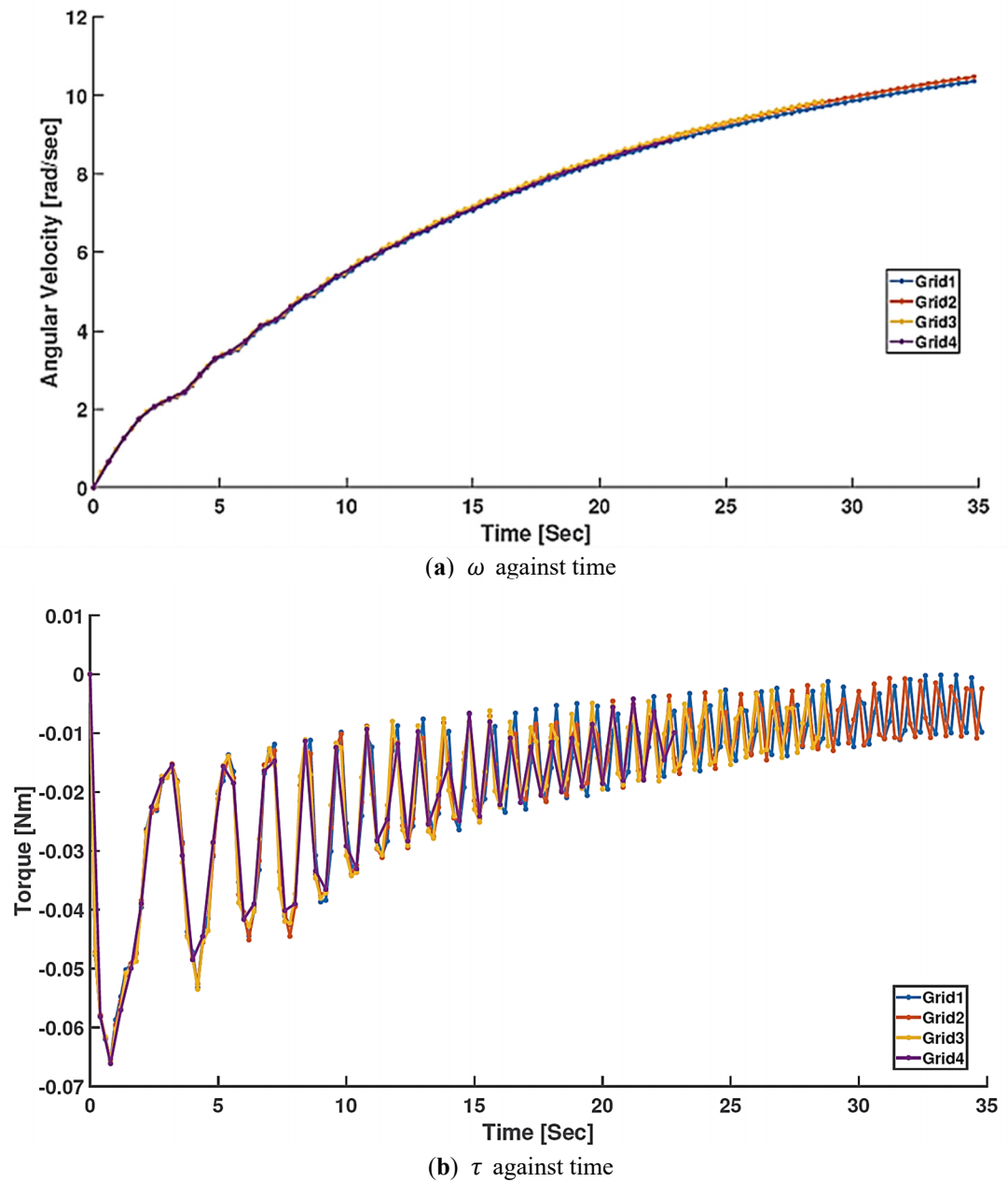
Figure 5. Evolution of turbine response for the four grids used in the grid convergence study for Case C1. (a) Torque as a function of time. (b) Angular velocity as a function of time. The similar behaviour observed for successive meshes indicates grid-independent results.
3. Results
3.1. First Configuration
During the simulation, data were recorded every 300 timesteps. Figure 6 presents the net torque and angular velocity versus time for Case C1 and shows that the torque fluctuations diminish as the turbine approaches steady-state operation. As expected, the angular velocity converges to a constant steady-state value as the torque variation decreases. The agreement between the steady-state angular velocity obtained from CFD and the experimental measurements is addressed later through a comparison of $${C}_{P}$$ and $${C}_{\tau }$$ trends.
The presence of torque ripples indicates that the flow is inherently unsteady. Even if a constant angular velocity is prescribed, the flow may still exhibit cyclic torque variations. However, under such conditions, the turbulence model cannot adequately respond to these cyclic variations, leading to inaccurate predictions. For this reason, flow-induced simulations are necessary for accurately representing the turbine’s behaviour. The ripples were observed to occur once per revolution, rather than once per flight, as reported in the experiments of [2]. Additionally, the torque reaches a maximum at t = 0, suggesting that an AST accelerates rapidly from rest. As the turbine approaches steady state, the cyclic torque oscillations settle to a non-zero cycle-averaged value.
To quantify the magnitude of the cyclic torque variations, two commonly used metrics were evaluated: the torque ripple factor (TRF) and the torque ripple percentage (TRP). These quantities are defined in Equations (7) and (8), respectively, and were computed from the quasi-steady portion of the torque time history after the turbine reached a steady angular velocity:
|
```latex\mathrm{T}\mathrm{R}\mathrm{F}= {\tau }_{\mathrm{m}\mathrm{a}\mathrm{x}}- {\tau }_{\mathrm{m}\mathrm{i}\mathrm{n}}``` |
(7) |
|
```latex\mathrm{TRP} = \frac{\tau_{\text{max}} - \tau_{\text{min}}}{\tau_{\text{mean}}} \times 100\%``` |
(8) |
where $${\tau }_{\mathrm{m}\mathrm{a}\mathrm{x}}$$ and $${\tau }_{\mathrm{m}\mathrm{i}\mathrm{n}}$$ are the maximum and minimum instantaneous torque values over one cycle, and $${\tau }_{\mathrm{m}\mathrm{e}\mathrm{a}\mathrm{n}}$$ is the cycle-averaged torque. These definitions are identical to those used in the experimental study of [2], enabling direct comparison between measured and simulated torque ripple characteristics. The torque ripple factor has units of torque, while the torque ripple percentage provides a dimensionless measure of the relative magnitude of the torque oscillations.
For Case C1, the computed values of TRF and TRP are 1.269 Nm and 347.22%, respectively. The large value of TRP indicates that the amplitude of the cyclic torque fluctuations exceeds the mean torque, consistent with the pronounced torque oscillations observed experimentally in [2]. These results confirm that the present flow-induced simulations capture the strong unsteady loading characteristic of the AST.
The torque ripple characteristics predicted by CFD were compared directly with the experimental measurements reported in [2]. For Case C2, the computed values of TRF and TRP are 1.201 Nm and 397.03%, respectively. Quantitative values of TRF and TRP from CFD and experiments are summarised in Table 5.
Table 5. Comparison of TRF and TRP for experiments and CFD.
|
Configuration |
TRF (Nm) |
TRP (%) |
|
|---|---|---|---|
|
CFD |
First (C1) |
1.269 |
347.22 |
|
Second (C2) |
1.201 |
397.03 |
|
|
Experiments |
First |
0.063 |
65.51% |
|
Second |
0.017 |
21.7% |
In both the simulations and experiments, the torque signal exhibits a clear periodic component with one dominant oscillation per turbine revolution, confirming that the observed ripple is intrinsic to the turbine–flow interaction rather than an experimental artefact such as shaft misalignment. The magnitude of the torque ripple predicted by CFD is comparable to that measured experimentally, with both datasets indicating peak-to-peak torque variations that exceed the mean torque at the operating condition corresponding to maximum power output. We tentatively attribute the difference between the experimental and computational values of TRF and TRP to free surface effects, which were present in the experiments but absent in the CFD simulations.
The ability of the flow-induced simulations to reproduce both the periodicity and relative magnitude of the torque ripple provides additional validation of the numerical approach. In particular, it demonstrates that prescribing a constant angular velocity would suppress an important aspect of the turbine’s unsteady loading, whereas allowing the turbine to respond dynamically to the instantaneous hydrodynamic torque enables accurate representation of the experimentally observed behaviour.
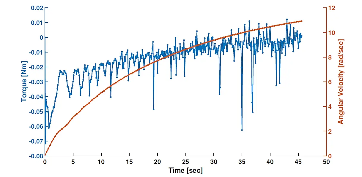
Figure 7 compares the net torque and $$J. \alpha$$ where $$J$$ is the turbine’s mechanical inertia. The agreement between the curves shows that, as expected, the torque values obtained from experiments (Equation (3)) and computations (Equation $$\left(2\right)$$) agree, which provides a consistency check on the numerical method.
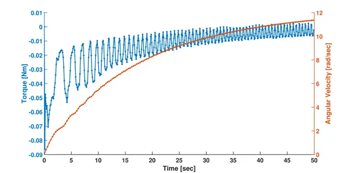
Figure 6. Time histories of net hydrodynamic torque and turbine angular velocity for Case C1. The decreasing amplitude of torque oscillations indicates convergence toward steady-state operation.
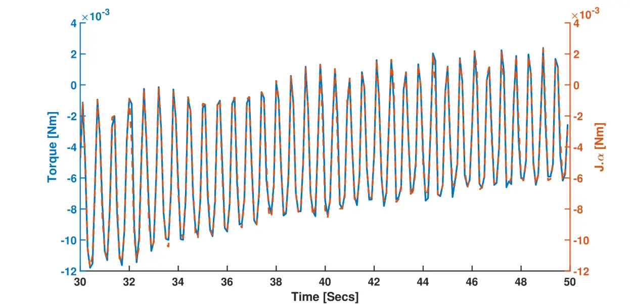
Figure 7. Comparison of the experimentally derived torque $$J·\alpha$$ and the computed hydrodynamic torque for Case C1, demonstrating consistency between the experimental measurements and the numerical model.
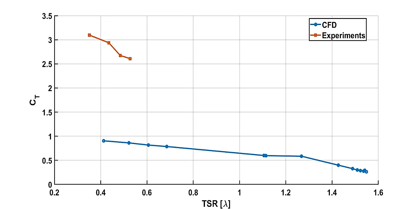
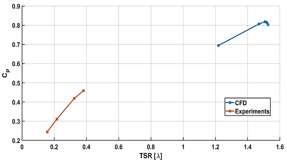
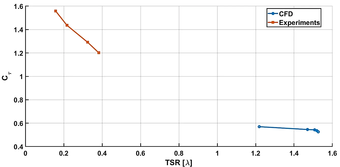
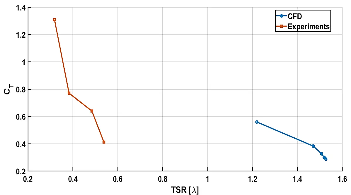
The plots of $${C}_{P}$$ and $${C}_{\tau }$$ versus $$\lambda$$ for Case C1 are shown in Figure 8, and the plots of $${C}_{P}$$ and $${C}_{T}$$ versus $$\lambda$$ are presented in Figure 9. Figure 10, Figure 11 and Figure 12 compare the experimental $${C}_{P}$$, $${C}_{\tau }$$, and $${C}_{T}$$ from [2] with the CFD results for a three-flight turbine inclined at β = 30° in the first configuration.
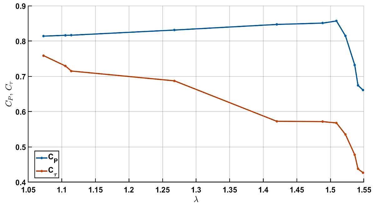
Figure 8. Computed power coefficient $${C}_{P}$$ and torque coefficient $${C}_{\tau }$$ as functions of tip speed ratio $$\lambda$$for case C1. Each point corresponds to an individual CFD simulation.
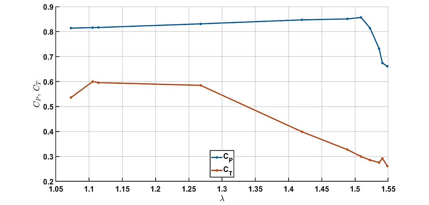
Figure 9. Computed power coefficient $${C}_{P}$$ and thrust coefficient $${C}_{T}$$ as functions of tip speed ratio $$\lambda$$ for Case C1.
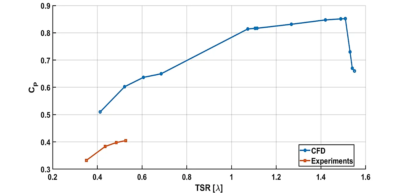
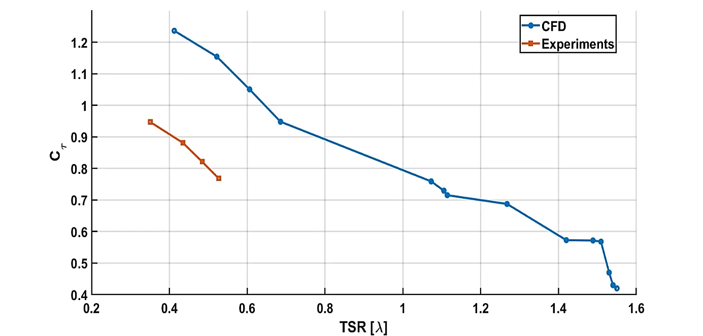
Although the CFD simulations tend to overpredict the turbine performance coefficients relative to experimental measurements, several key features of the turbine behaviour are reproduced consistently. In particular, the simulations capture periodic torque fluctuations as did the experiments and predict the correct order of magnitude of the torque ripple. The overall shapes of the performance curves as functions of tip speed ratio are also similar between the simulations and the measurements. These agreements provide confidence that the numerical model captures the dominant physical mechanisms governing the turbine–flow interaction.
The remaining quantitative differences between the CFD predictions and the experiments are most likely associated with physical effects that were not included in the present simulations. In the experiments, the turbine operated beneath a deformable free surface, whereas the numerical model approximated the upper boundary as a zero-shear surface to reduce computational cost. Free-surface motion can alter the pressure distribution around the turbine, thereby influencing the measured thrust and power coefficients. Moreover, the interaction of the turbine and free surface is likely to be periodic, so the presence of the surface is likely to increase the torque fluctuations. The present simulations, therefore, aim primarily to identify the mechanisms responsible for torque generation, particularly the relative contributions of pressure and viscous forces, rather than to reproduce the experimental performance values exactly.
In Figure 12, the thrust measured in the experiments is significantly higher than the CFD-predicted value. This is also likely attributable to free-surface effects. Moreover, the influence of the free surface on the shaft connecting the turbine to the instrumentation in the experiments, an effect absent in the CFD setup, may reduce power output while increasing thrust. These factors may contribute to the differences observed in $${C}_{P}$$ between experiment and CFD.
Overall, Figure 10, Figure 11 and Figure 12 suggest a substantial free-surface influence, which is expected to reduce power output because energy is expended to sustain the free-surface motion. Similar discrepancies between simulations neglecting free-surface effects and laboratory measurements have been reported in other studies of hydrokinetic turbines [13,14].
3.1.1. Velocity Field
Figure 13 shows the contour of instantaneous water velocity magnitude around the turbine at t = 30 s for Case C1. The low-velocity regions immediately upstream and downstream of the turbine indicate stagnation zones near the shaft and blades.
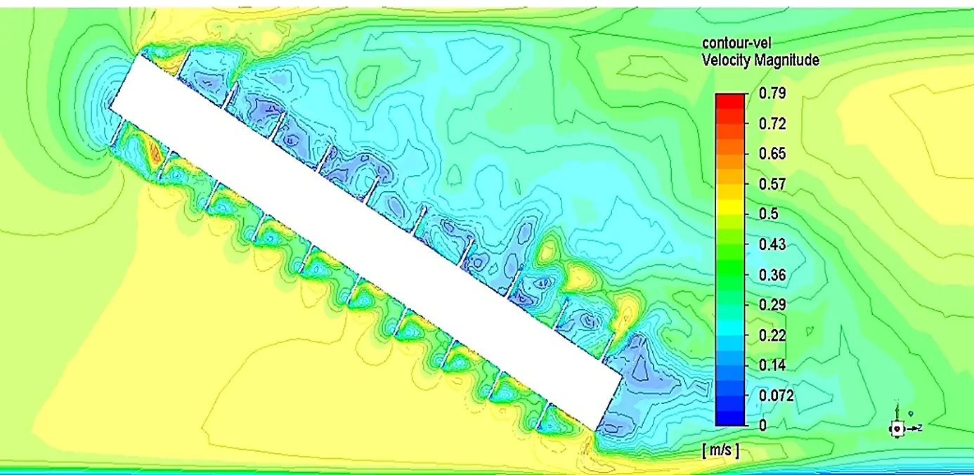
Figure 13. Instantaneous contours of velocity magnitude around the turbine for Case C1 at time t = 30 s. Regions of reduced velocity upstream and downstream of the turbine indicate stagnation zones near the shaft and blades. Flow is from left to right.
Figure 14 provides a close-up view of the velocity vectors around the blades and highlights flow stagnation on the downstream side of the shaft and blades. The results show no significant flow separation or recirculation regions around the turbine, in agreement with the PIV-derived streamlines reported in [2]. It also shows that most of the velocity deficit relative to the freestream occurs within the blade passages, a region not accessible in the PIV measurements of [3].
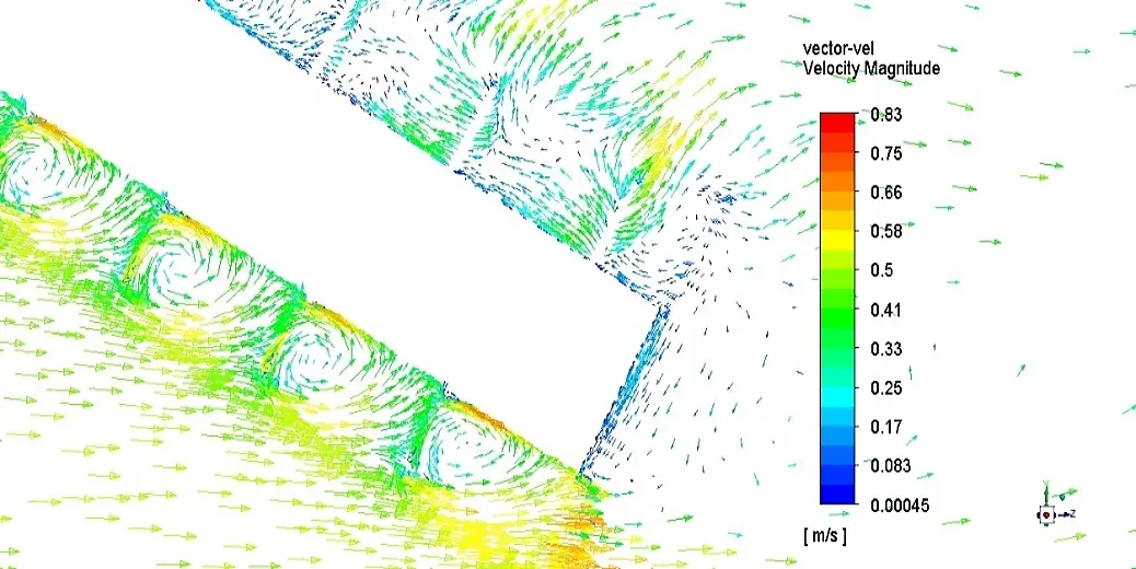
Figure 14. Close-up view of velocity vectors around the turbine blades for Case C1 t = 30 s, illustrating flow behaviour within the blade passages and the absence of significant flow separation. Flow is from left to right.
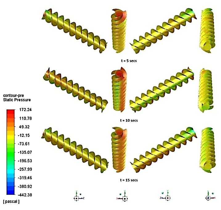
3.1.2. Pressure Field
The blade-surface pressure field for Case C1 is presented in Figure 15. The pressure is notably higher on the top and underside of the turbine in this configuration. A cross-section through the turbine showing the pressure distribution (Figure 16) confirms that the highest pressures occur on these surfaces. The figure also shows that, on the underside of the turbine, the pressure on the front (flow-facing) blade surfaces is greater than that on the back (downstream) surfaces, illustrating the mechanism of torque generation. Additionally, the results indicate that the flow within the blade passages behaves largely independently of the external flow and that most pressure variations occur internally. This behaviour is characteristic of reaction turbines, suggesting that the AST may be classified as a reaction turbine. However, unlike most reaction turbines, the AST does not require a high volumetric flow rate and can operate effectively at low flow rates.
 |
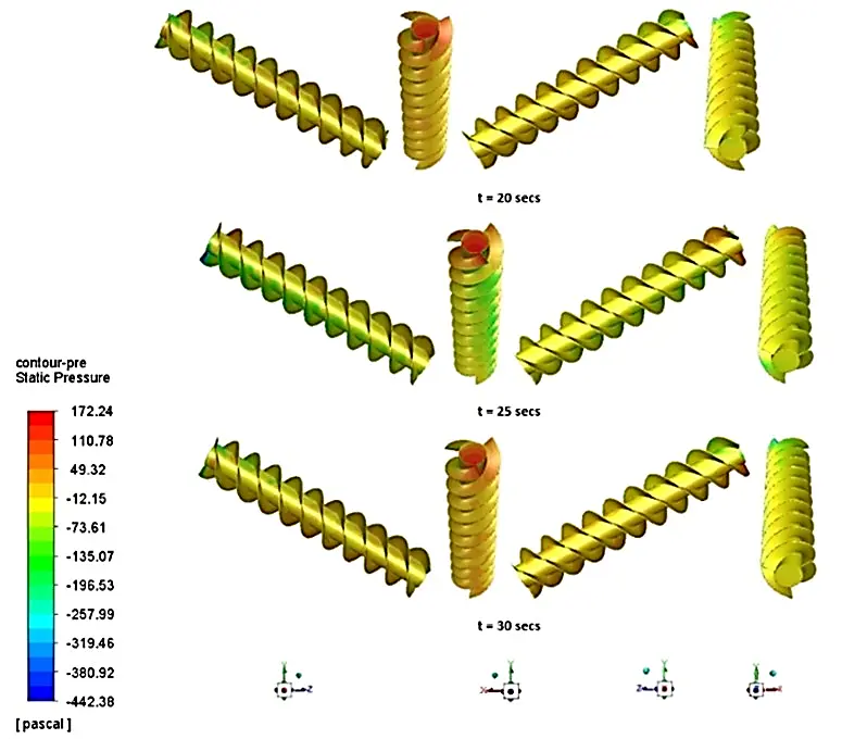 |
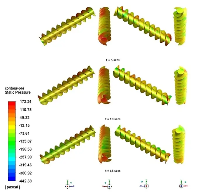
Figure 15. Pressure distribution on the blade surfaces of the three-flight turbine for Case C1. High-pressure regions on the flow-facing surfaces of the blades contribute to the generation of torque.
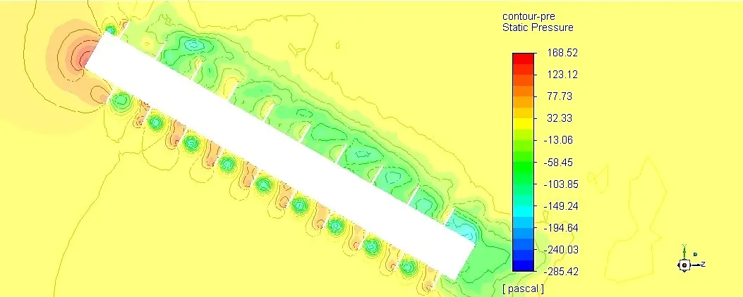
Figure 16. Cross-sectional view of pressure contours around the turbine blades for Case C1, illustrating the pressure difference between the upstream and downstream blade surfaces responsible for torque generation.
Figure 17 shows the pressure difference between the front and back faces of a rotating blade at three axial locations. The pressure difference is sampled at a fixed location on the rotating blade surface. The turbine completes one revolution in approximately 0.55 s, and the pressure signal exhibits a corresponding periodic component. The largest pressure difference occurs at the top of the blade, closest to the free surface.
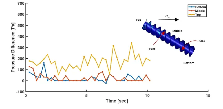
Figure 17. Temporal variation of pressure difference between the front and back faces of a blade at three axial locations for Case C1. The periodic variation corresponds to the rotational motion of the turbine.
As can be seen by the large difference in the vertical scales, Figure 18 and Figure 19 show the torque generation is dominated by pressure forces, while viscous contributions act to reduce the net torque and remain comparatively small. This behaviour occurs at the relatively low Reynolds numbers of the present experiments and simulations ($$Re \approx 4.5×{10}^{4}$$) implies that Reynolds-number effects, which are primarily associated with viscous forces, are minor, and that strong dynamic similarity exists for geometrically similar ASTs across a wide range of sizes, provided the turbine is not extremely small. The Reynolds number is defined using the turbine outside diameter $$D$$ and free-stream velocity $${U}_{\mathrm{\infty }}$$, $$Re={U}_{\mathrm{\infty }}D/\nu$$.
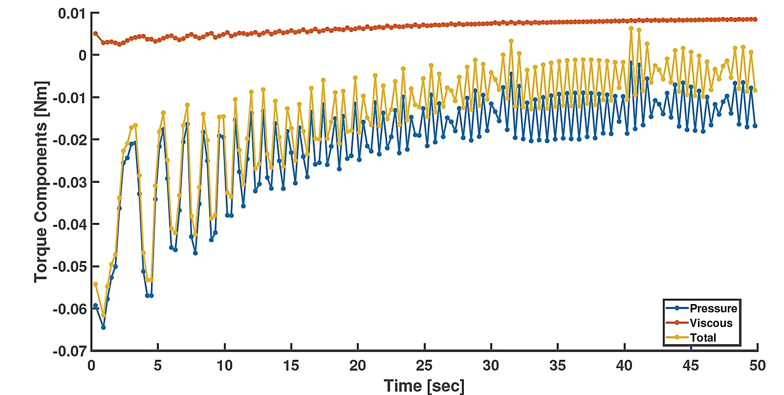
Figure 18. Contributions of pressure and viscous forces to the torque about the turbine axis for Case C1. Pressure forces dominate the torque generation while viscous effects act to slightly reduce the net torque.
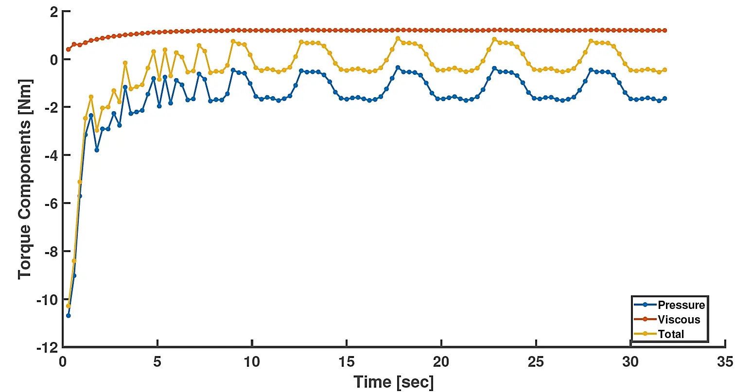
Figure 19. Contributions of pressure and viscous forces to the turbine torque for Case C3 at higher free-stream velocity, showing the continued dominance of pressure forces.
3.2. Second Configuration
Figure 20 presents the torque and angular velocity versus time for the second configuration. As in the first configuration, the torque exhibits periodic variation with angular position.
Plots of $${C}_{P}$$ and $${C}_{\tau }$$ against $$\lambda$$ for Case C2 are provided in Figure 21, while Figure 22 shows $${C}_{P}$$ and $${C}_{T}$$ against $$\lambda$$. Figure 23, Figure 24 and Figure 25 compare the experimental and CFD predictions of $${C}_{P}$$, $${C}_{\tau }$$ and $${C}_{T}$$ over the same range of $$\lambda$$.
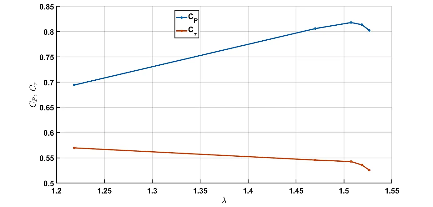
Figure 21. Computed power coefficient $${C}_{P}$$ and torque coefficient $${C}_{\tau }$$ as functions of tip speed ratio $$\lambda$$for case C2. Each point corresponds to an individual CFD simulation.
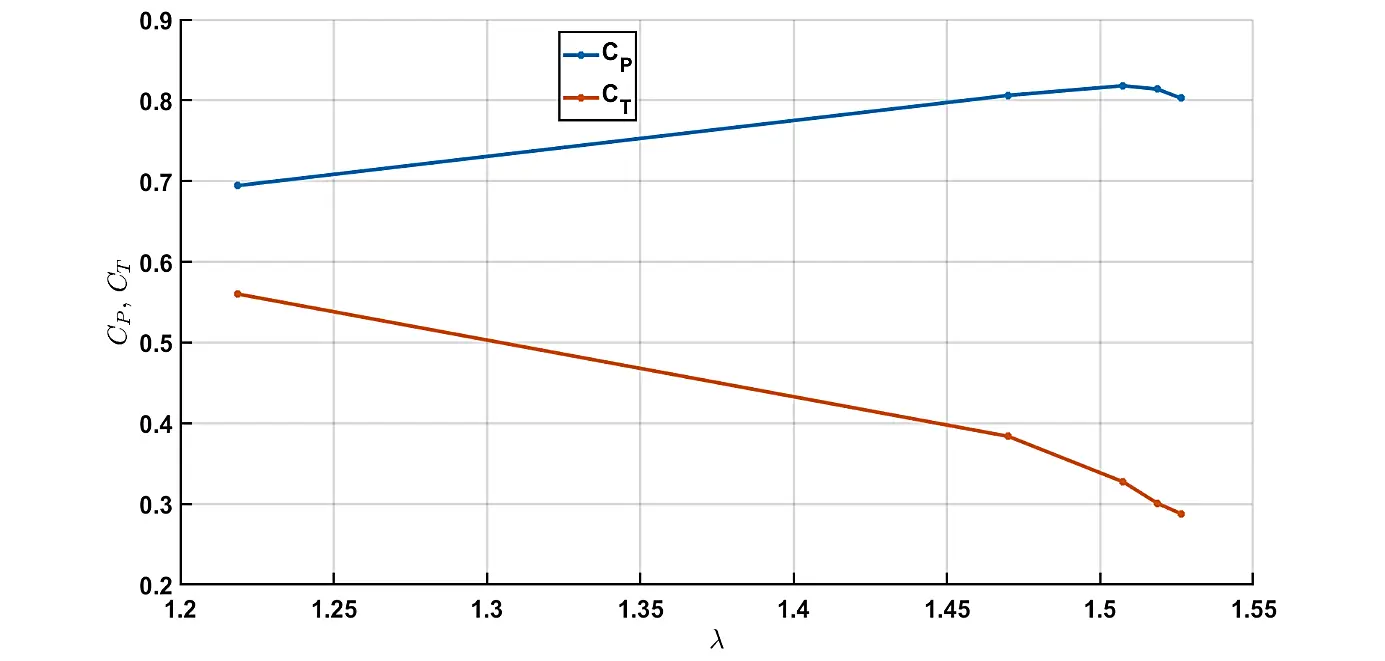
Figure 22. Computed power coefficient $${C}_{P}$$ and thrust coefficient $${C}_{T}$$ as functions of tip speed ratio $$\lambda$$ for Case C2.
3.2.1. Velocity Field
Figure 26 shows the velocity contours for Case C2 at a flow time of t = 37 s, and Figure 27 displays a close-up view of the corresponding velocity vectors.
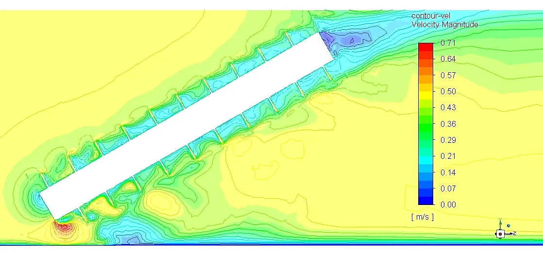
Figure 26. Instantaneous contours of velocity magnitude around the turbine for Case C2 at time t = 37 s. Flow is from left to right.
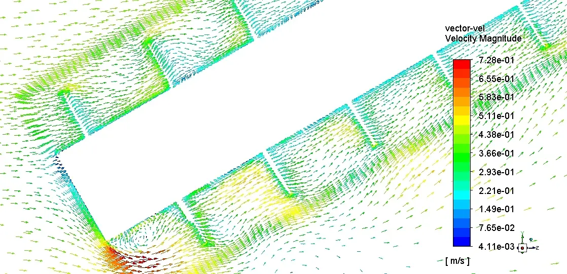
Figure 27. Close-up view of velocity vectors around the turbine blades for Case C2 t = 37 s, illustrating flow behaviour within the blade passages and the absence of significant flow separation. Flow is from left to right.
3.2.2. Pressure Field
Figure 28 shows the pressure distribution on the turbine blades for Case C2. In this configuration, the highest pressures occur in the bottom and top regions of the turbine. A cross-section of the blades (Figure 29) confirms this pattern. Figure 30 shows the temporal variation of the pressure difference between the front (flow-facing) and back (downstream) faces of a single blade. Here, the greatest pressure difference occurs at the bottom of the blade. As with the first configuration, the pressure difference is sampled at a fixed location on the rotating blade surface. The turbine completes one revolution in approximately 0.57 s.
 |
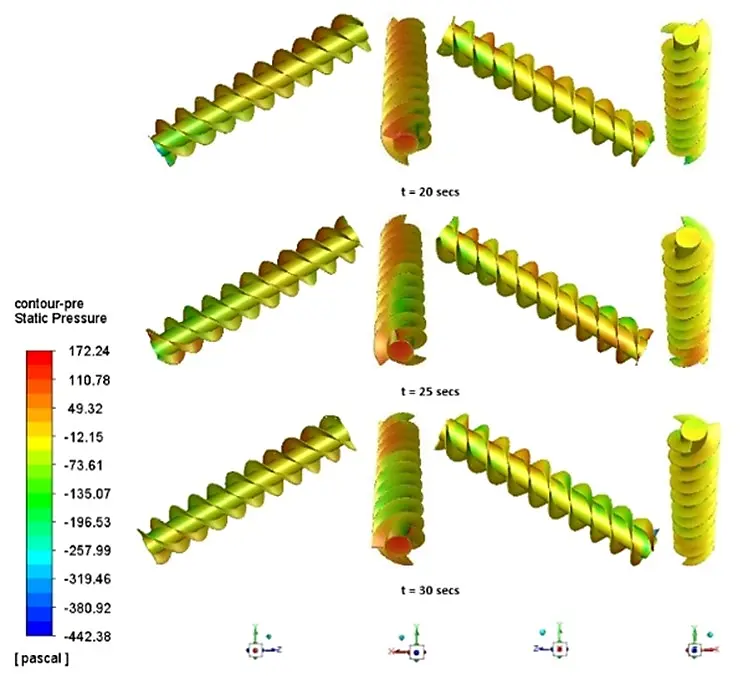 |
Figure 28. Pressure distribution on the blade surfaces of the three-flight turbine for Case C2. High-pressure regions on the flow-facing surfaces of the blades contribute to the generation of torque.
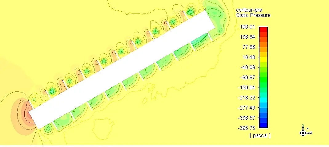
Figure 29. Cross-sectional view of pressure contours around the turbine blades for Case C2, illustrating the pressure difference between the upstream and downstream blade surfaces responsible for torque generation.
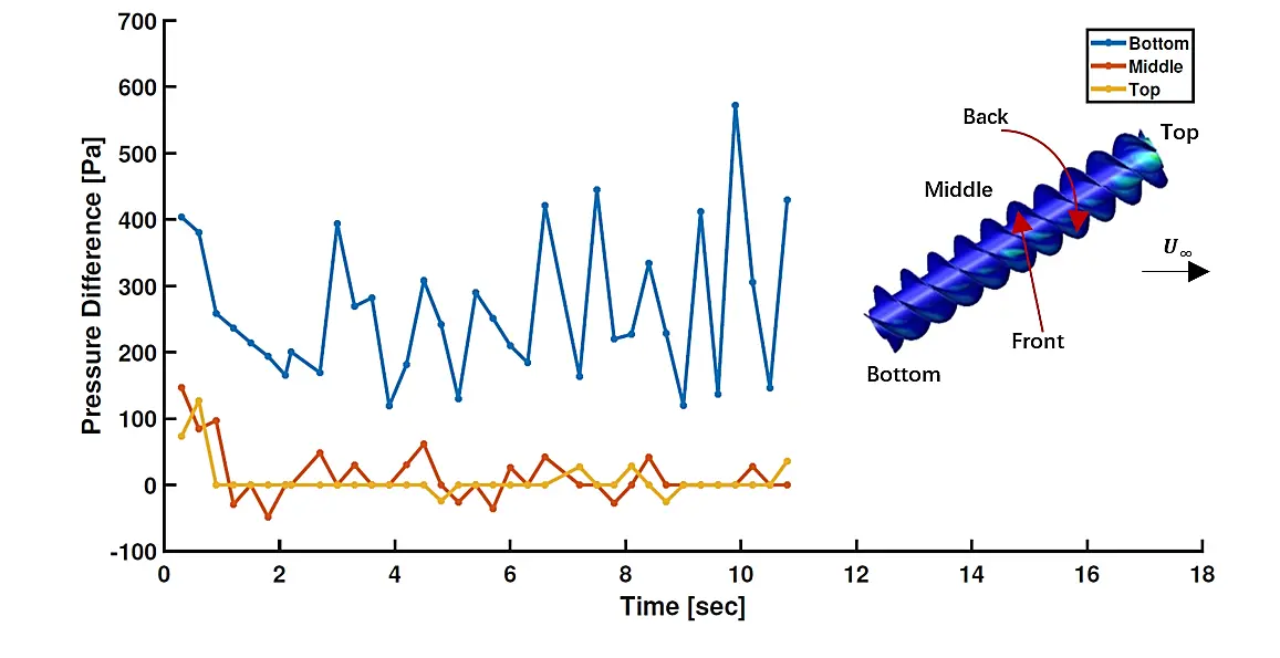
Figure 30. Temporal variation of pressure difference between the front and back faces of a blade at three axial locations for Case C2. The periodic variation corresponds to the rotational motion of the turbine.
3.3. Cavitation
The potential for cavitation was assessed using the pressure fields from Cases C1 and C3. Cavitation is described by the dimensionless cavitation factor, $$\sigma$$:
|
```latex\sigma =\mathrm{ }\frac{{P}_{\mathrm{\infty }}-\mathrm{ }{P}_{v}}{\frac{1}{2}\rho {U}_{\mathrm{\infty }}^{2}}``` |
(9) |
where $${P}_{\mathrm{\infty }}$$ is the reference water vapour pressure (free stream pressure), and $${P}_{v}$$ is the saturated water vapour pressure. Cavitation is examined by comparing $$\sigma$$ with the local pressure coefficient, $${P}_{P}$$, which characterizes hydrodynamic loading, and depends on the blade geometry and Reynolds number [15,16].
|
```latex{P}_{P}=\mathrm{ }\frac{P-\mathrm{ }{P}_{\infty }}{\frac{1}{2}\rho {U}_{\mathrm{\infty }}^{2}}``` |
(10) |
where $$P$$ is the local pressure on the blade surface. Cavitation will occur when $${P}_{P} < -\sigma .$$ Thus, the condition $$\sigma + {P}_{P} \ge 0$$ must hold near the blade surfaces to avoid cavitation.
The cavitation factor computed from Equation $$\left(9\right)$$ was compared with the local pressure coefficient from Equation $$\left(10\right)$$, as shown in Figure 31 and Figure 32, indicating a tendency toward cavitation at high free-stream velocities.
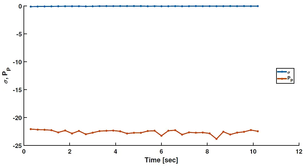
Figure 31. Time variation of cavitation factor $$\sigma$$ and pressure coefficient $${P}_{P}$$ for Case C1. The results indicate that cavitation is unlikely under experimental operating conditions.
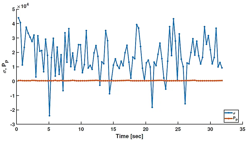
Figure 32. Comparison of cavitation factor $$\sigma$$ and pressure coefficient $${P}_{P}\mathrm{ }$$ against time for Case C3. The results suggest a tendency toward cavitation at higher free-stream velocities.
4. Discussion and Conclusions
CFD simulations were performed using the SST $$k-\omega \bm{ }$$ turbulence model for a turbine with three flights in both configurations. This turbine gave the maximum measured power coefficients in the experiments in [2]. Flow-induced simulations were employed to reproduce the torque ripples observed experimentally accurately. These ripples necessitated time-dependent calculations to ensure that the turbulence model could respond to cyclic torque variations. The PIV experiments showed no strong periodicity or large recirculation regions in the flow field outside the blades, supporting the use of a URANS approach. The simulations also indicated no significant cyclic variations in the external flow. It was assumed, therefore, that turbulent processes occurred on timescales smaller than the turbine’s rotational period. Flow-induced simulations were also chosen to replicate the experimental procedure described in [2], where torque and angular acceleration were measured on a freely rotating turbine subjected to flow-induced loading.
A key insight emerging from the CFD simulations is not simply that torque generation is dominated by pressure forces, but that this behaviour already occurs at the relatively low Reynolds numbers of the present experiments and simulations. The decomposition of the torque into pressure and viscous components shows that viscous effects contribute only a small fraction of the total torque and primarily act to reduce the net torque. The Reynolds number of the present study, based on the turbine outside diameter and free-stream velocity, is approximately $$Re\approx 4.5×{10}^{4}$$. By comparison, the full-scale Cat 3EC42 turbine reported by Shahsavarifard et al. [4] operates at Reynolds numbers of order $${10}^{6}$$ (two orders of magnitude larger than the present study). The present results therefore indicate that the Archimedes screw turbine behaves primarily as a pressure-driven reaction turbine even in a relatively low-Reynolds-number regime. This suggests that Reynolds-number dependence becomes weak at Reynolds numbers lower than those likely to be encountered in practice, implying strong dynamic similarity for geometrically similar ASTs across much of their operating range. This result helps explain why laboratory-scale experiments can provide useful insight into the performance of full-scale AST devices.
The simulations also reveal that the flow behaviour within the blade passages is largely decoupled from the external flow field surrounding the turbine. This finding helps explain the absence of strong cyclic variations in the PIV measurements reported in [3], despite significant torque oscillations observed experimentally. Since optical measurements cannot access the flow inside the blade passages, CFD provides valuable insight into the internal pressure distributions responsible for the turbine loading.
These results provide new understanding of the physical mechanisms governing energy extraction in the AST and suggest that geometric parameters affecting blade pressure distribution may play a more significant role in determining turbine performance than viscous scaling effects.
The agreement between the simulated torque ripple behaviour and the experimental observations further supports the ability of the numerical model to capture the dominant turbine–flow interaction mechanisms.
In the first configuration, the turbine performed better in CFD than in the experiments, achieving a maximum $${C}_{P}$$ of 0.85 at $$\lambda$$ = 1.50, compared to an experimental maximum of 0.40 at $$\lambda$$ = 0.53 [2]. In contrast to the experiments, the two configurations performed similarly in CFD: the second configuration achieved a $${C}_{P}$$ of 0.82 at $$\lambda$$ = 1.51 (experiment: 0.34 at λ = 0.54 [2]). The most likely cause of these discrepancies is the absence of free-surface modelling in the CFD simulations. Free-surface effects can strongly influence turbine performance and may lead to over-predictions in CFD when neglected. The consistent overprediction of performance metrics across both configurations compared to the experimental results strongly suggests that free-surface effects, rather than numerical artefacts, are the dominant source of discrepancy.
Pressure data from simulations at free-stream velocities of 0.45 m/s and 6.75 m/s were used to assess the potential for cavitation. A comparison of the cavitation factor and the local pressure coefficient indicates a likelihood of cavitation at high free-stream velocities.
Although the present simulations provide useful insight into the mechanisms governing torque generation in the Archimedes screw turbine, several modelling simplifications were necessary. In particular, free-surface motion was not explicitly simulated, and the upper boundary was approximated as a zero-shear surface in order to maintain tractable computational cost. Future CFD studies incorporating a deformable free surface may provide improved quantitative agreement with experimental measurements and further clarify the influence of surface effects on turbine performance.
5. Recommendations and Future Work
There remain numerous, and genuinely compelling, opportunities for future research on the AST. Significant aspects of the turbine’s behaviour are still not fully understood, and it likely conceals further insight within its seemingly simple helical geometry. Any analysis that enhances our understanding of the flow mechanisms governing power extraction would be especially valuable. Several directions for subsequent studies are outlined below. Pursuing these lines of inquiry would advance our knowledge of the turbine and accelerate its development into a reliable and efficient producer of renewable energy in suitable resource environments.
CFD can be employed to investigate the influence of surface effects on the performance of the two turbine configurations examined in this work. Such studies may clarify whether configuration-specific differences remain negligible when surface effects are minimal or become more pronounced under particular conditions.
Blockage effects and their associated corrections were not incorporated in the present study due to the limitations discussed in Section 2. Given the relatively high blockage ratio encountered in [2,3] (and which was replicated in the simulations in this paper), targeted investigations into blockage-related performance changes are essential. Understanding the magnitude and nature of blockage effects is critical for interpreting past results and for designing future experiments or deployment scenarios.
Torque ripple represents another phenomenon requiring deeper investigation. Its origins and impacts are still not well understood, yet it may have important implications for turbine efficiency and for the durability of components such as the drivetrain and generator. Cyclic variations in torque have been observed in both experimental measurements and in blade pressure distributions obtained from CFD. However, no definitive causal mechanism has been identified, nor has a clear relationship with the surrounding flow field been established. Notably, PIV results do not indicate large cyclic perturbations outside the blades that would correspond to the detected torque fluctuations.
CFD results indicate that torque generation in the AST is predominantly pressure-driven. A key question for future research is how blade geometry, including blade shape and the number of flights, modulates this behaviour. Determining whether blade shape meaningfully affects performance, as is typical for many other turbine types, or whether its influence is minimal in the AST’s case, would significantly inform design optimization.
Statement of the Use of Generative AI and AI-Assisted Technologies in the Writing Process
During the preparation of this manuscript, the author(s) used Grammarly in order to check spelling, grammar, punctuation, and typographical errors within the manuscript. After using this tool/service, the author(s) reviewed and edited the content as needed and take(s) full responsibility for the content of the published article.
Acknowledgments
The authors are grateful to the Schulich endowment to the University of Calgary for financial support. The authors would also like to thank Chris Morton, Ayman Ashry Mohammed, and Itoje Harrison for technical support with this project.
Author Contributions
Conceptualization, T.E.P. and D.H.W.; Methodology, T.E.P. and D.H.W.; Writing—Original Draft Preparation, T.E.P.; Writing—Review and Editing, D.H.W.; Supervision, D.H.W.
Ethics Statement
Not applicable.
Informed Consent Statement
Not applicable.
Data Availability Statement
Data is available on request.
Funding
This project was supported by the Schulich endowment to the University of Calgary.
Declaration of Competing Interest
The authors declare that they have no known competing financial interests or personal relationships that could have appeared to influence the work reported in this paper.
References
-
Williamson S, Stark B, Booker J. Low head pico hydro turbine selection using a multi-criteria analysis. In World Renewable Energy Congress; Moshfegh PB, Ed.; Linköping University Electronic Press: Linköping, Sweden, 2011; pp. 1377–1385. [Google Scholar]
-
Phillips TE, Wood DH. Performance characteristics of the Archimedes screw hydrokinetic turbine. Ocean. Eng. 2025, 339, 122062. DOI:10.1016/j.oceaneng.2025.122062 [Google Scholar]
-
Phillips TE, Wood DH. Study of the Flow Field around the Archimedes Screw Hydrokinetic Turbine using Particle Image Velocimetry. Ocean. Eng. 2025, Submitted. [Google Scholar]
-
Shahsavarifard M, Birjandi AH, Bibeau EL, Sinclaire R. Performance Characteristics of the Energy Cat 3EC42 Hydrokinetic Turbine. In Proceedings of the MTS/IEEE OCEANS 2015—Genova: Discovering Sustainable Ocean Energy for a New World, Genova, Italy, 18–21 May 2015; pp. 1–4. DOI:10.1109/OCEANS-Genova.2015.7271420 [Google Scholar]
-
Zitti G, Fattore F, Brunori A, Brunori B, Brocchini M. Efficiency evaluation of a ductless Archimedes turbine: Laboratory experiments and numerical simulations. Renew. Energy 2020, 146, 867–879. DOI:10.1016/j.renene.2019.06.174 [Google Scholar]
-
ANSYS. ANSYS Fluent User’s Guide; ANSYS Inc.: Canonsburg, PA, USA, 2013. [Google Scholar]
-
ANSYS. ANSYS Fluent Theory Guide; 2021 R2; ANSYS Inc.: Canonsburg, PA, USA, 2021. [Google Scholar]
-
Menter FR. Zonal Two Equation k-ω Turbulence Models for Aerodynamic Flows. In AIAA 24th Fluid Dynamics Conference; American Institute of Aeronautics and Astronautics: Orlando, FL, USA, 1993; pp. 1–21. [Google Scholar]
-
Menter FR. Two-Equation Eddy-Viscosity Turbulence Models for Engineering Applications. AIAA J. 1994, 32, 1598–1605. DOI:10.2514/3.12149 [Google Scholar]
-
Simmons SC, Lubitz WD. Analysis of internal fluid motion in an Archimedes screw using computational fluid mechanics. J. Hydraul. Res. 2021, 59, 932–946. DOI:10.1080/00221686.2020.1844813 [Google Scholar]
-
Adhikari RC, Vaz J, Wood D. Cavitation inception in crossflow hydro turbines. Energies 2016, 9, 237. DOI:10.3390/en9040237 [Google Scholar]
-
Ribau ÂM, Gonçalves ND, Ferrás LL, Afonso AM. Flow structures identification through proper orthogonal decomposition: The flow around two distinct cylinders. Fluids 2021, 6, 384. DOI:10.3390/fluids6110384 [Google Scholar]
-
Benavides-Morán A, Rodríguez-Jaime L, Laín S. Numerical Investigation of the Performance, Hydrodynamics, and Free-Surface Effects in Unsteady Flow of a Horizontal Axis Hydrokinetic Turbine. Processes 2021, 10, 69. DOI:10.3390/pr10010069 [Google Scholar]
-
Benchikh Le Hocine AE, Jay Lacey RW, Poncet S. Multiphase modeling of the free surface flow through a Darrieus horizontal axis shallow-water turbine. Renew. Energy 2019, 143, 1890–1901. DOI:10.1016/j.renene.2019.06.010 [Google Scholar]
-
Adhikari R. Design Improvement of Crossflow Hydro Turbine. Ph.D. Thesis, University of Calgary, Calgary, AB, Canada, 2016. DOI:10.11575/PRISM/25581 [Google Scholar]
-
Silva PA, Shinomiya LD, de Oliveira TF, Vaz JR, Mesquita AL, Junior AC. Analysis of cavitation for the optimized design of hydrokinetic turbines using BEM. Appl. Energy 2017, 185, 1281–1291. DOI:10.1016/j.apenergy.2016.02.098 [Google Scholar]