Collaborative Optimization of Berth Allocation and Marine Energy Utilization for Low-Carbon Ports

Renewable Energy (MRE), mainly including offshore wind power and offshore photovoltaic, is a clean and renewable energy source with broad development prospects. Ports are important nearshore terminals for MRE consumption and conversion [1]. The heavy reliance of traditional seaports on fossil fuels has resulted in severe air pollution and substantial carbon emissions [2]. In 2023, the International Maritime Organization set an emission reduction milestone, targeting a 20% reduction in total greenhouse gas emissions by 2030 compared to the 2008 level [3]. Propelled by the dual impetus of the dual carbon goals and global supply chain restructuring, ports are now confronting the dual challenges of enhancing operational efficiency and promoting low-carbon transformation [4]. Among these challenges, improving berth utilization efficiency and optimizing the energy supply structure have become key issues for the sustainable development of ports [5,6]. The MRE takes the ocean as the spatial carrier and has the characteristics of cleanness and renewability; offshore natural gas, as a low-carbon fossil energy, is an important transitional energy for the low-carbon transformation of ports due to its lower carbon emission intensity. Existing reviews have summarized port energy efficiency technologies, operational strategies, and energy management systems, but most studies focus on independent optimization of a single system, lacking collaborative optimization of berth allocation, flexible load regulation, and low-carbon energy supply [7]. The study fills this gap by integrating MRE utilization into the joint optimization of port logistics and energy systems.

Traditional ports rely heavily on fossil fuels and onshore power grids, leading to high carbon emissions and low efficiency of marine energy utilization. Therefore, integrating offshore renewable energy sources (offshore wind power, offshore photovoltaic) and low-carbon fossil energy (offshore natural gas) into the coordinated optimization of berth allocation and energy management [8]. Recent studies on port energy systems have begun to focus on marine energy integration. For example, Parhamfar et al. [9] proposed a port microgrid scheduling model incorporating offshore wind power but failed to coordinate with berth allocation. Integrating marine energy sources (offshore wind power, photovoltaic, and natural gas) into the coordinated optimization of berth allocation and energy management can effectively reduce carbon emissions and build green ports.

The key to building a green port lies in the coordinated optimization of logistics and energy scheduling systems. The port’s logistics-energy scheduling system mainly consists of three parts: ships, shores, and port areas. The berth allocation problem (BAP) involving interactions between ships and shores constitutes the core task of logistics scheduling. Early BAP research focused on solving methods such as mixed-integer linear programming [10] and genetic algorithms [11]. Aslam et al. [12] verified the applicability of the cuckoo search algorithm (CSA) in multi-berth allocation problems, whose strong global search capability shows significant advantages over other intelligent algorithms in both solving speed and solution quality. Recent research trends have shifted toward the joint scheduling of the BAP with other onshore resources, covering the coordinated optimization of BAP and quay cranes (QC) [13], BAP and shore power [14], as well as BAP and container logistics scheduling [15]. These above mentioned links form a cascaded scheduling of the logistics system, enabling the optimization of port resource scheduling to move from independent optimization to overall optimization. In addition, the optimization objectives of BAP have shifted from single-objective static planning to multi-objective dynamic optimization [16]. Ma et al. [17] constructed a two-stage distributionally robust optimization model for the port integrated energy system under dual uncertainties of wind power output and ship arrival time. Pu et al. [18] combine the column-and-constraint generation algorithm with the adaptive alternating direction method of multipliers, thereby achieving distributed coordination and robust optimal scheduling of the energy-logistics system. Despite the significant progress made in BAP in terms of solving efficiency and coordinated optimization with port equipment, existing studies mostly proceed from the single perspective of port operations, lacking detailed modeling of berthing costs between ships and port operators. This perspective limitation fails to fully stimulate the subjective initiative of arriving ships to independently participate in shore power usage and dynamic adjustments of berth allocation.

The energy consumption behavior of onshore electrified equipment in logistics links determines the load distribution characteristics of port energy systems. Optimizing the energy system involving interactions between shores and port areas is the core issue of energy scheduling, focusing on two key domains: supply-side power management and demand-side load response. In terms of supply-side power management, the multi-energy complementarity of distributed energy sources (DES) and renewable energy units, along with their low-carbon and economic performance, has become a research hotspot [19]. Li et al. [20] innovatively introduced a heterogeneous energy sharing mechanism into the field of regional energy coordinated optimization. Ma et al. [21] enhanced the stability and resilience of port power management through a coordinated configuration framework of soft open points (SOP) and energy storage systems (ESS) in port integrated energy systems. Tang et al. [22] designed a multi-time scale scheduling strategy based on hydrogen-electricity coupling to optimize the operation of hydrogen-electricity coupled systems and improve renewable energy utilization efficiency. Wang et al. [23] incorporated the charging-discharging characteristics of electric vehicles into multi-energy complementary systems, achieving synergistic complementarity with the power grid. These studies provide insights for fully leveraging the charging-discharging and energy storage characteristics of electric trucks on the energy supply side.

In terms of demand-side load response, its core role lies in exploring and utilizing flexible loads, enhancing load controllability to optimize load curves, mitigate load fluctuations, and thereby improve system safety and economy [24]. Astriani et al. [25] realized microgrid demand response by shifting specific loads from peak periods to off-peak periods to reduce load consumption. Zhang et al. [26] proposed a price-response-based load elasticity matrix and a compensation pricing mechanism for response participation, optimizing the total system cost through reasonable compensation for users participating in load response. Wang et al. [27] construct a decentralized demand response (DR) market based on peer-to-peer transactions. This market mechanism endows customers with a certain degree of pricing power, enhancing their bargaining capacity when interacting with multiple buyers in a competitive environment. However, port energy-consuming equipment mainly includes quay cranes, yard cranes, trucks, and shore power, while cold-consuming equipment primarily comprises refrigerated containers and cold storage. The volatility, correlation, and spatiotemporal distribution characteristics of their electric and cold loads differ significantly from those of traditional park energy systems. Therefore, it is necessary to construct a demand response mechanism that balances rationality and adaptability for shore-side equipment. The above content has detailed the current research on port logistics scheduling and energy optimization, respectively. The concept of their joint scheduling optimization was first proposed in 2022. Zhang et al. [28] designed a two-stage model for optimal day-ahead scheduling, and the proposed joint scheduling algorithm effectively improved the overall system efficiency, operational reliability, and economy of the port microgrid. Mao et al. [29] constructed a basic ship-port collaborative energy model covering onshore power supply management and berth allocation and proposed an integrated energy system scheduling model. Subsequently, Li et al. [30] proposed a robust optimization strategy based on the info-gap decision theory for the three-dimensional coordinated scheduling of port berths, logistics, and multi-energy systems. Although the studies all focus on the coordinated optimization of the port logistics-energy scheduling system, their emphasis is more on the field of logistics scheduling. In terms of energy optimization, they only remain at the level of simple multi-energy complementarity and fail to fully consider low-carbon goals. Recently, Zhou et al. [31] proposed a two-layer energy scheduling model based on the Stackelberg game: the microgrid operator as leader formulates energy pricing and optimizes resource allocation, while the ship operating company as follower adjusts flexible load demands. Shi et al. [32] propose a two-level Nash-Stackelberg-Nash game framework, comparing the scheduling results of the seaport integrated energy system and seaport logistics system under cooperative and non-cooperative strategies. Even though the above studies apply game theory to the coordinated optimization of SIES and SLS, their core focus remains on the energy demands of berthed ships. However, shore-side electrified equipment is the largest energy-consuming entity in ports. Therefore, there is an urgent need for detailed analysis and optimization of the energy demands throughout the entire logistics process.

To achieve the collaborative optimization of port berth scheduling, energy transition, and load response, this study proposes a two-stage progressive optimization framework based on the improved CSA and Stackelberg game theory. In the first stage, the improved CSA is applied to solve the berth allocation problem, obtain berth allocation results, and load curves of port equipment (including real-time power consumption of quay cranes, yard cranes, electric trucks, shore power, and cooling load of refrigerated containers). These curves reflect the time-varying energy demand driven by berth scheduling and serve as key input parameters for the second-stage energy system optimization. Subsequently, these load curves are used as basic input parameters for the Stackelberg game in the second stage, where dynamic optimization is performed on the energy transaction prices of port energy operators (PEO), the load demand responses of port equipment aggregators (PEA), and the unit output of distributed energy suppliers (DES). Meanwhile, to fulfill the goal of building a low-carbon port, a carbon emission penalty mechanism is established targeting the two major carbon emission sources, namely ship auxiliary engines and distributed energy generation units. The core contributions of this study are as follows:

The collaborative optimization model for berth allocation and power management within port energy systems is illustrated in Figure 1. The carbon emission cost is integrated with the TOU electricity pricing mechanism to generate an optimal berth allocation scheme for incoming ships in the first stage. A demand response load matrix model and a tripartite energy price game model for the port park are constructed in the second stage. The specific model construction is described as follows.

This section serves as a fundamental component of the progressive two-stage optimization model, establishing a multi-objective optimization model and its constraint model for the berth allocation problem.

Given the port berth layout and the set of ships to be served within the next 24 h, the objective function of the BAP is to minimize the total cost incurred from the service start time to the service end time for all ships:

where $${C_{{\rm{B,total}}}}$$ denotes the sum of the total service costs for all ships; $${C_{{\rm{wait}}}}$$ denotes the sum of the total waiting costs for all ships before berthing; $${C_{{\rm{process}}}}\,$$denotes the sum of the total berthing costs for all ships during berthing.

The total waiting cost of ships comprises three components incurred during the waiting period:

where $${C_{{\rm{wait}},s}}$$ and $$C_{{\rm{fuel,wait}}}^s$$ denote the waiting service cost and the comprehensive cost related to auxiliary engine fuel consumption for sth ship, respectively; $$B{T_s}$$ and $$A{T_s}$$ represent the berthing time and arrival time at the port of ships, respectively; $${\eta _w}$$ is the waiting cost coefficient for sth ship; $${P_s}$$ denotes the auxiliary engine power of sth ship; $${c_{{\rm{fuel}}}}$$, $${\eta _{{\rm{fuel,c}}{{\rm{o}}_2}}}$$ and $${\lambda _{{\rm{c}}{{\rm{o}}_2}}}$$ are the unit cost of marine high-sulfur fuel oil, carbon emission factor, and carbon penalty cost coefficient, respectively, with values set as 0.95 yuan/kW, 0.786 kg/kW, and 0.1 yuan/(kW·h).

When berthed, ships can either connect to shore power or use on-board fuel for power generation, selecting the lower-cost option to meet auxiliary engine power demands. The total berthing cost of ships includes three components incurred during berth:

where $${C_{{\rm{process,}}s}}$$, $${C_{{\rm{optimal}},s}}$$ and $${C_{{\rm{equipment,}}s}}\,$$denote the berthing service cost, optimal power supply cost for auxiliary engines, and energy consumption cost of port equipment for sth ship, respectively; $${\eta _b}$$ represents the unit price of berthing service fees; $$P{T_s}$$ is the berthing duration of sth ship; $${C_{{\rm{shore,}}s}}$$ and $${C_{{\rm{fuel,}}s}}$$ denote the shore power cost and fuel power cost for the auxiliary engine of sth ship, respectively; $${c_{{\rm{e}},t}}$$ is the TOU electricity price at time t; $${P_{{\rm{QC}}}}$$, $${P_{{\rm{YC}}}}$$ and $${P_{{\rm{TR}}}}$$ represent the power of quay cranes (QC), yard cranes (YC), and SBEV, respectively; $$R_{s,{s'}}$$ is the correlation degree between two vessels berthed at adjacent order.

Constraint 1: The actual berth start time of sth ship shall not be earlier than its scheduled arrival time at the port.

Constraint 2: The sum of the berthing start time and the handling time of sth ship shall not exceed its departure time.

where $$H{T_s}$$ and $$D{T_s}$$ denotes the handling time and the departure time of sth ship, respectively.

Constraint 3: For any sth ship, the sum of its berthing start position and its own length shall be less than or equal to the total length of the port berth.

where $$B{P_s}$$ and $${L_s}$$ denotes the berthing start position and the length of sth ship, respectively; $${L_b}$$ stands for the total length of the continuous berth.

Constraint 4: Each ship shall be assigned a unique berthing time and berthing position. This constraint prevents frequent entry or exit of the port caused by multiple allocations.

where: $${x_{sbt}}$$ is a binary variable: it takes a value of 1 if sth ship is assigned to berth position b at time t; otherwise, it is 0; T represents the one-day scheduling cycle, with a value of 24 h.

Constraint 5: For the same berth position and period, only one ship can be served. This constraint ensures that any two ships have no overlap in their berth occupation time and spatial range, preventing berth resource conflicts.

As depicted in Figure 2, serving as the upper tier of the two-stage model, this section centers on constructing models for the objective functions, strategic approaches, and constraint conditions of the three parties involved: PEO, DES, and PEA.

As the core leader in the Stackelberg game within the port energy system, PEO purchases electricity and cool energy from DES and the upper-level energy network, then sells them to PEA to meet demand. By guiding the dynamic adaptation of energy supply and demand through price signals, it ultimately achieves the operational objectives of controlling the economic costs and reducing carbon emissions. Its objective function is expressed as follows:

where: $${F_{{\rm{PEO}}}}$$ is PEO’s objective function; $$I_{{\rm{PEO,e}}}^t$$ and $$I_{{\rm{PEO,c}}}^t$$ denote PEO’s electricity and cooling sales revenue to PEA at time t, respectively; $$C_{{\rm{DES,e}}}^t$$ and $$C_{{\rm{DES,c}}}^t$$ represent PEO’s electricity and cooling purchase costs from DES at time t, respectively; $$C_{{\rm{grid,e}}}^t$$ and $$C_{{\rm{grid,c}}}^t$$ are PEO’s electricity and cooling purchase costs from the upper-level grid at time t, respectively; $$C_{{\rm{grid}},{\rm{c}}{{\rm{o}}_2}}^t$$ is the carbon emission cost from the upper-level grid; $$\Delta t$$ is a specific time interval, the value is set to 1 h.

where $$P_{{\rm{PEO,e}}}^t$$ and $$P_{{\rm{PEO,c}}}^t$$ denote the electricity and cooling power sold by PEO to PEA at time t, respectively; $$\lambda _{{\rm{PEA,e}}}^t$$  and $$\lambda _{{\rm{PEA,c}}}^t$$ represent the unit price of electricity and cooling sold by PEO to PEA at time t, respectively.

where $$P_{{\rm{DES,e}}}^t$$ and $$P_{{\rm{DES,c}}}^t$$ denote the electricity and cooling power purchased by PEO from DES at time t, respectively; $$\lambda _{{\rm{DES,e}}}^t$$ and $$\lambda _{{\rm{DES,c}}}^t$$ represent the unit price of electricity and cooling purchased by PEO from DES at time t, respectively.

where $$P_{{\rm{grid,e}}}^t$$ and $$P_{{\rm{grid,c}}}^t$$ denote the electricity and cooling power purchased by PEO from the upper-level grid at time t, respectively; $$\lambda _{{\rm{grid,e}}}^t$$ represents the TOU electricity price at time t; $$\lambda _{{\rm{grid,c}}}^{}$$ is the cooling price of the upper-level cooling grid.

where $$\eta _{{\rm{coal,c}}{{\rm{o}}_2}}$$ denotes the coal-fired carbon emission factor, the value is set to 1.126 kg/kW.

As the game leader, PEO’s pricing decisions and energy trading behaviors must balance its own profits with the feasibility of followers’ responses to ensure game equilibrium is achievable.

where $$\lambda _{{\rm{min,e}}}^t$$ and $$\lambda _{{\rm{max,e}}}^t$$ denote the upper limit of electricity purchase price and the lower limit of electricity sales price, respectively; $$\lambda _{{\rm{min,c}}}^t$$ and $$\lambda _{\max ,{\rm{c}}}^t$$ represent the upper limit of cooling purchase price and the lower limit of cooling sales price, respectively; $$C_{{\rm{fuel,e}}}^t$$, $$C_{{\rm{in,e}}}^t$$, $$C_{{\rm{op,e}}}^t$$, $$C_{{\rm{c}}{{\rm{o}}_2}{\rm{,e}}}^t$$ and $$C_{{\rm{grid,e}}}^t$$ are the fuel cost, investment cost, operation and maintenance cost, carbon emission cost, and electricity purchase cost from the upper-level grid for electricity supply at time t, respectively; $$C_{{\rm{fuel,c}}}^t$$, $$C_{{\rm{in,c}}}^t$$, $$C_{{\rm{op,c}}}^t$$, $$C_{{\rm{c}}{{\rm{o}}_2}{\rm{,c}}}^t$$ and $$C_{{\rm{grid,c}}}^t$$ denote the fuel cost, investment cost, operation and maintenance cost, carbon emission cost, and cooling purchase cost from the upper-level cooling grid for cooling supply at time t, respectively; $$\alpha _{\rm{e}}$$, $$\beta _{\rm{e}}$$ and $$\gamma _{\rm{e}}$$ are the linear coefficient, nonlinear attenuation coefficient and benchmark coefficient of the upper limit of electricity price, with values set as 2.5, 1 and 0.1, respectively; $$\alpha _{\rm{c}}$$, $$\beta _{\rm{c}}$$ and $$\gamma _{\rm{c}}$$ represent the linear coefficient, nonlinear attenuation coefficient and benchmark coefficient of the upper limit of cooling price, with values set as 2, 0.8 and 0.15, respectively.

The PEO must further satisfy the electricity and cool energy supply-demand balance constraints for the PEA.

Additionally, to prevent DES from operating inefficiently to reduce costs, which could result in significant energy supply shortfalls, causing the PEO to become overly reliant on the upper-level energy grid, it is necessary to impose power restrictions on the upper-level energy grid:

where $$P_{{\rm{grid,e}}}^{\max }$$ and $$P_{{\rm{grid,c}}}^{\max }$$ represent the upper limits of electrical power and cooling capacity output from the upper-level network.

As the primary energy provider for port energy systems, DES’s main equipment comprises two categories: power generation and refrigeration [33]. Power generation equipment includes gas turbines (GT), offshore wind turbines (WT), and offshore photovoltaic (PV). Refrigeration equipment consists of an absorption refrigerator (AR) and electric chillers (EC). The optimization objective for DES is to maximize daily operational revenue:

where $${F_{{\rm{DES}}}}$$ is the objective function of DES; $$I_{{\rm{DES,e}}}^t$$ and $$I_{{\rm{DES,c}}}^t$$ denote DES’s revenue from selling electricity and cooling energy to PEO at time t, respectively; $$C_{{\rm{fuel}}}^t$$, $$C_{{\rm{in}}}^t$$, $$C_{{\rm{op}}}^t$$ and $$C_{{\rm{c}}{{\rm{o}}_2}}^t$$ represent DES’s fuel cost, investment cost, operation and maintenance (O&M) cost, and carbon emission cost at time t, respectively.

where $${a_{\rm{e}}}$$, $$b_{\rm{e}}$$ and $$c_{\rm{e}}$$ denote the fuel cost coefficients for GT consumption, respectively; $$\xi _{{\rm{gt}}}$$, $$\xi _{{\rm{wt}}}$$, $$\xi _{{\rm{pv}}}$$, $$\xi _{{\rm{ar}}}$$, $$\xi _{{\rm{er}}}$$ represent the unit investment cost coefficients of GT, WT, PV, AR and EC, respectively; $$\zeta _{{\rm{gt}}}$$, $$\zeta _{{\rm{wt}}}$$, $$\zeta _{{\rm{pv}}}$$, $$\zeta _{{\rm{ar}}}$$ and $$\zeta _{{\rm{er}}}$$ stand for the unit operation and maintenance cost coefficients of GT, WT, PV, AR and EC, respectively; $$\eta _{{\rm{gas,c}}{{\rm{o}}_2}}$$ is the carbon emission factor of natural gas, with a value of 0.345 kg/kW here.

The DES must ensure that the total output power of power generation and refrigeration equipment remains balanced with the purchased energy of PEO.

The PEA integrates the load demands of scattered equipment such as QC, refrigerated containers, SBEV, and YC, and conducts load response based on price signals from PEO. It aims to minimize the energy cost, with the objective function expressed as follows

where $$F_{{\rm{PEA}}}$$ is the objective function of the PEA; $$I_{{\rm{PEA,e}}}^t$$ and $$I_{{\rm{PEA,c}}}^t$$ denote the cost of purchasing electricity and cooling energy from the PEO by the PEA at time t, respectively.

The DRLM serves as an input to the game theory model, quantifying the strategy space of different loads under game-based prices. Beyond fixed loads, it mainly includes four components: curtailment of electric loads, curtailment of cooling loads, shiftable electric loads, and shiftable cooling loads. The principles of each component are as follows: Electric load curtailment is achieved by shutting down non-critical equipment or placing it on standby during periods of tight power supply or high electricity prices. Cooling load curtailment is realized by flexibly adjusting the set temperatures of refrigerated containers and cold storage, on the premise of meeting cargo storage requirements. Electric load shifting is enabled by the translatable charging-discharging characteristics of battery-swapping trucks, which can flexibly adjust charging-discharging power across different time periods. Due to the cold storage capacity of port refrigerated containers and cold storage, their cooling demands can be adjusted within a specific time window to achieve cooling load shifting.

where $$P_{\rm{e}}^t$$, $$P_{{\rm{e,fix}}}^t$$, $$P_{{\rm{e,red}}}^t$$, $$P_{{\rm{chr}}}^t$$ and $$P_{{\rm{dis}}}^t$$ denote the total electric load, fixed electric load, curtailable electric load, charging load, and discharging load of SBEV at time t, respectively; $$P_{\rm{c}}^t$$, $$P_{{\rm{c,fix}}}^t$$, $$P_{{\rm{c,red}}}^t$$, $$P_{{\rm{c}},{\rm{in}}}^t$$ and $$P_{{\rm{c}},{\rm{out}}}^t$$ represent the total cooling load, fixed cooling load, curtailable cooling load, shifted-in load, and shifted-out cooling load at time t, respectively.

For SBEV’s batteries, modeling needs to cover two core aspects: battery properties characterization and charging/discharging behavior simulation.

where $$P_{{\rm{bs}}}^{t + 1}$$ and $$P_{{\rm{bs}}}^t$$ denote the stored energy of the battery at time t and (t + 1), respectively; $$\delta _{{\rm{bs}}}$$, $$\eta _{{\rm{bs}}}$$ and $$\eta _{{\rm{ds}}}$$ represent the self-discharge rate, charging efficiency, and discharging efficiency of the battery, with values of 0.02, 0.95, and 0.98 here, respectively.

There exists a coupling relationship between the temperature change of the refrigerated container and its cooling power. When the refrigerated goods reach the set lower temperature limit, the refrigerated container is powered off, and the refrigeration compressor inside the container stops working. The temperature rise rate of the container is affected by the ambient temperature and its own characteristics; when the temperature rises to the upper limit of the refrigerated goods, the refrigerated container starts cooling operation, and its temperature drop rate depends on the cooling power and equipment parameters.

where: $$T_{{\rm{in}}}^t$$ is the internal temperature of the refrigerated container at time t, °C; $$T_{{\rm{out}}}^t$$ is the ambient temperature, °C; A is the surface area of the 15 refrigerated container; k is the heat transfer coefficient of the contents in the refrigerated container; m is the weight of the cargo; $${C_p}$$ is the specific heat capacity; $$P_{{\rm{ref}}}^t$$ is the cooling power of the refrigerated container at time t.

The PEA needs to impose constraints on three aspects: the demand response load matrix, energy balance, and battery capacity. This ensures that its participation in demand response aligns with the actual operating conditions of the port.

where $$P_{{\rm{e,red}}}^{\rm{n}}$$ and $$P_{{\rm{c,red}}}^{\rm{n}}$$ represent the maximum curtailable power of electricity and cooling energy, respectively.

where $$P_{{\rm{bs}}}^{\max }$$ is the total capacity of batteries for EV.

The proposed two-stage optimization model is classified as a large-scale mixed-integer programming problem with high complexity. Traditional multi-level model transformation methods struggle to guarantee global optimality, leading to unsatisfactory solution performance. To address this challenge, a nested solution approach is developed by integrating two intelligent algorithms, the CSA and QDE algorithms, with the GUROBI solver. Leveraging the robust global search capability of intelligent algorithms and the high computational efficiency of the GUROBI solver, this hybrid method achieves an effective solution of the proposed model. This section focuses on the two-stage optimization framework for ports. First, it elaborates on the solution process of berth allocation based on the improved CSA in the first stage, and then outlines the establishment mechanism and solution method of the Stackelberg game for the port energy system in the second stage.

The traditional CSA establishes a mapping relationship between the algorithm and the berth allocation problem by simulating the brood parasitism behavior of cuckoos: berth allocation schemes corresponding to bird nests, and the quality of schemes corresponding to the quality of bird nests. By simulating the Levy flight of cuckoos for random nest-seeking and the elimination mechanism of host birds abandoning inferior eggs, it balances global exploration and local exploitation to search for the optimal berth allocation scheme iteratively. In the berth allocation problem, compared with the other algorithms [12], the algorithm shows significant advantages in both solution quality and computational efficiency. It is an effective, near-optimal berth allocation algorithm with lower computational complexity. Additionally, to adapt the port scenario described in the paper, the CSA has been improved in the following dimensions:

where $$R_{s1,s2}$$ denotes the correlation degree between any two ships; $$D_{s1,s2}$$ represents the spatial distance factor of the two ships; $$S_{s1,s2}$$ is the equipment sharing factor of the two ships: if the two ships are within the same shared SBEV scheduling circle, it takes a value of 1; otherwise, it is 0.2; $$C_{s1,s2}$$ stands for the operation coordination factor of the two ships: if the two ships are of the same type and have continuous operation processes, it takes a value of 1; otherwise, it is 0.3.

Figure 3 shows the flow and improvement measures of the CSA: First, the four-dimensional coding structure deeply binds the solution space to berth allocation parameters. Second, to achieve the dual goals of low cost and green port operation, the TOU electricity pricing mechanism and carbon emission penalties are incorporated into the cost objective function of the BAP. Finally, in the stage of generating new solutions during Levy flights, a ship correlation function matrix and adjustment rules are added. The perturbation amplitude of new solutions is controlled based on the closeness of correlations between ships, preventing blind adjustments from disrupting existing collaborative relationships.

Within the second-stage port energy system optimization scenario, the PEO sets the buy and sell prices for energy transactions based on information such as the DES’s supply and the PEA’s demand. The DES adjusts the output of its power supply and cooling equipment within its jurisdiction according to the energy purchase price provided by the PEO. Meanwhile, the PEA conducts demand response on electrical and cooling load based on the energy sales price set by the PEO. Ultimately, the optimization results of the DES and PEA in turn influence the PEO’s pricing strategy. Given the characteristics of progressive mutual influence in their strategies during transactions among these three parties, a Stackelberg game model is established as shown in Equation (17), Equation (18), Equation (19), Equation (20), Equation (21), Equation (22), Equation (23), Equation (24), Equation (25), Equation (26), Equation (27), Equation (28), Equation (29), Equation (30), Equation (31), Equation (32), Equation (33), Equation (34), Equation (35), Equation (36), Equation (37), Equation (38), Equation (39), Equation (40), Equation (41), Equation (42), Equation (43), Equation (44), Equation (45), Equation (46), Equation (47), Equation (48), Equation (49), Equation (50), Equation (51), Equation (52), Equation (53), Equation (54), Equation (55), Equation (56), Equation (57), Equation (58), Equation (59), Equation (60), Equation (61), Equation (62), Equation (63) and Equation (64).

where P, S and F respectively represent the three elements of the PEO, DES, and PEA: participants, strategy sets, and objective functions. Within the scope of the strategy sets, the PEO’s strategies mainly include energy buying and selling prices; the DES’s strategies primarily cover the output of various types of equipment; the PEA’s strategy set mainly involves adjustments to the DRLM.

Stackelberg equilibrium refers to a state where, after the PEO formulates its strategy, the DES and PEA make optimal responses and feed them back to the PEO. Through continuous iterations, when the PEO accepts the feedback, the game reaches a balance, and the solution at this point is the game equilibrium solution. When $${S^*} = (S_{{\rm{PEO}}}^*;{\rm{ }}S_{{\rm{DES}}}^*;{\rm{ }}S_{{\rm{PEA}}}^*)$$ is the equilibrium solution, the following conditions must be satisfied:

Within the second-stage port energy system optimization scenario, the optimization involves adjustments to the DRLM, as well as equipment start stop and maximum capacity constraints. It poses challenges such as many decision variables, along with complex and mutually coupled constraints. By comparing the QDE with the GA and DE in terms of the number of iterations and convergence time, Study [33] concludes that QDE has advantages over other common meta-heuristic algorithms in global optimization capability and computational efficiency. For the problem of solving dynamic games in the study, the algorithm flow is shown in Figure 4.

A case study selects a port in northern China to verify the effectiveness of the proposed models and methods. All experiments were conducted on an ASUS laptop, which is equipped with a 3.30 GHz CPU and 16 GB of RAM. The software used includes MATLAB 2022b and the GUROBI solver.

The berth allocation involves a 600-m-long continuous berth at the port. Table 1 presents the per unit power data of the QC, SBEV, and YC. Ship data, as shown in Table 2, includes information for 10 ships arriving within a 24-h period.

Through the results of berth allocation optimization, the distribution of electrical and refrigeration loads required for the PEA can be obtained. Subsequently, local summer solar irradiance and wind speed are sampled, and the clustering algorithm [33] is used to process the scenarios, resulting in the hourly output of PVs and WTs on a typical summer day, as shown in Figure 5. The capacity constraints, ramp constraints, and efficiency of each piece of equipment in DES are shown in Table 3. The investment cost per unit capacity of equipment can be found in reference [31], while the O&M cost per unit capacity refers to reference [32].

Based on the data in Table 4, the improved CSA outperforms the original CSA significantly in both convergence efficiency and solution quality. To verify the advantages of the CSA in low-carbon performance and economic efficiency, a first-come-first-served greedy strategy was adopted for the BAP before optimization, while the improved CSA was applied after optimization. As shown in Figure 6, all ships completed berthing tasks on the same day, both before and after optimization, while the completion time after optimization was one hour earlier than that before optimization.

Figure 7 compares the optimization effects in terms of cost and carbon emissions. First, in terms of cost, the total cost and berth cost decreased by 4.57% and 5.09%, respectively. This is attributed to the CSA’s excellent scheduling capability for berth resources and its response mechanism to TOU electricity pricing, which helps ships avoid the high operating costs of port equipment during peak electricity price periods. In terms of carbon emissions, the carbon emissions in BAP are mainly generated by ships to meet auxiliary engine power demands during waiting and berthing. During berthing, ships can choose whether to connect to shore power based on cost considerations. After optimization, total carbon emissions and berthing carbon emissions dropped significantly by 59.14% and 70.52%, respectively. This is because the CSA considers TOU electricity pricing for shore power during berth allocation, promoting the replacement of auxiliary engine fuel with shore power. However, the waiting cost and waiting carbon emissions of ships increased slightly. This is because the greedy strategy follows a first-come, first-served logic, resulting in short ship waiting times and thus low waiting costs and carbon emissions. In contrast, the CSA aims for global optimality, allowing ships to wait moderately to optimize the overall utilization efficiency of berths. By incurring a small increase in waiting cost and carbon emissions, it achieves better performance in terms of total cost and total carbon emissions.

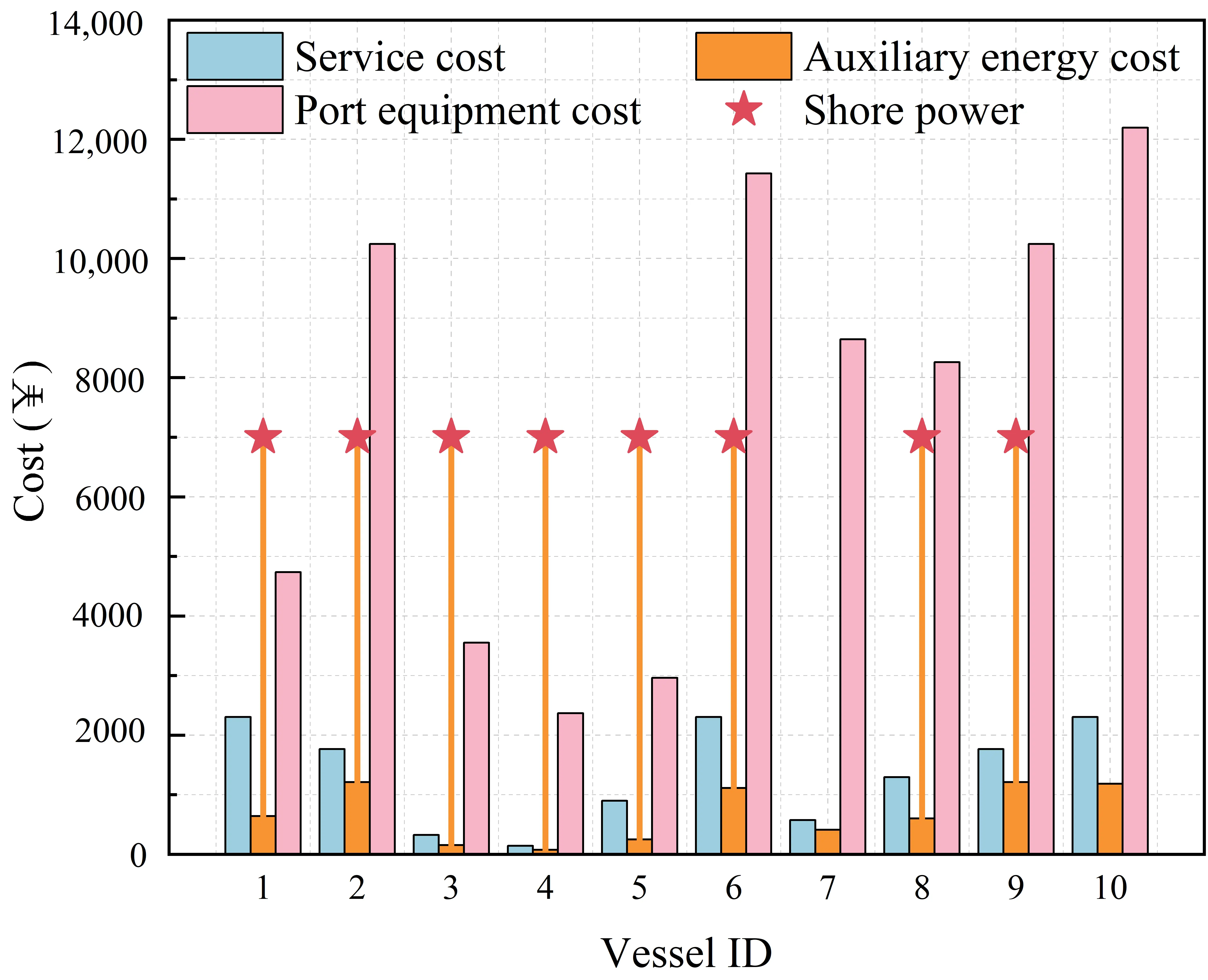
Figure 8 details the berthing costs of each ship before and after optimization. After optimization, the number of ships using shore power increased from 4 to 8. This is because the greedy strategy ignores energy price fluctuations and environmental costs, leading ships to be reluctant to connect to shore power during peak electricity price periods, resulting in a diesel usage proportion as high as 60%. In contrast, the CSA introduces a price-sensitive scheduling mechanism, enabling Ships 2, 3, 6, and 9 to independently choose to connect to shore power. This reduces both auxiliary engine energy costs and carbon emissions, achieving coordinated optimization of costs and carbon emissions. Additionally, in terms of port equipment costs, the optimized berth allocation scheme responds to TOU electricity pricing. For example, Ship 9 berths during off-peak electricity price periods, which not only reduces equipment idle loss but also lowers auxiliary engine energy costs by ¥49.03 and port equipment costs by ¥976.8. This verifies the superimposed effect of multi-objective optimization on cost control.

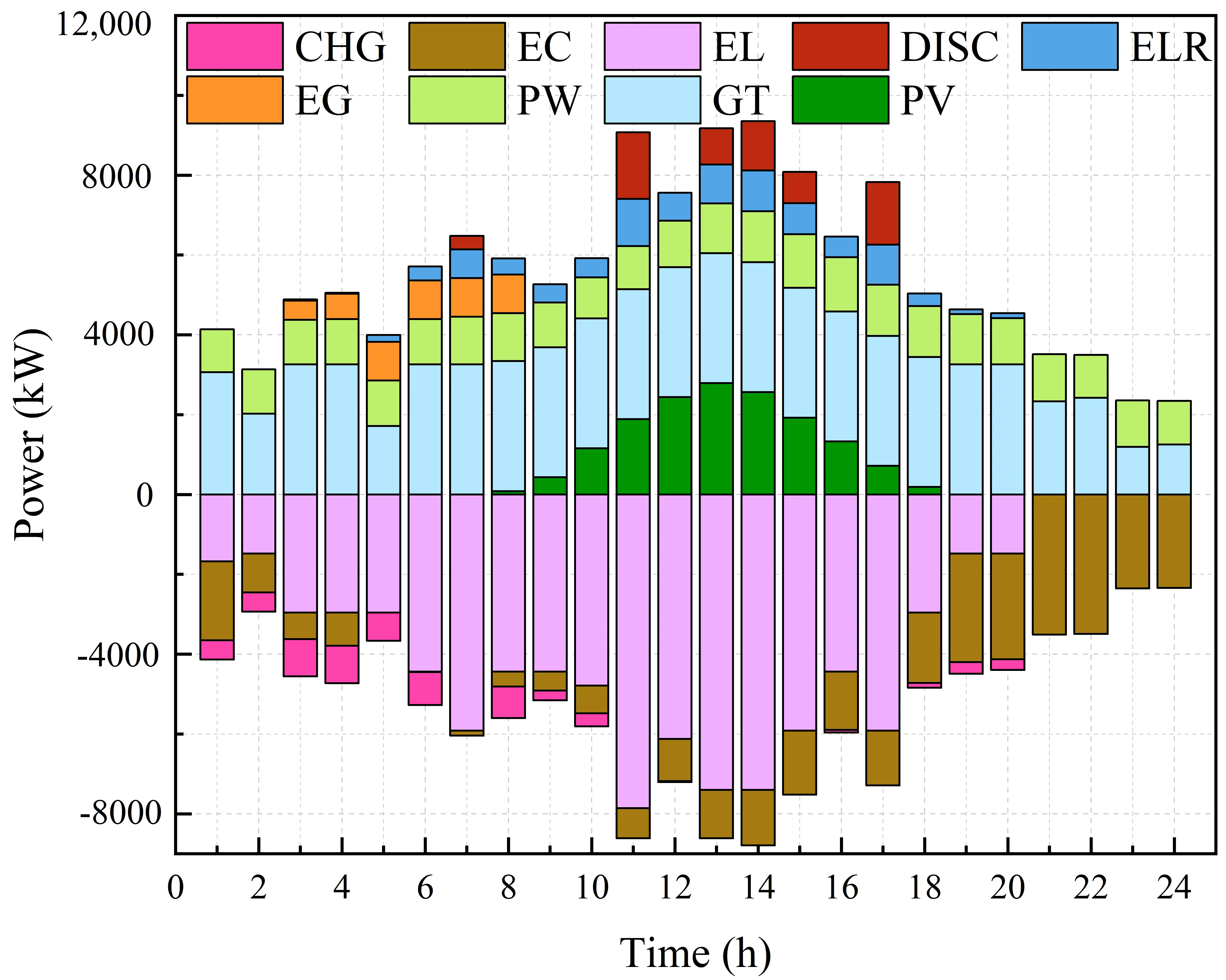
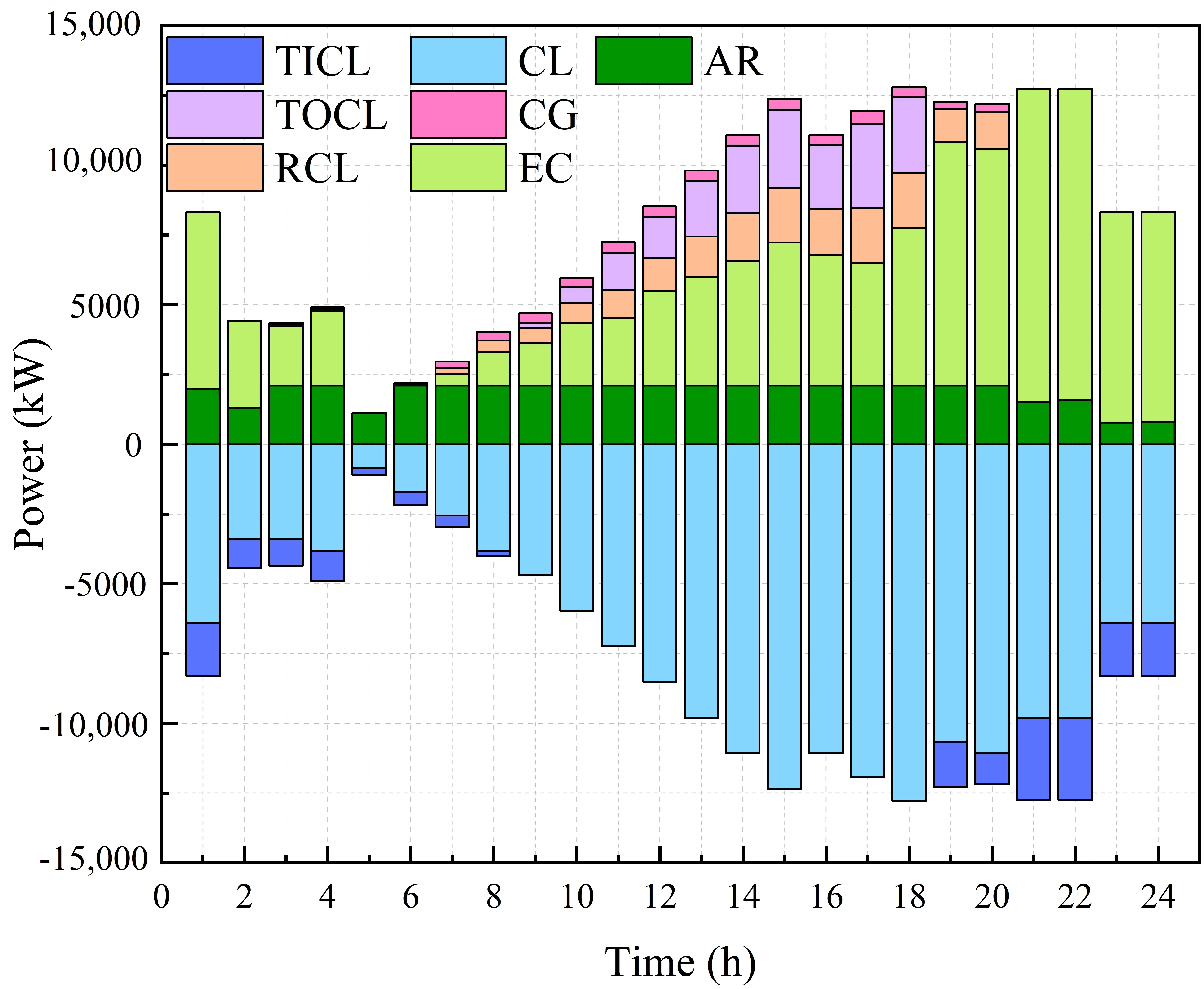
As shown in Figure 9, these are the power stack plots of various port equipment before and after optimization. Both plots exhibit the dynamic fluctuation characteristics of port operations over time, but their patterns differ significantly. The pre-optimization curve shows a pattern of high slope and narrow bandwidth, while the post-optimization curve presents a pattern of low slope and wide bandwidth. Additionally, a significant peak appears between 10:00 and 14:00 before optimization, with the peak total power reaching approximately 9000 kW. After optimization, the peak period shifts from 11:00 to 15:00, and the peak power is significantly lower than that before optimization. This indicates that different berth allocation schemes result in different operating patterns of port equipment. Electricity consumption is more concentrated throughout the day before optimization. However, a certain degree of peak shaving and shifting is achieved during peak electricity usage periods after optimization, which helps alleviate the peak regulation pressure on distributed energy equipment.

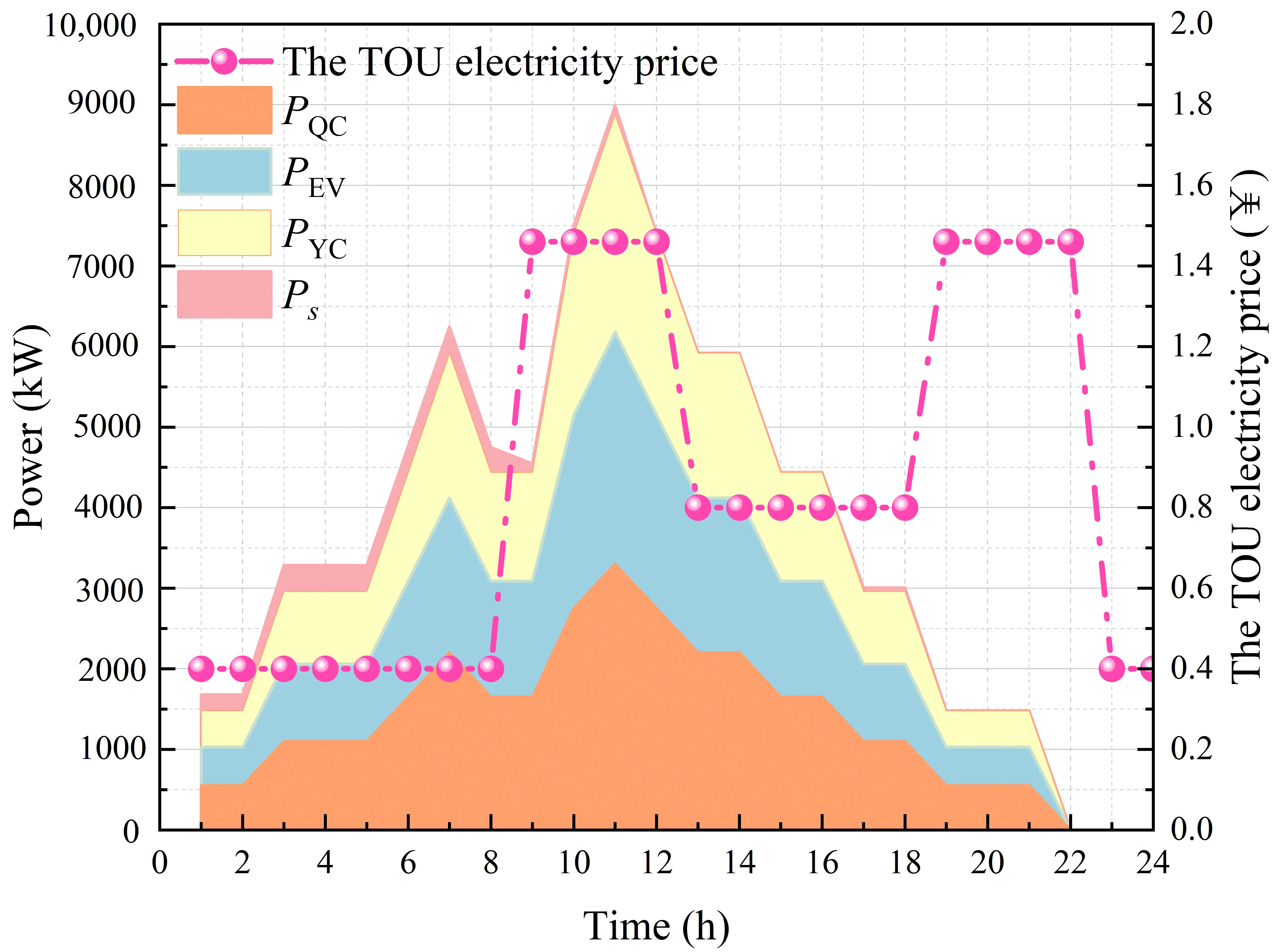
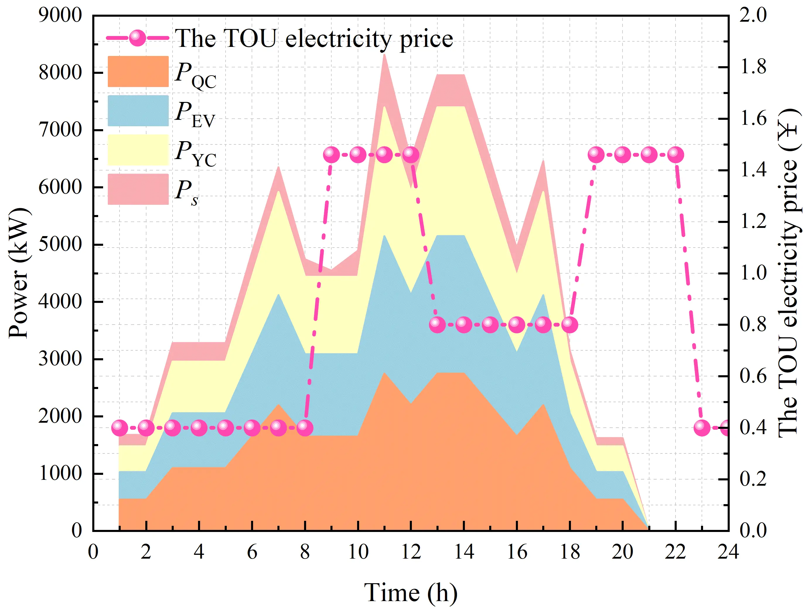
Additionally, the power of various port equipment determined by the berth allocation in the first stage acts as a bridge for the two-stage optimization. It is input into the Stackelberg game as the load parameters of the PEA in the second stage to optimize the port energy system.

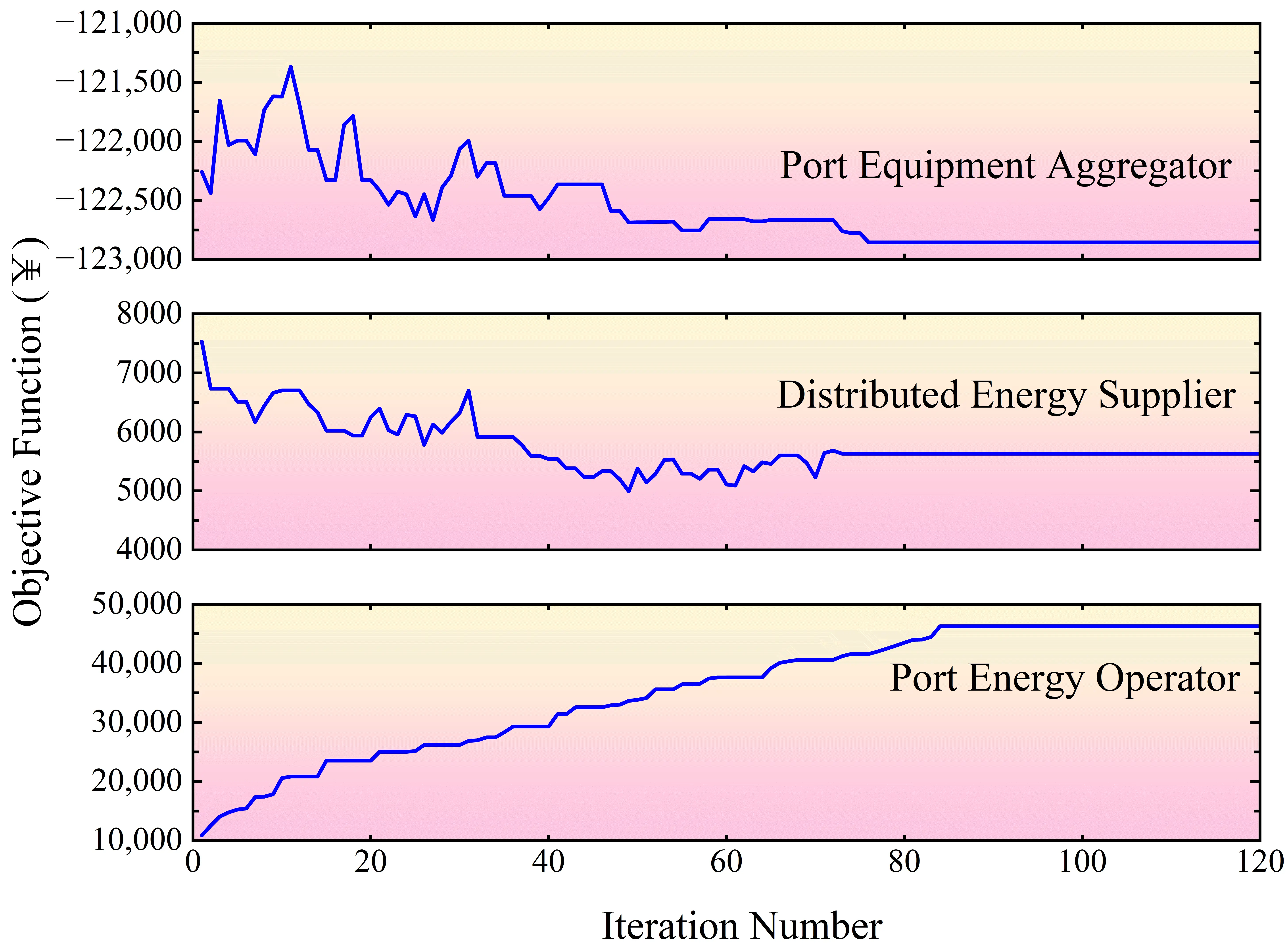
The iteration curves of the objective functions for the three entities under the Stackelberg game model are shown in Figure 10. During the game process, the PEO dynamically adjusts prices based on the load demand of the PEA and the energy supply capacity of the DES, driving the progression of the Stackelberg game. The final stable state indicates that the PEO’s pricing strategy has reached equilibrium, achieving coordinated optimization among the three port entities.

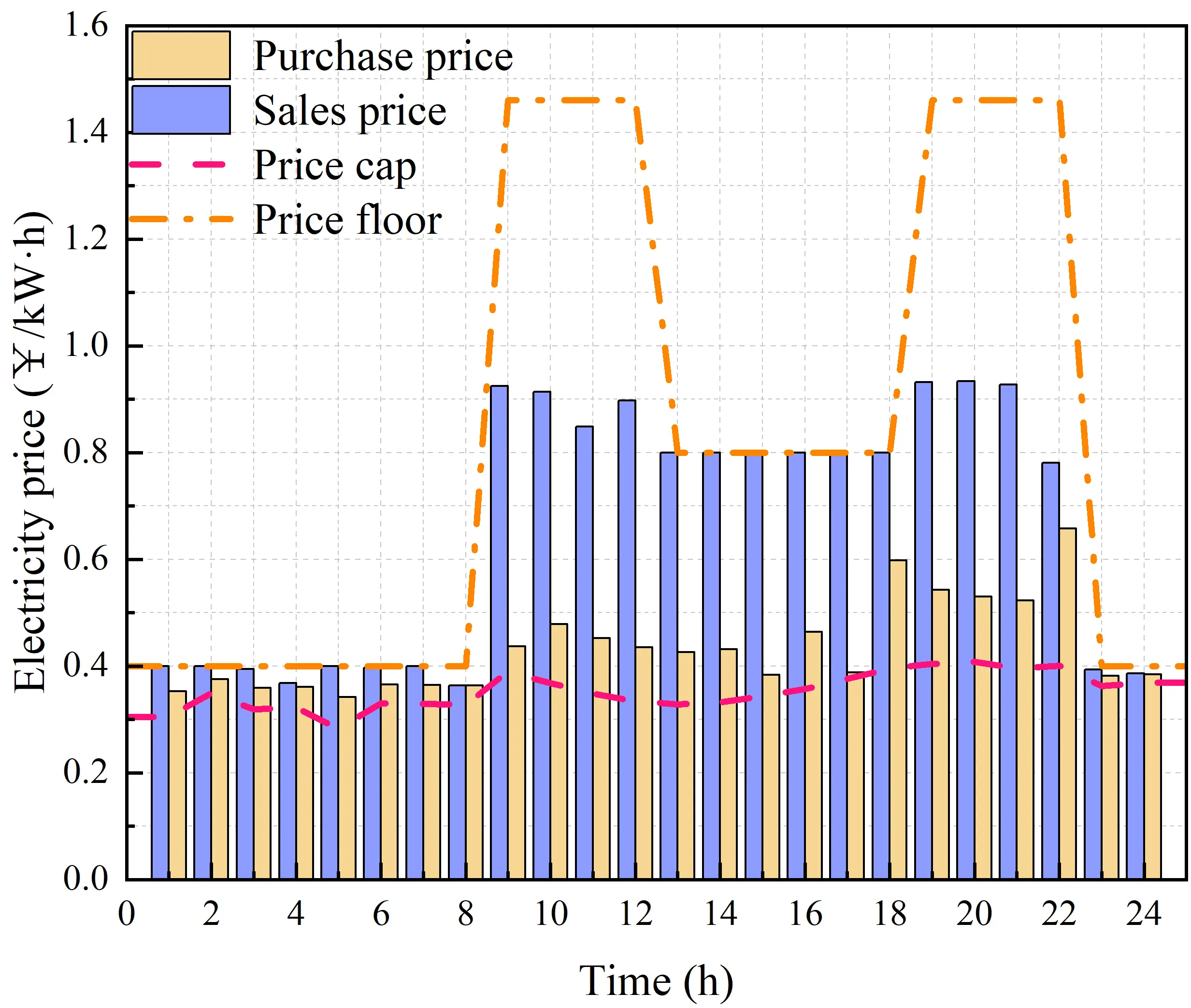
Under the Stackelberg game mechanism, the buying and selling prices of the port electricity and cooling energy have been precisely optimized. As shown in Figure 11, the buying and selling prices of electricity and cooling energy fall between the prices of the upper-level energy networks and the cost prices. This not only ensures the revenue of the DES from energy sales to the PEO but also endows the price at which the PEO sells energy to the PEA with market competitiveness.

When the TOU electricity price is in the off-peak period (23:00–8:00), the margin between it and the cost-based electricity price is small. This makes the optimized electricity selling price of the PEO very close to the TOU electricity price, and the PEO’s revenue is low during this period. When the TOU electricity price is in the peak period (9:00–12:00 and 19:00–22:00), the cost-based electricity price changes little compared with the other periods. So, the gap between the PEO’s electricity purchasing and selling prices is significant, and the PEO’s revenue is relatively high. When the TOU electricity price is in the flat-rate period (13:00–18:00), analysis of the load curve indicates that the PEA’s equipment operates intensively during this time, leading to high electric load demand. To regulate the peak electric load while pursuing revenue, the PEO maintains its electricity selling price at a high level, roughly equal to the TOU electricity price. The cooling energy price follows a similar variation pattern to the electricity price; thus, cooling energy prices follow a trend of first decreasing and then increasing in response to changes in cooling load.

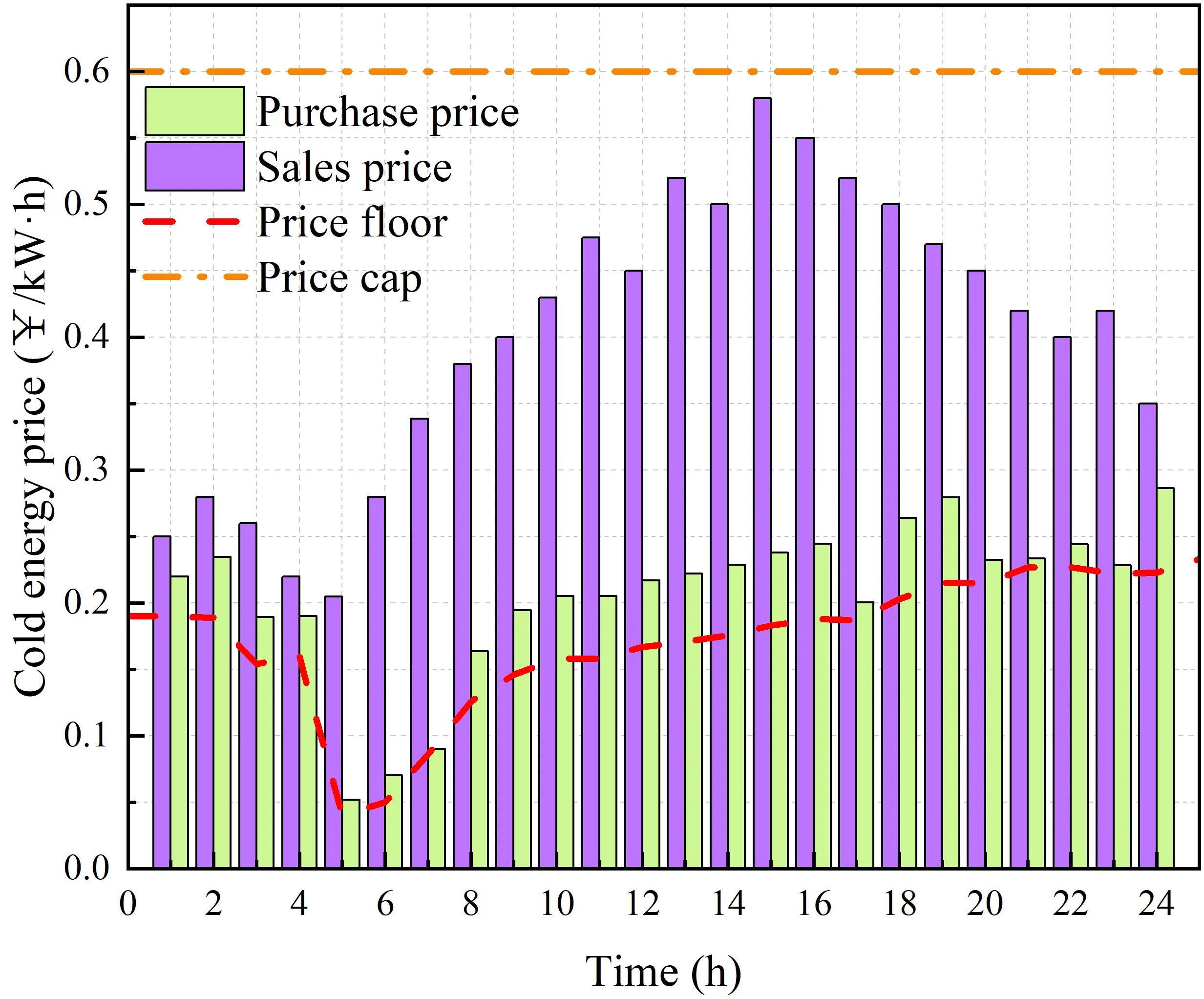
As shown in Figure 12, the electric load of the PEA has achieved effective peak shaving and valley filling. During the peak period (10:00–16:00), the electric load drops sharply from nearly 8000 kW to approximately 5500 kW, alleviating the peak pressure on the power grid. During off-peak periods, the load is moderately increased, which not only improves energy utilization efficiency but also reduces costs by purchasing electricity at off-peak prices. In addition to peak shaving and valley filling, the cooling load also exhibits the characteristics of peak shifting. Since part of the peak refrigeration load is provided by electric chillers, shifting the cooling load from the peak period (13:00–18:00) to the off-peak period of electric load (19:00–1:00) effectively reduces the operating pressure on the port’s cooling and electricity systems during peak periods.

The coordinated optimization of the two forms a positive interaction: the optimization of electric load provides power support for the adjustment of the cooling energy system, and the optimization of cooling load in turn promotes the stable operation of the electric load.

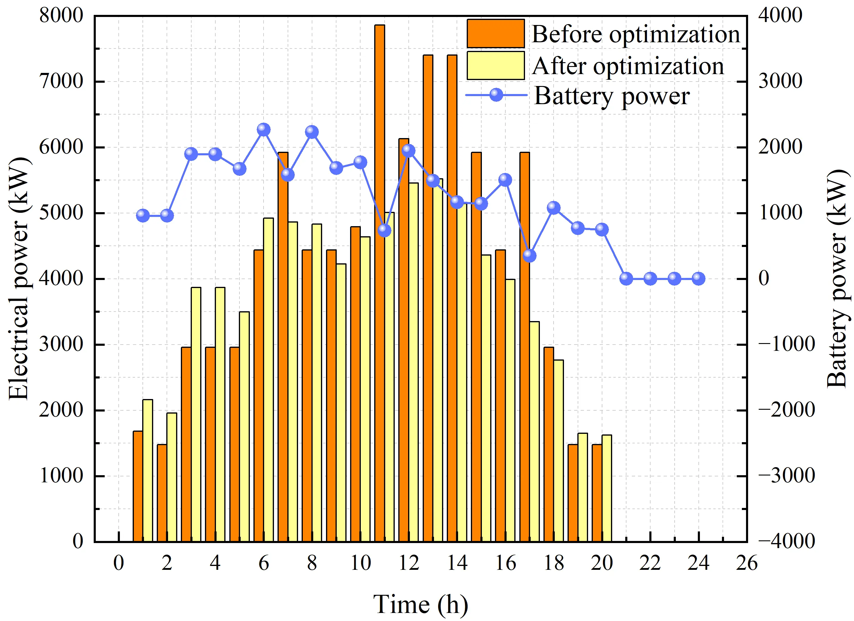
The coordinated operation of the DES equipment under the Stackelberg game is shown in Figure 13. The electric load side regulates the electric load through load curtailment and the charging-discharging control of the SBEV’s batteries. The electric load consumed by the ECs presents an obvious peak-shifting pattern compared with the original electric load, which avoids the occurrence of superimposed electric load peaks and helps ensure the stability of the power supply.

Secondly, as light intensity increases (8:00–15:00), the PV units start contributing output. Meanwhile, the SBEV’s batteries are charged during off-peak electricity periods and discharged during peak periods, leveraging the economic benefits of low-cost charging and high-price discharging of truck batteries. These factors constitute a decrease in the output of GTs during this period. However, during periods of the low TOU electricity prices (3:00–8:00), since the cooling load is in the off-peak period at the time, high-power operation of combined cooling and power units will result in cooling energy waste. Therefore, partial output from the upper-level power grid is encouraged to meet the electric load during this period.

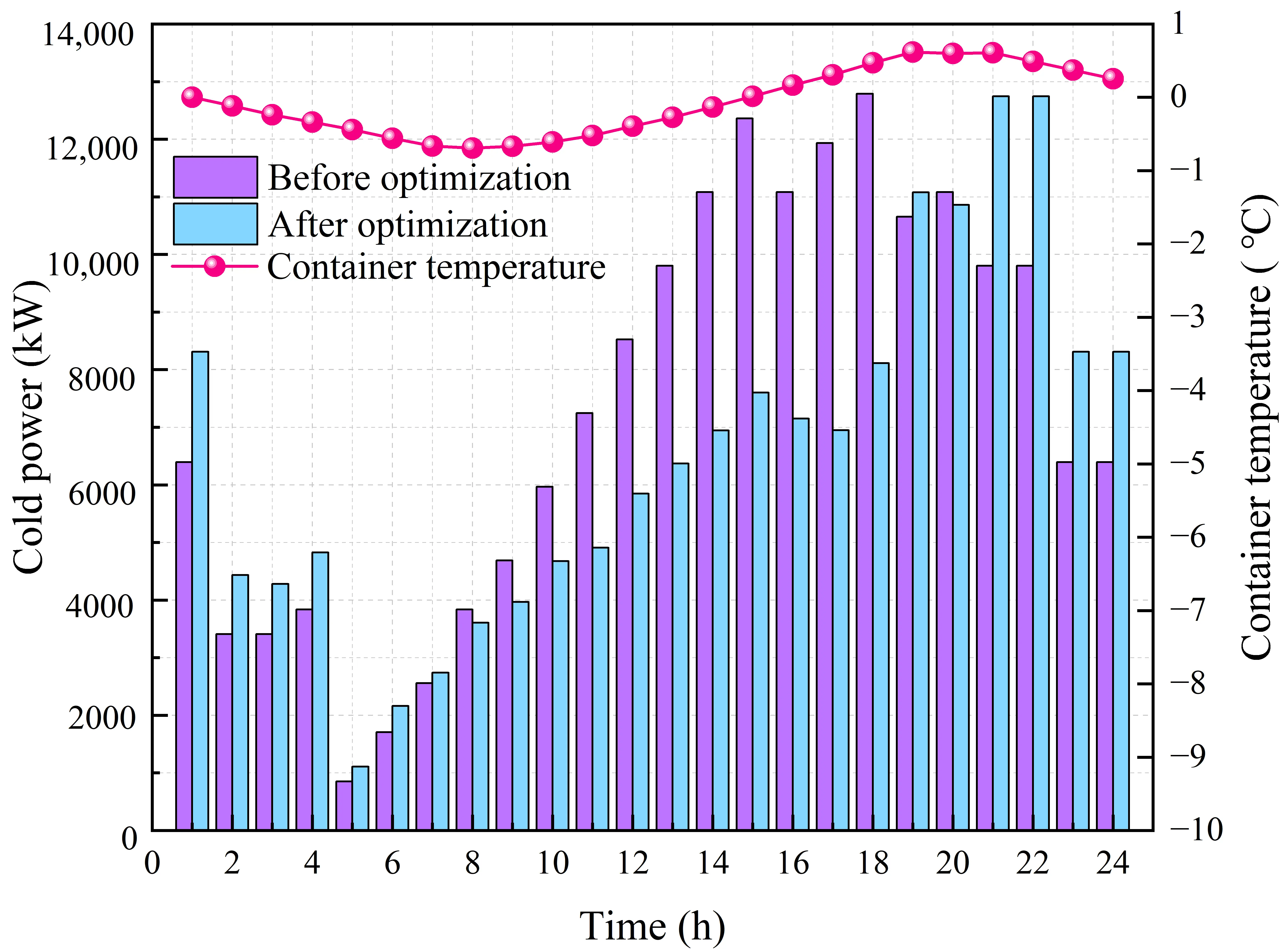
The equipment output of the DES to meet the cooling load is relatively simple, mainly relying on the ARs and ECs. During the peak electric load period (8:00–18:00), to reduce the power consumption of the ECs, energy supply from the upper-level refrigeration network is used as a supplement.

To validate the effectiveness of the port energy system modeling and optimization approach proposed in the paper, four analytical scenarios were established for examination. Detailed descriptions of these scenarios are provided in Table 5.

As shown in Table 6, the four scenarios exhibit a trend of progressive optimization in terms of cost and carbon emissions. In Scenario 1, energy is fully supplied by the upper-level energy networks, with a total cost of ¥175,149.9. Since the energy from the upper-level networks is mainly generated by coal, carbon emissions remain high. In Scenario 2, a tripartite game is conducted through the Stackelberg game mechanism, and the DES is introduced for low-carbon energy supply. As a result, the total cost decreases to ¥123,789.51, and carbon emissions are reduced by over 75%. Scenario 3 introduces the DRLM, considering SBEV’s battery swapping, realizing peak shifting and valley filling of the load, and further responding to TOU electricity pricing. Part of the electric load relies on the upper-level power grid for peak regulation, leading to a slight increase of 2% in carbon emissions. Scenario 4 imposes further constraints on carbon emissions. Carbon emissions generated from electricity and cooling energy are incorporated into costs as a penalty, with a focus on prioritizing the use of local low-carbon energy. While the total cost increases slightly by 0.09%, carbon emissions are reduced by 13%. In summary, the progressive comparison of the four scenarios demonstrates the synergistic optimization path for the port’s economic efficiency and low-carbon performance.

Based on the improved CSA and Stackelberg game theory, the study establishes a two-stage optimization framework to conduct collaborative optimization of the port berth allocation and energy system optimization. By designing multiple scenarios, the effectiveness of the models and methods proposed in the study is verified. The main conclusions are as follows:

This study establishes a two-stage optimization framework for port berth allocation and marine energy utilization based on the Improved Cuckoo Search Algorithm (ICSA) and the Stackelberg game, and verifies its effectiveness through a case study. However, given the focus on the core logic of collaborative optimization between port logistics and energy systems, the current research has certain limitations in considering actual operational environmental factors and algorithm application scenarios, which are mainly reflected in the following aspects: The model fails to account for the impacts of meteorological factors (e.g., typhoons, rainstorms, heavy fog, extreme temperatures) and hydrodynamic factors (e.g., sea level rise, ocean current velocity, wave height) on port operations and offshore energy output. In actual port operations, extreme weather directly affects ship arrival time, berthing safety, and the operational efficiency of port electromechanical equipment. Hydrodynamic factors and weather variations also significantly influence the power generation stability of offshore wind power and offshore photovoltaic systems.

To address the limitations, follow-up research will focus on algorithm improvement and model expansion to further enhance the practical application value of the optimization framework, mainly including: Integrating meteorological and hydrodynamic factors into the optimization model: Long-term marine environmental monitoring data (meteorology, ocean currents, waves, water temperature, etc.) in the port area will be collected to construct an impact model of environmental factors, which will be coupled with the existing two-stage optimization framework. On the one hand, a marine energy output prediction model considering environmental factors will be established to improve the accuracy of offshore wind and photovoltaic power output forecasting. On the other hand, environmental constraints will be added to the berth allocation model to optimize the berth allocation scheme in real time according to environmental changes and adaptively adjust the port energy load curve.

Q.G.: Writing—review & editing, Project administration, Formal analysis. L.G.: Writing—review & editing, Writing—original draft, Visualization, Software, Methodology. Z.B.: Writing—review & editing, Resources, Data curation. L.Z.: Writing—review & editing, Resources, Formal analysis, Project administration. J.L.: Writing—review & editing, Data curation. Y.S.: Writing—review & editing, Supervision, Methodology. Y.J.: Writing—review & editing, Methodology, Visualization, Software. X.G.: Writing—review & editing, Methodology.

Not applicable for studies not involving humans or animals.

Not applicable for studies not involving humans.

Data will be made available on request.

This work was supported by the top-level project of the National Natural Science Foundation of China (No.52077150), the Natural Science Foundation of Tianjin (No.24JCYBJC00280), the Research and Reform Fund for Postgraduate Education and Teaching of Tianjin University of Technology (No.ZDXM2502), the science and technology projects of State Grid Tianjin Electric Power Company: “Electricity-Heat Integrated Energy System Flexibility and Reliability” (No.H20210063), “Research on Energy Global Optimization and Interactive Adjustment Technique for Urban Building Bodies Based on Multi-source Data Fusion” (No.KJ21-1-21).

The authors declare that they have no known competing financial interests or personal relationships that could have appeared to influence the work reported in this paper.

References

- Tang E, Gao J, Huang W, Qian Y. Marine renewable energy: Progress, challenges, and pathways to scalable sustainability. Energy 2025, 335, 138083. DOI:10.1016/j.energy.2025.138083 [Google Scholar]
- Alzahrani A, Petri I, Rezgui Y, Ghoroghi A. Decarbonisation of seaports: A review and directions for future research. Energy Strategy Rev. 2021, 38, 100727. DOI:10.1016/j.esr.2021.100727 [Google Scholar]
- Bullock S, Larkin A, Kähler J. Beyond fuel: The case for a wider perspective on shipping and climate change. Clim. Policy 2025, 25, 1326–1334. DOI:10.1080/14693062.2024.2447474 [Google Scholar]
- Wan Z, Nie A, Chen J, Pang C, Zhou Y. Transforming ports for a low-carbon future: Innovations, challenges, and opportunities. Ocean Coast. Manag. 2025, 264, 107636. DOI:10.1016/j.ocecoaman.2025.107636 [Google Scholar]
- Zheng H, Wang Z, Fan X. Integrated rescheduling optimization of berth allocation and quay crane allocation with shifting strategies. Ocean Eng. 2024, 301, 117473. DOI:10.1016/j.oceaneng.2024.117473 [Google Scholar]
- Gabrielii C, Gammelsæter M, Mehammer EB, Damman S, Kauko H, Rydså L. Energy systems integration and sector coupling in future ports: A qualitative study of Norwegian ports. Appl. Energy 2025, 380, 125003. DOI:10.1016/j.apenergy.2024.125003 [Google Scholar]
- Iris Ç, Lam JSL. A review of energy efficiency in ports: Operational strategies, technologies and energy management systems. Renew. Sustain. Energy Rev. 2019, 112, 170–182. DOI:10.1016/j.rser.2019.04.069 [Google Scholar]
- Elkafas AG, Seddiek IS. Application of renewable energy systems in seaports towards sustainability and decarbonization: Energy, environmental and economic assessment. Renew. Energy 2024, 228, 120690. DOI:10.1016/j.renene.2024.120690 [Google Scholar]
- Parhamfar M, Sadeghkhani I, Adeli AM. Towards the application of renewable energy technologies in green ports: Technical and economic perspectives. IET Renew. Power Gener. 2023, 17, 3120–3132. DOI:10.1049/rpg2.12811 [Google Scholar]
- Lyu X, Lalla-Ruiz E, Schulte F. The collaborative berth allocation problem with row-generation algorithms for stable cost allocations. Eur. J. Oper. Res. 2025, 323, 888–906. DOI:10.1016/j.ejor.2024.12.048 [Google Scholar]
- Al Samrout M, Sbihi A, Yassine A. An improved genetic algorithm for the berth scheduling with ship-to-ship transshipment operations integrated model. Comput. Oper. Res. 2024, 161, 106409. DOI:10.1016/j.cor.2023.106409 [Google Scholar]
- Aslam S, Michaelides MP, Herodotou H. Berth allocation considering multiple quays: A practical approach using cuckoo search optimization. J. Mar. Sci. Eng. 2023, 11, 1280. DOI:10.3390/jmse11071280 [Google Scholar]
- Song Y, Ji B, Yu SS. Multi-port berth allocation and time-invariant quay crane assignment problem with speed optimization. IEEE Trans. Intell. Transp. Syst. 2025, 26, 128–142. DOI:10.1109/TITS.2024.3481490 [Google Scholar]
- Peng Y, Dong M, Li X, Liu H, Wang W. Cooperative optimization of shore power allocation and berth allocation: A balance between cost and environmental benefit. J. Clean Prod. 2021, 279, 123816. DOI:10.1016/j.jclepro.2020.123816 [Google Scholar]
- Pu Y, Liu H, Wang J, Hou Y. Collaborative scheduling of port integrated energy and container logistics considering electric and hydrogen-powered transport. IEEE Trans. Smart Grid 2023, 14, 4345–4359. DOI:10.1109/TSG.2023.3266601 [Google Scholar]
- Li B, Elmi Z, Manske A, Jacobs E, Lau YY, Chen Q, et al. Berth allocation and scheduling at marine container terminals: A state-of-the-art review of solution approaches and relevant scheduling attributes. J. Comput. Des. Eng. 2023, 10, 1707–1735. DOI:10.1093/jcde/qwad075 [Google Scholar]
- Ma K, Feng Y, Yang J, Cai Y, Yang B, Guan X. Two-stage distributionally robust optimization for port integrated energy system with berth allocation under uncertainties. Energy 2025, 322, 135588. DOI:10.1016/j.energy.2025.135588 [Google Scholar]
- Pu Y, Liu H, Wang J, Xu Y, Anvari-Moghaddam A. Cooperative dispatching of port integrated energy and ferry logistics systems under interrelated cross-domain uncertainties. Energy 2025, 337, 138507. DOI:10.1016/j.energy.2025.138507 [Google Scholar]
- Ren F, Wei Z, Zhai X. A review on the integration and optimization of distributed energy systems. Renew. Sustain. Energy Rev. 2022, 162, 112440. DOI:10.1016/j.rser.2022.112440 [Google Scholar]
- Li J, Chen H, Qi Y, Wang Y, Lei J. Collaborative optimization for cross-regional integrated energy systems producing electricity-heat-hydrogen based on generalized Nash bargaining. Energy 2025, 333, 137444. DOI:10.1016/j.energy.2025.137444 [Google Scholar]
- Ma W, Tang D, Dong M, Arasteh H, Guerrero JM. Coordinated robust configuration of soft open point and energy storage systems for resilience enhancement of integrated multi-energy system at ports. Appl. Energy 2025, 401, 126644. DOI:10.1016/j.apenergy.2025.126644 [Google Scholar]
- Tang D, Ge P, Yuan C, Ren H, Zhong X, Dong M, et al. Optimal management of coupled hydrogen-electricity energy systems at ports by multi-time scale scheduling. Appl. Energy 2025, 391, 125885. DOI:10.1016/j.apenergy.2025.125885 [Google Scholar]
- Wang J, Cui Y, Liu Z, Zeng L, Yue C, Agbodjan YS. Multi-energy complementary integrated energy system optimization with electric vehicle participation considering uncertainties. Energy 2024, 309, 133109. DOI:10.1016/j.energy.2024.133109 [Google Scholar]
- Xie T, Ma K, Zhang G, Zhang K, Li H. Optimal scheduling of multi-regional energy system considering demand response union and shared energy storage. Energy Strategy Rev. 2024, 53, 101413. DOI:10.1016/j.esr.2024.101413 [Google Scholar]
- Astriani Y, Shafiullah GM, Shahnia F. Incentive determination of a demand response program for microgrids. Appl. Energy 2021, 292, 116624. DOI:10.1016/j.apenergy.2021.116624 [Google Scholar]
- Zhang J, Liu Z. Low carbon economic scheduling model for a park integrated energy system considering integrated demand response, ladder-type carbon trading and fine utilization of hydrogen. Energy 2024, 290, 130311. DOI:10.1016/j.energy.2024.130311 [Google Scholar]
- Wang K, Wang C, Yao W, Zhang Z, Liu C, Dong X, et al. Embedding P2P transaction into demand response exchange: A cooperative demand response management framework for IES. Appl. Energy 2024, 367, 123319. DOI:10.1016/j.apenergy.2024.123319 [Google Scholar]
- Zhang Y, Liang C, Shi J, Lim G, Wu Y. Optimal port microgrid scheduling incorporating onshore power supply and berth allocation under uncertainty. Appl. Energy 2022, 313, 118856. DOI:10.1016/j.apenergy.2022.118856 [Google Scholar]
- Mao A, Yu T, Ding Z, Fang S, Guo J, Sheng Q. Optimal scheduling for seaport integrated energy system considering flexible berth allocation. Appl. Energy 2022, 308, 118386. DOI:10.1016/j.apenergy.2021.118386 [Google Scholar]
- Li P, Dong Z, Ma K, Yang H. IGDT-based coordinated optimization for port berth-logistics-energy scheduling with electricity-hydrogen coupled transport. Energy 2025, 336, 138336. DOI:10.1016/j.energy.2025.138336 [Google Scholar]
- Zhou Y, Li Y, Huang W, Chen S, Zang H, Tai N. Collaborative scheduling of seaport integrated energy, logistics, and vessels: A bi-level nash-stackelberg-nash game approach. Appl. Energy 2025, 400, 126598. DOI:10.1016/j.apenergy.2025.126598 [Google Scholar]
- Shi S, Ji Y, Zhu L, Liu J, Gao X, Chen H, et al. Interactive optimization of electric vehicles and park integrated energy system driven by low carbon: an incentive mechanism based on Stackelberg game. Energy 2025, 318, 134799. DOI:10.1016/j.energy.2025.134799 [Google Scholar]
- Zhao S, Yao J, Li Z. A study on wind power scenario reduction method based on improved K-means clustering and SBR algorithm. Power Syst. Technol. 2021, 45, 3947–3954. [Google Scholar]