Buckling and Post-Buckling Behavior of the Delaminated Composite Plates

Buckling and Post-Buckling Behavior of the Delaminated Composite Plates
Lubov Bokhoeva 1,2,3,* Vitaly Rogov 4 Shunqi Mei 3 Anna Chermoshentseva 5 Anatoly Ivanov 1 Alexander Nadtochin 1
Received: 08 December 2025 Revised: 09 January 2026 Accepted: 02 February 2026 Published: 06 February 2026

© 2026 The authors. This is an open access article under the Creative Commons Attribution 4.0 International License (https://creativecommons.org/licenses/by/4.0/).
1. Introduction
Interest in the use of composite materials has now increased. Multilayer composite materials with high specific strength and rigidity are sensitive to interlayer defects. Delamination is the most common type of defect and is often considered a determining factor in deciding the use of composites in structures. Delamination may occur at stress concentrations or in the area of abrupt changes in material thickness, as a result of imperfections in production technology or the action of operational loads [1,2].
The tasks of studying the plate with interlayer defects during axial compression have received a lot of attention since the 1980s, starting with the work of Chai and colleagues [3,4]. A large number of studies of this problem mainly determine the critical load [5,6,7,8,9,10,11,12].
When the critical load is reached, three types of buckling of structural elements made of composite materials with delamination defects are possible [9,13]. The first type of buckling is the global buckling of the entire plate, the buckling of the composite beam as a whole. It is observed with defects of short length. The second type of buckling is local bulging of the defect; the remaining parts of the plate remain flat. Local buckling is the main type of compression failure of laminated composites with thin lamination defects. The third type of buckling is called “mixed”, in which both local and global buckling are possible when the defect and the rest of the plate are bent.
The objectives of studying the supercritical behavior of a local interlayer defect occurring in a plate are proposed in [5,6,8,9,12]. A post-buckling study for a plate supported on all edges and containing an embedded lamination can be found in [10,11,12,14]. However, only Ref. [8] considers a non-rectangular, elliptical delamination shape. Information in the literature on post-buckling behavior for elliptically delaminated composite plates is rare. In addition, the problem of a composite plate with embedded lamination loaded by axial compression is mainly studied using the finite element method. Thus, analytical approaches to modeling are lacking.
This work examines the behavior after the loss of stability of an elliptical defect in a composite plate. Only the local bulging of the delamination type defect was considered. The difference between this work and others lies in the fact that the application of the developed method, based on the energy approach, makes it possible to obtain explicit analytical expressions for quantities characterizing the critical load and describing the supercritical behavior of the detached part. The energy method is generalized to the case of analyzing the stability of defects in a non-linear formulation. The value of the critical load was obtained and the analysis of the supercritical deformation of the defect was made.
2. Development and Modeling
In the cycle of strength calculations, stability calculations play an essential role, since the failure of thin-walled structural elements during compression is usually associated with a loss of general or local stability [5,6,7,8,9,10]. Consider of a delaminated composite plate subjected to in-plane compressive loading $${\epsilon }_{x}$$,$${\epsilon }_{y}$$ (Figure 1). The center of the defect coincides with the origin of the oxy coordinates. We will consider the defect as a thin axisymmetric plate, pinched along the contour and subjected to a uniformly distributed load with an intensity $${q}_{x}$$,$${q}_{y}$$ corresponding to the main load of the structural element. Forces corresponding to warp deformations are set along the defect contour $${\epsilon }_{x}$$,$${\epsilon }_{y}$$,
| $${q}_{x}=\frac{{\epsilon }_{x}{E}_{x}h}{1-{\mu }_{xy}}$$; $$\,\,\,\,$$$${q}_{y}=\frac{{\epsilon }_{y}{E}_{y}h}{1-{\mu }_{yx}}$$. |
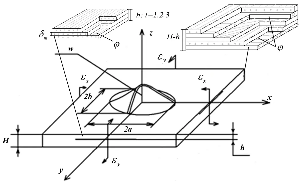
Figure 1. А composite plate with delamination, loaded with compressive deformations at the ends $${\epsilon }_{x}$$,$${\epsilon }_{y}$$.
For thin-walled multilayer structural elements, a plane stress state and bending are typical [6,7,8,9]. The boundaries of the local bundle are given by the equation
| ```latex\frac{{x}^{2}}{{a}^{2}}+\frac{{y}^{2}}{{b}^{2}}=1,``` |
the semi–axes of the bundle are a and b, h is the thickness of the bundle. In addition, h satisfies the condition h << a, b. In the region of stratification, a multilayer plate consists of two parts (Figure 1): a stratified layer (upper part h) and a layer located below the stratification (lower part is thick H-h). The main part of the laminated plate with thickness H is located outside the defect. The plate consists of n layers, t—number of lamination layers, $${\delta }_{m}$$—thickness of m—one layer, m—number of layers.
The behavior of multilayer composite materials under load, even with a linear dependence of deformations on stresses, is fundamentally different from the behavior of isotropic [7,8]. To determine the elastic characteristics of a multilayer plate package and local stratification, we use the relations for unidirectional material that reflect the contribution of each component in proportion to its volume fraction, the so-called “mixture rule” [9,10]. Let’s imagine a unidirectional composite material (OKM) in the form of alternating layers with matrix and fiber properties. Then $$f_{\textit{в}}$$ + $$f_{\textit{м}}$$ = 1, where $$f_{\textit{в}}$$ the relative volume content of fiber in the OKM, $$f_{\textit{м}}$$ is the relative volume content of matrix in the OKM. Using a JSM-6510LV JEOL scanning electron microscope (JEOL Ltd., Tokyo, Japan), the volume fraction of fiber $$f_{\textit{в}}$$ (Figure 2) for glass fiber d = 6 µm was determined, the fraction of which is 0.7 (percentage of fiber—70%).
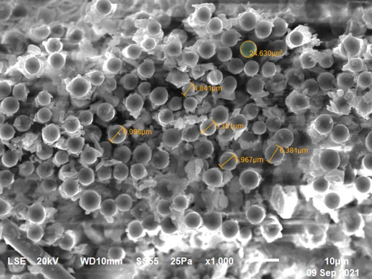
Figure 2. Cross-section image of a single fiber. Accelerating voltage: 20 kV, WD:10 mm, detector: S355, mode (25 Pa) magnification 1000.
The elastic characteristics of the fiber and matrix for OCM are shown in Table 1.
Table 1. Elastic characteristics of the fiber and matrix.
|
Elastic Characteristics of Fiberglass |
Elastic Characteristics of the Epoxy Matrix |
|---|---|
|
$$E_{\textit{в}}$$ = 7.3 × 10⁴ MPa |
E$$_{\textit{м}}$$ = 3.78 × 10³ MPa |
|
$$G_{\textit{в}}$$ = 2.9 × 10⁴ MPa |
G$$_{\textit{м}}$$ = 1.4 × 10³ MPa |
|
µ$$_\textit{в}$$ = 0.22 |
µ$$_{\textit{м}}$$ = 0.35 |
We find the values of the elastic constants OKM in terms of the elastic constants and the volume fractions of the components using the following expressions:
| ```latex\begin{aligned}&{E}_{1}={f}_{\textit{в}}{\mu }_{\textit{в}}+{f}_{\textit{м}}{\mu }_{\textit{м}}\\&{E}_{2}=\frac{{E}_{\textit{в}}{E}_{\textit{м}}{E}_{1}}{{E}_{1}\left[{f}_{\textit{в}}{E}_{\textit{м}}+{f}_{\textit{м}}{E}_{\textit{в}}\right]-{f}_{\textit{в}}{f}_{\textit{м}}{\left({\mu }_{\textit{м}}{E}_{\textit{в}}-{\mu }_{\textit{в}}{E}_{\textit{м}}\right)}^{2}}\\&{G}_{12}=\frac{{G}_{\textit{в}}{G}_{\textit{м}}}{{f}_{\textit{в}}{G}_{\textit{м}}+{f}_{\textit{м}}{G}_{\textit{в}}}\\&{\mu }_{12}={f}_{\textit{в}}{\mu }_{\textit{в}}+{f}_{\textit{м}}{\mu }_{\textit{м}}\\&{\mu }_{21}=\frac{{\mu }_{12}{E}_{2}}{{E}_{1}}\end{aligned}``` | (1) |
where E1 is the modulus of elasticity along the reinforcement direction, E2 is the modulus of elasticity across the reinforcement direction, G12 is the shear modulus in the layer plane, $$\mu_{12},\mu_{21}$$ and are the coefficients of transverse deformations. The elastic constants for OKM, according to relations (1), are presented in Table 2. The analytical values are refined through numerical calculations in the Ansys Mechanical software package (Ansys 2024 R2).
Table 2. Elastic characteristics of OKM.
|
The Elastic Characteristics of OKM (Fiberglass) Are Obtained by the Ratios (1) |
The Elastic Characteristics of OKM (Fiberglass) Were Obtained in the Ansys Mechanical Software Package. |
|---|---|
|
E1 = 5.223 × 10⁴ MPa |
E1 = 5.225 × 10⁴ MPa |
|
E2 = 1.124 × 10⁴ MPa |
E2 = 1.759 × 10⁴ MPa |
|
G12 = 4.207 × 10³ MPa |
G12 = 4.459 × 10⁴ MPa |
|
µ21 = 0.259 |
µ21 = 0.253 |
The elastic characteristics of a multilayer package are determined if the stiffness characteristics of the individual layers included in it are known: $$C_{j,s}^m$$—the stiffness characteristics of the 1st layer, depending on the elastic modulus, shear modulus, Poisson coefficients and the angle of orientation of the fibers of the unidirectional layer $${E}_{1},{E}_{2},{G}_{12},{\mu }_{12},{\mu }_{21},\varphi$$ ($$\varphi$$—the angle of orientation of the fibers of the layer). Expressions for the stiffness characteristics of the layer were obtained on the basis of [15,16]
| ```latex\begin{aligned}&C_{11}^m=&&\lambda(E_1\cos^4\varphi+E_2\sin^4\varphi+\frac{1}{2}\mu_{12}E_2\sin^22\varphi)+G_{12}\sin^22\varphi;\\&C_{22}^m=&&\lambda(E_1\sin^4\varphi+E_2\cos^4\varphi+\frac{1}{2}\mu_{12}E_2\sin^22\varphi)+G_{12}\sin^22\varphi;\\&C_{12}^m=&&\lambda[(E_1+E_2)\sin^2\varphi\cos^2\varphi+\mu_{12}E_2(\cos^4\varphi+\sin^4\varphi)]-G_{12}\sin^22\varphi;\\&C_{13}^m=&&[\frac{\lambda}{2}(E_{2}\sin^{2}2\varphi-E_{1}\cos^{2}2\varphi+\mu_{12}E_{2}\cos2\varphi)+G_{12}\cos2\varphi]\sin2\varphi;\\&C_{23}^{m}=&&[\frac{\lambda}{2}(E_{2}\cos^{2}2\varphi-E_{1}\sin^{2}2\varphi-\mu_{12}E_{2}\cos2\varphi)-G_{12}\cos2\varphi]\sin2\varphi;\\&C_{33}^{m}=&&\frac{\lambda\sin^22\varphi}{4}(E_1+E_2-2\mu_{12}E_2)+G_{12}\cos^22\varphi;\\&\lambda=&&\frac{1}{1-\mu_{12}\mu_{21}};E_{1}\mu_{21}=E_{2}\mu_{12}.\end{aligned}``` | (2) |
Let us consider the case of a local loss of stability, when the loss of stability begins with the bulging of a thin bundle. With sufficient accuracy for engineering calculations, it is possible to calculate the elastic characteristics of a multilayer composite material for layering (upper part):
| ```latexA_{11}=\frac{1}{h}\sum_{m=1}^t\delta_mC_{11}^m;A_{_{11}}=\frac{1}{h}\sum_{m=1}^t\delta_mC_{_{11}}^m;A_{_{22}}=\frac{1}{h}\sum_{m=1}^t\delta_mC_{_{22}}^m;\\E_{_x}=A_{_{11}}-\frac{A_{_{12}}^2}{A_{_{22}}};E_{_y}=A_{_{22}}-\frac{A_{_{12}}^2}{A_{_{11}}};\mu_{_{xy}}=\frac{A_{_{12}}}{A_{_{22}}};\mu_{_{yx}}=\mu_{_{xy}}\frac{E_{_y}}{E_{_x}};``` | (3) |
where $${E}_{x}$$ is the modulus of elasticity along the reinforcement direction for a package of multilayer composite material, thickness h; $${E}_{y}$$ is the modulus of elasticity across the reinforcement direction for a package of multilayer composite material, thickness h; $${\mu }_{xy},{\mu }_{yx}$$ are the coefficients of transverse deformation for a package of multilayer composite material, thickness h. Table 3 shows the values of the elastic characteristics of a multilayer composite material for layering (upper part) for two [0/90], three [0/90/0], four [0/90]2 layers of fiberglass (t = 2; 3; 4) [17,18].
Table 3. Elastic characteristics of elastic characteristics of multilayer composite material.
|
Layer Reinforcement Angle |
Stiffness Characteristics of the m-Layer, MPa |
||||||||
|---|---|---|---|---|---|---|---|---|---|
|
$${\bm{C}}_{11}^{\bm{m}}$$ |
$${\bm{C}}_{22}^{\bm{m}}$$ |
$${\bm{C}}_{12}^{\bm{m}}$$ |
$${\bm{C}}_{13}^{\bm{m}}$$ |
$${\bm{C}}_{23}^{\bm{m}}$$ |
$${\bm{C}}_{33}^{\bm{m}}$$ |
||||
|
m = 1 $$\varphi =0$$ |
5.223 × 10⁴ |
1.124 × 10⁴ |
3.148 × 10³ |
0 |
0 |
4.207 × 10³ |
|||
|
m = 0 $$\varphi =90$$ |
1.124 × 10⁴ |
5.223 × 10⁴ |
3.148 × 10³ |
3.906 × 10⁻¹² |
1.962 × 10⁻¹⁴ |
4.207 × 10³ |
|||
|
Elastic characteristics of a two-layer bundle [0/90] |
|||||||||
|
|
|
```latex{\mu }_{xy}``` |
```latex{\mu }_{yx}``` |
||||||
|
2.095 × 10⁴ |
2.095 × 10⁴ |
0.099 |
0.099 |
||||||
|
Elastic characteristics of a three-layer bundle [0/90/0] |
|||||||||
|
3.817 × 10⁴ |
2.465 × 10⁴ |
0.126 |
0.082 |
||||||
|
4.19 × 10⁴ |
4.19 × 10⁴ |
0.099 |
0.099 |
||||||
The displacements that describe the plate’s transition to a new deviated state from the initial equilibrium state are represented as
| ```latexw\left(x,y\right)=\eta w_{_1}\left(x,y\right);\\u\left(x,y\right)=\eta^{2}u_{2}\left(x,y\right);\\\nu\left(x,y\right)=\eta^{2}\nu_{2}\left(x,y\right),``` |
where $$\eta$$ is a parameter depending on the plate loading level, the displacement components $$u,v,w$$correspond to the direction of the axes $$x,y,z$$. We take the transverse deflection function $${w}_{1}\left(x,y\right)$$ as
| ```latex{w}_{1}\left(x,y\right)=\left(1-\frac{{x}^{2}}{{a}^{2}}-\frac{{y}^{2}}{{b}^{2}}\right)``` |
To determine the displacement $${u}_{2}\left(x,y\right)$$, $${v}_{2}\left(x,y\right)$$ it is necessary to solve an auxiliary problem. We introduce a stress function related $${\phi }_{2}\left(x,y\right)$$ to deflection $${w}_{1}\left(x,y\right)$$ by the Karman equation [19],
| ```latex{\nabla }^{2}{\nabla }^{2}{\phi }_{2}={E}_{x}h\left[{\left(\frac{{\partial }^{2}{w}_{1}}{\partial x\partial y}\right)}^{2}-\frac{{\partial }^{2}{w}_{1}}{\partial {x}^{2}}\frac{{\partial }^{2}{w}_{1}}{\partial {y}^{2}}\right].``` |
The boundary conditions for take the form:
| ```latexx=\pm\frac{a}{2},\phi_2=0,\frac{\partial\phi_2}{\partial x}=0;\\y=\pm\frac{b}{2},\phi_2=0,\frac{\partial\phi_2}{\partial y}=0.``` |
Given these conditions, we will set the function $${\phi }_{2}\left(x,y\right)$$ next to
| ```latex\phi_2(x,y)=\sum_{i=0}^n\sum_{j=0}^n\theta_{ij}\left(1-\frac{x^2}{a^2}-\frac{y^2}{b^2}\right)^2\left(\frac{x}{a}\right)^{2i}\left(\frac{y}{b}\right)^{2j},``` |
where $${\theta }_{ij}$$ are unknown coefficients. To determine it, the Karman equation must be integrated using the Galerkin method. In this case, we obtain a system of linear equations, which we solve using the Gauss method. We use dependencies $${u}_{2},{v}_{2}$$ to determine
| ```latex\frac{\partial {u}_{2}}{\partial x}=-\frac{1}{2}{\left(\frac{\partial {{w}_{1}}^{}}{\partial x}\right)}^{2}+\frac{1}{{E}_{x}h}\left(\frac{{\partial }^{2}{\phi }_{2}}{\partial {y}^{2}}-{\mu }_{xy}\frac{{\partial }^{2}{\phi }_{2}}{\partial {x}^{2}}\right);\\\frac{\partial {v}_{2}}{\partial y}=-\frac{1}{2}{\left(\frac{\partial {w}_{1}}{\partial y}\right)}^{2}+\frac{1}{{E}_{y}h}\left(\frac{{\partial }^{2}{\phi }_{2}}{\partial {x}^{2}}-{\mu }_{yx}\frac{{\partial }^{2}{\phi }_{2}}{\partial {y}^{2}}\right).``` |
The approximation of the nodal points is performed using polynomial regression in the MathCAD system. The submatrix function is used to calculate the coefficients of the regression polynomial.
The change in the total potential energy $$\Delta\mathrm{Э}$$ for thin bundles with deviation from the initial plane state is determined by the expression [16,20]
| ```latex\Delta \mathrm{Э} = \eta^2 \frac{1}{2} \int\limits_{0}^{a} \int\limits_{0}^{b \sqrt{1-\left(x \mathord{/} a\right)}^2} D \left\{ \left( \frac{d^2 w_1}{d x^2} + \frac{d^2 w_1}{d y^2} \right)^2 + \eta^22(1-\mu_{xy}) \left[ \left( \frac{\partial^2 w_1}{\partial x \partial y} \right)^2 -\frac{\partial^2w_1\partial^2w_1}{\partial x^2\partial y^2} \right] \right\} dy dx - \eta^2 \oint\limits_{S_2} \left( u_2 q_x + v_2 q_y \right) dS_2``` |
where $${S}_{2}$$ is the boundary of the detachment, $$D=\frac{{E}_{x}{h}^{3}}{12\left(1-{\mu }_{xy}{\mu }_{yx}\right)}$$ the cylindrical stiffness of the multilayer bundle. From the condition, $$\Delta Э=0$$ we find the critical load (4), which, for convenience, can be represented as
| ```latex\varepsilon_{\kappa p}=\frac{\frac{1}{2}\int\limits_0^a\int\limits_0^{b \sqrt{1 - \left(x \over a\right)^2}}D\left\{\left(\frac{\partial^2w_1}{\partial x^2}+\frac{\partial^2w_1}{\partial y^2}\right)^2+2\left(1-\mu_{xy}\right)\left[\left(\frac{\partial^2w_1}{\partial x\partial y}\right)^2-\frac{\partial^4w_1}{\partial x^2\partial y^2}\right]\right\}dydx}{\frac{E_xh}{1-\mu_{xy}}\left[\oint\limits_{S_2}u_2dS_2+\mu\oint\limits_{S_2}v_2dS_2\right]}``` | (4) |
When considering the non-linear behavior of the detachment, when the deflection value w becomes comparable to the height of the detachment h, the displacement of the points of the median surface u, v begins to play an important role. When the plate transitions to a new perturbed state adjacent to the initial plane, the displacement functions are taken as:
| ```latexw\left(x,y\right)=w_{0}+\eta w_{1};\\u\left(x,y\right)=u_{0}+\eta^{2}u_{2}\\\nu\left(x,y\right)=\nu_{0}+\eta^{2}\nu_{2}``` |
where ŋ is a parameter that depends on the loading condition of the plate. The deflection of the plate can be set by the function.
| ```latex{w}_{1}={\left(1-\frac{{x}^{2}}{{a}^{2}}-\frac{{y}^{2}}{{b}^{2}}\right)}^{2}``` |
The boundary conditions are as follows $$w_1=\frac{\partial w_1}{\partial x}=\frac{\partial w_1}{\partial y}=0$$.
The displacements of the median surface u2 and v2 are defined above.
The components of the deformations in the new perturbed equilibrium state can be calculated with an accuracy of ŋ2
| ```latex\begin{aligned}&\varepsilon_{x}=\varepsilon_{x}^{0}+\varepsilon_{x}^{\prime\prime};\\&\varepsilon_{y}=\varepsilon_{y}^{0}+\varepsilon_{y}^{\prime\prime};\\&\gamma_{xy}^{\prime\prime}=0,\end{aligned}``` |
where $${\epsilon }_{x}^{0},{\epsilon }_{y}^{0}$$-components of deformations in the initial state, $${\epsilon }_{x}^{\prime\prime},{\epsilon }_{y}^{\prime\prime}$$-components of deformations of the second order of smallness
| ```latex\begin{aligned}&\varepsilon_{x}^{0}=\frac{\partial u_0}{\partial x};\\&\varepsilon_{y}^{0}=\frac{\partial\nu_0}{\partial y};\\&\varepsilon_{x}^{\prime\prime}=\eta^2\frac{\partial u_2}{\partial x}+\eta^2\frac{1}{2}\left(\frac{\partial w_1}{\partial x}\right)^2;\\&\varepsilon_{y}^{\prime\prime}=\eta^2\frac{\partial\nu_2}{\partial y}+\eta^2\frac{1}{2}{\left(\frac{\partial w_1}{\partial y}\right)}^2\end{aligned}``` |
The deformation energy of the median surface of the plate has the form.
| ```latex\begin{aligned} U &= U_0 + U_2 + U_4, \\ U_0 &= \frac{\mathrm{E}_x h}{2\left(1 - \mu_{xy} \mu_{yx}\right)} \int\limits_{0}^{a} \int\limits_{0}^{b\sqrt{1-\left(x \mathord{/} a\right)^2}} \left( \epsilon_x^{0^2} + 2\mu_{xy} \epsilon_y^0 \epsilon_x^0 + \epsilon_y^{0^2} \right) dy dx, \\ U_1 &= \frac{\mathrm{E}_x h}{2\left(1 - \mu_{xy} \mu_{yx}\right)} \int\limits_{0}^{a} \int\limits_{0}^{b\sqrt{1-\left(x \mathord{/} a\right)^2}} \left[ \epsilon_x^0 \epsilon_x'' + \epsilon_y^0 \epsilon_y'' + 2\mu_{xy} \left( \epsilon_x^0 \epsilon_y'' + \epsilon_y^0 \epsilon_x'' \right) \right] dy dx, \\ U_4 &= \frac{\mathrm{E}_x h}{2\left(1 - \mu_{xy} \mu_{yx}\right)} \int\limits_{0}^{a} \int\limits_{0}^{b\sqrt{1-\left(x \mathord{/} a\right)^2}} \left( \epsilon_x^{''2} + \epsilon_y^{''2} + 2\mu_{xy} \epsilon_y'' \epsilon_x'' \right) dy dx \end{aligned}``` |
The potential of external forces is determined by the expression for the ellipse defect.
| ```latex\mathrm{\Pi }={\mathrm{\Pi }}_{0}+{\mathrm{\Pi }}_{2}={\mathrm{\Pi }}_{0}+{\eta }^{2}\oint\limits_{S_1}(u_2q_x+\nu_2q_y)ds_1,``` |
The boundary of the interlayer defect is S1.
The displacements u2(x,y) and v2(x,y) are chosen so that all terms containing the initial conditions are excluded from the equation U2. Let’s calculate the change in the total potential energy of the plate in the form
| ```latex\begin{aligned} \Delta \mathrm{Э} &= \mathrm{Э} - \mathrm{Э}_0 = \eta^2 \frac{D}{2} \int\limits_{0}^{a} \int\limits_{0}^{b\sqrt{1-\left(x \mathord{/} a\right)^2}} \left\{ \left( \frac{\partial^2 w_1}{\partial x^2} + \frac{\partial^2 w_1}{\partial y^2} \right)^2 + 2\left(1 - \mu_{xy}\right) \left[ \left( \frac{\partial^2 w_1}{\partial x \partial y} \right)^2 - \frac{\partial^4 w_1}{\partial x^2 \partial y^2} \right] \right\} dydx + \\ &\quad \eta^4 \frac{\mathrm{E}_x h}{2\left(1 - \mu_{xy} \mu_{yx}\right)} \int\limits_{0}^{a} \int\limits_{0}^{b\sqrt{1-\left(x \mathord{/} a\right)^2}} \left\{ \left[ \frac{\partial u_2}{\partial x} + \frac{1}{2} \left( \frac{\partial w_1}{\partial x} \right)^2 \right]^2 + \left[ \frac{\partial v_2}{\partial y} + \frac{1}{2} \left( \frac{\partial w_1}{\partial y} \right)^2 \right]^2 + \right. \\ &\quad \left. 2\mu_{xy} \left[ \frac{\partial u_2}{\partial x} + \frac{1}{2} \left( \frac{\partial w_1}{\partial x} \right)^2 \right] \left[ \frac{\partial v_2}{\partial y} + \frac{1}{2} \left( \frac{\partial w_1}{\partial y} \right)^2 \right] \right\} dydx - \eta^2 \oint\limits_{S_1} \left( u_2 q_x + v_2 q_y \right) dS_1. \end{aligned}``` |
Equating the first derivative to zero $$\frac{\partial\Delta\mathrm{Э}}{\partial\eta}=0$$, we establish possible equilibrium positions
| ```latex\begin{aligned} \eta q_{kp} + \eta^3 \frac{ \frac{\mathrm{E}_x h}{2\left(1 - \mu_{xy} \mu_{yx}\right)} \int\limits_{0}^{a} \int\limits_{0}^{b\sqrt{1-\left(x \mathord{/} a\right)^2}} \left\{ \left[\frac{\partial u_2}{\partial x} + \frac{1}{2}\left(\frac{\partial w_1}{\partial x}\right)^2\right]^2 + \left[\frac{\partial v_2}{\partial y} + \frac{1}{2}\left(\frac{\partial w_1}{\partial y}\right)^2\right]^2 + 2\mu_{xy} \left[\frac{\partial u_2}{\partial x} + \frac{1}{2}\left(\frac{\partial w_1}{\partial x}\right)^2\right] \left[\frac{\partial v_2}{\partial y} + \frac{1}{2}\left(\frac{\partial w_1}{\partial y}\right)^2\right] \right\} dydx }{ \oint\limits_{S_1} \left(u_2 + \mu v_2\right) ds_1 } - \eta q = 0 \end{aligned}``` | (5) |
The equations for the load have the form $${q}_{x}=q=\frac{{E}_{x}h\epsilon }{1-{\mu }_{xy}}$$; $${q}_{y}={\mu }_{yx}q=\frac{{\mu }_{yx}{E}_{y}h\epsilon }{1-{\mu }_{yx}}$$; $${q}_{\kappa p}=\frac{{E}_{x}h{\epsilon }_{\kappa p}}{1-{\mu }_{xy}}.$$
If $$q<q_{\kappa p}$$ only one rectilinear form of equilibrium is possible, which corresponds to $$\eta =0$$ . If $$q>{q}_{kp}$$ a bending form of equilibrium is possible (5). The study of the sign of the second derivative $$\frac{{\partial }^{2}\Delta Э}{\partial {\eta }^{2}}$$ made it possible to establish that the plane $$q>{q}_{kp}$$ form of the equilibrium is unstable, while the bending one is stable (Figure 3). The relationship between the deflection in the center of the elliptical detachment and the load is obtained in the form
| ```latex\overline{w}_{\max} = 1.01\sqrt{\overline{q} - 1};\quad \overline{q} = q \mathord{/} q_{\mathrm{\kappa p}}.``` |
Since the exfoliated layer is quite thin, the critical load is small, and the area of subcritical deformation is large enough, it is necessary to assess the ranges of existence of the basic form of equilibrium and more complex ones. First, after the loss of stability, the deflection in the center of the defect becomes maximum [17,18]. This is the basic form of equilibrium. As loads increase, a transition to more complex forms is possible.
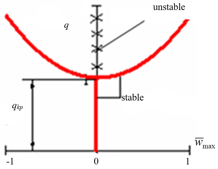
Figure 3. Flat form of equilibrium lamination is unstable, and bending form of lamination is stable.
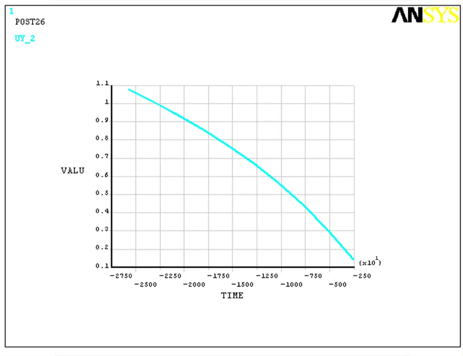
3. Numerical Simulation
When loaded, first, after a loss of stability, the deflection at the center reaches a maximum, corresponding to the main form of equilibrium; then, under heavy loads, a transition to more complex forms is possible. To obtain numerical results, we take data corresponding to the basic form of equilibrium with the subsequent growth of the deflection boom, since this case is more dangerous from the point of view of the growth of the defect. Figure 4 shows the relationship between deflection in the center of the elliptical lamination and the load at different occurrences of the defect $$\overline{h}=0.1;0.08;0.06.$$
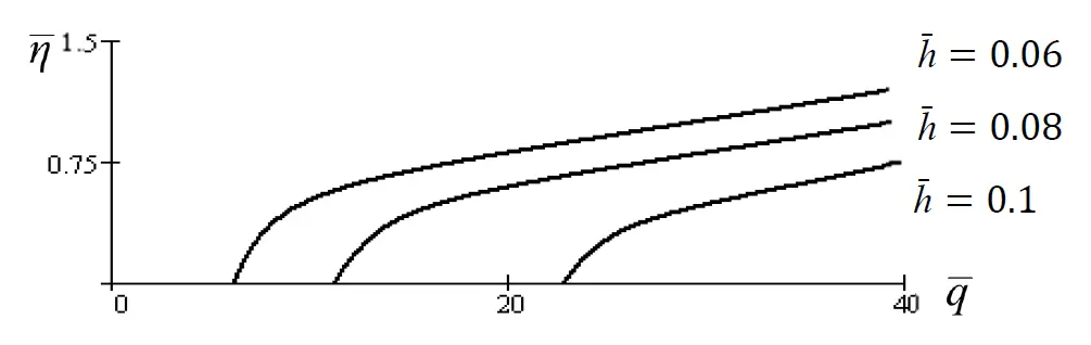
Figure 4. The relationship between deflection in the center of the elliptical lamination and the load at different occurrences of the defect $$\overline{h}=0.1;$$0.08; 0.06.
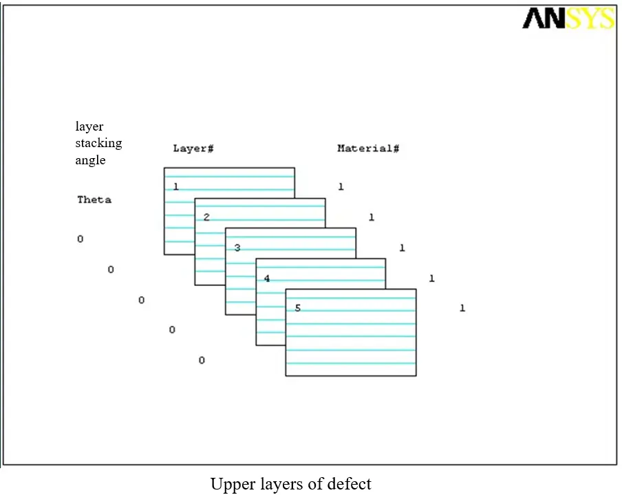
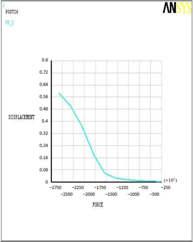
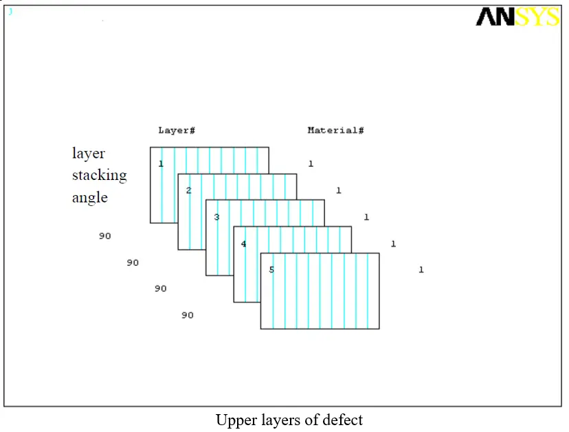
In the work, ANSYS medium [20,21] was used to calculate samples from prepreg (glass fiber), industrial grade of glass fabric—T-25 (VM) TU 6-11-380-76. Unidirectional material has the following characteristics: fiberglass—$${E}_{1}=5.4×1{0}^{4}$$ MPa, $${E}_{2}=1.2×1{0}^{4}$$ MPa, $${G}_{12}=0.5×1{0}^{4}$$ MPa, $$\mu =0.28$$. Figure 5 and Figure 6 show the results of the analysis of the non-linear behavior of elliptical delaminations for the case h = 0.5 mm; Н = 3 mm; а = 15 mm; b = 7 mm; L = 100 mm. The elastic characteristics Ex, Ey, Gxy, $${\mu }_{xy},{\mu }_{yx}$$ of the detached plate are obtained by Equation (1), Equation (2) and Equation (3). The plate consists of 24 layers: the fibers of the exfoliated layer are located in the direction of loading at an angle of 0° (Figure 5); fibers of the peeled layer are located in the direction of loading at an angle of 90° (Figure 6). Arrangement of fibers in direction of loading reduces resistance to deformation (Figure 5), arrangement of fibers in direction perpendicular to loading increases resistance to deformation (Figure 6).
 |
 |
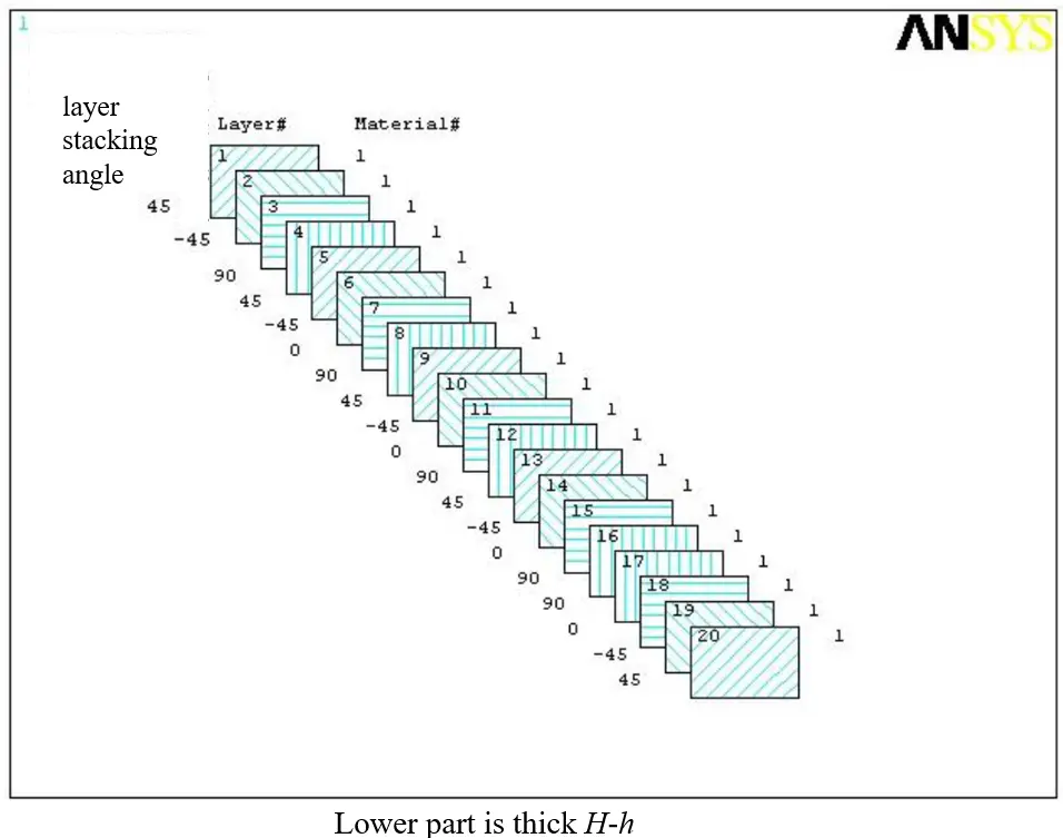 |
Figure 5. Force-strain dependence for laminated part of plate. The fibers of the exfoliated layer are located in the direction of loading at an angle of 0°.
 |
 |
 |
Figure 6. Force-strain dependence for laminated part of plate. The fibers of the exfoliated layer are located in the direction of loading at an angle of 90°.
4. Analysis of the Results of the Calculation
The task of studying the stability of thin-walled laminations of composite materials is considered in a non-linear formulation. A refined approach for solving this class of problems is presented. The problem of stability study in the two-dimensional case is considered using the example of elliptic delaminations in a non-linear formulation. The use of the developed method based on the energy approach allows obtaining explicit analytical expressions for the quantities characterizing the critical load and describing the supercritical behavior of the detached part. The energy method is generalized to the case of analyzing the stability of defects in a non-linear formulation. The value of the critical load was obtained, and the analysis of the supercritical deformation of the defect was made. Forms of equilibrium near the critical point of bifurcation have been investigated. Elastic characteristics of a multilayer package of thin lamination, including the elastic characteristics of separate layers included in it, depending on modulus of elasticity, shear modulus, Poisson’s ratio, and angle of orientation of fibers of unidirectional layer, are determined. Ratios are obtained for the unidirectional composite material, which reflect the contribution of each component (fiber, matrix) in proportion to its volume fraction, the so-called “mixture rule”. The results of the analytical solution are comparable to the numerical data. The strength estimation and numerical calculation methods discussed can also be applied to a wide range of composite materials.
Acknowledgments
The work was carried out within the framework of the grant of the Republic of Belarus for the implementation of the strategic academic leadership program “Priority 2030”.
Author Contributions
Conceptualization, L.B. and S.M.; Methodology, V.R. and A.C.; Software, A.I. and A.N.; Validation, L.B. and V.R.; Formal Analysis, S.M. and A.I.; Investigation, A.C. and A.N.; Resources, S.M.; Data Curation, A.C. and A.I.; Writing—Original Draft Preparation, L.B., V.R. and A.C.; Writing—Review & Editing, L.B., V.R., S.M. and A.C.; Visualization, A.N. and A.I.; Supervision, S.M.; Project Administration, L.B.; Funding Acquisition, Not applicable.
Ethics Statement
Not applicable.
Informed Consent Statement
Not applicable.
Data Availability Statement
Additional data can be provided upon request.
Funding
This research received no external funding.
Declaration of Competing Interest
The authors declare that they have no known competing financial interests or personal relationships that could have appeared to influence the work reported in this paper.Authors Lubov Bokhoeva and Shunqi Mei were employed by Zhejiang Taitan Co., Ltd. The authors declare that this company was not involved in the preparation, writing, and submission of this manuscript.
References
-
Bokhoeva LA, Kurokhtin VY, Chermoshentseva AS, Perevalov AV. Modeling and manufacturing technology of aircraft structures from composite materials. Bull. VSGUTU 2013, 2, 12–18. Available online: https://docs.yandex.ru/docs/view?tm=1770350270&tld=ru&lang=ru&name=VestnikVsgutu2_2013.pdf (accessed on 8 December 2025).
-
Bokhoeva LA, Perevalov AV, Chermoshentseva AS, Kurokhtin VY, Lygdenov BD, Rogov VE. Experimental determination of fatigue resistance characteristics of aviation equipment products. Bull. VSGUTU 2013, 5, 46–53. Available online: https://cyberleninka.ru/article/n/eksperimentalnoe-opredelenie-harakteristik-soprotivleniya-ustalosti-izdeliy-aviatsionnoy-tehniki?ysclid=mlaczwkjic883258646 (accessed on 8 December 2025).
-
Chai H, Babcock CD. Two-dimensional modelling of compressive failure in delami nated laminates. J. Compos. Mater. 1985, 19, 67–98. DOI:10.1177/002199838501900105 [Google Scholar]
-
Chai H, Babcock CD, Knauss WG. One dimensional modelling of failure in laminated plates by delamination buckling. Int. J. Solids Struct. 1981, 17, 1069–1083. DOI:10.1016/0020-7683(81)90014-7 [Google Scholar]
-
Pokrovsky AM, Chermoshentseva AS, Bokhoeva LA. Evaluation of crack resistance of a compressed composite plate with initial delamination. J. Mach. Manuf. Reliab. 2021, 50, 446–454. DOI:10.3103/S1052618821040129. [Google Scholar]
-
Kim J-H. Postbuckling analysis of composite laminates with a delamination. Comput. Struct. 1997, 62, 975–983. DOI:10.1016/S0045-7949(96)00290-8 [Google Scholar]
-
Bokhoeva LA, Baldanov AB. Numerical study of the loss of stability of a polymer composite material. In Proceedings of the VIII International Conference on Problems of Mechanics of Modern Machines, Ulan-Ude, Russia, 4–9 July 2022; pp. 139–142. DOI:10.53980/9785907599055_139 [Google Scholar]
-
Köllner A, Völlmecke C. Post-buckling behaviour and delamination growth characteristics of laminated composite plates. Compos. Struct. 2018, 203, 777–788. DOI:10.1016/j.compstruct.2018.03.010 [Google Scholar]
-
Bokhoeva LA. Study of the stability of plates with defects in a non-linear formulation. News of higher educational institutions. Mech. Eng. 2008, 2, 22–27. Available online: https://cyberleninka.ru/article/n/issledovanie-ustoychivosti-plastin-s-defektami-v-nelineynoy-postanovke-1?ysclid=mladsdnvp9132969227 (accessed on 8 December 2025).
-
Ovesy HR, Kharazi M. Stability analysis of composite plates with through-the-width delamination. J. Eng. Mech. 2011, 137, 87–100. DOI:10.1061/(ASCE)EM.1943-7889.0000205 [Google Scholar]
-
Peck SO, Springer GS. The behavior of delaminations in composite plates analytical and experimental results. J. Compos. Mater. 1991, 25, 907–929. DOI:10.1177/002199839102500708 [Google Scholar]
-
Yin W-L, Jane KC. Refined buckling and postbuckling analysis of two-dimensional delamination—I. Analysis and validation. Int. J. Solids Struct. 1992, 29, 591–610. DOI:10.1016/0020-7683(92)90056-Y [Google Scholar]
-
Bokhoeva LA, Rogov VE, Chermoshentseva AS. Stability of circular defects such as delaminations in structural elements, taking into account transverse shear. Eng. J. Sci. Innov. 2014, 4, 19–22. Available online: https://cyberleninka.ru/article/n/ustoychivost-kruglyh-defektov-tipa-otsloeniy-v-elementah-konstruktsiy-s-uchetom-poperechnogo-sdviga?ysclid=mladv6i442217146499 (accessed on 8 December 2025).
-
Mitrofanov OV. Applied Geometrically Non-Linear Problems in the Design and Calculations of Composite Aircraft Structures; MAI (NIU) Publ.: Moscow, Russia, 2022; 164p. ISBN 978-5-4316-0984-8. [Google Scholar]
-
Alfutov NA, Zinoviev PA, Popov BG. Calculation of Multilayer Plates and Shells Made of Composite Materials; Mashinostroenie: Moscow, Russia, 1984; 264р. [Google Scholar]
-
Kuzmin MA, Lebedev DL, Popov BG. Structural Mechanics and Calculations of Composite Structures for Strength; ICK Akademkniga: Moscow, Russia, 2008; 191р. [Google Scholar]
-
Titov VA, Bokhoeva LA, Baldanov AB. Calculation of Strength Characteristics of Multilayer Composite Materials. Certificate of Registration of the Computer Program RU 2025663286, 27 May 2025; Application No. 2025661391, 12 May 2025. [Google Scholar]
-
Titov VA, Bokhoeva LA, Baldanov AB, Ivanov RP, Bazaron SA. Determination of Stiffness Characteristics of Multilayer Composite Material. Certificate of Registration of the Computer Program RU 2024661132, 15 May 2024; Application No. 2024619405, 26 April 2024. [Google Scholar]
-
Alfutov NA. Fundamentals of Calculation for the Stability of Elastic Systems; Mashinostroenie: Moscow, Russia, 1991; 311р. [Google Scholar]
-
Medvedskiy AL, Martirosov MI, Khomchenko AV. Behavior of layered structural elements made of polymer composite with internal defects under unsteady influences. Mech. Compos. Mater. Struct. 2020, 26, 259–268. DOI:10.33113/mkmk.ras.2020.26.02.259_268.08 [Google Scholar]
-
Urnev AS, Chernyatin AS, Matvienko YG, Razumovsky IA. Experimental and numerical sizing of delamination defects in layered composite materials. Inorg. Mater. 2019, 55, 1516–1522. DOI:10.1134/S0020168519150147 [Google Scholar]