Computer Simulation of the Heat Treatment of Knitting Needles

Computer Simulation of the Heat Treatment of Knitting Needles
Sergei Ivanov 1,2,3,* Mikhail Guryev 2,3,4 Quan Zheng 1,2 Zekui Hu 1,2 Shunqi Mei 1,2 Alexey Guryev 2,3,5
Received: 01 September 2025 Revised: 13 October 2025 Accepted: 28 October 2025 Published: 05 November 2025

© 2025 The authors. This is an open access article under the Creative Commons Attribution 4.0 International License (https://creativecommons.org/licenses/by/4.0/).
1. Introduction
According to the results of studies conducted in [1] on the wear resistance of five samples of knitting machine needles from different manufacturers, the steel used to produce these needles has approximately the same chemical composition, as shown in Table 1.
Statistical analysis of needle failures on knitting machines, presented in the same work, indicates that the failure rates for various reasons are: heel fracture—0.82%, hook fracture—60.27%, latch displacement—8.14%, hook straightening—18.5%, others—11.22%. Fractographic studies of knitting needle fractures conducted by Krasovskii et al. [2] confirm the modeling results carried out in [1] that the transition to the bending of the needle hook is the most stressed and prone to fracture. In addition, all studies [1,2,3,4] establish hook separation as the cause of more than half of knitting needle failures—more precisely, approximately 60%. Therefore, there is reason to consider this type of failure of knitting needles to be one of the priorities, since reducing the likelihood of the hook coming off will at least multiply the service life of knitting needles in general. The authors of [3,4] also came to similar conclusions. In [5], a slightly different approach was applied to solving the problem of hook separation: the authors researched optimizing the design of the knitting needle. The basic premise of the work was that acceleration forces were the main factors contributing to the breakage of hooks. The acceleration value determined in the work was used as input data to analyze the dynamic load on the hook. In the works of Muayad and Habashneh et al. [6,7], it was demonstrated that changing the needle design, if perceived as a beam, can reduce dynamic inertial forces, thereby reducing the risk of fatigue failure. In addition, the data presented in the works of Muayad and Habashneh et al. enable a certain degree of determination of the reliability of knitting needles to some extent, given the necessary data on the properties of the material and the loading conditions of knitting needles. The loading conditions for knitting needles used for calculations can be taken from the works [5,8]. A more uncertain situation arises with the definition of the material and its properties for knitting needles: according to [9], a fairly wide range of steels with a wide variety of properties and characteristics can be used for the manufacture of knitting needles, from ordinary carbon steels with a carbon content of 0.7 wt. % or higher, to corrosion-resistant high-chromium steels such as X10Cr13, X20Cr13, X46Cr13, X65Cr13, X6Cr17, X6CrNi18-10 or X10CrNi18-8.
However, the experimental data presented in [1,10] and based on real studies of the chemical composition of commercial knitting needles indicate that the materials used in this case correspond primarily to supereutectoid steels with an average carbon content of about 1 wt. %. In [10], data on optimal needle heat treatment from the authors’ point of view; this technology involves subjecting the steel to spheroidizing annealing at 680–700 °C, followed by furnace cooling. After that, the steel was heated in a nitrogen atmosphere to temperatures of 780–800 °C (Figure 1) and kept at this temperature for a period of 2 to 16 min (the optimal time, according to the authors of the work, is about 12 min) and then cooled in an oil bath at a temperature of 80 °C. Needles cooled in an oil bath were subjected to tempering operations at temperatures from 250 to 300 °C, while according to the authors of the work, the optimal tempering temperature was 300 °C: despite the fact that there was a slight decrease in hardness (from 700 HV to about 630–650 HV), however, the final indicators of impact strength and fatigue strength The strength showed an increase of 45–50% for impact strength and 20% for fatigue strength, respectively, compared with these parameters in the case of tempering at a temperature of 250 °C.
Conducting field tests to optimize the modes of heat treatment of steels and alloys often associated with significant labor, financial, and time costs. In this case, conducting computer experiments with subsequent analysis and simulating heat treatment modes in a virtual environment can significantly reduce both the time needed to develop and implement a new technology and the cost of experimental research. In addition, in most cases, predictive technical and economic analysis and assessment of the economic effects of introducing the developed technology, compared with the existing one, are possible. A preliminary understanding of the feasibility of conducting final field tests to verify and fine-tune the technological parameters and solutions found by computer modeling methods should eventually result in a decision on their introduction into production.
To carry out a full-fledged cycle of empirical tests on the heat treatment of knitting needles, a considerable amount of equipment is required, including one high-temperature furnace with an operating temperature of up to 1000 °C in a neutral gas atmosphere, as well as one low-temperature furnace with a maximum operating temperature of up to 400 °C, equipped with a device for mixing the atmosphere in the furnace, as well as various devices for quenching and tempering and special baths with quenching media equipped with thermostabilization and mixing devices. In addition, serious laboratory equipment is needed, including various hardness meters and devices for preparing metallographic grinders, as well as a microscope for monitoring the structural and phase states and grain sizes. The approximate cost of one hour of operation of the thermal section is about 500 CNY per hour, excluding the cost of equipment. The operating time of the thermal section during a single experiment is at least 1 h, including heating the thermal furnaces to a preset temperature, installing quenched needles in a special device, and other preparatory actions. The operating time of the laboratory equipment during the analysis of one slot, including preparation, is at least 2 h, with an average cost of about 1000 CNY per hour, not including device costs. Thus, the cost of one empirical experiment will start at 2500 CNY, excluding equipment costs, and will take at least 3 h. In the case of computer simulation, the cost of running a personal computer does not exceed 50 CNY per hour, and the time for one experiment is no more than 10 min, of which about half is spent entering the necessary data into the software package. Thus, at least 4 computer experiments can be conducted in one hour, taking into account the time for technological breaks. That is, the cost of one computer experiment will be about 12.5 CNY, about 200 times less than that of an empirical study.
2. Materials and Methods
The chemical composition shown in Table 2 for sample No. 6 correlates fairly well with the composition of sample No. 4. These samples are likely very similar in chemical composition in terms of carbon and manganese content. However, judging by the photo of the microstructure of this sample, it has a coarser structure of carbide particles, moreover, some of the carbides have an angular shape. This may indicate that spheroidizing annealing was not performed in the case of sample No. 4, or the parameters of this annealing were not optimal for improving the structure of the carbide particles. In addition, to experimentally verify the adequacy of the model, an experiment was conducted on a commercial steel sample with a composition similar to that of Sample No. 6. Thus, taking into account the added data from [10] and the data from the commercial steel sample, Table 1 can be summarized as follows:
Table 2. Chemical composition of steel samples used in simulation.
|
Chemical Composition, Mass. % * |
Sample No. 6 ** |
Sample No. 7 *** |
|---|---|---|
|
C |
1.01 |
1.087 ± 0.008 |
|
Si |
0.24 |
0.267 ± 0.007 |
|
Mn |
0.71 |
0.703 ± 0.003 |
|
P |
0.011 |
0.0104 ± 0.0004 |
|
S |
0.0025 |
0.0021 ± 0.0001 |
|
Cr |
0.409 |
0.398 ± 0.007 |
|
Mo |
0.019 |
0.008 ± 0.001 |
|
Nb |
0.010 |
0.012 ± 0.001 |
* Iron—balance; ** data on this chemical composition are presented in [10], *** commercial steel, chemical composition determined experimentally.
In this work, the simulation of the heat-treatment modes for steel sample No. 6, listed in Table 1, was carried out to optimize the structural and phase state and the required properties, according to the mode stated in [10] as optimal for this steel. In our work, this simulation will be used to further verify the model used to simulate the considered heat treatment parameters in relation to other m odes and steels.
3. Results and Discussion
The applied model is based on Reference [11], and the modeling was performed using a software package from the same study, with its functionality expanded. The most significant points of the functional expansion are presented below:
-
The formulas for calculating the temperatures of critical points Ae1 and Ae3 were replaced by the formulas presented in [12] in order to more accurately account for the influence of the chemical composition of steels and expand the ranges of chemical composition of applicable steels. To calculate the temperature of the critical point Ae1, the new formula looks like this:
(1)
a new formula for calculating the Ae3 critical point:
|
(2) |
where Mn, Si, Cr, Mo, Ni, V, Al, W, S, N, C, Ti, Nb, P, and B are the contents of the corresponding alloying elements in mass %.
Equation (1) and Equation (2) enable a more accurate consideration of the influence of the chemical composition of steel on the position of critical points. The values of the critical points are displayed on the screen as reference information, which is necessary to determine the austenitization temperature.
-
A block of code has been added to predict the maximum possible grain size of austenite depending on the chemical composition and set temperature of austenitization of steel. Formulas for calculating grain size are presented below:
-
-
the natural logarithm of grain size when heated to a temperature in the range (Ac1 < T ≤ Ac3) can be estimated using the formula:
(3)
-
-
the natural logarithm of grain size when heated to a temperature in the range (Ac3< T ≤ Ac3 + 500) is estimated using the following formula:
(4)
where Mn, Si, Cr, Mo, Ni, V, Al, W, S, N, C, Ti, Nb, P, B, Ce are the contents of the corresponding alloying elements in mass %,
$${F}_{1}, { F}_{2}$$ are the grain area, respectively, at the temperature Ac1 and at the austenitization temperature, microns,
T is the heating temperature, °C (for Equation (3))
ΔT is the difference between the current temperature and the Ac3 temperature (for Equation (4)).
Further, the natural logarithm of the resulting grain area can be determined according to the expression:
|
(5) |
Furthermore, knowing the area of the austenitic grain, the diameter of the austenite grain can be determined. The calculation of the grain size of austenite is carried out in this case without taking into account the duration of exposure time, since the knitting needles do not belong to massive parts and, therefore, the time for their complete austenitization is a matter of minutes. In this case, it is natural to omit the effect of exposure time on grain size, since the growth of austenite grains after complete austenitization is predominantly diffusive in nature and, therefore, obeys the laws of diffusion. Accordingly, taking into account the grain size depending on the exposure time makes sense only for long exposures of several tens of minutes or more. In the case of austenitization of knitting needles, their high–temperature exposure time before quenching is usually no more than 10 min (the maximum austenitization time is 16 min according to [10])—during this period, there is no noticeable growth of the austenitic grain.
Predicting the size of an austenitic grain is very important from the point of view of ensuring the ductility and fatigue strength of knitting needle material after quenching: it is a well-known fact that the size of an austenitic grain at the time of quenching inversely correlates with the parameters of plasticity and fatigue strength. That is, the finer the austenite grain is obtained before quenching, the higher the characteristics of ductility, toughness and fatigue strength will be obtained on the finished part after its heat treatment.
To increase the adequacy of the model, it was assumed that the chemical composition of the steels listed in Table 1 of [1] corresponds to that of carbon steels, which contain only carbon, silicon, and manganese as the main alloying elements, and the remaining impurities correspond to the average content of impurities according to the recommendations of the relevant standards. This assumption is made based on the fact that in [1] the content of other alloying elements in the steels under consideration is not given (this, in particular, refers to the content of chromium, nickel, vanadium, molybdenum, and other elements). At the same time, ref. [10] provides a more complete composition of similar steels, which, in addition to the main alloying elements, includes data on the contents of chromium, molybdenum, niobium, sulfur, and phosphorus.
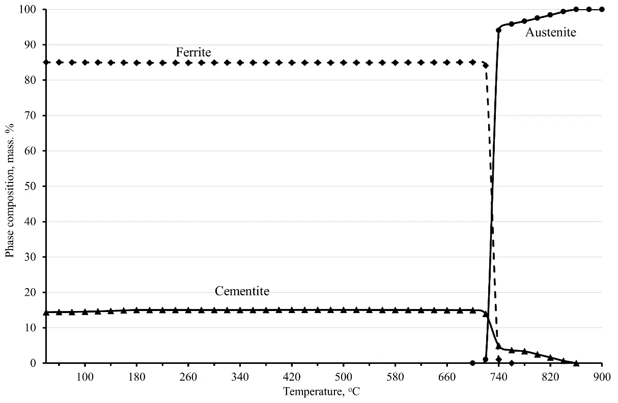
Based on this, it is advisable to construct a phase diagram for steel sample No. 6 over the temperature range from 80 to 900 °C. The phase diagram shown in Figure 1 indicates that there are three main phases in steel within a given temperature range: ferrite, cementite, and austenite.
In the temperature range from 80 to 721 °C, steel is represented by two main phases: ferrite and cementite, which are part of perlite. When heated above 721 °C, a third phase appears—austenite, into which ferrite begins to transform and in which cementite begins to dissolve, the complete transformation of ferrite into austenite in this steel ends at a temperature of 736 °C, and at higher temperatures in the material, there are again only two phases: austenite and cementite.
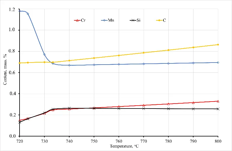
At the same time, regardless of whether there is a further increase in temperature, the cementite dissolution process continues, and a further increase in temperature intensifies the dissolution of cementite. As a result, by the time the sample temperature reaches 800 °C, according to the phase diagram, there is still about 2.3 mass% of cementite left. The rest of the cementite dissolves and enriches the austenite with carbon and alloying elements, in particular chromium. At that time, the carbon concentration in austenite reaches 0.88 wt. % (at the time of the beginning of austenite formation, the carbon concentration in it is about 0.69–0.71 wt. %), and cementite is enriched with chromium, the concentration of which reaches 3.25 wt. % at 800 °C (see Figure 2). Taking into account the fact that before quenching, the steel was previously subjected to spheroidizing annealing, as a result of which the entire cementite acquired a spherical shape with a diameter of spheroids from 0.62 to 0.69 microns, the process of cementite dissolution at the first stage is quite intense.
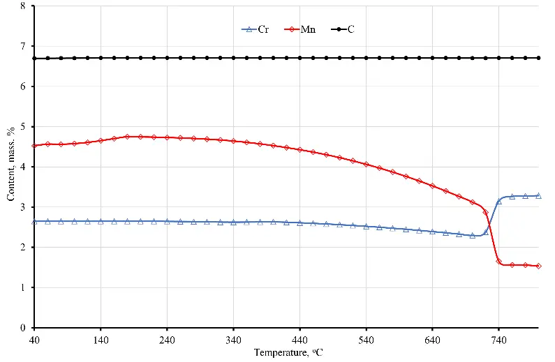
At the same time, chromium enrichment of cementite gradually increases the stability of cementite and the dissolution process begins to slow down. As a result, by the time the hardening is carried out, there are 2.2–2.3 mass % chromium–doped cementite and austenite with a carbon content of about 0.88–0.90 wt. %. During cooling in oil heated to 80 °C, γ→α transformation of austenite occurs, and cementite does not undergo transformations. The average calculated cooling rate in this case was about 4.5–4.6 °C/s, and the formed structural-phase state corresponded to a bainitic-martensitic mixture with distributed carbide inclusions. The data presented in [13,14,15,16] were used to model the temperature dependence of the chemical composition of austenite and cementite.
Figure 3 shows the dynamics of phase transformations occurring during quenching of the material of sample No. 6 from a temperature of 800 °C in oil heated to 80 °C. As can be seen from the diagram in the figure, the final structural-phase state in this case is represented by bainite, martensite and carbide. At the same time, the presence of residual austenite in the amount of about 1.5–1.8 vol. % is also noted. It should be noted that in [10] no mention was made of residual austenite, but its presence was not refuted.
 |
 |
|
(a) |
(b) |
Figure 2. Dependence of the chemical composition of austenite (a) and cementite (b) on the temperature of sample No. 6.
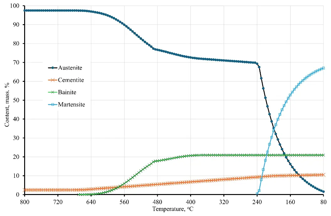
Figure 3. Dynamics of decomposition of supercooled austenite in sample No. 6 upon cooling from a temperature of 800 °C in oil at 80 °C (cooling rate–4.5 °C/s).
Experimental verification of the simulation results of the heat treatment of sample No. 7 was performed on cylindrical samples with a diameter of 1.2 mm and a length of 150 mm. Taking into account the fact that samples No. 6 and No. 7 have a fairly similar chemical composition, computer modeling showed results similar to those for sample No. 6. Experimental verification of the simulation results also demonstrated results similar to the model. During experimental verification, 3 samples of steel No. 7 were rigidly clamped in a special mandrel, which excluded their deformation, and then subjected to heat treatment similar to the recommendations [10]. However, the austenitization temperature was selected based on the results of computer modeling: for example, the austenitization temperature as a result of simulation to find the optimal austenitization temperature It was recommended to reduce it to 792 °C compared to 800 °C for sample No. 6, which was recommended in [10]. As a result, austenitization of sample No. 7 was carried out by placing the mandrel with the samples clamped into it in a preheated furnace filled with nitrogen to a temperature of 790 °C, and the samples were kept in the oven for 14 min, of which 4 min was spent heating the mandrel with samples to the austenitization temperature and 10 min of austenitizing exposure. After the exposure was completed, the samples were removed from the furnace and quenched in oil heated to 80 °C. Then the tempering was carried out in an oven equipped with an air mixing device and heated to 250 °C. The release lasted 60 min, after which the mandrel with the samples was removed from the furnace and cooled in water to room temperature. Upon completion of cooling, the sample mandrel was removed from the water, and then the samples were removed. Two fragments with a length of 5 mm each were cut from each sample. The cutting was performed on a specialized cutting machine, “Microcut–201”. Then, the cut-out samples were placed in a bakelite compound using a METAPRESS metallographic press in such a way that for each initial (out of three) sample, one fragment located along the wire axis (longitudinal sample) and one fragment located across the wire axis (transverse sample) were packed into bakelite. The bakelite-packed samples were sanded and polished using an automatic DIGIPREP grinding and polishing machine. Diamond discs with a grain size of 54, 30, and 15 microns were used as grinding materials. Metallographic grinding was carried out on diamond discs with a grain size of 6 and 3 microns, and then on “MET–Mambo” and “MET–Fox” cloths using diamond suspensions with a grain size of 1 and 0.2 microns. The identification of the phase components of the microstructure was carried out by etching with Berakha’s reagent “3/10” (distinguishing bainite and martensite) and Groesbeck’s reagent (distinguishing carbides and austenite). The phase composition and phase ratio were determined according to the methods [17,18].
The theoretically calculated hardness index for sample No. 6 is 805 HV and for sample No. 7 is 811 HV, which also correlates fairly well (R = 0.98) with the hardness value given in [10]—more than 800 HV after 10 min of austenitization at 800 °C. Graphs of the final hardness of the material of sample No. 6 after tempering are shown in Figure 4. The duration of the tempering was chosen to be 30, 60 and 90 min, and the temperature range was from 200 to 300 °C. As can be seen from the hardness graph, the model used also shows a high level of correlation with the experimental data presented in [10]. A comparison of the simulation and empirical experiment results for sample No. 7 is presented in Table 3.
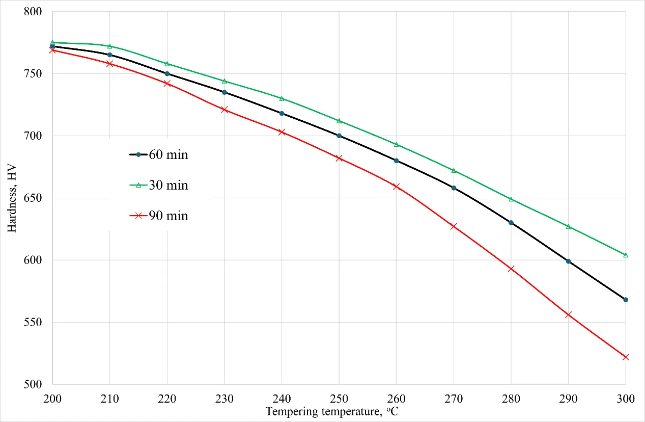
Figure 4. Dependence of the hardness of sample No. 6 after quenching on temperature and tempering time.
Table 3. Comparison of the results of the computer simulation and physical experiment on quenching sample No. 7.
|
Data Indicator |
Simulation Data |
Experimental Data |
Correlation |
|---|---|---|---|
|
Volume fraction of martensite, % |
67.19 |
69.07 ± 0.07 |
0.97 |
|
Volume fraction of bainite, % |
20.91 |
21.35 ± 0.06 |
0.98 |
|
Volume fraction of cementite, % |
10.50 |
8.73 ± 0.08 |
0.80 |
|
Volume fraction of austenite, % |
1.40 |
0.85 ± 0.11 |
0.65 |
|
Hardness after quenching, HV |
811 |
819 ± 4 |
0.99 |
|
Austenite grain diameter, microns |
18.7 |
16.9 ± 0.3 |
0.90 |
|
Hardness after quenching and tempering |
712 |
708 ± 4 |
0.99 |
The Yust model was used to predict hardness after tempering, and the Hollomon–Jaffe parameter was used to estimate temperatures and tempering times beyond the recommended values (T = 390–660 °C and t = 60 min) [13,19]. As shown in Figure 4, the final hardness of steel is affected not only by temperature but also by tempering time. As noted in [10], the optimal vacation parameters are a temperature of 250 °C and a vacation time of 60 min. With these parameters, the hardness of the steel is about 700 HV, however, the sample in this case withstood 25% more cycles of loading without destruction compared to the tempering temperature of 250 °C.
4. Conclusions
As noted in [2], the optimal parameters of tempering are a temperature of 250 °C and a time of 60 min. With these parameters, the hardness of the steel is about 700 HV, however, the sample in this case withstands 25% more cycles of loading without destruction compared to the tempering temperature of 250 °C. The explanation presented in [2] indicates that tempering for 60 min at 300 °C contributes to a more complete release of martensite from dissolved carbon and the formation of finely dispersed isolated inclusions of carbides at the martensite boundaries. However, a tempering temperature of 300 °C leads to a significant decrease in the hardness and strength of steel, which in turn increases the risk of knitting needles failing for other reasons, excluding fatigue. When the tempering time was exceeded by more than 60 min, the authors observed the fusion of carbides and a significant increase in their size, which negatively affected plasticity. At a tempering temperature of 250 °C, a smaller number of finely dispersed inclusions were observed, which suggests that the supersaturation of the martensite crystal lattice with carbon remains; however, in this case, an optimal combination of both strength properties and elastoplastic characteristics was observed. This, in turn, guarantees the greatest service life of knitting needles.
The computer model allows you to calculate the parameters of heat treatment, while key indicators such as hardness and grain diameter show a match with a probability of at least 0.90. At the same time, the model tends to overestimate the grain diameter, whereas in practice this indicator is somewhat smaller. The situation with hardness is not entirely clear: the model tends to slightly decrease hardness after quenching, but the calculated final hardness (after quenching and tempering) exceeds the actual value. However, the hardness values correlate with an accuracy of 0.99, and the discrepancies are mostly attributable to measurement errors. Thus, the computer simulator of heat treatment presented in this paper can generally be used as an alternative to empirical experiments, thereby significantly saving time and resources when optimizing the modes of heat treatment for knitting needles.
Author Contributions
Conceptualization, A.G., S.I., Z.H. and M.G.; Methodology, S.M., S.I. and Q.Z.; Software, S.I.; Validation, S.I., Z.H. and A.G.; Formal Analysis, M.G., Z.H.; Investigation, M.G. and Q.Z.; Resources, S.M.; Data Curation, Q.Z. and S.I.; Writing—Original Draft Preparation, S.I., M.G. and Q.Z.; Writing—Review & Editing, A.G., Q.Z., Z.H. and S.M.; Visualization, S.I. and M.G.; Supervision, S.M. and A.G.; Project Administration, S.M.; Funding Acquisition, Not applicable.
Ethics Statement
Not applicable.
Informed Consent Statement
Not applicable.
Data Availability Statement
Additional data can be provided upon request.
Funding
This research received no external funding.
Declaration of Competing Interest
The authors declare that they have no known competing financial interests or personal relationships that could have appeared to influence the work reported in this paper.
References
- Hu FQ, Zeng XD, Song ZL, Sun PF. An Investigation of the Wear Resistance of Knitting Machinery Needle. Adv. Mater. Res. 2012, 627, 411–416. doi:10.4028/www.scientific.net/amr.627.411. [Google Scholar]
- Krasovskii AY, Kramarenko IV, Gaidamaka VG. Character and causes of in-service needle failure in knitting machines. Strength Mater. 1983, 15, 969–972. doi:10.1007/bf01528942. [Google Scholar]
- Lyon RH, Malinin LM. Needle Fatigue Analysis for High-Speed Knitting Machines. In Proceedings of the ASME 1995 Design Engineering Technical Conferences Collocated with the ASME 1995 15th International Computers in Engineering Conference and the ASME 1995 9th Annual Engineering Database Symposium, Boston, MA, USA, 17–20 September 1995. doi:10.1115/DETC1995-0138. [Google Scholar]
- Chistoborodov GI, Kapralov VV, Nikiforova EN, Onipchenko DA. Prediction of needle failures of basic knitting machines. Technol. Text. Ind. 2014, 2, 127–130. (In Russian) [Google Scholar]
- Kraus H, Speetjens J, Vrrgilio D. Factors Contributing to Hook Failure of Latch Needles in Weft Knitting. Text. Res. J. 1975, 45, 853–863. doi:10.1177/004051757504501204. [Google Scholar]
- Muayad H, Raffaele C, Marco D, Hamed F, Movahedi Rad M. Thermo-mechanical reliability-based topology optimization for imperfect elasto-plastic materials. Int. J. Mech. Mater. Des. 2025, 1–22. doi:10.1007/s10999-025-09799-9. [Google Scholar]
- Habashneh M, Rad MM. Plastic-limit probabilistic structural topology optimization of steel beams. Appl. Math. Model. 2024, 128, 347–369. doi:10.1016/j.apm.2024.01.029. [Google Scholar]
- Zhang W, Liu Y. Wear and fatigue fracture analysis of knitting Needles. Int. J. Sci. 2016, 3, 106–109. [Google Scholar]
- Shvarts Z, Durst FM, Tseller R. Tool for Textiles and Production Method for Same. RU Patent 2682264, 9 December 2014. [Google Scholar]
- Tsuchiya E, Matsumura Y, Hosoya Y, Miyamoto Y, Kobayashi T, Seto K, et al. Development of Niobium Bearing High Carbon Steel Sheet for Knitting Needles. ISIJ Int. 2020, 60, 1052–1062. doi:10.2355/isijinternational.ISIJINT-2019-084. [Google Scholar]
- Collins J, Piemonte M, Taylor M, Fellowes J, Pickering E. A Rapid, Open-Source CCT Predictor for Low Alloy Steels, and Its Application to Compositionally Heterogeneous Material. Metals 2023, 13, 1168. doi:10.3390/met13071168. [Google Scholar]
- Vinokur BB, Pilyushenko VL, Kasatkin OG. The Structure of Structural Alloy Steel; Metallurgiya: Moscow, Russia, 1983; p. 216. (In Russian) [Google Scholar]
- Totten GE. (Ed.) Steel Heat Treatment: Metallurgy and Technologies, 2nd ed.; CRC Press: Boca Raton, FL, USA, 2006; p. 848. doi:10.1201/NOF0849384523. [Google Scholar]
- Guryev AM, Ivanov SG, Garmaeva IA. Diffusion Coatings of Steels and Alloys; scientific and educational center "Management Systems": Barnaul, Russia, 2013; p. 221. (In Russian) [Google Scholar]
- Madeleine DC. Microstructure of Steels and Cast Irons; Springer: Berlin/Heidelberg, Germany; NewYork, NY, USA, 2003; p. 419. doi:10.1007/978-3-662-08729-9. [Google Scholar]
- Brooks CR. Principles of the Heat Treatment of Plain Carbon and Low Alloy Steels; ASM International: Almere, The Netherlands, 1996; p. 490. doi:10.31399/asm.tb.phtpclas.9781627083539. [Google Scholar]
- Ivanov SG, Guryev AM, Zemlyakov SA, Guryev MA, Romanenko VV. Features of the sample preparation methodology for automatic analysis of the carbide phase of steel X12F1 after cementation in vacuum using the software package “Thixomet PRO”. Polzunovskiy Vestn. 2020, 2, 165–168. doi:10.25712/ASTU.2072-8921.2020.02.031. [Google Scholar]
- Ivanov SG, Guryev MA, Guryev AM, Romanenko VV. Phase analysis of boride complex diffusion layers on carbon steels using color etching. Fundam. Probl. Mod. Mater. Sci. 2020, 17, 74–77. doi:10.25712/ASTU.1811-1416.2020.01.012. [Google Scholar]
- Smoljan B, Iljkić D, Totten GE. Mathematical Modeling and Simulation of Hardness of Quenched and Tempered Steel. Metall. Mater. Trans. B 2015, 46, 2666–2673. doi:10.1007/s11663-015-0451-6. [Google Scholar]