Interacting Multiple Model Adaptive Robust Kalman Filter for Position Estimation for Swarm Drones under Hybrid Noise Conditions

Interacting Multiple Model Adaptive Robust Kalman Filter for Position Estimation for Swarm Drones under Hybrid Noise Conditions
Umut Aydemir
1
 Sami Pekdemir
1
Fethi Candan
2,*
Sami Pekdemir
1
Fethi Candan
2,*
Received: 28 August 2025 Revised: 16 September 2025 Accepted: 16 October 2025 Published: 27 October 2025

© 2025 The authors. This is an open access article under the Creative Commons Attribution 4.0 International License (https://creativecommons.org/licenses/by/4.0/).
1. Introduction
The rapid proliferation of Unmanned Aerial Vehicles (UAVs), particularly in swarm configurations, has catalysed transformative advancements across diverse sectors, including surveillance, disaster response, precision agriculture, and defence operations [1,2,3]. The operational efficacy of these multi-agent systems hinges on their ability to perform coordinated manoeuvres, which fundamentally depends on maintaining accurate and robust position estimation [4,5]. However, achieving this is a significant challenge, as swarm operations are frequently compromised by sensor inaccuracies, such as Global Navigation Satellite System (GNSS) multipath errors or signal denial [3,5]; environmental perturbations like wind gusts [5]; and communication latencies inherent to distributed systems [5,6]. These factors can degrade navigational precision, potentially leading to formation collapse or mission failure, especially in dynamic environments where conventional methods falter [5].
The Kalman Filter (KF) has long served as a cornerstone for state estimation in linear systems under the assumption of Gaussian white noise [7,8]. However, this assumption is frequently violated in real-world UAV applications, where noise often exhibits non-Gaussian, heavy-tailed, or non-stationary characteristics, thereby undermining the KF’s optimality [8,9]. Furthermore, the performance of the KF relies on accurate knowledge of the process and measurement noise covariance matrices ($${Q}_{k}$$ and $${R}_{k}$$), which are often unknown or time-varying in practice [10]. To address system non-linearities, extensions such as the Extended Kalman Filter (EKF) [7,11] and sigma-point filters like the Unscented Kalman Filter (UKF) and Cubature Kalman Filter (CKF) have been developed [7,11,12]. While these filters can handle non-linear dynamics, they are not inherently designed to manage complex noise profiles or uncertainties in the noise model [7].
Two primary classes of advanced filters have emerged to enhance performance in challenging environments: robust and adaptive filters [13]. Robust filters are designed to counteract the effects of measurement outliers and heavy-tailed noise [9,14]. This is often achieved by modelling noise with heavy-tailed distributions like the Student’s t-distribution [14] or by employing robust M-estimators based on criteria such as maximum correntropy (MCKF) [15] or centred error entropy (CEEKF) [13,15,16]. These methods typically function by adjusting the measurement noise covariance matrix, $${R}_{k}$$, to down-weight the influence of anomalous measurements [13,16]. In parallel, adaptive filters address process modelling errors and uncertainties that arise from unmodeled target manoeuvres [10]. They operate by introducing a fading factor that inflates the process noise covariance matrix, $${Q}_{k}$$, or the predicted state covariance, $${P}_{k|k-1}$$, thereby increasing the filter’s reliance on new measurements when the dynamic model is deemed unreliable [10].
A critical research gap emerges from these two approaches being strategically opposite [13,14]. Enhancing adaptability to process anomalies involves increasing the Kalman gain, $${K}_{k}$$, to track state changes more aggressively [10]. Conversely, ensuring robustness against measurement outliers requires decreasing the gain to prevent corruption from spurious data [10]. Consequently, a filter optimised for one type of error may perform poorly when confronted with the other, and existing methods often struggle to handle the simultaneous occurrence of both process and measurement modelling errors [13]. While some Adaptive Robust Kalman Filters (ARKF) have been proposed, they often suffer from significant drawbacks; some cannot manage concurrent error types effectively [13], while others introduce considerable time delays through smoothing or post-processing steps, rendering them unsuitable for the real-time demands of UAV navigation [13].
To address these limitations, this paper introduces a novel framework that leverages the Interacting Multiple Model (IMM) algorithm to dynamically and effectively balance these filtering strategies without incurring a time delay. The IMM is a well-established hybrid state estimation technique that probabilistically combines the algorithm outputs [12]. In this approach, the IMM switches between different motion models (e.g., Constant Speed and Constant Turn models for left and right manoeuvres). To rigorously evaluate this framework, a hybrid noise model that combines Gaussian noise with the heavy-tailed Student’s t-distribution is developed to simulate realistic GPS disturbances.
The remainder of this paper is organised as follows: Section 2 details the materials and methods, including the proposed IMM-ARKF framework, the underlying filter models (KF, AKF, and CEEKF), and the simulation setup. Section 3 presents the simulation results, comparing the performance of the proposed IMM-ARKF against existing advanced filters across various noise scenarios. Section 4 discusses the findings, analysing the strengths and trade-offs of the approach. Finally, Section 5 concludes the study and outlines directions for future research.
2. Materials and Methods
2.1. Noise Characterisation
The process noise $${w}_{k-1}$$ adheres to a Gaussian distribution $$N\left(0,Q\right)$$ with covariance $$Q=0.01 {I}_{4}$$, whereas the measurement noise $${v}_{k}$$ deviates from traditional Gaussian modelling to embody non-Gaussian traits more accurately.
In contrast to standard assumptions positing , we formulate via a hybrid distribution engineered to encapsulate the multifaceted nature of drone GPS inaccuracies.
where in conforms to a multivariate Student’s t-distribution characterised by degrees of freedom (dynamically sampled between 25 and 50 to simulate varying heavy-tailed behaviours), a scale parameter , with . The complementary blending factor (tested at 0.1, 0.3, and 0.5) prioritises the Gaussian constituent for routine operations while introducing t-distributed elements to account for sporadic, high-impact outliers. This design choice stems from empirical insights into drone sensor data, where most noise manifests as Gaussian under stable conditions. Yet, intermittent severe deviations, arising from environmental interferences like urban canyons or electromagnetic disruptions, necessitate the heavy-tailed modelling afforded by the Student’s t-distribution. By varying the t-component (10%, 30%, 50%), we evaluate robustness across scenarios, ensuring the model remains computationally tractable without overemphasising rare events. This hybrid perturbation is superimposed on unprocessed GPS readings to mimic authentic sensor anomalies. To enable formation control, subordinate drones derive refined positions relative to the leader via exchanged filtered states over inter-drone channels.
We provide visualisations of its constituent distributions based on numerical simulations to further validate the hybrid noise model’s effectiveness in capturing drone GPS inaccuracies. Figure 1 presents the Gaussian distribution ($$\mu =0, \sigma =1.0$$), which features a symmetric, light-tailed profile suitable for modelling nominal noise under stable flight conditions. Figure 2 displays the Student’s t-distribution with a randomly selected degrees of freedom $$v$$ from the range [25, 50] (e.g., $$v=3$$ in the example) and scale $$\sigma =1.0$$, emphasising its heavier tails that account for rare but significant outliers, such as those from signal multipath or electromagnetic interference. Figure 3 illustrates the hybrid complementary distribution, resulting from a 10% Student’s t and 90% Gaussian blend, which preserves the Gaussian core for typical accuracy while enhancing robustness against extreme deviations. These distributions, derived from 10,000 samples each, reflect the non-stationary and heavy-tailed noise characteristics observed in real-world drone operations. This provides a robust basis for the IMM-ARKF’s performance optimisation.
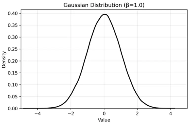
Figure 1. Gaussian Distribution ($$\mu =0, \sigma =1.0$$). The light-tailed profile reflects typical low-variance GPS noise.
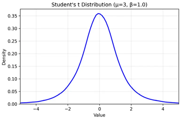
Figure 2. Student’s t-Distribution ($$\mu =0, \sigma =1.0, v=3$$) The heavier tails indicate robustness to outlier events.
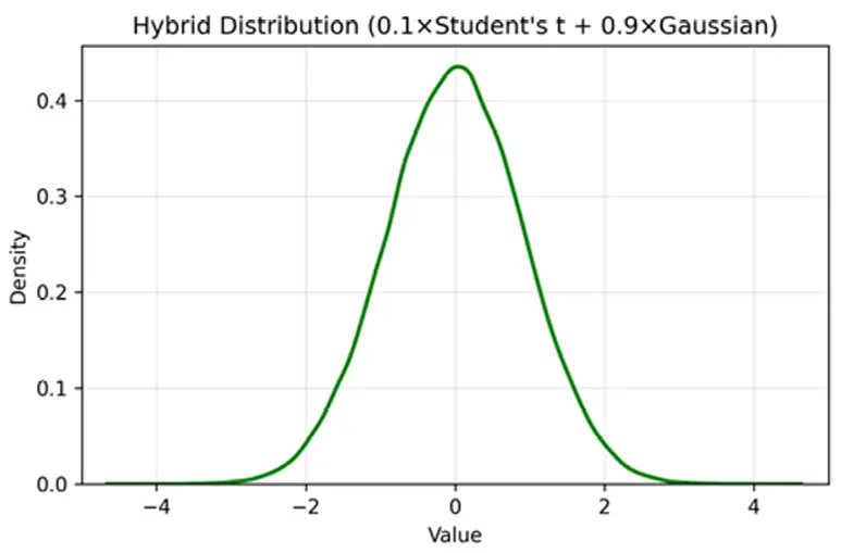
Figure 3. Hybrid Complementary Noise Model (10% Student’s t + 90% Gaussian). This blended distribution balances nominal and outlier-prone noise characteristics.
2.2. Interacting Multiple Model
The IMM approach is a widely recognised technique for state estimation in dynamic systems with multiple operating modes, such as manoeuvring and non-manoeuvring states. It effectively handles model uncertainties by integrating multiple models, making it particularly suitable for applications like unmanned aerial vehicle (UAV) localisation where motion patterns can vary. The IMM fusion process combines estimates from three models: one constant velocity model ($${F}_{C{V}_{M}}$$) and two constant turning models ($${F}_{C{T}_{M}}$$) for left and right manoeuvres. The transition matrices are defined as follows:
where $$∆t$$ is the sampling time, and $${\omega }_{i}$$ is the turn rate, set to $$\omega =\frac{2\pi }{180}$$ for the left turn and $$\omega =-\frac{2\pi }{180}$$ for the right turn. The IMM fusion process integrates the outputs from the three-transition model through a cyclical procedure that probabilistically combines their estimates, enabling the filter to seamlessly adapt to varying error sources in swarm drone operations. The cycle commences with the mixing phase, where predicted mode probabilities are calculated to forecast the likelihood of each model at the current timestep based on prior probabilities and transitions:
These predictions reflect the expected evolution of model relevance, incorporating the transition matrix’s bias toward mode persistence while permitting shifts when evidence warrants.
The Markov transition matrix is
The initial model probability of the three-transition model is set to
Next, mixing weights are derived to blend the posterior estimates from the previous timestep, creating conditioned priors for each model:
ensuring that the input to sub-model $$j$$ is a weighted average informed by how likely transitions from other models are. The mixed state and covariance for each $$j$$ are then:
This mixing incorporates cross-model information, enhancing overall robustness by propagating uncertainty across modes.
The mode probability update phase evaluates how well each model matches the current observation via Gaussian likelihoods, assuming the innovation is zero-mean under the correct model:
where $$m=2$$ is the measurement dimension. These likelihoods, which quantify model-data agreement, are used to refine probabilities:
Finally, the combination phase fuses the mode-conditioned estimates into a single output, weighted by updated probabilities:
This probabilistic fusion yields a multimodal estimate that captures uncertainty across models, providing a comprehensive state representation resilient to mixed errors in drone swarms.
2.3. The Proposed Adaptive Robust Kalman Filter (ARKF)
The Adaptive Robust Kalman Filter (ARKF) is specifically engineered to handle process modelling errors and measurement outliers commonly occurring in drone swarm operations. Unlike conventional Kalman filters that assume Gaussian noise distributions, the ARKF incorporates robust estimation techniques and adaptive mechanisms to maintain accurate state estimation under adverse conditions such as sudden wind disturbances, GPS signal interference, and sensor malfunctions.
The ARKF begins with standard Kalman filter prediction equations:
The innovation (residual) and its covariance are computed as:
The ARKF employs a robust weight function based on the Gaussian kernel to handle measurement outliers. The whitened residual is first computed using the square root of the measurement noise covariance:
where contains the eigenvectors and contrains eigenvalues of .
The whitened observation and measurement matrix are:
The whitened residual becomes:
The robust weight functions are constructed using Gaussian kernels with two different bandwidth parameters. The first weight matrix accounts for individual measurement reliability:
The second weight matrix captures the relationships between different measurement components:
The combined robust weight matrix is:
where $$h\in \left[0, 1\right]$$ is a mixing parameter that balances individual and cross-component robustness.
The updated measurement noise covariance becomes:
To detect and compensate for process modelling errors, the ARKF incorporates an adaptive scaling factor . The scaled prediction covariance and innovation covariance are:
The Mahalanobis distance is computed to detect process anomalies:
If ( for % 95% confidence with m = 2 degrees of freedom), the adaptive factor is updated iteratively:
2.4. Simulation Setup and Environment
To evaluate the efficacy of the proposed IMM-ARKF framework for position estimation and formation control in swarm drones, simulations were conducted within the Webots robotics simulator (Version 2025a), a versatile open-source platform renowned for its realistic physics engine and support for multi-agent systems. The simulation environment replicates a controlled outdoor scenario, encompassing a flat terrain with a flight area sufficient for a single, distinct trajectory. This trajectory consists of a figure-8 pattern composed of two circles, each with a 20 m radius. This specific trajectory was chosen to test the framework’s performance and adaptability to a challenging, non-linear motion profile.
The drone models are based on the Crazyflie 2.0 quadrotor, a lightweight (27 g) nano-drone known for its agility and suitability for swarm applications due to its compact size (92 mm diagonal) and onboard sensors including IMU, GPS, and gyroscopes. The equipment was sourced from Bitcraze AB, located in Malmö, Sweden. In Webots, each drone is instantiated using a customised prototype that integrates four brushless motors, a camera for potential visual feedback (though not utilised here for GPS-focused estimation), and communication emitters/receivers for inter-drone data exchange. A swarm of 9 drones was deployed: one leader drone navigating the predefined square trajectory, and eight follower drones maintaining relative positions. The formation configuration adopts a linear chain topology, where each follower tracks the preceding drone at a desired separation of 0.5 m, ensuring collision avoidance and cohesion. Figure 4 illustrates the Webots environment utilized for the evaluation. The Webots robotic simulator (Version 2025a) was selected as the open-source platform due to its realistic physics engine and its support for multi-agent systems. Complementing this, Figure 5 depicts the initial alignment of nine Crazyflie 2.0-based unmanned aerial vehicles (UAVs). This figure specifically confirms the implementation of the linear chain topology, where the leader is positioned at the front and the eight followers are placed at precise intervals.


Figure 5. Swarm Formation Initialisation. Nine Crazyflie 2.0-based drones aligned in a chain, with the leader positioned ahead.
Control mechanisms are implemented via a PID velocity-fixed-height controller [18], which regulates forward, sideways, and yaw velocities while maintaining a constant altitude of 1.0 m. The PID parameters were tuned empirically: proportional gains of 0.05 for velocity components (forward/sideways), 1.0 for yaw, and 0.5 for roll/pitch attitude, with derivative gains of 0.05 (velocity and roll/pitch) and 0.5 (yaw), and altitude-specific gains of 10.0 (proportional), 5.0 (integral), and 5.0 (derivative) to minimise overshoot and steady-state errors. This controller processes filtered position estimates from the IMM-ARKF, computing motor velocities for the four rotors (with alternating signs for torque balance) to achieve maximum speeds of 0.4 m/s.
The simulation incorporates the hybrid noise model detailed in Section 2.1, applied exclusively to follower drones GPS measurements to simulate realistic sensor degradation. Performance logging captures true, noisy, and filtered position histories for RMSE computation, with the leader operating noise-free for baseline comparison. Figure 6 depicts a dynamic snapshot of the swarm mid-simulation, showing trajectory adherence under noise, with overlaid error ellipses representing IMM-ARKF covariance estimates. This setup not only validates the filter’s robustness but also demonstrates practical scalability for larger swarms in applications like aerial surveying or coordinated search operations.
Simulations were conducted using a high-fidelity robotics simulator to evaluate the efficacy of the proposed IMM-ARKF for position estimation and trajectory tracking in UAV swarms. The setup involved a swarm comprising a leader UAV and multiple follower UAVs, where the leader executed a predefined trajectory, and the followers maintained formation through relative position estimation under noisy measurements. The IMM-ARKF was implemented to fuse multiple filtering models, addressing uncertainties arising from non-Gaussian noise sources prevalent in real-world UAV operations, such as sensor inaccuracies and environmental disturbances.
The initial conditions for the IMM-ARKF were configured as follows. The state vector was initialised as , representing the 2D position and velocity components in the inertial frame. The initial covariance matrix was set to , assuming uniform uncertainty across states. The state transition matrix incorporated a constant velocity model with sampling interval s.

Figure 6. Mid-Simulation Snapshot of Drone Trajectories. Illustrates formation maintenance under hybrid noise, with filtered paths and covariance ellipses.
The mode transition probability matrix $$\mathrm{\Pi }$$ for the interacting multiple model framework was defined as
with initial mode probabilities $${\mu }_{0}=\left[\begin{array}{ccc}0.4& 0.3& 0.3\end{array}\right]$$ distributed according to IMM-ARKF. Adaptive parameters for robustness included the correntropy weighting factor $$h=0.15$$, and kernel bandwidths $${\sigma }_{1}=2$$ and $${\sigma }_{2}=8$$.
To simulate realistic UAV sensor degradations, GPS measurements were corrupted with the hybrid noise model described in Section 2.1, using mixtures of Gaussian and Student’s t-distributions in ratios of 10%, 30%, and 50% Student’s t. These conditions, visualised in Figure 1, Figure 2 and Figure 3, reflect increasing outlier influence, enabling robust evaluation of the IMM-ARKF’s performance. Figure 7 illustrates the probability density functions of these composite noise distributions, highlighting the increasing influence of heavy tailed outliers as the Student’s t-distribution proportion rises.
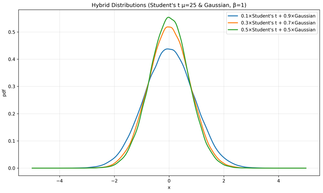
Table 1 presents the initial parameter values for the IMM filters (IMM-ARKF, IMM-KF, IMM-EKF). These values were selected empirically and define the baseline configuration for the comparative analysis, ensuring that all three filters operate within the same Interacting Multiple Model (IMM) framework.
Table 1. Initial Parameter Settings for IMM Filters.
|
Parameter |
IMM-ARKF |
IMM-KF |
IMM-EKF |
|---|---|---|---|
|
Initial Mode Probabilities |
|
|
|
|
Mode Transition Matrix |
|
|
|
|
Initial State |
|
|
|
|
Initial Covariance |
|
|
|
|
Process Noise Covariance |
|
|
|
|
Measurement Noise Covariance |
(Dynamic: 0.5, 1.5, 8) |
(Dynamic: 0.5, 1.5, 8) |
(Dynamic: 0.5, 1.5, 8) |
|
Measurement Matrix |
|
|
Dynamic Jacobian |
|
State Transition Matrix |
CV, CT+, CT−
|
CV, CT+, CT−
|
CV, CT+, CT−
|
|
Model-Specific Parameters |
, , |
None (Nominal Gaussian) |
None (Nonlinear Jacobian) |
3. Results
The performance of the proposed IMM-ARKF, IMM-EKF, and IMM-KF was evaluated for a leader-follower swarm of nine drones in the Webots simulation environment. 100 Monte Carlo simulations were conducted to assess the robustness and accuracy of these filters under hybrid noise conditions combining Gaussian and Student’s t-distributions at proportions of 10%, 30%, and 50%.
Figure 8 presents bar charts that depict the RMSE performance of each filter for different noise covariances ($$R = 0.5I, 1.0I, 8.0I$$). This figure emphasises the temporal robustness of the filters as noise conditions evolve.
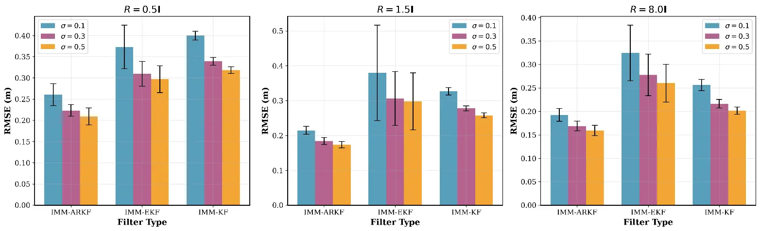
Figure 9 displays bar charts comparing the average execution times of the filters across the same noise standard deviations. This figure underscores the computational trade-offs associated with each filtering approach, providing a clear view of their efficiency.
The numerical results from these simulations are summarised in Table 2, which compiles the mean and standard deviation of RMSE and average execution times for each filter across the tested noise scenarios, offering a comprehensive quantitative assessment.
Table 2. RMSE Performance Comparison Across Different Noise Covariances.
|
Filter Type |
Student’s t Noise Ratio |
RMSE ($$\bm{R}=0.5{\bm{I}}_{2}$$) |
RMSE ($$\bm{R}=1.5{\bm{I}}_{2}$$) |
RMSE ($$\bm{R}=8{\bm{I}}_{2}$$) |
Avg. Time (ms) |
||||
|---|---|---|---|---|---|---|---|---|---|
|
Mean |
Std |
Mean |
Std |
Mean |
Std |
Mean |
Std |
||
|
IMM-ARKF |
10% |
0.2602 |
0.026 |
0.2121 |
0.0114 |
0.1925 |
0.0138 |
1.7087 |
0.0717 |
|
30% |
0.2232 |
0.0137 |
0.1825 |
0.01 |
0.1709 |
0.0104 |
1.6378 |
0.129 |
|
|
50% |
0.2066 |
0.0198 |
0.1765 |
0.0091 |
0.1579 |
0.0114 |
1.6402 |
0.0975 |
|
|
IMM-EKF |
10% |
0.3763 |
0.0512 |
0.3781 |
0.1361 |
0.3224 |
0.0596 |
0.6297 |
0.056 |
|
30% |
0.3115 |
0.0293 |
0.3046 |
0.0778 |
0.2781 |
0.0446 |
0.6712 |
0.0764 |
|
|
50% |
0.2933 |
0.0314 |
0.3012 |
0.0813 |
0.2597 |
0.0398 |
0.689 |
0.0986 |
|
|
IMM-KF |
10% |
0.3937 |
0.0105 |
0.3255 |
0.0106 |
0.2528 |
0.0119 |
0.9436 |
0.0683 |
|
30% |
0.3394 |
0.0093 |
0.2778 |
0.074 |
0.2168 |
0.009 |
0.8472 |
0.0572 |
|
|
50% |
0.3199 |
0.0077 |
0.2555 |
0.07 |
0.1995 |
0.0079 |
0.8991 |
0.0673 |
|
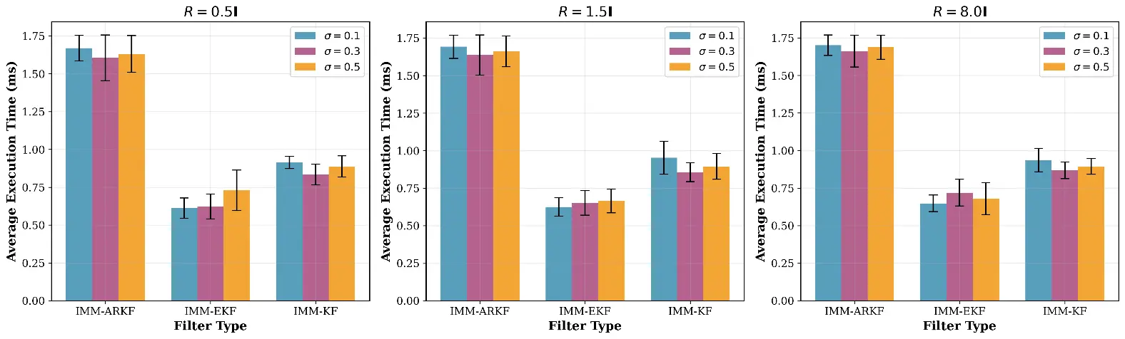
Figure 10 shows the filtered trajectories of UAVs 2, 4, 6, and 8 in the leader-follower swarm and compares the performance of IMM-ARKF, IMM-KF, and IMM-EKF under hybrid noise conditions. The IMM-ARKF trajectories (red dashed lines) closely follow the actual trajectories, demonstrating accuracy and formation stability, while IMM-KF (green dashed lines) and IMM-EKF (blue dashed lines) show larger deviations, especially in the high-curvature sections of the figure-of-8 trajectory.

Figure 10. Combined Trajectory Comparison for Drones 2, 4, 6, and 8 Across IMM-ARKF, IMM-KF, and IMM-EKF Filters.
The presented results offer a compelling narrative about the practical advantages of the proposed IMM-ARKF framework. The quantitative data, summarised in Table 2, clearly establishes a performance hierarchy: the IMM-ARKF consistently yields the lowest Root Mean Square Error (RMSE) across all tested noise profiles. This superiority is not marginal; it becomes increasingly pronounced as the proportion of heavy-tailed Student’s t-distributed noise grows, which simulates more challenging real-world conditions. This trend indicates that while standard filters like IMM-KF and IMM-EKF perform adequately under nominal Gaussian noise, their accuracy degrades significantly in the presence of measurement outliers. In contrast, the IMM-ARKF demonstrates exceptional resilience, a direct consequence of its robust filtering component. The trade-off, however, is evident in the execution time analysis (Figure 9), which confirms that the enhanced accuracy of the IMM-ARKF comes at the cost of increased computational complexity due to its more sophisticated adaptive and iterative processes.
Beyond the numerical metrics, the trajectory plots in Figure 10 provide a powerful visual confirmation of the filter’s effectiveness. The path estimated by the IMM-ARKF closely mirrors the true figure-8 trajectory, maintaining formation stability even in the high-curvature turns where manoeuvring challenges are greatest. Conversely, the trajectories from the IMM-KF and IMM-EKF exhibit noticeable deviations and oscillations, suggesting they are more susceptible to being “pushed off course” by the sporadic, high-magnitude errors characteristic of the hybrid noise model. This visual evidence underscores that the IMM-ARKF does not merely achieve a better statistical average; it produces a more stable and reliable flight path, which is critical for collision avoidance and mission success in swarm operations.
Finally, the success of the overall approach is rooted in the intelligent synthesis of two distinct strategies, managed by the Interacting Multiple Model (IMM) framework. The system’s ability to probabilistically switch between the Constant Velocity (CV) and Constant Turn (CT) models allows it to accurately represent the drone’s manoeuvring dynamics without resorting to a more complex and computationally expensive full dynamic model. Simultaneously, the adaptive and robust mechanisms within the ARKF address the opposing challenges of process and measurement errors. As highlighted in the literature, adaptability (handling model uncertainty) and robustness (rejecting measurement outliers) are conflicting goals, as one typically requires increasing the filter gain while the other requires decreasing it. The IMM-ARKF architecture elegantly resolves this conflict by probabilistically blending filter outputs, ensuring that the final state estimate is both dynamically adaptive and robust to sensor noise. The results, therefore, do not just show the superiority of a single filter but validate the effectiveness of a hybrid architectural choice that balances these competing requirements in real-time.
4. Discussion
The simulation results from this study strongly validate the superior performance of the proposed Interacting Multiple Model Adaptive Robust Kalman Filter (IMM-ARKF) for the position estimation of swarm drones operating under hybrid noise conditions. When tested against noise profiles that combine Gaussian and heavy-tailed Student’s t-distributions, the IMM-ARKF consistently demonstrated significant improvements in accuracy, achieving a root mean square error (RMSE) reduction of up to 43.9% compared to the Interacting Multiple Model Extended Kalman Filter (IMM-EKF) and up to 34.9% compared to the Interacting Multiple Model Kalman Filter (IMM-KF). This performance enhancement was particularly evident in scenarios with a higher proportion of Student’s t-distributed noise, underscoring the IMM-ARKF’s robustness in managing the heavy-tailed outliers that simulate real-world challenges such as GPS signal jamming or multipath effects in urban environments.
The core strength of our proposed model lies in its strategic fusion of adaptive and robust filtering mechanisms within the IMM framework, a concept supported by state-of-the-art research [3]. Our approach effectively addresses the simultaneous presence of both process modelling errors and measurement outliers, a common yet challenging issue in UAV navigation [3]. Recent work by Yang et al. (2024) proposed a similar IMMARKF that combines a standard Kalman Filter (KF), an Adaptive Kalman Filter (AKF) for process anomalies, and a robust Centred Error Entropy Kalman Filter (CEEKF) for measurement outliers [3]. Their findings corroborate ours, confirming that such hybrid approaches can better adapt to non-stationary noise and environments where both types of anomalies occur concurrently [3]. This is a notable advantage over methods that employ either a singular adaptive or a singular robust filter, as the strategies for handling these two error types are fundamentally opposite: adaptability requires increasing the filter gain, whereas robustness necessitates decreasing it. Other contemporary research has also explored robust IMM filters for UAVs, such as the IMM-Maximum Correntropy Kalman Filter (IMM-MCKF) for environments with Student’s t-distributed noise [6] and the robust cubature Kalman filter-based IMM (IMM-RCKF) [13]. Our findings are consistent with this body of work, which collectively shows that robust IMM filters significantly outperform standard counterparts in non-Gaussian conditions, albeit often at an increased computational cost.
A key design choice in our study was the use of kinematic motion models, specifically, Constant Velocity (CV) and Constant Turn (CT) within the transition matrix, instead of more complex dynamic models. This decision was made to reduce model complexity and computational overhead, a strategy validated by Lizzio et al. (2023) [19]. Their research compared CV, CT, and a full-state (FS) dynamic model for UAV swarm target estimation, concluding that an IMM framework with simpler kinematic models can effectively track manoeuvring targets without the high computational load or the need for prior knowledge of the target’s physical parameters, which is often required by full dynamic models [19]. Our results support this conclusion, demonstrating that the probabilistic switching of the IMM effectively compensates for the simplicity of the individual motion models.
Furthermore, a simple Proportional-Integral-Derivative (PID) controller was intentionally employed for formation control. While more advanced controllers, such as Model Predictive Control (MPC), could potentially yield better tracking performance [20], our objective was to isolate and demonstrate the efficacy of the estimation algorithm itself. We highlight the robustness and accuracy of the IMM-ARKF’s state estimates by achieving stable formation control with a basic controller. The use of a simple controller ensures that the observed performance improvements are directly attributable to the quality of the state estimation rather than the sophistication of the control law.
Despite the strong performance, certain limitations should be acknowledged. The Webots simulation, while realistic, may not fully capture all real-world complexities like dynamic wind gusts or specific hardware-induced noise patterns. Moreover, the IMM framework’s reliance on a fixed set of motion models could be a constraint in scenarios involving highly erratic or unpredictable swarm manoeuvres. A significant limitation inherent in many IMM applications is the use of a fixed and predefined Transition Probability Matrix (TPM) [16]. As shown by Cosme et al. (2021), an inaccurate or non-optimal TPM can degrade estimation performance, especially if the target’s manoeuvring behavior changes over time [16]. Therefore, a promising direction for future work is integrating an adaptive TPM estimation mechanism, which could further enhance the filter’s robustness to unforeseen target manoeuvres [16].
5. Conclusions
This study proposed and validated an Interacting Multiple Model Adaptive Robust Kalman Filter (IMM-ARKF) as a highly effective solution for the position estimation of swarm drones operating in environments compromised by hybrid non-Gaussian noise. By systematically evaluating its performance against standard IMM-KF and IMM-EKF approaches, this work demonstrates that the IMM-ARKF substantially improves navigational accuracy. The proposed filter achieved significant RMSE reductions, up to 43.9%, particularly in scenarios with heavy-tailed measurement noise, which are representative of real-world operational challenges like GNSS signal degradation.
The superiority of the IMM-ARKF stems from its novel architecture, which synergistically fuses an adaptive filter to account for process model uncertainties with a robust filter designed to mitigate the impact of measurement outliers. This dual capability is managed dynamically by the model probability mechanism of the IMM framework, allowing the system to adapt in real-time to varying error characteristics without the time delays associated with other advanced methods. This adaptability enhances the reliability and safety of multi-UAV operations in environments where clean sensor data and perfect models are unattainable, such as in urban canyons or during signal denial.
While the enhanced accuracy is achieved at the cost of moderately increased computational time, the trade-off is justified for applications where navigational integrity is paramount. The findings confirm that a well-designed estimator can ensure robust performance even with simplified kinematic models and basic controllers, thereby highlighting the central role of state estimation in autonomous systems.
Future work will focus on validating these findings through hardware-in-the-loop experiments and real-world flight tests to account for additional environmental dynamics. Further research could also explore the integration of an adaptive transition probability matrix to enhance robustness against unpredictable manoeuvres and the optimisation of the algorithm for deployment on resource-constrained onboard processors. Ultimately, the IMM-ARKF framework represents a significant step toward enabling safe, reliable, and scalable autonomous operations for UAV swarms in complex and unpredictable environments.
Statement of the Use of Generative Al and Al-Assisted Technologies in the Writing Process
During the preparation of this manuscript, author U.A. used Gemini (Google) in order to improve the grammar, clarity, and readability of the text. After using this tool/service, the authors reviewed and edited the content as needed and takes full responsibility for the content of the published article.
Author Contributions
Conceptualization, F.C. and U.A.; Methodology, F.C. and U.A.; Software, U.A.; Validation, F.C., U.A. and S.P.; Formal Analysis, U.A.; Investigation, U.A.; Visualization, U.A.; Writing—Original Draft Preparation, U.A.; Writing—Review & Editing, F.C., U.A. and S.P.; Supervision, F.C.
Ethics Statement
Not applicable.
Informed Consent Statement
Not applicable.
Data Availability Statement
No datasets were used or analyzed in this study.
Funding
This research received no external funding.
Declaration of Competing Interest
The authors declare that they have no known competing financial interests or personal relationships that could have appeared to influence the work reported in this paper.
References
-
Chen M, Xiong Z, Xiong J, Wang R. A hybrid cooperative navigation method for UAV swarm based on factor graph and Kalman filter. Int. J. Distrib. Sens. Netw. 2022, 18, 155014772110647. doi:10.1177/15501477211064758. [Google Scholar]
-
Zhao L, Chen B, Hu F. Research on swarm control based on complementary collaboration of unmanned aerial vehicle swarms under complex conditions. Drones 2025, 9, 119. doi:10.3390/drones9020119. [Google Scholar]
-
Yang B, Wang H, Shi Z. Interacting multiple model adaptive robust Kalman filter for process and measurement modeling errors simultaneously. Signal Process. 2024, 227, 109743. doi:10.1016/j.sigpro.2024.109743. [Google Scholar]
-
Gadsden SA, Wilkerson S, Alshabi M. Fault Detection of a Mechatronic System Using Interacting Operating Modes. In Proceedings of the Canadian Society for Mechanical Engineering International Congress, Charlottetown, PE, Canada, 27–30 June 2021; Volume 3. doi:10.32393/csme.2021.202. [Google Scholar]
-
Radhika MN, Mallick M, Tian X. IMM Filtering Algorithms for a highly maneuvering fighter aircraft: An overview. Algorithms 2024, 17, 399. doi:10.3390/a17090399. [Google Scholar]
-
Candan F, Beke A, Shen C, Mihaylova L. An Interacting Multiple Model Correntropy Kalman Filter Approach for Unmanned Aerial Vehicle Localisation. In Proceedings of the 2021 International Conference on INnovations in Intelligent SysTems and Applications (INISTA), Kocaeli, Turkey, 25–27 August 2021; pp. 1–6. doi:10.1109/inista55318.2022.9894214. [Google Scholar]
-
Rodríguez AJ, Sanjurjo E, Pastorino R, Naya MÁ. Multibody-Based input and state observers using adaptive extended Kalman filter. Sensors 2021, 21, 5241. doi:10.3390/s21155241. [Google Scholar]
-
Al-Absi MA, Fu R, Kim K-H, Lee YS, Al-Absi AA, Lee H-J. Tracking unmanned aerial vehicles based on the Kalman filter considering uncertainty and error aware. Electronics 2021, 10, 3067. doi:10.3390/electronics10243067. [Google Scholar]
-
Huai L, Li B, Yun P, Song C, Wang J. Weighted Maximum Correntropy Criterion-Based Interacting Multiple-Model filter for maneuvering target tracking. Remote Sens. 2023, 15, 4513. doi:10.3390/rs15184513. [Google Scholar]
-
Zhang J, Zhou W, Wang X. UAV swarm navigation using dynamic adaptive Kalman filter and network navigation. Sensors 2021, 21, 5374. doi:10.3390/s21165374. [Google Scholar]
-
Zhang L, Sidoti D, Bienkowski A, Pattipati KR, Bar-Shalom Y, Kleinman DL. On the Identification of Noise Covariances and Adaptive Kalman Filtering: A New Look at a 50 Year-Old Problem. IEEE Access 2020, 8, 59362–59388. doi:10.1109/access.2020.2982407. [Google Scholar]
-
Hematulin W, Kamsing P, Torteeka P, Somjit T, Phisannupawong T, Jarawan T. Trajectory planning for multiple UAVs and hierarchical collision avoidance based on nonlinear Kalman filters. Drones 2023, 7, 142. doi:10.3390/drones7020142. [Google Scholar]
-
Liu X, Liu X, Zhang W, Yang Y. Interacting multiple model UAV navigation algorithm based on a robust Cubature Kalman filter. IEEE Access 2020, 8, 81034–81044. doi:10.1109/access.2020.2991032. [Google Scholar]
-
Lee AS, Wu Y, Gadsden SA, AlShabi M. Interacting multiple model estimators for fault detection in a magnetorheological damper. Sensors 2023, 24, 251. doi:10.3390/s24010251. [Google Scholar]
-
Zhao F, Cai R. Adaptive particle filter for state estimation with application to non-linear system. IET Signal Process. 2022, 16, 1023–1033. doi:10.1049/sil2.12147. [Google Scholar]
-
Cosme LB, D’Angelo MFSV, Caminhas WM, Camargos MO, Palhares RM. An adaptive approach for estimation of transition probability matrix in the interacting multiple model filter. J. Intell. Fuzzy Syst. 2021, 41, 155–166. doi:10.3233/jifs-201129. [Google Scholar]
-
Cyberbotics. Webots Main Window. Available online: https://cyberbotics.com/#cyberbotics (accessed on 23 September 2025). [Google Scholar]
-
Bitcraze. pid_controller.py. GitHub Repository. Available online: https://github.com/bitcraze/crazyflie-simulation/blob/main/controllers_shared/python_based/pid_controller.py (accessed on 23 September 2025). [Google Scholar]
-
Lizzio FF, Bugaj M, Rostáš J, Primatesta S. Comparison of multiple models in decentralized target estimation by a UAV swarm. Drones 2023, 8, 5. doi:10.3390/drones8010005. [Google Scholar]
-
Huang H, Zhou H, Zheng M, Xu C, Zhang X, Xiong W. Cooperative Collision Avoidance Method for Multi-UAV Based on Kalman Filter and Model Predictive Control. In Proceedings of the 2019 IEEE International Conference on Unmanned Systems and Artificial Intelligence (ICUSAI), Xi’an, China, 22–24 November 2019; pp. 1–7. doi:10.1109/icusai47366.2019.9124863. [Google Scholar]