Guidance and Control System for an Unmanned Combat Aerial Vehicle as a Wingman

Guidance and Control System for an Unmanned Combat Aerial Vehicle as a Wingman
Faisal A. Alhosani 1,2,* James F. Whidborne 2
Received: 30 July 2025 Revised: 01 September 2025 Accepted: 22 September 2025 Published: 10 October 2025

© 2025 The authors. This is an open access article under the Creative Commons Attribution 4.0 International License (https://creativecommons.org/licenses/by/4.0/).
1. Introduction
The development of Unmanned Combat Aerial Vehicles (UCAVs) has transformed modern warfare by offering an effective solution to reduce human risks in combat. Initially conceptualized for reconnaissance missions, unmanned aerial vehicles (UAVs) have evolved to encompass a wide range of roles, including intelligence gathering, target acquisition, and combat support [1]. One critical application is the deployment of UCAVs as wingmen to manned fighter jets.
By serving in this capacity, the integration of a UCAV wingman reduces operational risks for fighter jet pilots by providing combat support. Furthermore, this approach eliminates the risk of an additional fighter jet pilot that would have been in place of the UCAV [2,3]. Overall, this increases the protection of human life while enhancing mission success rates due to the mission-specific manoeuvres usually implemented in a UCAV.
Although the concept of using an unmanned combat aerial vehicle (UCAV) as a wingman to a manned lead aircraft has gained attention in recent years, limited research has been published that directly addresses the formation guidance systems enabling such cooperation. Notable contributions include early experimental work on autonomous formation flight with manned-unmanned teams [4] and more recent developments in intelligent task execution frameworks tailored for loyal wingman roles in complex air combat environments [5].
Waydo et al. [4] present one of the first real-world demonstrations of a UCAV operating as a reliable wingman, utilizing a T-33 jet flying autonomously alongside a piloted F-15. Their work highlights the use of receding-horizon trajectory control and a robust contingency strategy for communication failure—referred to as the “lost wingman” procedure. The study validates critical elements of autonomous formation flight, emphasizing trajectory optimization and robust decision-making as essential to any wingman system operating in dynamic airspaces [4].
Zhang et al. [5] take a more advanced, algorithmic approach by introducing a hierarchical prior-based reinforcement learning (HRL) framework to support autonomous UCAV task execution. Their model enables a loyal wingman to manage high-level decision-making and low-level control by incorporating prior knowledge and task hierarchies. The result is a flexible, adaptive system suited for modern aerial combat, where responsiveness, autonomy, and coordinated behaviour are paramount. This work provides valuable guidance for designing formation control strategies that go beyond static following, empowering the UCAV to act cooperatively with the lead aircraft in mission-critical scenarios [5].
A related problem is that of multi-agent swarm formation for drones, for which a large amount of research has been done. For example, Wang et al. investigated consensus tracking over asynchronous cooperation–competition networks, where agents can switch between cooperative and competitive interactions while still achieving stable group behavior [6]. The wingman problem however, concentrates on the manned aircraft as the formation leader, since the safety and security of the manned aircraft is paramount.
In this paper, the problem is to find a suitable guidance system for a UCAV to maintain formation with an F-16. The lead vehicle considered in this study is the F-16, and the wingman is a conceptual UCAV based on the X47-B geometry and specifications (see Figure 1 and Table 1 and Table 2). The F-16 is chosen as the manned aircraft because the aerodynamic and flight dynamic models are widely available and are in the open literature. There is no restriction that it should be an F-16 and it can be adapted to different aircraft.
The primary challenge in deploying UCAVs as wingmen lies in enabling precise formation maintenance with a leading manned fighter aircraft during standard manoeuvres; these being motion in a straight path, curved path, or a combination of both joined smoothly.
This paper aims to provide a solution that is feasible and practical enough to meet the needs of industry, hence a classical Proportional-Integral-Derivative (PID) approach is chosen for control method. The paper is a fuller account of the design originally published in [7].
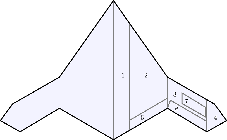
The planform, showing surfaces numbered 1 to 7, is shown in Figure 1 and is based on the X47-B model [9]. Table 2 lists the geometric data for the surfaces. Of some technical significance in this study is the distinct finding of a mathematical relationship between the offset command and the gain of the UCAV x-component guidance controller. The finding marks a pivotal starting point towards advanced formation systems that allow smooth formation changes during flights between manned-unmanned and unmanned-unmanned vehicles. This relationship should be applicable to various UCAVs. Investigating this finding, or similar studies, further can lead to a generalized mathematical relationship that fits various formations and, potentially, different vehicle types.
Table 2. Detailed Geometry Based on Part Layout [9].
Wing Part |
||||
|---|---|---|---|---|
Parameter |
1 |
2 |
3 |
4 |
c, base chord (m) |
11.64 |
9.05 |
2.20 |
2.20 |
ζ, standard mean chord (m) |
10.35 |
5.63 |
2.20 |
1.10 |
b/2, half wingspan (m) |
1.26 |
3.33 |
3.25 |
1.63 |
S, wing gross area (m2) |
26.02 |
37.45 |
14.32 |
3.58 |
$$ {\mathrm{\Lambda }}_{\mathrm{L}\mathrm{E}} $$, leading edge sweep (°) |
56.0 |
56.0 |
30.0 |
56.0 |
$$ {\mathrm{\Lambda }}_{\frac{\mathrm{ϲ}}{4}} $$, quarter chord sweep (°) |
44.1 |
44.1 |
30.0 |
23.6 |
Γ, dihedral (°) |
0 |
0 |
0 |
0 |
λ, taper ratio |
0.78 |
0.24 |
1 |
0 |
Inner twist (°) |
0 |
0 |
0 |
0 |
Outer twist (°) |
0 |
0 |
0 |
0 |
t/c, relative thickness (%) |
16 |
10 |
10 |
10 |
Parameter |
Complete Wing |
|||
b, wingspan (m) |
18.93 |
|||
S, wing gross area (m2) |
81.37 |
|||
AR, aspect ratio |
4.40 |
|||
ζ, standard mean chord (m) |
4.30 |
|||
ζ̅, mean aerodynamic chord (m) |
6.69 |
|||
Control Surfaces |
||||
Parameter |
5 (elevator) |
6 (elevon) |
7 (spoiler) |
|
c, chord (m) |
0.62 |
0.62 |
0.66 |
|
b, wingspan (m) |
3.32 |
3.25 |
2.00 |
|
S, reference area (m2) |
2.05 |
2.00 |
1.32 |
|
The next section gives the control design methodology, including the stability augmentation system, the flight control system, and the guidance system. Section 3 provides a critical assessment of the autopilot, presents the chosen control gains, and shows the simulation test results of the proposed system. In the final section, conclusions are drawn.
2. Methodology
The design is based on models of the flight dynamics of the two aircraft and is subject to the following assumptions:
- -
Flat Earth.
- -
Both aircraft are rigid bodies with six Degrees-Of-Freedom (6DOF).
- -
The UCAV forces and moments act with respect to the Body Axes Centre (BAC).
- -
Both aircraft are initially in formation.
- -
A delay-free communication channel is available, so the UCAV knows the F-16 position.
- -
Both aircraft have constant mass.
The communication channel assumption was made because this paper focuses on investigating the formation guidance system and not to model the complexities of contested communication environments. By abstracting communication to an idealized channel, we can isolate the control-law contributions without conflating them with link-level effects. This modelling choice is common in early-stage guidance research, with robustness to latency and packet loss typically addressed in follow-on studies.
The BAC and any axes notation used in this paper are as they were used in [10]. These are the same notations used by Cook [11].
The F-16 model and flight control system are from [12], and the MATLAB/Simulink models are from [13] and [14]. The UCAV model information is from [15]. The models were analysed and verified, see [9] for details. The F-16 flight control system inputs are the throttle level, elevator deflection, rudder deflection, aileron deflection, and leading-edge flat deflection. The outputs are set to be true airspeed, sideslip angle, angle of attack, quaternions, body angular rates, and earth coordinate positions ($$ {P}_{e} $$), power level, and body accelerations. More details can be found in Appendix D in [10].
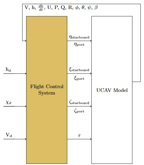
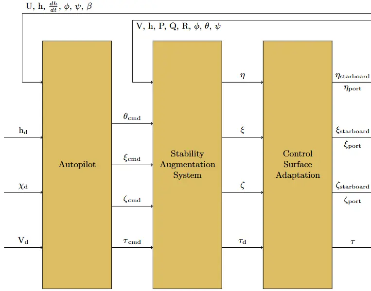
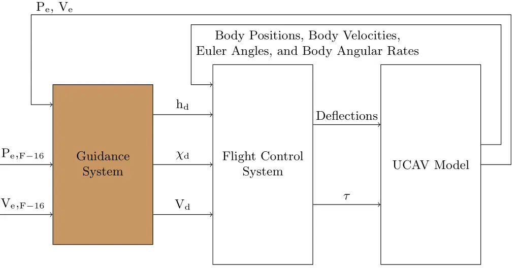
The UCAV flight control system and model architecture is shown in Figure 2 below. The UCAV control system was designed with three main components: Autopilot, Stability Augmentation System, and Control Surface Adaptation. This internal architecture is shown in Figure 3.
The main improvements were made on three out of the five controller loops in the autopilot. These specific three controllers were most improved because they concern the formation guidance system the most. These are the autothrottle, altitude controller, and heading angle controller. The inputted desired commands are the altitude ($$ {h}_{d} $$), heading angle ($$ {\chi }_{d} $$), and true airspeed ($$ {V}_{d} $$) while the outputs are the pitch command ($$ {\theta }_{cmd} $$), roll command ($$ {\varphi }_{cmd} $$), and throttle level command ($$ {\tau }_{cmd} $$), respectively.
The two other controller loops in the autopilot are for the sideslip and roll angles. The input to the sideslip angle, $$ \beta $$, controller is the feedback sideslip angle value from the UCAV model. The sideslip angle command is fixed within the autopilot to zero. The output of this controller is the spoiler deflection command, $$ {\zeta }_{cmd} $$, which is part #7 in Figure 1. The roll angle, $$ \varphi $$, controller input is the roll command outputted from the heading angle controller to account for the lateral/directional coupling effect. The output of this controller is the elevon deflection command, $$ {\xi }_{cmd} $$, which is part #6 in Figure 1. Both controllers follow the PID approach, details are in Section 3.1.
The pitch angle, elevon deflection, spoiler deflection, and throttle level commands are the autopilot outputs inputted into the Stability Augmentation System (SAS) designed by Rodríguez-Miranda as shown in Figure 3 [9,16]. The SAS determines its output based on the inputted commands, feedback variables, gain scheduled lookup tables created by Rodríguez-Miranda, and the desired deflection and throttle level values set within the SAS block. From this, the system outputs the elevator deflection ($$ \eta $$), elevon deflection, spoiler deflection, and throttle level demand ($$ {\tau }_{d} $$) values needed for the control surface adaptation to act. For clarity, the control surface adaptation acts like a simulated actuator [9]. Also, the feedback variables include the true airspeed ($$ V $$), altitude ($$ h $$), vertical speed $$ \left(dh/dt\right) $$, velocity relative to the body x-direction ($$ U $$), and body angular rates ($$ P, Q, R $$).
In addition to Rodríguez-Miranda’s verification of the UCAV model and Duran’s of the UCAV fight control system, another verification was done on both UCAV parts by Alhosani in [10].
A guidance system is designed with along-track, cross-track, and vertical-track PID controllers to minimise the offset errors between the aircraft. Equation (1) shows the general PID control method mathematically.
Determining the control method for the guidance formation system that is both practical and implementable was difficult. Lohani et al. note that PID-based fixed-wing UAV autopilots are easier to implement in practice relative to other control methods [17]. For example, research highlights that the Model Predictive Control (MPC) has larger memory footprint and computational load than PID controllers [18].
More importantly, a PID controller is easier to meet international safety standards and certification requirements. This is especially the case for complex manoeuvres of manned-unmanned formations. This is because the pilot’s safety on the manned aircraft will be considered as the highest priority. Considering the ease of implementation, safety, and certifications, a PID-controlled guidance formation system shows to be the most practical approach for this study.
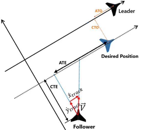
The practicality of such a guidance system is exemplified in Figure 4. To elucidate, the along-track error (ATE) and cross-track error (CTE) are controlled so that the formation guidance system drives the UCAV towards the desired along-track offset (ATO) and cross-track offset (CTO). The time derivatives of ATE and CTE are $$ {\stackrel{˙}{\mathrm{x}}}_{\mathrm{t}\mathrm{r}\mathrm{a}\mathrm{c}\mathrm{k}} $$ and $$ {\stackrel{˙}{\mathrm{y}}}_{\mathrm{t}\mathrm{r}\mathrm{a}\mathrm{c}\mathrm{k}} $$, respectively.
| ```latexK\left(t\right)={k}_{p}e\left(t\right)+{k}_{i}{\int }_{0}^{t}e\left(\tau \right)d\tau +{k}_{d}\frac{de\left(t\right)}{dt}``` | (1) |
The PID gains for each of the tracking controllers (ATE, XTE, VTE) are given in Section 3.2. The gains were hand-tuned for each control loop.
The initial values for the hand-tuning were obtained by solving a sequence of minimization problems for the ATE, XTE, and VTE loops in turn. A measure of the tracking error is defined for a particular manoeuvre as the integral absolute error of the tracking error over the manoeuvre, plus the minimum tracking error, plus the final time tracking error. The chosen manoeuvre was for around 300 m climb and a 500 m turn [10]. This simulation test case was chosen because it is challenging but representative and tests all three tracking loops. The P, I, and D gains are then obtained sequentially by minimizing the tracking error measure using a simple line search for each. The approach is rapid and easy, and gives good initial values for the hand-tuning. More details are in Alhosani [10].
After using the algorithm, the gains are hand-tuned until an acceptable response is reached. This whole process can only work on one controller at a time. An example of this initial design process is shown in Section 3.2 for the along-track controller. The guidance controller inputs and outputs are shown in Table 3.
The inputs ATE, CTE, and VTE are abbreviations to the Along-Track Error, Cross-Track Error, and Vertical-Track Error, respectively. These errors are calculated using Equation (2), Equation (3), Equation (4), Equation (5) and Equation (6) [10]. The variables P, V, and χ in Figure 5 and the equations below refer to position, true airspeed, and heading, respectively. The subscripts “e” denotes an inertial axis system, and the subscript “err” is the error relative to the command. The position error contributes to reducing the formation errors. The velocity error contributes to maintaining the same velocity as the F-16 once it reaches the commanded position offset.
| ```latex{\chi }_{F-16}=\mathrm{atan}\left(\frac{{V}_{north}}{{V}_{east}}\right)``` | (2) |
| ```latex{P}_{err}={P}_{e,UCAV}-{P}_{e,F16}``` | (3) |
| ```latex{V}_{err}={V}_{e,UCAV}-{V}_{e,F16}``` | (4) |
| ```latex\left[\begin{array}{c}ATE\\ CTE\\ VTE\end{array}\right]=\left[\begin{array}{ccc}\mathrm{c}\mathrm{o}\mathrm{s}\left({\chi }_{F16}\right)& -\mathrm{s}\mathrm{i}\mathrm{n}\left({\chi }_{F16}\right)& 0\\ \mathrm{s}\mathrm{i}\mathrm{n}\left({\chi }_{F16}\right)& \mathrm{c}\mathrm{o}\mathrm{s}\left({\chi }_{F16}\right)& 0\\ 0& 0& 1\end{array}\right]{P}_{err}``` | (5) |
| ```latex\left[\begin{array}{c}{\stackrel{˙}{\mathrm{x}}}_{\mathrm{t}\mathrm{r}\mathrm{a}\mathrm{c}\mathrm{k}}\\ {\stackrel{˙}{y}}_{\mathrm{t}\mathrm{r}\mathrm{a}\mathrm{c}\mathrm{k}}\\ {\stackrel{˙}{z}}_{\mathrm{t}\mathrm{r}\mathrm{a}\mathrm{c}\mathrm{k}}\end{array}\right]=\left[\begin{array}{ccc}\mathrm{c}\mathrm{o}\mathrm{s}\left({\chi }_{F16}\right)& -\mathrm{s}\mathrm{i}\mathrm{n}\left({\chi }_{F16}\right)& 0\\ \mathrm{s}\mathrm{i}\mathrm{n}\left({\chi }_{F16}\right)& \mathrm{c}\mathrm{o}\mathrm{s}\left({\chi }_{F16}\right)& 0\\ 0& 0& 1\end{array}\right]{V}_{err}``` | (6) |
The outputs are the guidance demands, which are added to their corresponding autopilot commands so that the autopilot controllers consider the desired formation offset. The demands are represented with a subscript “d”. This means that $$ {V}_{d} $$ is added to the autopilot $$ V $$ command before it enters the autothrottle. Similarly, $$ {\chi }_{d} $$ and $$ {h}_{d} $$ are added to the autopilot heading angle and altitude commands, respectively, before they are inputted into their corresponding controllers. These summations are made in the flight control system block (see Figure 5). The variables fed back into the guidance system are the UCAV positions and velocities. The other two guidance inputs are the F-16 positions and velocities, which are assumed to be from the communication block. The three tracking controllers reside inside the guidance block. A more detailed architecture and explanation of the UCAV system is in [10].
The guidance system was tested through a desktop simulation test under standard manoeuvres with and without wind gusts. Specifically, a joystick was used to control the F-16’s path in a simulation to test how the UCAV maintains its commanded formation using the guidance system. Test results are presented based on the following test cases:
Combining a climb and a turn manoeuvre without a wind gust.
Combining a climb and a turn manoeuvre with a wind gust.
These are shown in [10]. MATLAB/Simulink was the primary tool for these tasks.
3. Results
3.1. Critical Assessment of the UCAV Autopilot
Note that an assessment and corrections were also conducted on the UCAV model. Other adjustments were also made to include wind disturbances in the study. Details are in [10].
To critically assess the UCAV autopilot, commands were used to push the controllers to their limits. The five autopilot PID controllers seemed to work as expected; however, flaws and areas for improvement were found. It is noteworthy to mention that the results began to not work as expected when the commands were pushed to their limits.
Before modifications were made, it was observed that the autothrottle used Mach number ($$ M $$) and speed of sound ($$ a $$) to compute the body x-velocity [16]. Nonetheless, $$ M $$ and $$ a $$ should be used to compute the airspeed as shown in Equation (7) [10]. This was corrected to eliminate systematic errors in the autothrottle.
| (7) |
Furthermore, the heading angle controller used the yaw angle instead of the heading angle pre-modifications [16]. While negligible under coordinated flight ($$ \beta \approx 0 $$), this design could lead to confusion or inaccuracies in future scenarios where sideslip is nonzero. The controller was updated to use heading angle directly, ensuring a more robust and interpretable design [10].
Additionally, there was an inconsistency between how $$ V $$ was computed in the autopilot versus the plant ISA model, due to differing atmospheric models [16]. This discrepancy, although small (<0.01%), was resolved by harmonizing both with the same set of standard atmospheric equations [10]. These are Equation (8), Equation (9) and Equation (10) [19]. The other minor adjustments made to the autopilot are mentioned in [10]. After fixing several autopilot parts, the main response improvements were via controller-tuning. Table 4 shows the resulting gains and units.
| (8) | |
| (9) | |
| ```latex T=\begin{cases}288.15-0.0065h\,\,\forall\,\,(0\leq h<11)\\\,\,\,\,\,\,\,\,\,\,\,\,216.25\,\,\forall\,\,(11\leq h<25)\\196.65+0.0010h\,\,\forall\,\,(25\leq h<32)\\\,\,\,\,\,\,\,\,\,\,139.05-0.0028h\,\,\forall\,\, h\geq32&\end{cases}``` | (10) |
The equations above denote temperature, specific heat ratio, and universal gas constant as $$ T $$, $$ \gamma $$, and $$ R $$ and with units of K, [-], and J/kg/K, respectively. The specific heat ratio is 1.4, and the universal gas constant is 287 J/kg/K. The altitude in the atmospheric equations is km.
Moreover, the anti-windup gain in the autothrottle was modified from 1000 m/s to 699.3 m/s. As for the altitude controller, a low-pass filter was added. This lead-lag filter had a cutoff frequency of 0.005 rad/s; thus, a small range of frequencies were allowed to pass while high frequencies were attenuated. This smoothened out the controller response by eliminating noisy signals.
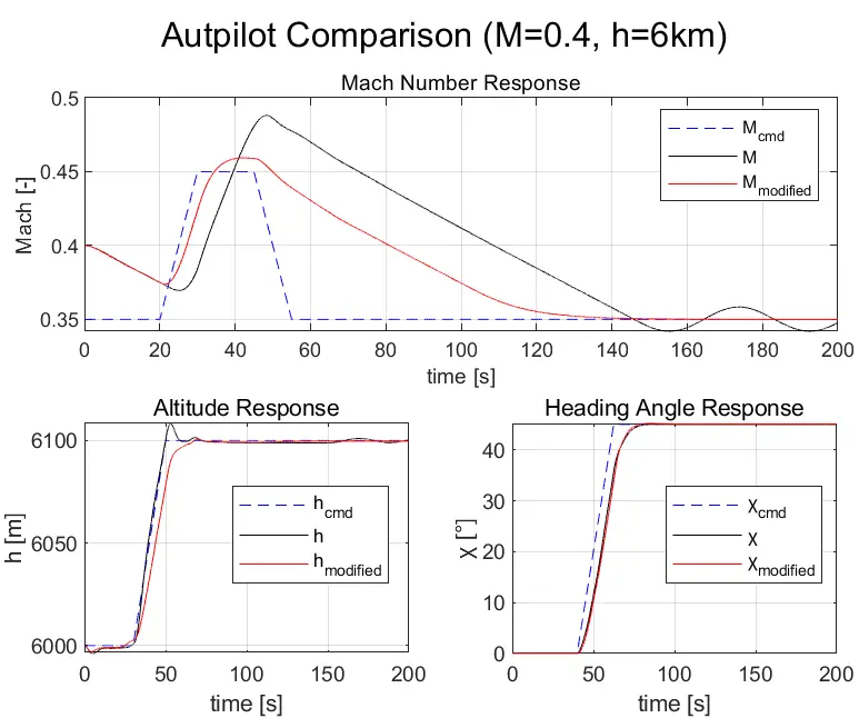
These modifications showed enhanced responses. For instance, the altitude controller is now able to handle a ramp command with a slope of 20 m/s instead of the original altitude controller’s maximum ramp command slope of 5 m/s.
Figure 6 compares both autopilots under varying commands from 19 s until 56 s. Between 30 s and 55 s, the varying commands are all simultaneously changing. These responses portray the modified autopilot enhancements [10]. The modified autopilot has less overshoot, less oscillations, and a more accurate response relative to the unmodified autopilot.
3.2. Formation Guidance System
The improved autopilot is used in the guidance system. Keep in mind that the formation offset position of the UCAV relative to the F-16 is [−20, 10, 0] m and will be considered throughout the paper.
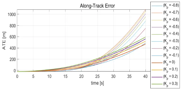
It was difficult to determine the initial gain values to start hand-tuning from. Due to this challenge, an algorithm was built to provide an approximated initial gain value. The guidance system was initially designed using the algorithm, which was briefly explained in Section 2. The design analysis algorithm was done on each of the controllers. The algorithm’s first-step result for the along-track controller is shown in Figure 7.
The algorithm was also used to determine the I and D gains as described in Section 2. The along-track controller algorithm results are shown in Table 5. This algorithm was developed due to the ambiguity of the starting point gain values for the hand-tuning approach.
A comprehensive illustration and discussion of the design results are in Section 4.2.1 and appendix E of [10].
Typically, a vertical-track controller is unnecessary if there is an altitude autopilot. Nonetheless, it was added for a better vertical performance as shown in Figure 8 [10]. Furthermore, the final gains reached through hand-tuning are shown in Table 6.
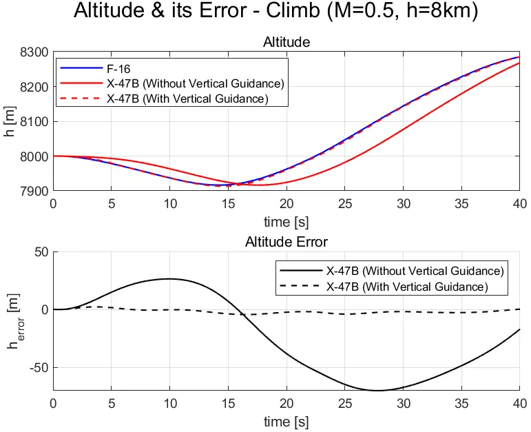
The addition of a vertical guidance controller almost eliminated the error that existed when only using the altitude autopilot. It is observed that without the vertical tracker, the maximum error reached is more than 50 m. On the other hand, the inclusion of a vertical tracker reduced the maximum error to less than 5 m. The vertical-track controller adjusts the altitude command to ensure lower vertical errors. The figure above illustrates these altitude errors, using the same climb and turn manoeuvre test case without wind. This led to a more robust vertical system.
After finalizing the guidance system, the joint stick desktop simulation testing was conducted. This was done for a Mach = 0.5 and h = 8000 m during a climb with a turn. The cases with and without gust were tested.
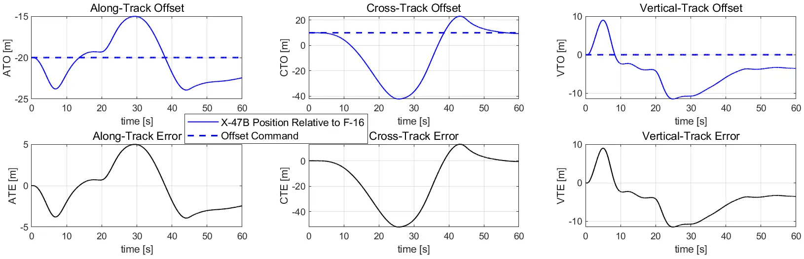
Figure 9 shows the case without a wind gust. The along-track controller response portrays stability by maintaining a relatively low ATE. The stability is also shown at the end of the response, where the along-track offset gradually returns to the command line.
As for the cross-track controller response, it illustrates the difficulty of handling the east turn done by the F-16. This is shown by the UCAV going 40 m to the west to prepare doing the same east turn. This is more of a robustness problem than a stability one because the response demonstrates to eventually come back close to the command line.
The vertical-track controller response shows a relatively small maximum error of around 11 m. It portrays a struggle in sticking with the command line. However, the small VTE maintained throughout the simulated test illustrates stability.
The ATE initially has a relatively small error until the gust is introduced at 15 s. Thus, the ATE magnitude increases with time, meaning the UCAV moves away from the F-16 along their relative x-direction. Following the ATO command until the gust is present indicates that the guidance system is stable when there is no disturbance and becomes more unstable when injected. This is a robustness problem that can be resolved with more sophisticated methods.
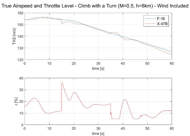
It was thought that a potential reason for the continuous along-track deviation after a wind gust is the UCAV thrust limitation relative to the F-16 thrust. Although this could have played a role since the maximum F-16 thrust is higher than that of the UCAV, another reason comes up when looking at the true airspeed.
Figure 10 shows that the thrust did not reach its upper limit while the UCAV true airspeed was almost always close to the F-16 true airspeed [10]. This indicates that the autothrottle has a higher control authority than that of the along-track controller. This can be resolved by optimizing the trade-off between the control authority of the autothrottle and the along-tracker.
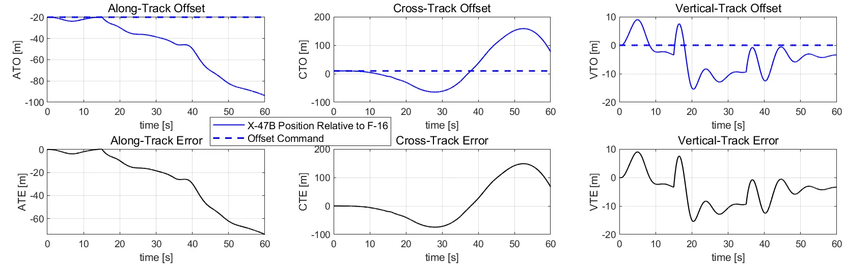
Figure 11 shows the test results with wind disturbance. It will demonstrate how the response in the vertical axis is the most robust compared to the response in the other axes. Specifically, the gust vectors, [$$ \begin{array}{ccc}-3& 5& -15\end{array} $$] m⋅s−1 and [$$ \begin{array}{ccc}2& -4& -10\end{array} $$] m⋅s−1, were applied at times 15 s and 35 s, respectively. The wind disturbances were purposely chosen at these magnitudes and timings to push the guidance system to its boundaries. This allowed the observance of the system under a challenging condition.
As for the CTE, the UCAV had to make a turn with the F-16 at around 10 s, but the F-16 turn was too sharp for the UCAV to handle. This made the UCAV turn to the opposite direction first so that it can pull higher g’s as it switched directions to follow the F-16 turn. As it tried to pull g’s for the turn, the gust disturbance hit it and caused it to deviate further away from the leading aircraft. Corresponding to the UCAV behaviour when there was no gust, as portrayed in Figure 9, the UCAV shows a similar behaviour of gradually converging to a steady state after it was hit by the wind. This shows that although the cross-track controller is stable, the controller is not robust enough to handle such a turn. Similarly to the ATE situation, this is a robustness problem.
Moreover, the VTE showed stronger stability since it did not deviate much from the vertical-track offset (VTO). It also gradually shows a quick return to the steady state. This demonstrates that the vertical-track controller robustness is higher than the along-track and cross-track controllers.
3.3. Distinct Result
Although the along-track controller could be improved, the study provided the following unique finding. It is an empirical mathematical relationship that connects the along-track controller offset command with its gain. The relationship is shown as Equation (11) [10].
| ```latex{K}_{new}=\frac{K}{\left|AT{O}_{cmd}\right|}``` | (11) |
The new set of PID gains is denoted as $$ {K}_{new} $$. The set of PID gains designed for a formation offset of [−20, 10, 0] m is denoted as K. Table 7 shows how this relationship was used in the controller.
Table 7. Gain-Command Relationship [10].
Guidance Controllers |
Adjustable Gains for Varying ATO Commands (10−3) |
||
|---|---|---|---|
```latex{\bm{k}}_{\bm{p}}``` |
```latex{\bm{k}}_{\bm{i}}``` |
```latex{\bm{k}}_{\bm{d}}``` |
|
Along-Track |
$$ \frac{-13.85}{\left|\mathrm{A}\mathrm{T}{\mathrm{O}}_{\mathrm{c}\mathrm{m}\mathrm{d}}\right|} $$ s−1 |
$$ \frac{-0.42}{\left|\mathrm{A}\mathrm{T}{\mathrm{O}}_{\mathrm{c}\mathrm{m}\mathrm{d}}\right|} $$ s−2 |
$$ \frac{0}{\left|\mathrm{A}\mathrm{T}{\mathrm{O}}_{\mathrm{c}\mathrm{m}\mathrm{d}}\right|} $$ |
This relationship can also be used to find the ATO command from the UCAV gain as well. As the ATO command magnitude increases, the along-track gains are decreased by a factor equal to the increased ATO command magnitude. This is a firm relationship that also works for large distances (see Figure 12).
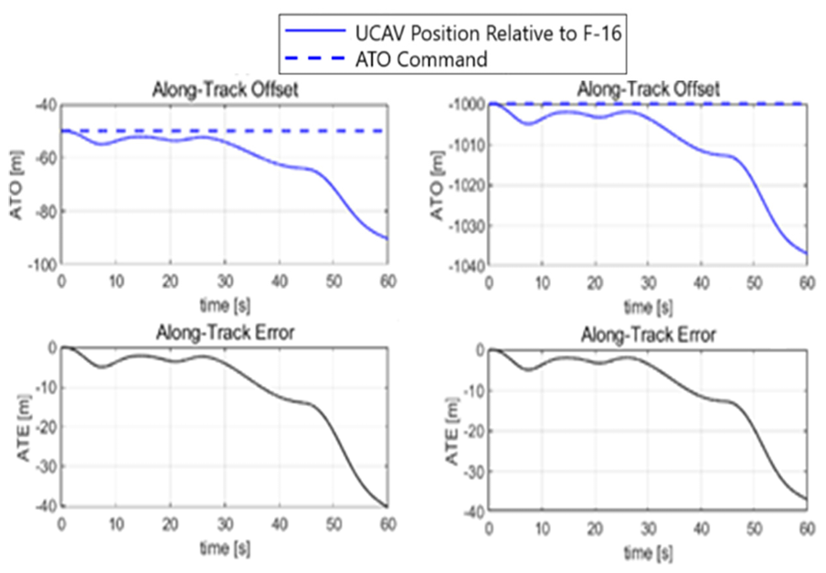
The ATE of the 50 m and the 1000 m ATO commands is almost the same within 60 s. Due to the relationship, the error was maintained even for large offset commands.
Using this distinct finding will not result in a huge difference relative to the gain scheduling method for example. Nevertheless, the advantage of this distinct finding is that it is easily implementable compared to other gain determining methods in formation systems.
4. Conclusions and Further Work
This study presented the design and testing of a formation guidance system for a UCAV acting as a wingman to a manned F-16 fighter jet. It began with improving the provided autopilot so that the guidance system can be more accurate with it.
The gains of the guidance controllers were initially calculated using an optimization algorithm. Afterwards, the PID-based formation guidance system was hand-tuned and demonstrated stability during desktop simulations, particularly in the vertical (z) direction, where it exceeded expectations. However, robustness drawbacks in the along-track (x) and cross-track (y) directions were observed. The PID method was selected for its ease of implementation and ease of compliance with safety standards and certifications for when there are manned aircraft working with unmanned aircraft. A key finding was the novel mathematical relationship between the along-track offset command and its gains, providing a basis for advanced formation systems.
The controller robustness could be improved by means of adaptive control or model-based techniques. For example, [20] proposes techniques for robust flight control using sliding mode control; such methods can be used for this problem. Another approach for improving the robustness is to adopt the Fractional Order PID (FOPID) method [21]. A comparative study comparing the methods proposed in [22], where the design and analysis of a tracking guidance system for the purpose of air-to-air refuelling were presented, should be performed.
A formal stability and comprehensive robustness analyses also need to be done. This could include the mass variation during flight. This may require additional gain-scheduling. Note that the gain-offset relationship found in this paper is focused on the along direction for the specified UCAV model. Research in this matter can be further investigated to discover a gain-offset relationship in the cross and vertical directions of similar UCAV models. Concentrating on finding a generalized gain-offset relationship in this part of the formation guidance and control field is the way to move forward and adapt to emerging technologies. Empowering and advancing this focused part of the field can enable various UAVs with mathematical relationships that can replace gain scheduling.
The paper considered only the problem of a single wingman. The approach can be extended to multiple wingmen. This introduces the problem of dynamic role-switching and formation changes. For example, Wang et al. investigated consensus tracking over asynchronous cooperation–competition networks, where agents can switch between cooperative and competitive interactions while still achieving stable group behavior [6]. Although the problem of autonomous vehicle swarms has been extensively investigated, the problem when there are also manned aircraft in the formation is fairly open.
The proposed design makes several assumptions; an important one is delay-free communication. Communication delays can reduce stability margins, and this should be analysed. For example, the impact of the full communication model on the formation guidance system is demonstrated in [23]. Hence for further work, the guidance system should be validated under bounded delays and packet-loss communication models.
Acknowledgment
Thanks is extended to the company, Halcon, for their funding assistance.
Author Contributions
Conceptualization, F.A.A. and J.F.W.; Methodology, F.A.A.; Software, F.A.A.; Validation, F.A.A.; Formal Analysis, F.A.A.; Investigation, F.A.A.; Resources, J.F.W.; Data Curation, J.F.W.; Writing—Original Draft Preparation, F.A.A. and J.F.W.; Writing—Review & Editing, F.A.A. and J.F.W.; Visualization, F.A.A. and J.F.W.; Supervision, J.F.W.
Ethics Statement
Not applicable.
Informed Consent Statement
Not applicable.
Data Availability Statement
The software and data used for this paper are available from the second author, J.F.W, on request.
Funding
This research received no direct external funding.
Declaration of Competing Interest
The authors declare that they have no known competing financial interests or personal relationships that could have appeared to influence the work reported in this paper.
References
-
Nowacki G, Bolz K. Challenges and Threats of Unmanned Aerial Vehicles for Aviation Transport Safety. J. Civ. Eng. Transp. 2022, 4, 9–21. [Google Scholar]
-
Jordan J. The Future of Unmanned Combat Aerial Vehicles: An Analysis Using the Three Horizons Framework. Futures 2021, 134, 102848. [Google Scholar]
-
Li Y, Qiu X, Liu X, Xia Q. Deep Reinforcement Learning and Its Application in Autonomous Fitting Optimization for Attack Areas of UCAVs. J. Syst. Eng. Electron. 2020, 31, 734–742. [Google Scholar]
-
Waydo S, Hauser J, Bailey R, Klavins E, Murray RM. UAV as a Reliable Wingman: A Flight Demonstration. IEEE Trans. Control. Syst. Technol. 2007, 15, 680–688. [Google Scholar]
-
Zhang J, Wang D, Yang Q, Shi Z, Ji L, Shi G, et al. Loyal Wingman Task Execution for Future Aerial Combat: A Hierarchical Prior-Based Reinforcement Learning Approach. Chin. J. Aeronaut. 2024, 37, 462–481. [Google Scholar]
-
Li W, Yan S, Shi L, Yue J, Shi M, Lin B, et al. Multiagent Consensus Tracking Control Over Asynchronous Cooperation–Competition Networks. IEEE Trans. Cybern. 2025, 55, 4347–4360. [Google Scholar]
-
Alhosani FA, Whidborne JF. Formation Guidance System for an Unmanned Combat Aerial Vehicle as a Wingman to an F-16. In Proceedings of the 1st International Conference on Drones and Unmanned Systems (DAUS’ 2025), Granada, Spain, 19–21 February 2025; pp. 260–265. [Google Scholar]
-
X-47B UCAS. Available online: https://www.northropgrumman.com (accessed on 1 June 2023). [Google Scholar]
-
Rodríguez-Miranda I. Modelling and Simulation of a Flying Wing. Master’s Thesis, Cranfield University, Cranfield, UK, 2011. [Google Scholar]
-
Alhosani FA. Designing and Testing a Formation Guidance System for an X-47B as a Wingman to an F-16. Master’s Thesis, Cranfield University, Cranfield, UK, 2023. [Google Scholar]
-
Cook MV. Flight Dynamic Principles; Butterworth-Heinemann: Oxford, UK, 1997. [Google Scholar]
-
Nguyen LT, Ogburn ME, Gilbert WP, Kibler KS, Brown PW, Deal PL. Simulator Study of Stall/Post-Stall Characteristics of a Fighter Airplane with Relaxed Longitudinal Static Stability; NASA Langley Research Center: Hampton, VA, USA, 1979. [Google Scholar]
-
Sonneveldt L. Nonlinear F-16 Model Description, Control & Simulation Division; Delft University of Technology: Delft, The Netherlands, 2010. [Google Scholar]
-
Sonneveldt L, Van Oort ER, Chu QP, Mulder JA. Nonlinear Adaptive Trajectory Control Applied to an F-16 Model. AIAA J. Guid. Control. Dyn. 2009, 32, 25–39. [Google Scholar]
-
X-47B UCAS. Datasheet; Northrop Grumman: Falls Church, VA, USA, 2015. [Google Scholar]
-
Duran CM. Design of a Cruise Flight Control System for a Tailless Flying Wing. Master’s Thesis, Cranfield University, Cranfield, UK, 2017. [Google Scholar]
-
Lohani TA, Dixit A, Agrawal P. Adaptive PID Control for Autopilot Design of Small Fixed Wing UAVs (Aerosonde UAV). In Proceedings of the MATEC Web of Conferences—2nd International Conference on Sustainable Technologies and Advances in Automation, Aerospace and Robotics, Sehore, India, 15–16 December 2023; Volume 393, Paper no. 03005. [Google Scholar]
-
Di Cairano S, Kolmanovsky IV. Real-Time Optimization and MPC in Aerospace; MERL Tech. Report TR2018-086; Cambridge, MA, USA, 2018. [Google Scholar]
-
Glenn Research Center. NASA. Available online: https://www.grc.nasa.gov/www/k-12/airplane/atmosmet.html (accessed on 2023). [Google Scholar]
-
Alwi H, Edwards C. Fault Tolerant Control Using Sliding Modes with On-Line Control Allocation. Automatica 2008, 44, 1859–1866. [Google Scholar]
-
Abdulridha NM, Mary AH, Jasim HH. Optimized PID, FOPID and PIDD2 for Controlling UAV Based on SSA. Am. Sci. Res. J. Eng. Technol. Sci. 2023, 92, 77–90. [Google Scholar]
-
Qureshi S. The Design of a Trajectory Following Controller for Unmanned Aerial Vehicles. Master’s Thesis, Cranfield University, Cranfield, UK, 2008. [Google Scholar]
-
Shi J, Yan S, Li W. Consensus and Products of Substochastic Matrices: Convergence Rate with Communication Delays. IEEE Trans. Syst. Man Cybern. Syst. 2025, 55, 4752–4761. [Google Scholar]