Detection and Classification of Faults in a
Photovoltaic System—A New Hybrid Algorithm

Abdullah, Muhammad; Shah, Muhammad Qasim; Habib, Kashif; Kabeer, Fajar; Shakir, Muhammad Basit; Zainab, Rida; Sekh, Abdul Kader

doi:10.70322/ces.2025.10014

lssue 4, Volume 3

Part of Special Issue: Modeling, Control, Optimization, and Diagnostics of Photovoltaic Systems

Article Open Access

Detection and Classification of Faults in a Photovoltaic System—A New Hybrid Algorithm

Muhammad Abdullah ^1,* Muhammad Qasim Shah ^2,* Kashif Habib ¹ Fajar Kabeer ³ Muhammad Basit Shakir ⁴ Rida Zainab ¹ Abdul Kader Sekh ⁴

Author Information

Other Information

Institute of Electrical, Electronics and Computer Engineering, University of the Punjab, Lahore 54590, Pakistan

Faculty of Science and Technology, Bournemouth University, Poole BH12 5BB, UK

Department of Physics, Government College University, Lahore 54000, Pakistan

⁴

School of Mathematics and Physics, University of Science and Technology, Beijing 100083, China

Authors to whom correspondence should be addressed.

Received: 07 July 2025 Accepted: 12 September 2025 Published: 25 September 2025

Views:693

Downloads:113

Clean Energy Sustain. 2025, 3(4), 10014; DOI: 10.70322/ces.2025.10014

ABSTRACT: Four main types of faults can occur at the DC side of any Photovoltaic System (PVS). These faults are quite dangerous and can cause permanent damage to the photovoltaic modules if not addressed promptly. The faults include open circuit, short circuit, degradation, and partial shading. Short circuit faults are classified into line-to-line (L-L) and line-to-ground (L-G). Detecting these faults requires specialized algorithms. This paper tackles this complex issue through (1) fault-finding equations and the placement of current sensors, and (2) a new hybrid algorithm based on data from the fault-finding equations and current sensors. Numerous simulations using PSIM 2021 were conducted to verify this proposed solution. The hybrid algorithm presented here is original compared to previous studies. It is easy to understand, responds quickly, and can be implemented in systems with photovoltaic arrays of any size.

Keywords: Photovoltaic system faults; PV system fault detection; Open circuit faults; Fault detection and classification

1. Introduction

With the constant increase in green house gas, GHG and CO₂ emissions and the electricity demand, many have shifted their generation from conventional systems to Photovoltaic systems (PVS). As the integration of (PVS) grows, so does the need for fault detection and classification to ensure smooth operation of the (PVS) [1,2,3]. The entire PVS is divided into two parts: one is the DC side and the other is the AC side. On the DC side, the PV array is present along with blocking and bypass diodes. On the AC side, converters and inverters are present [4]. On the DC side, four major types of faults can appear: Degradation, Partial shading, Open circuit, and Short circuit fault. These faults are quite difficult to ignore as they can cause irreversible power loss of the PVS. These faults can also decrease the efficiency of the energy conversion. Many fault detection techniques have been developed to detect the faults so that the PVS can work with maximum possible efficiency. Detection of these faults, particularly on the Photovoltaic (PV) array side, is quite significant. This will improve the efficiency of energy conversion and reduce the cost of maintenance [5,6]. For the protection of the PVS, many have used conventional protection devices like Overcurrent protection (OCPD) and Ground fault protection (GCPD) but as the current-voltage (IV) characteristics of PV modules are nonlinear in nature and due to the presence of blocking diodes in the strings makes it is hard to detect the actual faults successfully [1,7,8]. Many techniques have been published in the past regarding PVS fault detection. Still, the majority used a concept in which the comparison is done among the real-time data with the desired data of the Photovoltaic array. This paper will revolve around the detection and classification of open circuit faults, degradation, partial shading, short circuit faults, and further classification of short circuit faults, whether there is an L-L or L-G fault. In the past, many researchers have proposed different techniques to detect and classify the faults, but the majority of the work addressed related to the detection of PVS faults requires complex algorithms and costly materials. The used methods were statistical, signal-based, artificial intelligence-based, virtual imaging IV curve, sensors, etc. All of the previous fault detection techniques can be divided into six major categories.

1.: Probabilistic/Statistical approach: The basic working principle of these techniques depends upon the comparison between actual or real-time data with the estimated data of the PV array. The setting of thresholds is quite significant for detecting the fault. The fault detection technique [4] employed a statistical test known as the t-test, while the technique [7,8] utilized a simple scientific approach with the aid of formulas to detect faults in a PVS. The major problem with these two techniques is that the number of sensors required is higher, and the equipment and materials used are quite expensive, such as an irradiance sensor. The technique [9] successfully identified the open-circuit fault in the PVS; however, the problem was that it required a spare reference cell to complete the fault detection.
2.: Signal Analysis: Numerous techniques are present for the signal analysis of any given fault condition. These fault-finding techniques are classified as the wavelet packet transform [10,11], autoregressive-based time correlation [6], outlier rules of detection [12,13], Decomposition of multi-resolution signals [14], and a spectrum time domain reflectometry [15].
All these fault detection techniques can successfully detect the fault, but are unable to classify the nature of the fault that occurred in the PVS, except for the technique [16]. Another problem with these approaches is that they require an extra piece of hardware to assist in extracting and computing the PVS features. All of the above techniques will only work in any PV array without the presence of the blocking diodes.
3.: Artificial intelligence: In recent years, artificial intelligence (AI) based fault finding techniques are quite popular. To detect PVS faults several researchers of this domain present many AI techniques. Neural network-based techniques , Another technique that is being used heavily is the K-nearest neighbor (KNN) presented in [17]. Some researchers used Support vector machine (SVM) mentioned in These AI techniques require extensive time to train the systems, and then they can detect the fault that occurred in a PVS. The major drawback is the cost; all of the above techniques can only work with a PV array without blocking diodes.
4.: Virtual imaging-based techniques: These techniques have been presented by many researchers over the years. The techniques [18,19,20] use infrared cameras and thermal imaging to detect the faults in the PVS. The drawbacks of these techniques are that they require continuous monitoring, and the equipment used is quite expensive, so these techniques are not economical.
5.: Sensorless techniques: Some of these techniques use a perturb and observe (P&O) maximum power point tracking MPPT algorithm for extracting the data from the system. A (P&O) technique is presented in [21], and dynamic I-V techniques [22] are also proposed for sensorless fault detection in PVS. The major drawback of these techniques is that they require thresholds, and the system requires setting thresholds manually.
6.: Sensor-based techniques: A sensor-based technique in [23]. This technique is simple and uses two current sensors per string to detect and classify the L-L and L-G faults. The drawback of this is that it is only limited to some specific types of faults which are L-L and L-G. Another sensor-based technique was proposed by [24]. This voltage-based technique can detect and classify the L-L, L-G, and open faults of PVS. But in technique [24], the major drawback comes with controllers interfacing; this only works on a system without blocking diodes.

In this paper, a simple and fast technique is proposed. Fault characteristic ratios will be compared with the thresholds, and two current sensors are employed, one on the top of the first string and the second at the bottom of the last string. This proposed technique is scalable to any array size. This technique not only detects the faults but also classifies them. The faults classified are open fault, shading, degradation, and short fault (L-G, L-L).

2. Materials and Methods

2.1. Fault Analysis The behavior of the PVS is evaluated in this part of the paper. The key elements for the fault analysis are Current and voltage indicators: The ratios of real-time current and voltage values with the given open circuit voltage (Voc) and short circuit current (Isc) ratings of the PV module are denoted by ($$R_{I}$$), ($$ R_{V}$$). Fault characteristic equations: The equations through which we will be able to create the respective fault thresholds. Faults thresholds: The thresholds $$T_{I O} , T_{V S} , T_{I P }$$ which will be compared to the current and voltage indicators ($$R_{I}$$), ($$ R_{V}$$). Data from the two current sensors: Values of current sensors one placed at the top of the first string (Is_up S1) and the second at the bottom of the second string (Is_low S2) in both fault-free and fault conditions. 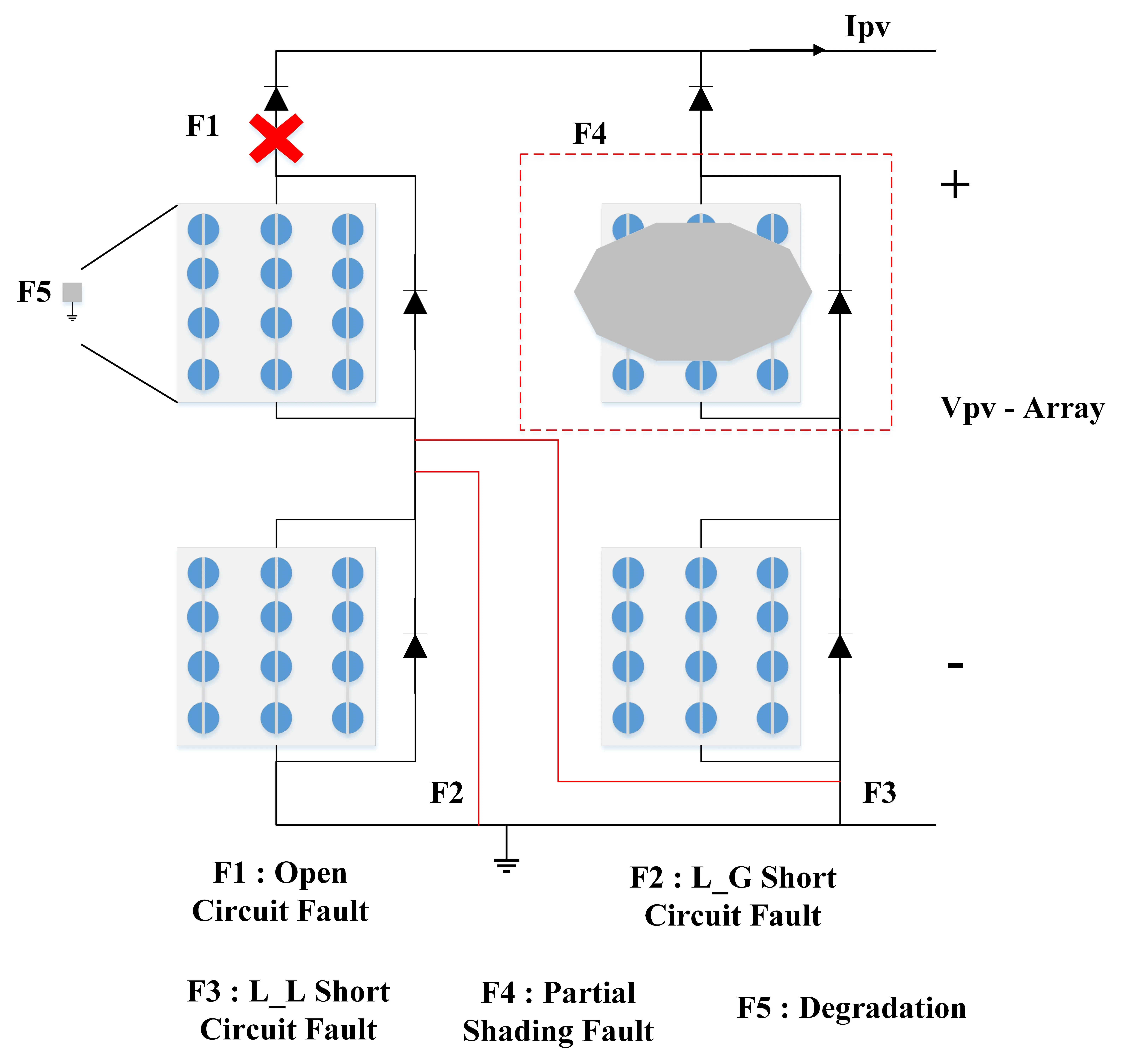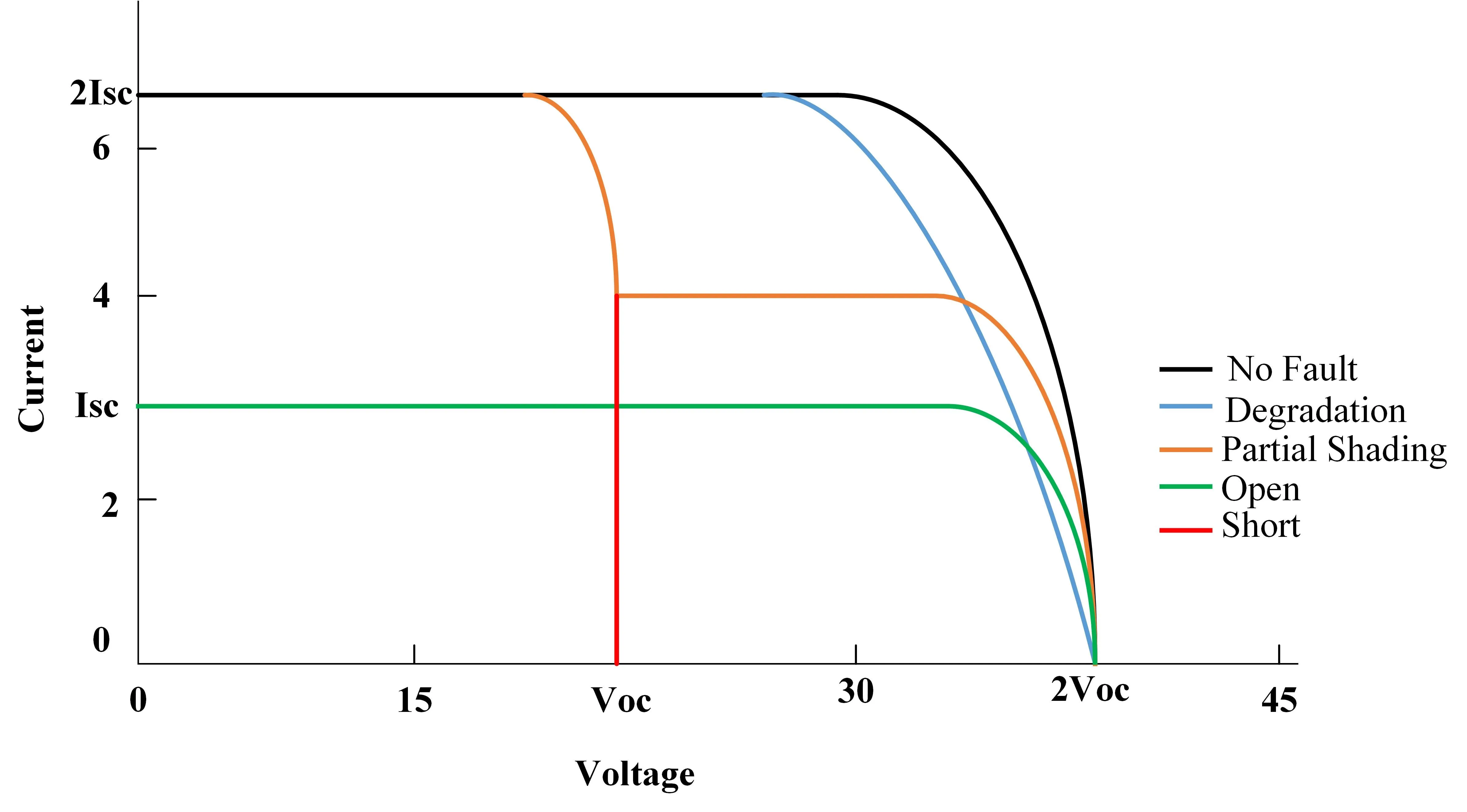Based on these key elements, a new hybrid fault detection and classification algorithm (HFDCA) is proposed, which will increase the number of faults detected and classified as compared to the previous work. This analysis of faults will be divided into 6 parts: degradation, open, shading, short, L-G, and L-L faults in a PVS. The faults discussed are elaborated in Figure 1, and their I-V curves are presented in Figure 2.

Figure 1. The proposed system configuration with faults.

Figure 2. I-V curves for each fault.

A.: Current and Voltage Indicators

To calculate these indicators, a system will be required to give real-time voltage and current values. These can be calculated as [25].

```latexR_{I} = \frac{I}{I s c}```

(1)

```latexR_{V} = \frac{V}{V o c}```

(2)

Here $$ R_{I}$$, $$R_{V}$$ are the indicators used as the current and voltage indicators. $$I$$ is the real-time output current after the operation of Maximum Power Point Tracking (MPPT), $$V$$ is the real-time output voltage. $$I s c$$ is the rated short circuit current and $$V o c$$ is the rated open circuit voltage of the PVS. Both $$I s c$$ and $$V o c$$ can separately be calculated by the following equations.

```latexI s c = N p \left(\frac{I_{s c m \_S T C}}{1000} G + K_{I} \left(T - T_{S T C}\right)\right)```

(3)

```latexV o c = N s \left(V_{o c m \_ S T C} + K_{V} \left(T - T_{S T C}\right) + V_{t} l n \left(\frac{I s c / N p}{I_{s c m \_ S T C}}\right)\right)```

(4)

Here in Equations (3), and (4), $$T_{S T C} $$ is the standard testing temperature which is 25 degrees Celsius and T is the real-time temperature of the PV module. $$K_{I}$$ and $$K_{V}$$ are the temperature coefficients of the current and voltage, respectively. $$I_{s c m \_ S T C}$$ is the rated short circuit, and G is value of irradiation under standard testing conditions. Current at the standard conditions. $$G$$ is the normal irradiance that is 1000 W/m². $$N p$$ is the number of parallel connected PV modules, while $$N s$$ is the number of series connected PV modules, and $$V_{t}$$ is the thermal voltage. By evaluating the above Equation (1) and Equation (2), the current and voltage indicators for the fault scenario are given as

```latexR_{V M} = \frac{V_{M}}{V o c}```

(5)

```latexR_{I M} = \frac{I_{M}}{I s c}```

(6)

Here $$V_{M}$$, $$I_{M}$$ are the output values of the current and the voltage at the maximum power point (MPP) can also be calculated separately as,

```latexI m = N p \left(\frac{I_{m m \_ S T C}}{1000} G + K_{I} \left(T - T_{S T C}\right)\right)```

(7)

Here $$I_{m m \_ S T C}$$ is the current at (MPP) of the PV module at the standard conditions.

```latexV m = N s \left(V_{t} l n \left(1 + \frac{I s c - I m}{I s c} \left(e^{\frac{V o c}{N s V t}}\right)\right) - \frac{I m}{N p} R s\right)```

(8)

Here $$R s$$ is the value of the series resistance.

(A): Fault characteristic equations and fault thresholds.

These equations are significant for the classification of faults in a PVS. Every equation is unique and different for every type of fault.

(1): Open Circuit Fault

Whenever an open circuit fault (OCF) occurs, the current of the PV array drops drastically, and the fault characteristics equation can be formulated as.

```latexR_{I O} = \frac{\left(N p - 1\right)}{N p} \frac{I m}{I s c} = \alpha R_{I M}```

(9)

Here the $$R_{I O}$$ is the current indicator and $$R_{I M}$$ is the indicator for current in a fault-free condition and,

```latex\alpha = 1 - \frac{1}{N p}```

(10)

```latexT_{I O} = \epsilon \alpha R_{I M}```

(11)

Here $$T_{I O }$$ is the open circuit fault threshold value, and $$\epsilon$$ is the allowed offset value used which is 9% in the open circuit fault case. Sensing Signal: In the system, whenever the value of the current indicator $$R_{I}$$ < $$T_{I O}$$ It will indicate that the system has encountered an open circuit fault.

(2): Short Circuit fault

Whenever a Short circuit fault (SCF) occurs, the voltage of the PV array drops drastically, and the fault characteristics equation can be formulated as,

```latexR_{V S} = \frac{\left(N s - 1\right)}{N s} \frac{V m}{V o c} = \beta R_{V M}```

(12)

Here the $$R_{V S}$$ is the voltage indicator and $$R_{V M}$$ is the indicator for voltage in fault-free conditions and,

```latex\beta = 1 - \frac{1}{N s}```

(13)

```latexT_{V S} = \epsilon \beta R_{V M}```

(14)

Here $$T_{V S }$$ is the short circuit fault threshold value. $$\epsilon$$ is the allowed offset value used, which is 8% in short circuit fault case. Sensing signal: In the system, whenever the value of the current indicator $$R_{V}$$ < $$T_{V S}$$ it will indicate that the system has encountered a short circuit fault.

(3): Partial Shading

For partial shading conditions, the fault characteristic equations are given in the form of current and voltage indicators under partial shading conditions.

```latexR_{I P} = \frac{I_{m p}}{I s c}```

(15)

Here $$I_{m p}$$ is the maximum value of current under shading conditions.

```latexR_{m p} = \frac{V_{m p}}{V o c}```

(16)

Here $$V_{m p}$$ is the maximum value of voltage under shading conditions.

```latexT_{I P } = \epsilon R_{I P}```

(17)

Here $$T_{I P }$$ is the shading fault threshold value. Sensing signal: In the system, whenever the value of the current indicator $$R_{I}$$ < $$T_{I P}$$ it will indicate that the system has encountered a shading fault. In Equation (11), Equation (14) and Equation (17) the $$\epsilon$$ represents the allowed offset to the threshold values. In the case of open fault $$\epsilon$$ is 9% while in every other fault condition, it is taken as 8%.

(4): Degradation

Many classifications of degradation faults have been presented before. One of them is an increment in the series resistance of the PV module. Sensing signal: In the system, whenever the value of the current indicator $$R_{I}$$ < $$T_{I O}$$ and $$R_{V}$$ < $$T_{V S}$$ will indicate that the system has encountered a degradation fault.

(B): Data from the two current sensors (Is_up S1), (Is_low S2).

These current sensors will come in handy for further classifying the short circuit fault, whether the fault is L-G or L-L. Whenever the system encounters our algorithm will quickly compare the sensor connected at the top of the first string (Is_up S1) and the sensor connected at the bottom of string 2 (Is_low S2).

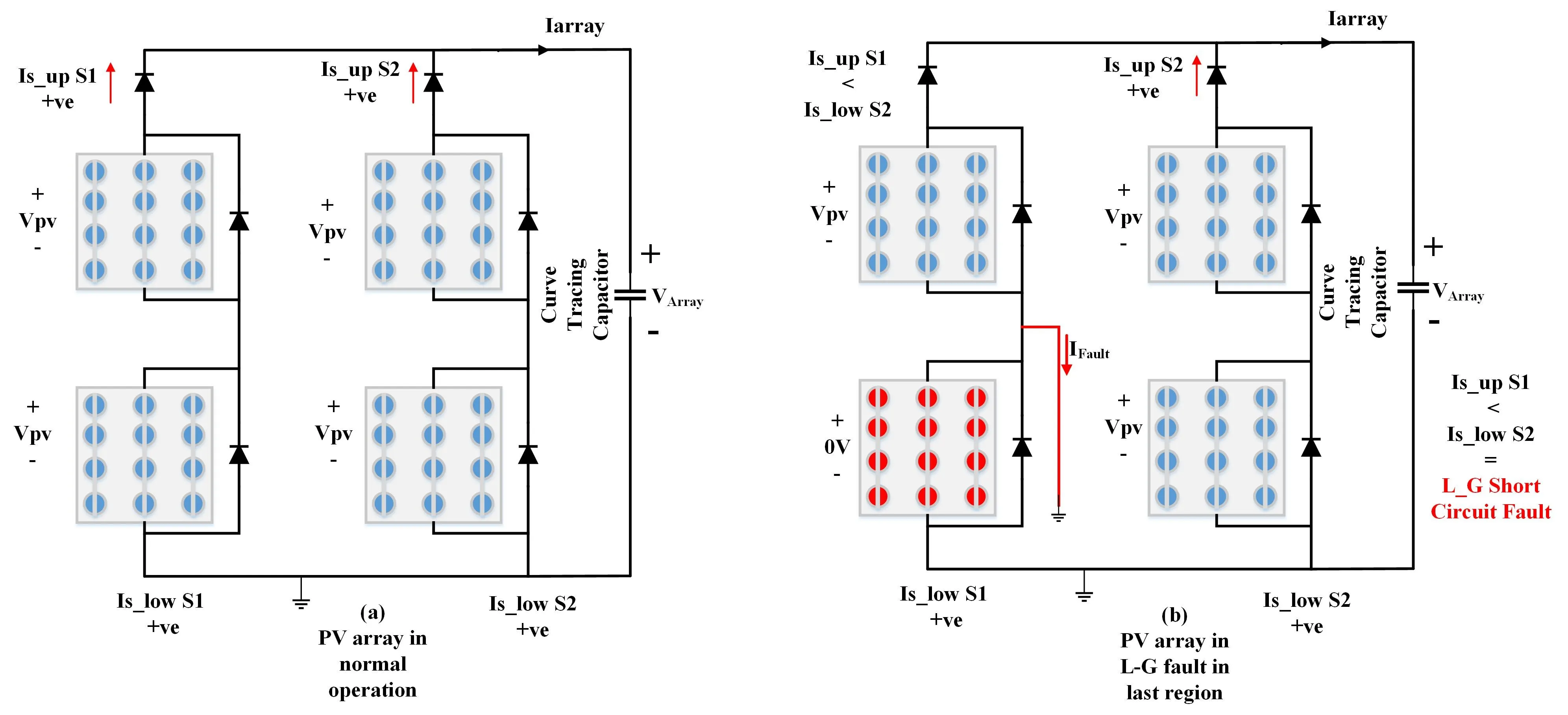
(1): L-G Fault

The two sensors’ data will be compared to detect which type of short circuit fault is present in our system, so that a sensing mechanism can be proposed. When an L-G fault occurs, the current in the PV strings will not follow its conventional path but will follow the short-circuit path. This is elaborated in Figure 3. Sensing signal: Is_up S1 < Is_low S2. Whenever this condition is satisfied, it will indicate that our system has encountered an L-G fault.

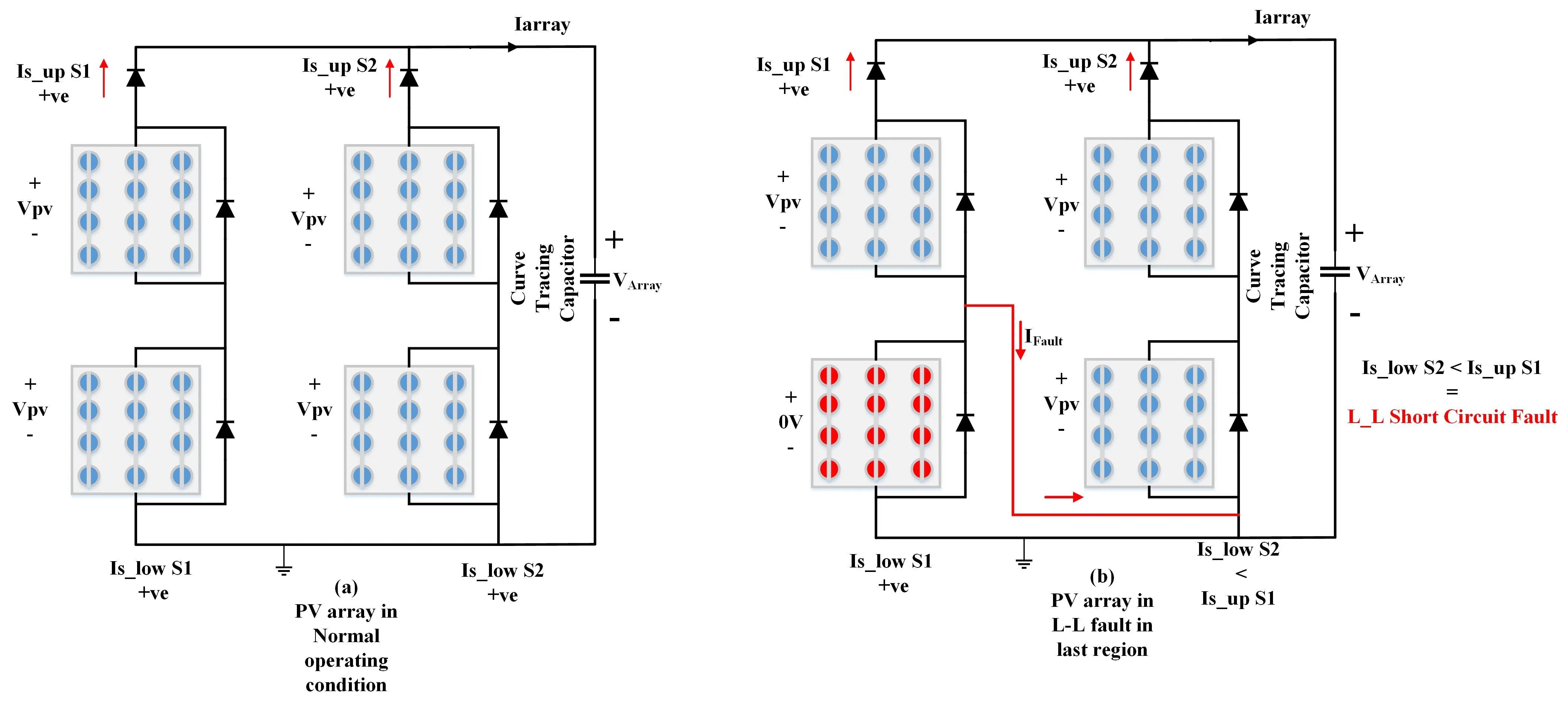
(2): L-L fault

Data from the two proposed current sensors will be evaluated and compared with each other. The L-L fault mechanism is slightly changed from that of L-G in that one string gets attached to the other to cause a short circuit fault. This can be seen in Figure 4. Sensing signal: Is_up S2 < Is_low S1. Whenever this condition is satisfied, it will indicate that our system has encountered an L-G fault.

Figure 3. (a) PV strings in normal condition. (b) PV strings with L-G fault.

Figure 4. (a) PV strings in normal condition. (b) PV strings with L-L fault.

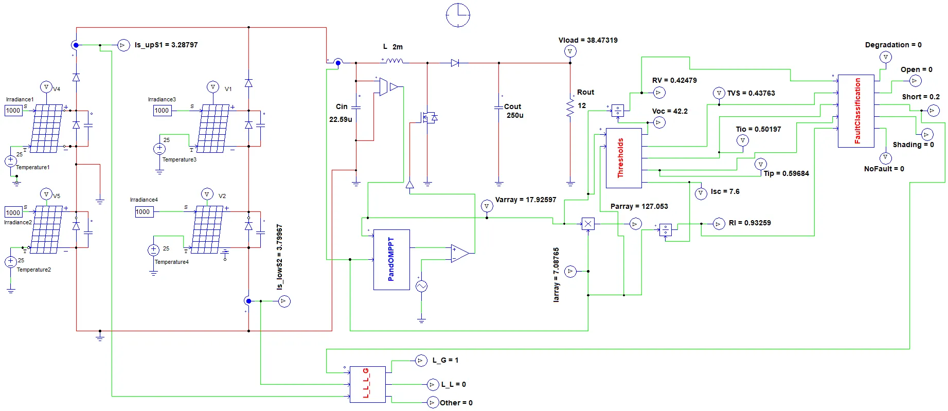
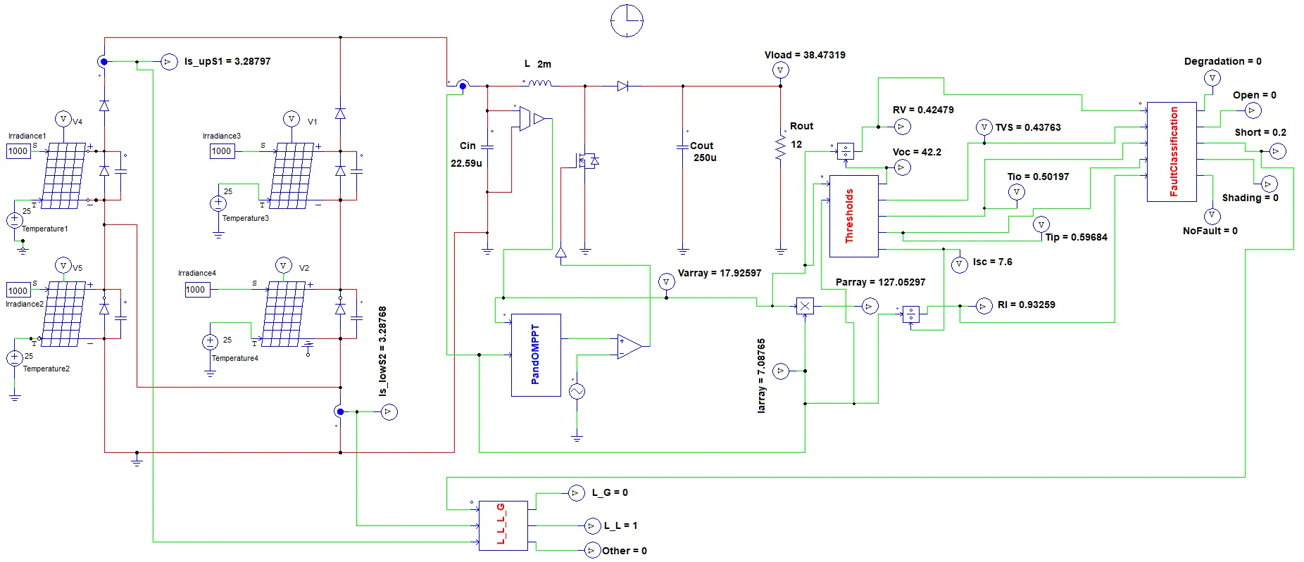
2.2. Proposed Fault Detection and Classification Circuit (FDCC) In Figure 5, the proposed fault detection and classification circuit is shown in the proposed circuit. There are four control blocks used in the sky blue block the MPPT (P&O) is running which will give a duty signal to the switching device present in the DC-DC converter. Each control block is in sync with each other.

Figure 5. The proposed fault detection and classification.

After this initial procedure, there comes a threshold block in yellow color, with the help of mathematical equations discussed in Section 2. Thresholds of four different types of faults are classified. Varray and I array are the inputs of this block. There will be 5 outputs of this block three of them are the thresholds for open circuit fault $$T_{I O}$$, shading fault $$T_{I P}$$, short circuit fault $$T_{V S}$$. The other two are $$V o c$$ and $$I s c$$ which are useful for the calculation of the current and voltage indicators $$\left( R_{I}\right), \left(R_{V}\right)$$. The five output signals of the threshold block are the input signals of the fault detection and classification (FDC). This block is mentioned in the circuit diagram in red color. In this block, a comparison of indicators with the thresholds is being done, and output signals of this block will detect and classify the faults. For the further classification of short circuit fault, another control block is used, which is in orange color. There are three inputs: two of the current sensors’ outputs and one is the short fault. In this block data from the current sensors is processed. If the FDC detects the presence of a short circuit fault, the L_G L_L classification block will start working, process the information, and classify which type of short fault is present in the system. 2.3. Flowchart of the Proposed HFDCA With the help of the conditions for the sensing signals in Table 1 and Table 2 for FDC, this flowchart of the proposed HFDCA. In Figure 6, the proposed hybrid fault detection and classification algorithm (HFDCA) is shown.

Table 1. Summary of Faults Sensing signal.

Fault Type	Sensing Signal
No fault	R_I > T_IO && R_V > T_VS
Degradation	R_I < T_IO && R_V < T_VS
Open	R_I < T_IO
Shading	R_I < T_IP
Short	R_V < T_VS

Table 2. Summary of Short Circuit Faults Sensing signal.

Fault Type	Sensing Signal
Short (L-G) Figure 3.	Is_up S1 < Is_low S2
Short (L-L) Figure 4.	Is_low S2 < Is_up S1

Figure 6. The proposed fault detection and classification algorithm flowchart.

The operation of this HFDCA is divided into three stages. In the first stage, the current and voltage indicators ratios will be defined alongside these thresholds will be created with the help of mathematical equations discussed earlier in Section 2 of this paper. In the second stage, the current and voltage indicator ratios are compared with the thresholds for each type of fault, and detection and classification will be done. In the third stage of this algorithm, the further classification of short circuit fault is being done. Here the algorithm will compare the data of two current sensors, one placed on the top of the first string and the second connected at the bottom of the second string. This placement of sensors can be seen in Fig By doing this, the algorithm will successfully detect and classify whether either system has an L-G or L-L short circuit fault.

3. Results and Discussion

All the previous discussions in Section 2 are verified with the help of a simulation of the proposed FDCC. The simulations are done on the PSIM 2022.1 Version. In Figure 7, the simulation setup for the proposed FDCC is presented. In the simulation circuit, four controllers are attached to the PV array. A boost converter is also installed in the proposed FDCC. The two current sensors are attached, and two displays are also attached for the measurement of current. Firstly, the MPPT (P&O) control block will give the Duty cycle to the mosfet used in the DC-DC Boost converter. Then, after this, a threshold control block is present, which will give 5 outputs for their values Five displays are attached with them that will display the threshold values and Voc and Isc. These parameters are discussed in Section 2 of this paper. For the detection and classification of faults, a controller is presented and five displays are attached. A value of 0.2 will be displayed on them according to the type of fault that occurs in the PVS. After this comes a control block that will detect and classify the L-G and L-L faults in the PVS. Three displays are attached to this block, and a value of 1 will be displayed on them according to the type of fault that occurred in the PVS. Specifications of the PV module and DC-DC boost converter are given below in Table 3 and Table 4.

Table 3. Specification of the PV module.

Maximum PV Module Power (Pm)	59.84 W
Open Circuit Voltage (Voc)	21.1 V
Short Circuit Current (Isc)	3.8 A
Max Current at MPP (I mpp)	3.5 A
Max Voltage at MPP (V mpp)	17.1 V

Table 4. Specification of boost converter.

Inductance (L)	2 mH
Capacitance (Cin)	22.59 uF
Capacitance (Cout)	250 uF
Resistive load (R)	12 ohms

Figure 7. Proposed 2X2 PV array schematic of FDCC.

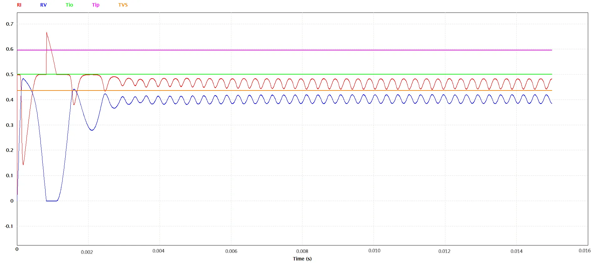
In the No-fault conditions, R_Iand R_Vare both greater than the fault thresholds T_IO, T_VS, and T_IP. This can be proved by Figure 8.

Figure 8. Current and voltage indicator ratios for no fault.

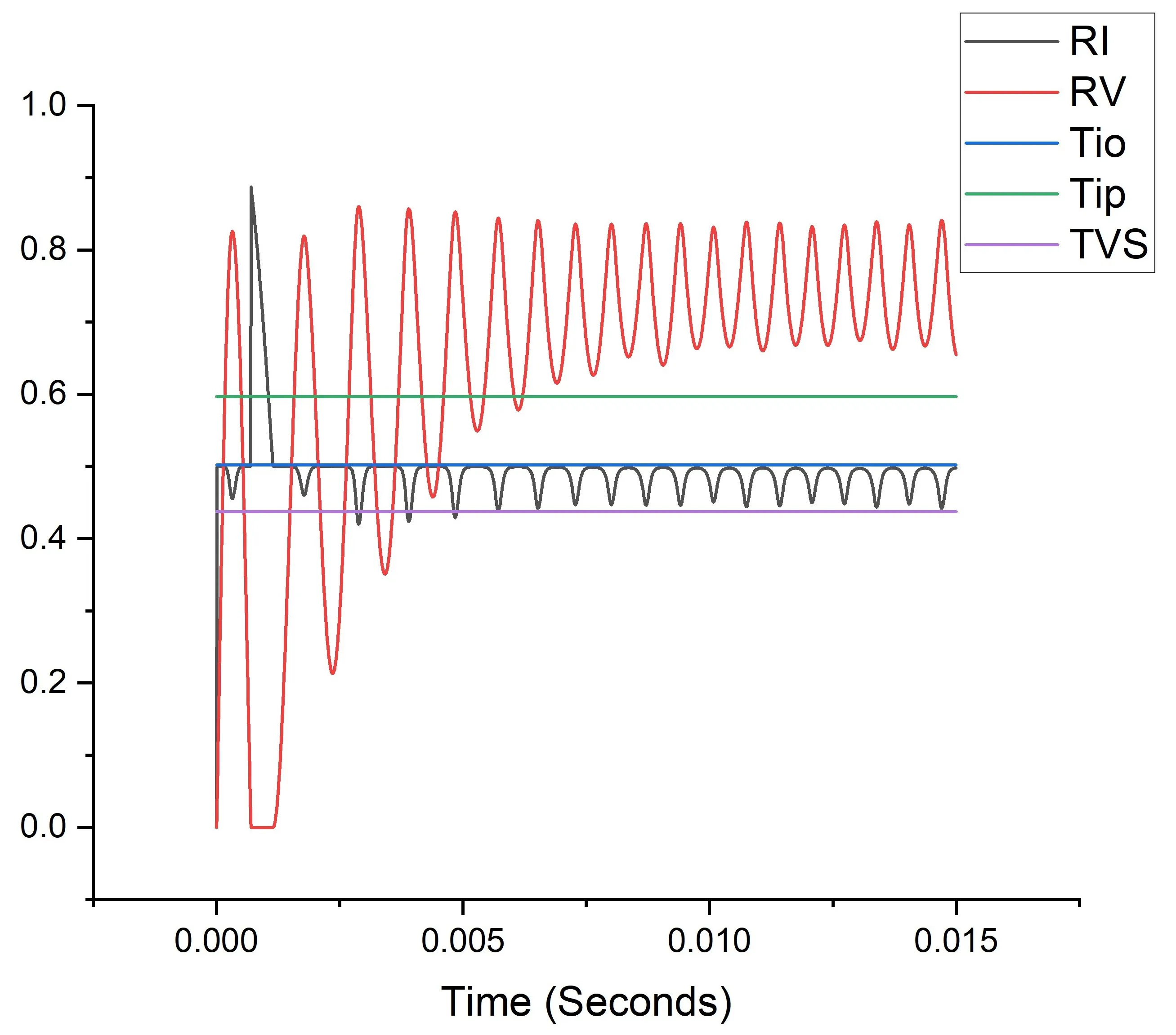
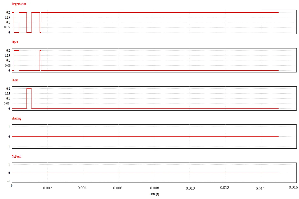
(A): Degradation:

As discussed in Section 2, whenever the current and voltage indicators are less than the open circuit fault threshold T_IO and short circuit fault threshold T_VS. In Figure 9. R_I = 0.48305 and R_V = 0.38573. Where T_IO = 0.50197 and T_VS = 0.43763. Hence, the sensing condition of Table 1 and 5 is satisfied, and the fault is classified as degradation. This is verified by a display named degradation in Figure 7, which will display 0.2 while other fault displays will give 0.

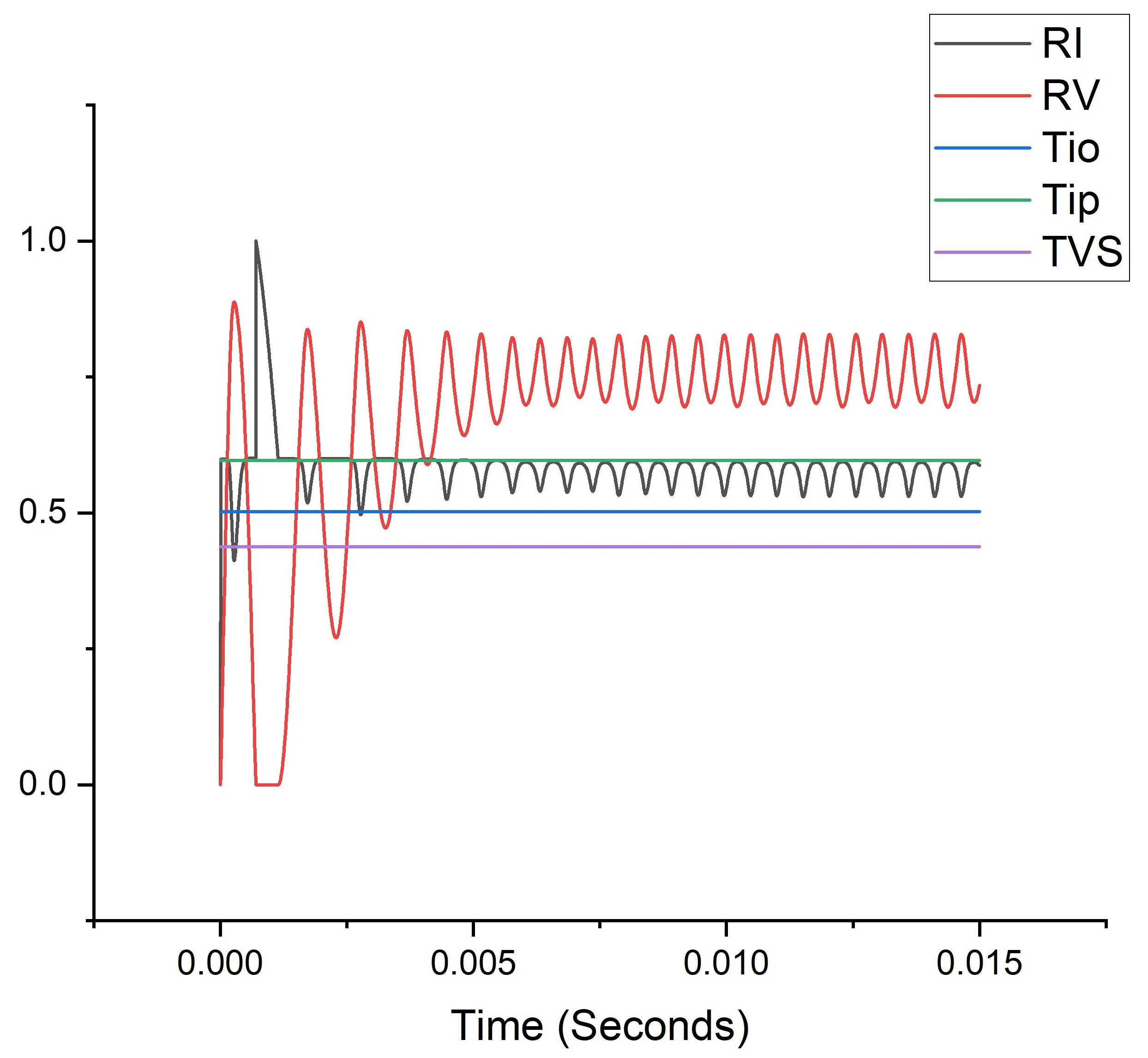
(B): Open Circuit Fault:

It is discussed in Section 2 that when the current indicator becomes less than the open circuit fault threshold, the algorithm in Figure will detect and classify the open circuit fault. In Figure 10. R_I = 0.49806 and T_IO = 0.50197, hence the sensing condition given in Table 1 and Table 5 is satisfied, and the given fault is classified as the open circuit fault. This detection and classification is verified by a display named Open in Figure 7, which will display 0.2 while other fault displays will give 0.

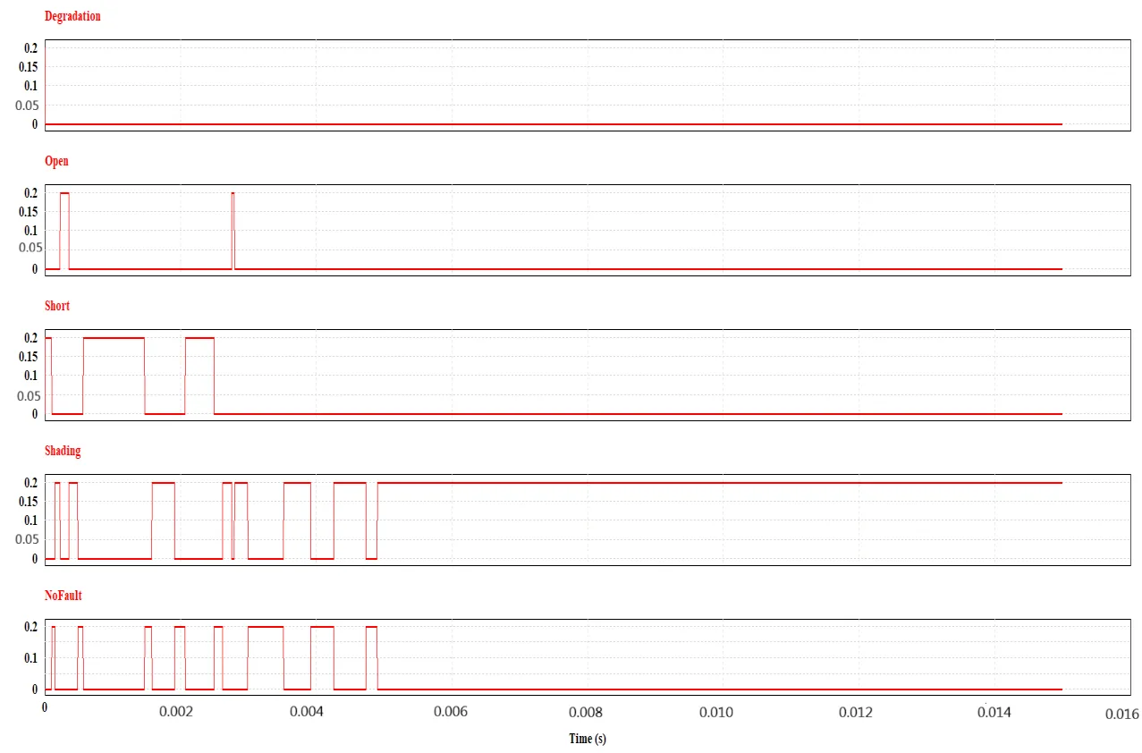
(C): Shading Fault:

Well, according to the discussion in Section 2. When a Shading fault occurs in PVS, the Current Indicator R_I becomes less than the shading fault threshold (T_IP). In Figure 11, R_I= 0.58727 and T_IP = 0.59684. Hence the sensing condition mentioned in Table 1 and Table 5 is satisfied and the fault is classified as a shading fault. This detection and classification is verified by a display named shading in Figure 7, which will display 0.2 while other fault displays will give 0.

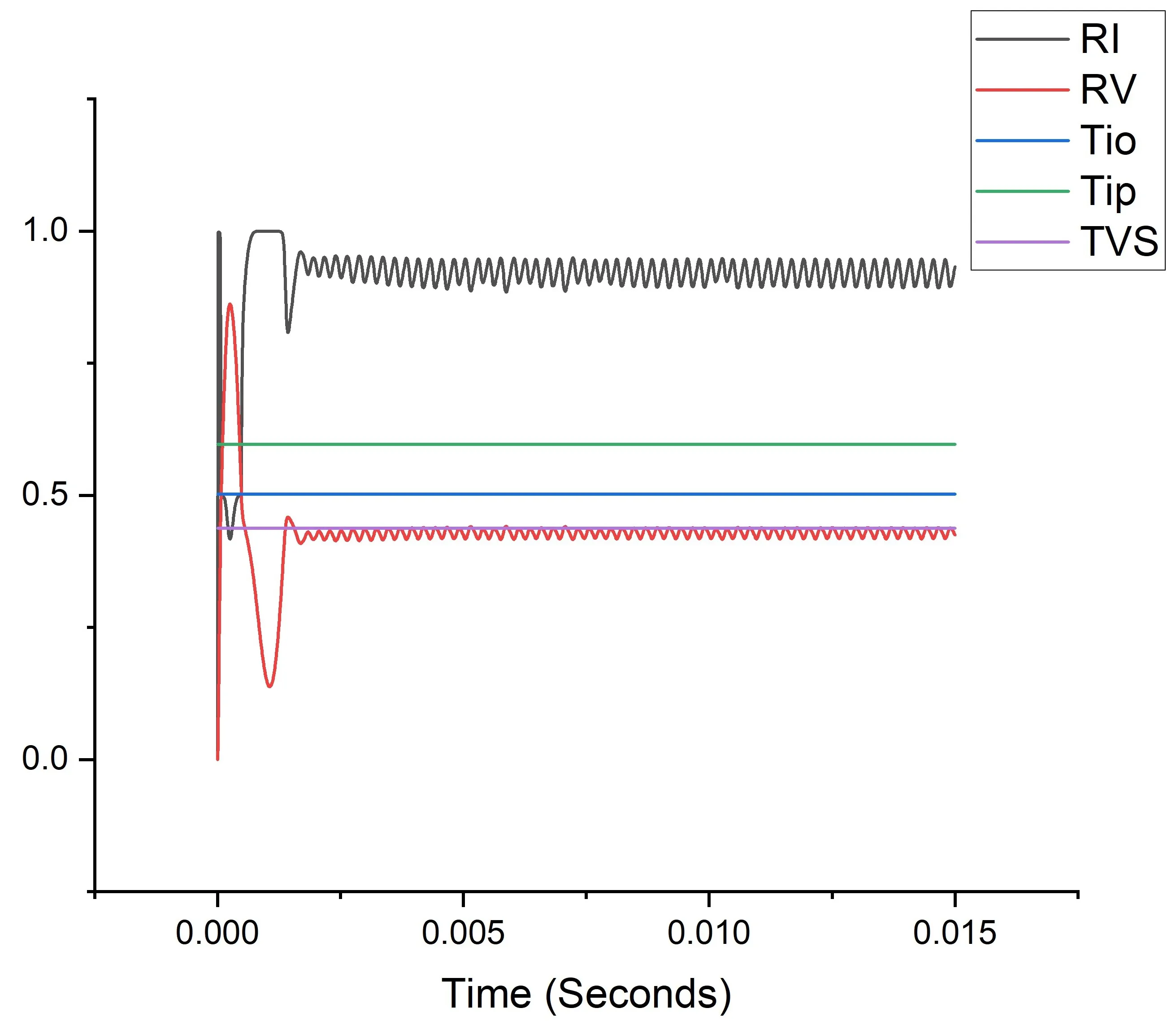
(D): Short circuit fault:

In Figure 12, the voltage indicator R_V = 0.42479 and the threshold T_VS = 0.43763. Hence, the sensing condition in Table 2 and 6 for the short circuit fault is satisfied. This detection and classification is verified by a display named short in Figure 7, which will display 0.2 while other fault displays will give 0. The simulation results of the displays classifying the above faults can be seen in Figure 13, Figure 14, Figure 15, Figure 16 and Figure 17.

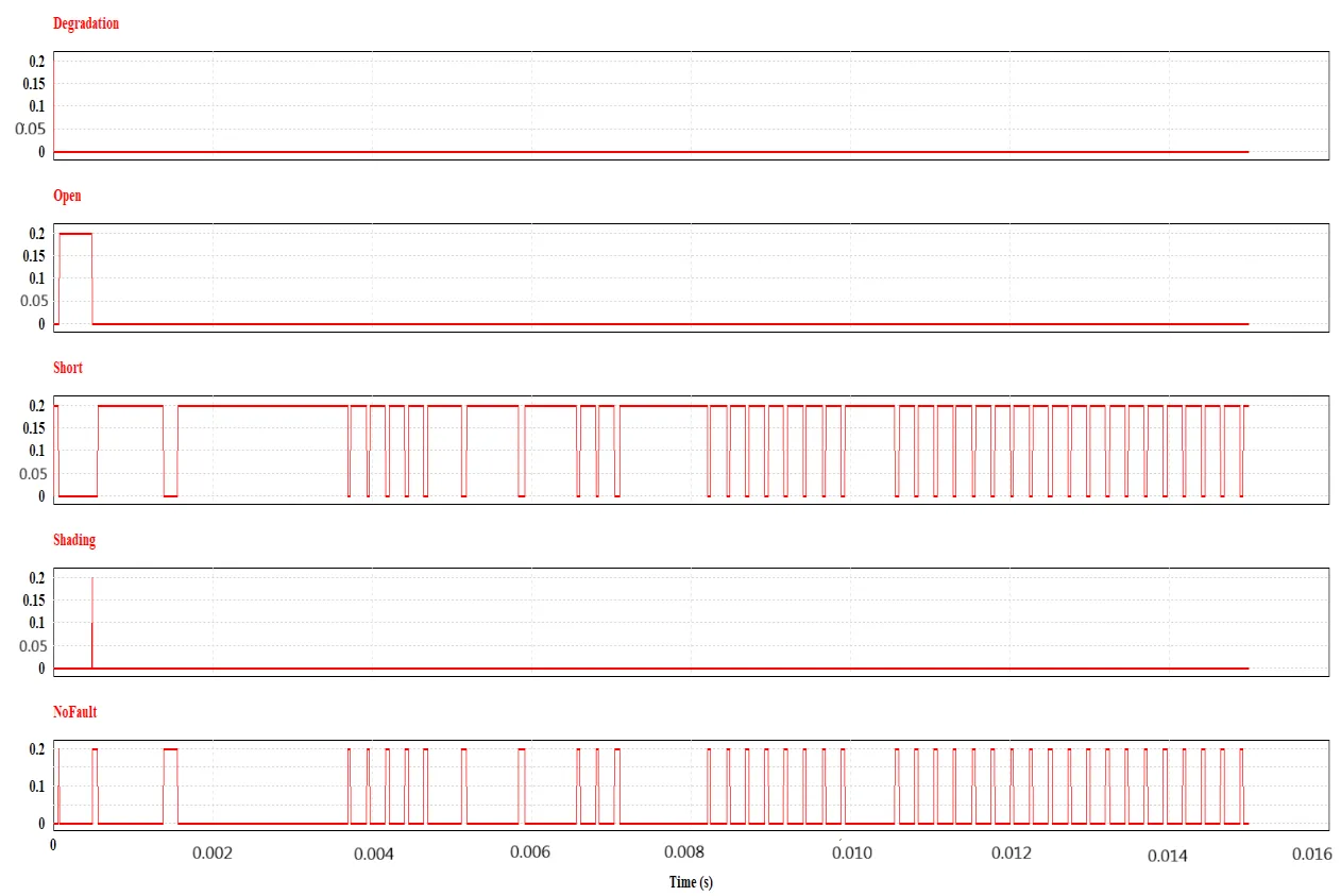
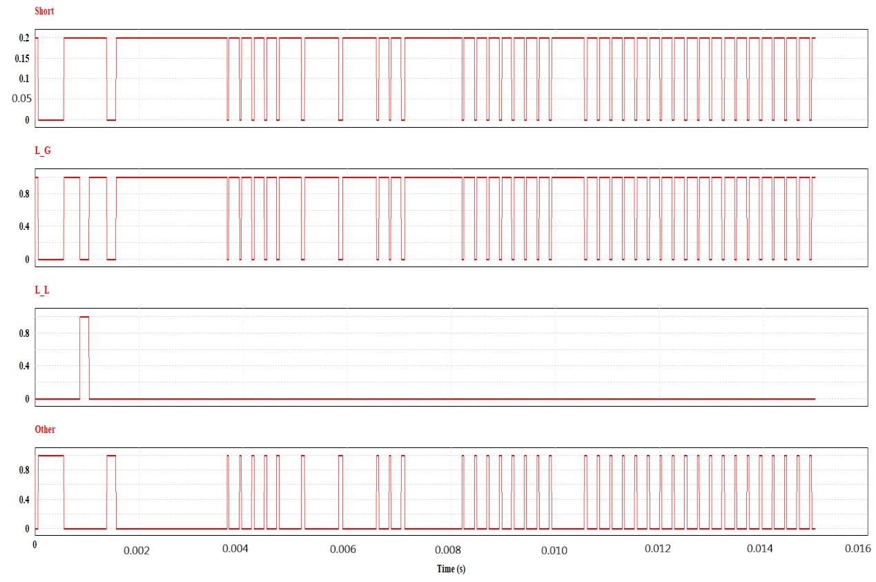
(1): L-G:

When the display named short gives a 0.2 value this will be the input of a block (L_L_L_G) for the further classification of the short circuit fault. In that block mentioned in Figure 7, the data from two current sensors Is_up S1 and Is_low S2 will be compared. In Figure 18, It is visible that the Is_up S1 = 3.28797 and Is_low S2 = 3.79967 which will satisfy the sensing condition of Table 2 and Table 6. The fault therefore, is classified as L-G fault and is verified by the display named L-G It will give 1 output value while other displays will show 0. This can also be verified by Figure 19.

(2): L-L:

When the display named short gives a 0.2 value, this will be the input of a block (L_L_L_G) for the further classification of the short circuit fault. In that block mentioned in Figure 7, the data from two current sensors Is_up S1 and Is_low S2 will be compared. In Figure 20. It is visible that the Is_up S1 = 3.28797 and Is_low S2 = 3.28768 which will satisfy the sensing condition of Table 2 and 6. The fault therefore, is classified as L-G fault and is verified by the display named L-G It will give 1 output value while other displays will show 0. This can also be verified by Figure 18.

Table 5. Summary of Faults Sensing signal.

	Current and Voltage Indicators		Thresholds
Fault Type	R_I	R_V	T_IO	T_VS	T_IP	Sensing Signal
No fault	0.96611	0.77146	0.50197	0.43763	0.59684	R_I > T_IO&& R_V > T_VS
Degradation	0.48305	0.38573	0.50197	0.43763	0.59684	R_I < T_IO&& R_V < T_VS
Open	0.49806	0.6549	0.50197	0.43763	0.59684	R_I < T_IO
Shading	0.58727	0.73496	0.50197	0.43763	0.59684	R_I < T_IP
Short	0.93259	0.42479	0.50197	0.43763	0.59684	R_V < T_VS

Table 6. Summary of Short Fault Sensing Signal.

	Current Sensors
Fault Type	String 1 (Is_up S1)	String 2 (Is_low S2)	Sensing Signal
Short (L-G) Figure 3.	3.28797 A	3.79967 A	Is_up S1 < Is_low S2
Short (L-L) Figure 4.	3.28797 A	3.28768 A	Is_low S2 < Is_up S1

Figure 9. Current and voltage indicator ratios for degradation.

Figure 10. Current and voltage indicator ratios for Open circuit fault.

Figure 11. Current and voltage indicator ratios for shading fault.

Figure 12. Current and voltage indicator ratios for Short circuit fault.

Figure 13. Degradation fault display result.

Figure 14. Open Circuit fault display result.

Figure 15. Shading fault display result.

Figure 16. Short circuit fault display result.

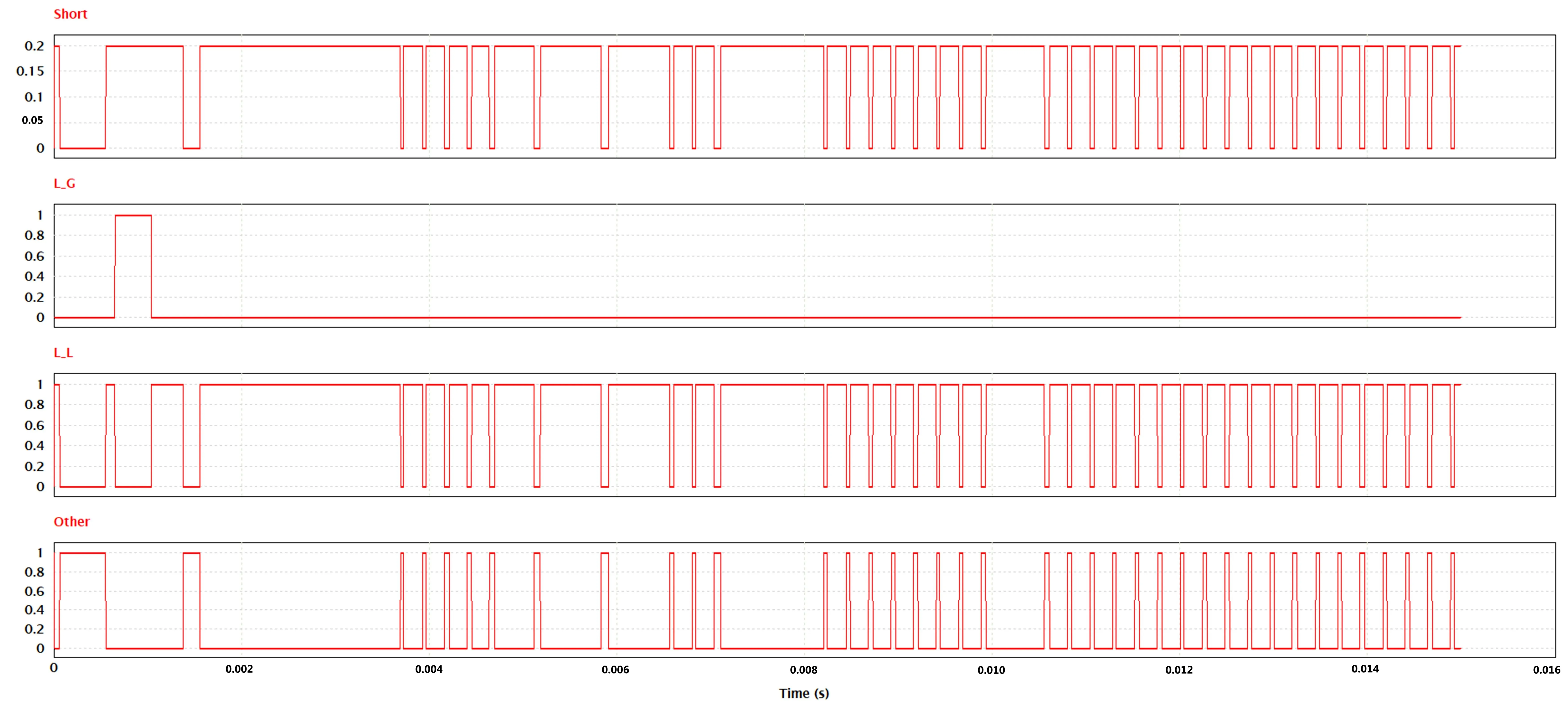
Figure 17. Short circuit (L-G) fault display result.

Figure 18. L_G fault Current sensor value.

Figure 19. Short circuit (L-L) fault display result.

Figure 20. L_L fault current sensor value.

4. Comparative Analysis

In [23], an algorithm detects and classifies L_L and L_G faults by utilizing two current sensors placed per string in a PV array. The only drawback of this technique is that it requires an additional number of sensors and extra channels on the microcontroller. Meanwhile, in [26], the algorithm can detect faults using mathematical equations and ratios. The drawback of this method is that it cannot distinguish between L_L and L_G faults. The proposed technique essentially accomplishes both by using a new hybrid algorithm that expands the range of faults detected and classified.

5. Conclusions

This research introduces a new hybrid fault detection and classification algorithm (HFDCA). It is concluded that faults are detected and classified through mathematical modeling and data from two current sensors. The algorithm effectively operates with blocking diodes in the PVS. Only two current sensors are required. This proposed FDCC and HFDCA offer a low-cost solution with no interfacing issues. The method successfully detects and classifies degradation, open circuit, shading, and short (L-G, L-L) faults. The algorithm only takes a few milliseconds to detect the faults.

Acknowledgments

The authors acknowledge technical support from the Punjab University in this project.

Author Contributions

Conceptualization, M.A.; Methodology, M.A.; Software, M.A.; Validation, M.A., K.H.; Formal Analysis, M.A.; Investigation, M.A.; Data Curation, M.A.; Writing—Original Draft Preparation, M.A., F.K., A.K.S.; Writing—Review & Editing, M.Q.S., R.Z.; Visualization, M.A., M.Q.S., M.B.S.; Supervision, K.H.; Project Administration, K.H.

Ethics Statement

Not applicable.

Informed Consent Statement

Not applicable.

Data Availability Statement

Funding

This research received no external funding.

Declaration of Competing Interest

The authors declare that they have no known competing financial interests or personal relationships that could have appeared to influence the work reported in this paper.

Nomenclature

PVS	Photovoltaic system
OCPD	Overcurrent protection
GCPD	Ground fault protection
V_oc	Open circuit voltage
I_sc	Short circuit current
G	Irradiation
T	Temperature
I_mpp	Maximum power point current
V_mpp	Maximum power point voltage
STC	Standard testing conditions
T_IO	open circuit fault threshold value
T_IP	Partial shading fault threshold value
T_VS	Short circuit fault threshold value
R_I	Current indicator
R_V	Voltage indicator
$$\bm{\epsilon}$$	Allowed offset value
V	Real-time voltage value
I	Real-time current value

References

Yi Z, Etemadi AH. Line-to-Line Fault Detection for Photovoltaic Arrays Based on Multiresolution Signal Decomposition and Two-Stage Support. IEEE Trans. Ind. Electron. 2017, 64, 8546–8556. [Google Scholar]

Hong YY, Pula RA. Methods of photovoltaic fault detection and classification: A review. Energy Rep. 2022, 8, 5898–5929. doi:10.1016/j.egyr.2022.04.043. [Google Scholar]

Triki-Lahiani A, Abdelghani AB, Slama-Belkhodja I. Fault detection and monitoring systems for photovoltaic installations: A review. Renew. Sustain. Energy Rev. 2018, 82, 2680–2692. [Google Scholar]

Dhimish M, Holmes V. Fault detection algorithm for grid-connected photovoltaic plants. Sol. Energy 2016, 137, 236–245. [Google Scholar]

Vergura S. Hypothesis Tests-Based Analysis for Anomaly Detection in Photovoltaic Systems in the Absence of Environmental Parameters. Energies 2018, 11, 485. [Google Scholar]

Chen L, Li S, Wang X. Quickest fault detection in photovoltaic systems. IEEE Trans. Smart Grid 2018, 9, 1835–1847. [Google Scholar]

Hariharan R, Chakkarapani M, Ilango GS, Nagamani C. A Method to Detect Photovoltaic Array Faults and Partial Shading in PVSystems. IEEE J. Photovolt. 2016, 6, 1278–1285. [Google Scholar]

Hu Y, Zhang J, Cao W, Wu J, Tian GY, Finney SJ, et al. Online Two-Section PV Array Fault Diagnosis with Optimized Voltage Sensor Locations. IEEE Trans. Ind. Electron. 2015, 62, 7237–7246. [Google Scholar]

Kumar BP, Ilango GS, Reddy MJ, Chilakapati N. Online Fault Detection and Diagnosis in Photovoltaic Systems Using Wavelet Packets. IEEE J. Photovolt. 2018, 8, 257–265. [Google Scholar]

10.

Yahyaoui I, Segatto ME. A practical technique for on-line monitoring of a photovoltaic plant connected to a single-phase grid. Energy Convers. Manag. 2017, 132, 198–206. [Google Scholar]

11.

Zhao Y, Ball R, Mosesian J, de Palma JF, Lehman B. Graph-based Semi-supervised Learning for Fault Detection and Classification in Solar Photovoltaic Arrays. IEEE Trans. Power Electron. 2015, 30, 2848–2858. [Google Scholar]

12.

Zhao Y, Lehman B, Ball R, Mosesian J, de Palma JF. Outlier detection rules for fault detection in solar photovoltaic arrays. In Proceedings of the 2013 Twenty-Eighth Annual IEEE Applied Power Electronics Conference and Exposition (APEC), Long Beach, CA, USA, 17–21 March 2013; pp. 2913–2920.

13.

Zhao Y, Balboni F, Arnaud T, Mosesian J, Ball R, Lehman B. Fault experiments in a commercial-scale pv laboratory and fault detection using local outlier factor. In Proceedings of the 2014 IEEE 40th Photovoltaic Specialist Conference (PVSC), Denver, CO, USA, 8–13 June 2014; pp. 3398–3403.

14.

Yi Z, Etemadi AH. Fault detection for photovoltaic systems based on multi-resolution signal decomposition and fuzzy inference systems. IEEE Trans. Smart Grid 2016, 8, 1274–1283. [Google Scholar]

15.

Roy S, Alam MK, Khan F, Johnson J, Flicker J. An irradiance-independent, robust ground-fault detection scheme for pv arrays based on spread spectrum time-domain reflectometry (sstdr). IEEE Trans. Power Electron. 2017, 33, 7046–7057. [Google Scholar]

16.

Karmacharya IM, Gokaraju R. Fault location in ungrounded photovoltaic system using wavelets and ann. IEEE Trans. Power Deliv. 2017, 33, 549–559. [Google Scholar]

17.

Harrou F, Taghezouit B, Sun Y. Improved k nn-based monitoring schemes for detecting faults in pv systems. IEEE J. Photovolt. 2019, 9, 811–821. [Google Scholar]

18.

Pillai DS, Rajasekar N. A comprehensive review on protection challenges and fault diagnosis in PV systems. Renew. Sustain. Energy Rev. 2018, 91, 18–40. [Google Scholar]

19.

Hu Y, Cao W, Wu J, Ji B, Holliday D. Thermography-Based Virtual MPPT Scheme for Improving PV Energy Efficiency Under Partial Shading Conditions. IEEE Trans. Power Electron. 2014, 29, 5667–5672. [Google Scholar]

20.

Al-Sheikh H, Moubayed N. Fault detection and diagnosis of renewable energy systems: An overview. In Proceedings of the 2012 International Conference on Renewable Energies for Developing Countries (REDEC), Beirut, Lebanon, 28–29 November 2012; pp. 1–7.

21.

Pillai DS, Rajasekar N. An mppt-based sensorless line– line and line–ground fault detection technique for pv systems. IEEE Trans. Power Electron. 2018, 34, 8646–8659. [Google Scholar]

22.

Wang W, Liu AC, Chung HS, Lau RW, Zhang J, Lo AW. Fault diagnosis of photovoltaic panels using dynamic current–voltage characteristics. IEEE Trans. Power Electron. 2015, 31, 1588–1599. [Google Scholar]

23.

Murtaza AF, Bilal M, Ahmad R, Sher HA. A circuit analysis based fault finding algorithm for photovoltaic array under ll/lg faults. IEEE J. Emerg. Sel. Top. Power Electron. 2019, 8, 3067–3076. [Google Scholar]

24.

Saleh KA, Hooshyar A, El-Saadany EF, Zeineldin HH. Voltage-based protection scheme for faults within utility-scale photovoltaic arrays. IEEE Trans. Smart Grid 2017, 9, 4367–4382. [Google Scholar]

25.

Silvestre S, da Silva MA, Chouder A, Guasch D, Karatepe E. New procedure for fault detection in grid connected PV systems based on the evaluation of current and voltage indicators. Energy Convers. Manag. 2014, 86, 241–249. [Google Scholar]

26.

Pei T, Hao X. A fault detection method for photovoltaic systems based on voltage and current observation and evaluation. Energies 2019, 12, 1712. [Google Scholar]