1. Introduction
1.1. Background
Urbanisation has significantly disrupted natural hydrological processes. As cities expand, the widespread replacement of permeable ground with impervious surfaces like concrete, asphalt, and rooftops has reduced infiltration, increased runoff, and contributed to frequent urban flooding. Conventional drainage infrastructure—dominated by pipes, gutters, and detention basins—is increasingly unable to cope, particularly under the growing pressure of climate-induced extreme rainfall events [
1,
2].
In response, urban water management has evolved to embrace more sustainable and resilient approaches, including Water Sensitive Urban Design (WSUD), Low Impact Development (LID), and Green Infrastructure (GI). These frameworks promote onsite retention, filtration, and slow release of stormwater, aiming not only to reduce flood risks but also to improve water quality, ecological health, and urban liveability [
3,
4,
5].
Swales are shallow, vegetated channels that slow and filter runoff while reducing flow volumes, protecting waterways, and providing both drainage conveyance and pretreatment for other stormwater measures. Their capacity to reduce flow volume, mitigate peak discharges, and remove pollutants through sedimentation and biological uptake has been extensively documented [
6,
7,
8]. Depending on the site and design goals, several types of swales can be deployed, including grassed swales with turf cover, dry swales using engineered media and underdrains, and bioswales that integrate dense vegetation and bioretention features [
9].
Swales are also inherently modular and adaptable. In compact urban settings, they can be retrofitted into road medians, parking lots, or green corridors. In peri-urban and suburban environments, they often function as ecological buffers between developed areas and natural waterways. Their compatibility with other nature-based solutions—such as permeable pavements, rain gardens, and constructed wetlands—makes them key components in distributed stormwater treatment systems [
10].
The global appeal of swales is exemplified by China’s “sponge city” initiative, which promotes rainwater capture, reuse, and infiltration at the source. These systems are not only valued for their hydraulic performance but also for their role in cooling urban areas, creating habitats, and enhancing recreational spaces [
11].
Emerging technologies such as remote sensing, Internet of Things (IoT), and real-time hydrological monitoring are further improving the efficiency and maintainability of swales by enabling continuous performance tracking and adaptive management [
6].
Swales are increasingly recognised as tools for ecosystem-based adaptation (EbA), offering nature-based solutions to reduce climate-related vulnerabilities while supporting urban biodiversity, carbon sequestration, and public amenity [
1]. Despite these advantages, several challenges limit widespread adoption, including the lack of consistent design standards, insufficient lifecycle cost data, and limited tools for comparing swales to traditional infrastructure [
1,
11].
This study aims to address these gaps through a techno-economic evaluation of swales in the South Australian context, assessing performance under current and future climate conditions. The research explores pollutant removal efficiencies, lifecycle costs, climate resilience, and integration with smart technologies—offering insights to guide urban planners, engineers, and policymakers toward more sustainable stormwater infrastructure solutions.
1.2. Literature Review
Grass swales have emerged as a cost-effective and sustainable solution for stormwater management, offering significant benefits in controlling runoff volumes, reducing peak flow rates, and improving water quality [
12]. The effectiveness of grass swales, however, is influenced by numerous factors including soil composition, vegetation type, rainfall intensity, and swale design parameters.
Controlled laboratory experiments have shown that grass swales with inclined side slopes, particularly those with a 1:3 gradient, are more effective at reducing peak flow compared to flat-bottomed configurations, due to enhanced flow distribution and infiltration potential [
13]. Soil mixtures with a high proportion of coarse sand (60%) combined with vegetative soil (40%) were found to achieve optimal drainage performance because of increased hydraulic conductivity. In addition, pollutant removal efficiency has been shown to vary significantly with vegetation type and substrate composition, with reported reductions in total suspended solids (TSS) ranging from 34.09% to 89.90% and total nitrogen (TN) by as much as 56.71% [
14].
Areas with shallow groundwater present challenges for swale performance, particularly due to variability in infiltration rates and diminished overall infiltration capacity. Infiltration measurements have ranged from as low as 13 mm/h at swale bottoms to as high as 98 mm/h along the slopes, suggesting that point-based measurements may overestimate average infiltration performance across a swale profile [
15]. Structural enhancements, such as retrofitted swale outlet control weirs (SOCWs), have been shown to improve runoff volume retention and peak flow reduction, especially during smaller storm events [
16].
Swales located near roadways are also subject to environmental challenges, notably the accumulation of traffic-related heavy metals in the soil. Elevated concentrations of metals such as lead (Pb), measured at 71 mg/kg dry weight, have been detected in older swales exposed to high traffic volumes [
17]. While swales have demonstrated the capacity to immobilize metals through infiltration, prolonged use can lead to soil contamination, which may necessitate costly soil remediation or replacement over time [
18].
Climatic conditions significantly impact swale performance. Zaqout & Andradóttir (2021) observed substantial declines in peak flow attenuation in winter due to frost and snow conditions, underscoring the importance of effective drainage in cold climates [
19]. To enhance sediment and metal removal, design modifications such as lengthening the swale and adopting trapezoidal cross-sections have been recommended, particularly for small to medium storm events [
20].
Hydraulic performance assessments have validated the effectiveness of grass swales in tropical settings, confirming their role in mitigating flash floods and conveying runoff under intense rainfall conditions [
21]. Moreover, the use of stepped ecological grass swales has been linked to significantly greater pollutant removal than conventional designs, highlighting their suitability for urban stormwater treatment applications [
22].
Hydraulic modelling has played a key role in improving swale design and performance assessment. To address inaccuracies in flow predictions caused by infiltration, a modified form of Manning’s equation has been developed, accounting for reductions in surface flow due to infiltration losses under different inflow conditions [
23]. Complementing this, an integrated hydrological model has been proposed that captures the dynamic behavior of swales, supporting its application in practical stormwater planning and design scenarios [
24].
Accounting for the temporal variability of saturated hydraulic conductivity (Ks) is also essential in enhancing modelling reliability. A dynamic estimation method using the Ensemble Kalman Filter (EnKF) has been introduced to track changes in Ks over time, thereby improving the accuracy of hydrological simulations [
25]. In parallel, a Bayesian network approach has been applied to identify representative rainfall event series, which is vital for conducting robust long-term performance evaluations of swale systems [
26].
Infiltration dynamics remain a key area of focus. Full-scale testing has revealed substantial spatial variability in Ks values across swale profiles, underlining the limitations of relying on point measurements and the need for comprehensive field-based assessments during the design phase [
27]. Adaptive implementation strategies have also been recommended, considering vegetation resilience under climate stress, runoff management effectiveness, and pollutant removal efficiency as core design considerations [
28].
Beyond site-specific design considerations, recent hydrological research highlights the broader role of vegetated swales within flood management and climate resilience strategies. Comparative studies of urban drainage design underscore the sensitivity of system performance to accurate estimation of time of concentration (ToC), with under- or overestimation significantly altering peak flow predictions and flood hydrographs [
29]. This aligns with swale-focused research emphasizing the importance of realistic infiltration and flow routing parameters to avoid overdesign or underperformance in practice.
Swales also contribute to mitigating impacts from extreme weather events. For example, analyses of Mediterranean cyclones such as Medicane Ianos and Daniel illustrate how intense rainfall and flash flooding strain conventional drainage networks, reinforcing the value of distributed, nature-based systems for absorbing and slowing runoff [
30,
31]. Similar lessons emerge from flood-induced hydro chemical changes in sensitive lagoons, where heavy rainfall events rapidly alter water quality, but systems with enhanced flushing and infiltration show resilience [
32]. These findings suggest that well-designed swales not only support urban runoff treatment but can also buffer downstream ecosystems from episodic pollutant loads.
Hydrological–hydraulic modelling further demonstrates the capacity of nature-based solutions, including swales, bioswales, and rain gardens, to reduce flood peaks and pollutant transport at the catchment scale [
33]. Such models stress the importance of embedding swales within integrated stormwater systems, where their modularity allows cost-effective retrofitting into diverse urban contexts. Incorporating satellite precipitation products and real-time monitoring enhances the accuracy of design rainfall inputs and supports adaptive management under climate variability [
31].
Collectively, these studies underscore the multifaceted role of grass swales in sustainable urban stormwater management, while situating them within the wider discourse on climate adaptation, catchment-scale hydrology, and resilience to extreme flood events. These insights reinforce the case for swales as versatile and economically viable stormwater infrastructure components, especially when supported by robust hydrological modelling and long-term monitoring.
2. Materials and Methods
This study adopted a systematic methodology to evaluate the performance and feasibility of vegetated swales for urban stormwater management in a semi-arid context. The approach integrated hydrologic and hydraulic analysis, conceptual swale design, pollutant treatment modelling, economic evaluation, and climate scenario testing. Each stage was grounded in established urban stormwater design practices and supported by site-specific data. The following subsections detail the study area, sub catchment delineation, flow estimation procedures, swale design criteria, MUSICX modelling configuration, lifecycle cost analysis, and adjustments made to account for future climate projections.
2.1. Study Area
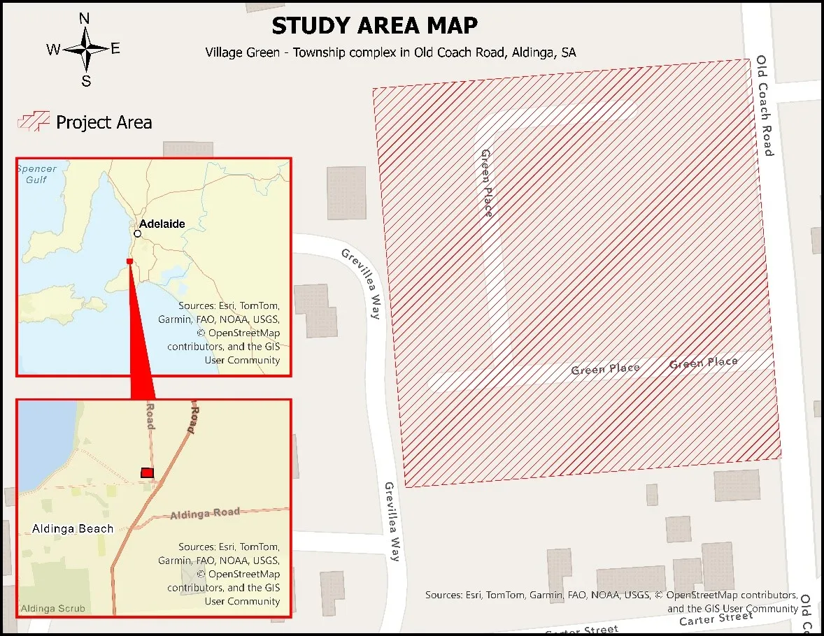
The study area is in Aldinga, a peri-urban township in South Australia, within the jurisdiction of the city of Onkaparinga as shown in . The site features sandy clay soils, mild slopes (1–4%), and increasing imperviousness due to residential development. The Village Green subdivision, a planned residential community, was selected as the focus area due to its representativeness of growth areas in semi-arid regions. The climate is Mediterranean, with hot dry summers and cool wet winters, making the site relevant for testing climate-resilient green infrastructure.
. Study area location map.
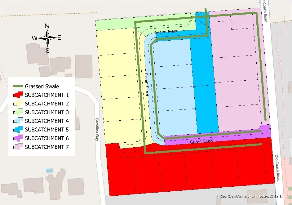
Subdivision plans and aerial imagery were used to delineate sub catchments corresponding to road and lot layouts as shown in .
. Sub catchments of the study area indicating location and distribution and of grassy swales.
Each sub catchment was characterized based on:
-
-
Land use composition (e.g., roadway, residential allotments, open space)
-
-
Impervious area ratio
-
-
Average slope and flow length
-
-
Drainage flow paths
-
-
Sub catchment boundaries were digitized using AutoCAD.
To accurately assess the impervious contribution from each land use type, the following assumptions were applied in line with established hydrological design guidelines:
-
-
Residential areas: Assumed to be 70% impervious, accounting for rooftops, driveways, and paved surfaces. This reflects a probable maximum development condition typical in medium-density subdivisions [34].
-
-
Road areas: Considered 100% impervious due to continuous asphalt or concrete surfacing [35].
To support hydrologic modelling, seven sub catchments were delineated within the Village Green development using subdivision layout plans. The impervious area estimates were based on aerial imagery interpretation and design assumptions aligned with ARR [
34]. The summary of area distribution is provided in
.
.
Sub catchment properties (pervious and impervious areas within each sub catchment).
| Sub Catchment No. |
Total Area (m2) |
% of Impervious Area |
% of Pervious Area |
| 1 |
4833.22 |
65.215% |
34.785% |
| 2 |
3616.29 |
65.305% |
34.695% |
| 3 |
1085.12 |
24.868% |
75.132% |
| 4 |
2997.87 |
66.078% |
33.922% |
| 5 |
1654.15 |
65.709% |
34.291% |
| 6 |
597.70 |
47.020% |
52.980% |
| 7 |
3426.55 |
66.929% |
33.071% |
| Total |
18,210.90 |
62.741% |
37.259% |
These values informed the calculation of composite runoff coefficients, time of concentration, and rainfall intensity for each sub catchment. These parameters were subsequently used in the rational method to estimate peak flows and guide swale design.
2.3. Determination of Design Flow
2.3.1. Runoff Coefficient
To reflect the range of storm events considered in this study, runoff coefficients were determined for both the 1-year and 100-year Average Recurrence Intervals (ARI). The base runoff coefficients (
C10) for a 10-year ARI were taken as 0.10 for pervious areas and 0.90 for paved (impervious) surfaces. These were adjusted using the recommended frequency factors as shown in
[
35].
.
Frequency conversion factors.
| ARI (Years) |
1 |
2 |
5 |
10 |
20 |
40 |
60 |
80 |
100 |
| F |
0.8 |
0.85 |
0.95 |
1.00 |
1.05 |
1.13 |
1.17 |
1.19 |
1.20 |
The runoff coefficients (
C1, and
C100) were determined using the equation:
where:
Cy represents the effective runoff coefficient for the
y-year ARI;
Fy is the frequency factor for the
y-year ARI, and
C10 is the basic runoff coefficient for a 10-year ARI.
For the 1-year ARI, relevant to the design of the swales under typical operational conditions, a factor (
F1) of 0.80 was applied, resulting in adjusted coefficients of 0.08 for pervious areas and 0.72 for paved surfaces. For the 100-year ARI, which was used to evaluate the potential for overflow during extreme storm events, a factor (
F100) of 1.20 was used. This yielded coefficients of 0.12 for pervious areas and 1.08 for paved surfaces; the latter was capped at applied 1.00 to comply with hydrologic modelling standards.
These ARI-specific values were then used in a weighted average method to calculate the effective runoff coefficient for each sub catchment, given by the equation:
The ARI-specific runoff coefficients are given in
. The 1-year ARI coefficients informed the swale design to handle routine stormwater runoff effectively, while the 100-year ARI coefficients were used to test the system’s resilience and ensure that overflow risks were minimized during rare but intense storm events.
.
Effective runoff coefficients (C1 and C100) of each sub catchment.
| Sub-Catchment No. |
Area Pervious |
Area Impervious |
Total Area (m2) |
C1 |
C100 |
| 1 |
1681.26 |
3151.96 |
4833.22 |
0.4974 |
0.6939 |
| 2 |
1254.66 |
2361.63 |
3616.29 |
0.4980 |
0.6947 |
| 3 |
815.27 |
269.85 |
1085.12 |
0.2392 |
0.3388 |
| 4 |
1016.93 |
1980.94 |
2997.87 |
0.5029 |
0.7015 |
| 5 |
567.23 |
1086.92 |
1654.15 |
0.5005 |
0.6982 |
| 6 |
316.66 |
281.04 |
597.70 |
0.3809 |
0.5338 |
| 7 |
1133.19 |
2293.37 |
3426.55 |
0.5083 |
0.7090 |
2.3.2. Time of Concentration
The time of concentration (
tc), defined as the time it takes for runoff from the most distant point of a sub catchment to reach the outlet. Consistent with guidance provided in Australian Rainfall and Runoff (2019), tc was estimated using Probabilistic Rational Method (PRM) equation [
34]:
where
tc is in hours and
A is the sub catchment area in km
2. This equation is consistent with urban stormwater design practice and allows for a simplified estimation of flow response time based on catchment size.
To complement the use of the PRM above, the Haktanir & Sezen (HS) (1990) empirical formula for estimating time of concentration (
tc)was also considered. This method is particularly relevant in cases where only the main channel length (
Lc) is available, as it defines
tc (hours) as:
where
Lc is the channel length in kilometres. Unlike area-based relations, the HS equation relies solely on flow path length, making it practical for small catchments such as the Village Green development in Aldinga where slope information was not available.
The resulting values from the PRM ranged from approximately 2.7 to 6.0 min across the seven delineated sub catchments, with smaller areas producing shorter response times. In comparison, the HS method yielded consistently higher values, between 6.2 and 8.1 min, reflecting the stronger influence of channel length on travel time.
presents the total area of each sub catchment along with the computed
tc values in both hours and min.
.
Total area of each sub catchment with corresponding tc values in hours and min.
| Sub-Catchment No. |
Total Area (km2) |
tc (PRM) (h) |
Tc (PRM) (min) |
Tc (HS) (h) |
Tc (HS) (min) |
| 1 |
0.0048 |
0.1001 |
6.0000 |
0.1350 |
8.1000 |
| 2 |
0.0036 |
0.0897 |
5.3800 |
0.1217 |
7.3000 |
| 3 |
0.0011 |
0.0567 |
3.4000 |
0.1029 |
6.1700 |
| 4 |
0.0030 |
0.0835 |
5.0100 |
0.1059 |
6.3500 |
| 5 |
0.0017 |
0.0666 |
3.9900 |
0.1159 |
6.9500 |
| 6 |
0.0006 |
0.0452 |
2.7100 |
0.1069 |
6.4100 |
| 7 |
0.0034 |
0.0879 |
5.2700 |
0.1294 |
7.7600 |
These
tc values were used to determine the critical rainfall intensity corresponding to each sub catchment using Intensity–Duration–Frequency (IDF) data. These intensities, in turn, formed part of the Rational Method for computing peak discharge, which guided the design of the swales.
2.3.3. Intensity–Frequency–Duration (IFD) Relationships
Intensity–Frequency–Duration (IFD) relationships describe how rainfall intensity varies with storm duration and recurrence probability. For this study, location-specific IFD values were obtained directly from the Australian Bureau of Meteorology’s (BoM) online IFD 2016 data system, which provides calibrated design rainfall estimates derived from long-term gauge records and regional climatic conditions across South Australia (Bureau of Meteorology, Adelaide, South Australia, 2016). The BoM system supplies rainfall depths for selected durations and annual exceedance probabilities (AEPs), which are converted to intensities using the fundamental relationship (Bureau of Meteorology, 2016):
Rainfall intensities for each sub catchment were determined based on the computed time of concentration (
tc), using IFD data corresponding to the coordinates of the Village Green residential subdivision in Aldinga (Latitude: –35.265°, Longitude: 138.482°) [36]. Table 5 presents the extracted data corresponding to durations nearest to the calculated
tc values.
.
IFD values for Village Green residential development area extracted from BoM IFD online portal.
| Duration in min |
I (ARI = 1) |
I (ARI = 100) |
| 2 |
69.0 |
218.0 |
| 3 |
61.1 |
195.0 |
| 4 |
54.9 |
177.0 |
| 5 |
50.1 |
163.0 |
| 10 |
36.0 |
119.0 |
Vegetated swales in this study were designed for typical storm events using the 1-year ARI as the primary design parameter, consistent with the WSUD Technical Manual for Greater Adelaide which recommends targeting frequent, small events for water quality treatment. To assess resilience, system performance was also tested against the 100-year ARI to evaluate conveyance capacity and overflow risk.
Extreme rainfall—and therefore flood risk—in Australia is projected to increase, requiring design rainfalls from the 2016 IFDs to be adjusted using a temperature-scaling approach consistent with IPCC projections to reflect rising global temperatures since the 1961–1990 baseline [
34].
Rainfall intensities were adjusted for medium-term climate scenario under RCP8.5 as shown in
. The adjustments were computed using the equation:
where:
Ip the projected (current or future) design rainfall depth or intensity;
α is the rate of change;
I is the historical design rainfall depth or intensity from the 2016 IFD portal; Δ
T is the most up-to-date estimate of global (land and ocean) temperature projection for the design period of interest and selected climate scenario relative to a baseline period.
.
Medium-term adjusted rainfall intensities under RCP 8.5.
| Duration in min |
I (ARI = 1) |
I (ARI = 100) |
| 2 |
92.54 |
292.36 |
| 3 |
81.94 |
261.52 |
| 4 |
67.19 |
237.38 |
| 5 |
54.90 |
218.60 |
| 10 |
48.28 |
159.59 |
Rainfall intensities were interpolated from IFD curves based on each subcatchment’s
tc, which ranged from approximately 2.7 to 6.0 min. For the 1-year ARI (
I1), intensities varied from 63.4 mm/h to 84.9 mm/h. The highest intensity was observed for Sub catchment 6 due to its short
tc of 2.72 min, indicating a fast hydrological response and thus requiring careful design consideration. Conversely, Sub catchment 1 had the lowest
I1 value, corresponding to its longer
tc of 6.01 min. Under the 100-year ARI (
I100), the intensities ranged from 206.7 mm/h to 270.3 mm/h, following a similar pattern where shorter
tc values resulted in higher intensity estimates.
These interpolated intensities were used alongside the effective runoff coefficients in the Rational Method to estimate peak discharge rates for both routine and extreme storm scenarios, thereby supporting swale design and overflow risk assessment. A summary of the
tc values and associated rainfall intensities is presented in
.
.
Interpolated rainfall intensity values corresponding to ARI = 1 and ARI = 100.
| Sub-Catchment No. |
tc (mins) |
I1 (PRM) |
I100 (PRM) |
I1 (HS) |
I100 (HS) |
| 1 |
6.0114 |
63.365 |
206.665 |
63.408 |
206.800 |
| 2 |
5.3840 |
65.738 |
214.070 |
65.753 |
214.117 |
| 3 |
3.4076 |
78.553 |
251.678 |
73.241 |
237.484 |
| 4 |
5.0136 |
67.138 |
212.908 |
67.152 |
218.483 |
| 5 |
3.9997 |
73.630 |
237.385 |
71.010 |
230.521 |
| 6 |
2.7166 |
84.944 |
270.258 |
75.850 |
245.628 |
| 7 |
5.2749 |
66.150 |
215.358 |
66.169 |
215.415 |
2.4. Design Flow Computation
The peak flow rate (
Q) for each sub catchment was calculated using the Rational Method, expressed as:
where:
Q is the peak flow rate in cubic meters per second (m
3/s),
C is the effective runoff coefficient (dimensionless),
I is the rainfall intensity in millimeters per hour (mm/h), and A is the catchment area in hectares (ha).
This method provides a straightforward means of estimating peak discharge during storm events based on sub catchment hydrology and local rainfall conditions. For this study,
I was taken from interpolated IFD data for both the 1-year and 100-year ARIs,
A was determined from the area characterization of each sub catchment using AutoCAD, and
C was calculated using a weighted average of pervious and impervious areas. The resulting peak flows were used to size the swale infrastructure under design conditions and evaluate performance under extreme events. The calculated values for each sub catchment are presented in
.
.
Computed peak discharges (Q) for sub-catchments 1–7 under 1-year and 100-year ARI events using the Probabilistic Rational Method (PRM) and Haktanir & Sezen (HS) algorithms.
| Sub-Catchment No. |
C1 |
C100 |
A (ha) |
Q1 (PRM) (m3/s) |
Q100 (PRM) (m3/s) |
Q1 (HS) (m3/s) |
Q100 (HS) (m3/s) |
| 1 |
0.4974 |
0.6939 |
0.4833 |
0.042 |
0.193 |
0.042 |
0.193 |
| 2 |
0.4980 |
0.6947 |
0.3616 |
0.033 |
0.149 |
0.033 |
0.149 |
| 3 |
0.2392 |
0.3388 |
0.1085 |
0.006 |
0.026 |
0.005 |
0.024 |
| 4 |
0.5029 |
0.7015 |
0.2998 |
0.028 |
0.124 |
0.028 |
0.128 |
| 5 |
0.5005 |
0.6982 |
0.1654 |
0.017 |
0.076 |
0.016 |
0.074 |
| 6 |
0.3809 |
0.5338 |
0.0598 |
0.005 |
0.024 |
0.005 |
0.022 |
| 7 |
0.5083 |
0.7090 |
0.3427 |
0.032 |
0.145 |
0.032 |
0.145 |
The computed peak discharges (
Q) for the seven delineated sub-catchments highlight the sensitivity of results to the choice of time of concentration algorithm. Using the Probabilistic Rational Method (PRM), estimated
Q1 values (1-year ARI) ranged from 0.005 to 0.042 m
3/s, while
Q100 values (100-year ARI) ranged from 0.024 to 0.193 m
3/s. In contrast, the Haktanir & Sezen (HS) (1990) method produced nearly identical discharge values for each sub-catchment, differing only marginally from those obtained using PRM.
This similarity occurs because both methods yield Tc values within the same order of magnitude (generally between 3 and 8 min), which correspond to short rainfall durations on the intensity–duration–frequency (IDF) curves. As a result, the selected rainfall intensities for the two Tc sets are close, leading to only minor differences in
Q. The small discrepancies that do appear, for example, in Sub-catchments 3 and 5, reflect the slightly longer Tc values from the Haktanir & Sezen formula, which reduce the rainfall intensity and consequently the calculated discharge.
Overall, the comparison demonstrates that for very small catchments (≤0.005 km
2) in South Australian rural developments, the choice between PRM and HS has little effect on peak discharge outcomes, particularly at lower ARIs.
2.5. Manual Swale Design
Swale geometry was manually designed to accommodate the peak flow rates computed for each sub catchment. Standard trapezoidal cross-sections were adopted, with side slopes set at 1V:3H, in line with Water Sensitive Urban Design (WSUD) guidelines. This configuration provided an effective balance between hydraulic performance, erosion control, and ease of maintenance. To determine the required dimensions, Manning’s equation was used to calculate the necessary cross-sectional area and shape that would convey the design flow within the available space:
where
Q is the design flow (m
3/s),
A is the cross-sectional area (m
2),
R is the hydraulic radius (m),
S′ is the channel slope, and
n is the Manning’s roughness coefficient. The hydraulic radius
R is defined as the ratio of the cross-sectional area to the wetted perimeter (
R =
A/
P).
Following the hydraulic design process using Manning’s equation, swale dimensions were finalized for each of the seven sub catchments. The design flows derived from both the Probabilistic Rational Method (PRM) and the Haktanir & Sezen (1990) equation were used to size the swales. As expected, the small differences in peak discharge between the two Tc formulations resulted in only minor variations in the computed cross-sections. In all cases, the prescribed 1V:3H side slopes were maintained, and top widths were checked to ensure compliance with the maximum constraint imposed by the site layout.
As shown in
, Manual swale design dimensions., base widths ranged from 0.5 to 2.0 m and depths from 0.15 to 0.40 m, while the resulting top widths varied between 1.4 and 4.4 m depending on hydraulic capacity requirements. Swale lengths were governed by grading and alignment considerations, with values between 56 and 114 m. Although the Haktanir & Sezen method consistently produced slightly lower peak discharges due to its longer Tc estimates, the differences were not large enough to change the overall design envelope. The final swale dimensions were unchanged across both Tc estimation methods, indicating that the choice of algorithm had no material influence on the design outcomes.
.
Manual swale design dimensions.
| Swale |
Length |
Depth |
Base Width |
Top Width |
| S1 |
114.0000 |
0.3500 |
1.4000 |
3.500 |
| S2 |
90.0000 |
0.4000 |
1.4000 |
3.800 |
| S3 |
77.0000 |
0.4000 |
2.0000 |
4.400 |
| S4 |
76.0000 |
0.1500 |
0.5000 |
1.400 |
| S5 |
56.0000 |
0.2500 |
0.8000 |
2.300 |
| S6 |
79.0000 |
0.3000 |
1.1000 |
2.900 |
| S7 |
95.0000 |
0.3000 |
0.9000 |
2.700 |
This outcome highlights an important practical implication: although different empirical formulas for Tc produced slightly different numerical values, these differences did not alter the final swale dimensions. For very small catchments in South Australian rural developments, the comparison confirms that swale sizing is effectively insensitive to the choice of Tc algorithm. This strengthens the analysis by demonstrating that the hydraulic design remains consistent regardless of the method applied.
2.6. MUSICX Model and Simulation
2.6.1. Meteorological Data Input
The MUSICX model was run using built-in rainfall data from the year 1970, which includes daily rainfall and potential evapotranspiration (PET) values. This dataset was cross-checked against Bureau of Meteorology (BoM) records from the five nearest stations using Inverse Distance Weighing and was found appropriate for long-term simulation. Rainfall intensity was modelled at 1-hour intervals to capture the short-duration storm events typical in the region.
2.6.2. Catchment Representation
Each of the seven sub catchments were defined as a separate source node in MUSICX. The setup included sub catchment area, imperviousness (based on earlier delineation), and default pollutant generation rates for Total Suspended Solids (TSS), Total Phosphorus (TP), and Total Nitrogen (TN). A 1-hour time step was applied throughout, consistent with MUSICX’s recommendation for urban stormwater modelling.
2.6.3. Drainage and Swale Configuration
Source nodes were connected via drainage links to downstream treatment nodes representing the swales. Junctions were added where flow paths were combined. Each swale was modelled with site-specific dimensions (base width, depth, and length), a Manning’s roughness of 0.25, a longitudinal slope of 3%, and an assumed grassed surface. Infiltration through the swale bed was set at 2.5 × 10
−5 m/s. No underdrains or filter media were included, focusing the simulation solely on surface treatment.
The detailed layout of the Village Green subdivision, including road alignments, lot boundaries, and drainage pathways as modelled in MUSICX. Swale locations and flow directions are highlighted, along with key discharge points toward Willunga Creek.
2.6.4. Model Execution and Output
The model simulated continuous performance of each swale throughout the year using the 1970 rainfall data. MUSICX tracked runoff generation, flow routing, infiltration, and treatment effectiveness. Overflow volumes were also calculated to assess the capacity limits of each swale. Outputs included the annual runoff volume treated, pollutant reductions (TSS, TP, TN), and bypassed flow volumes due to overflow.
2.6.5. Result Analysis and Valuation
The simulation outputs were exported and analyzed to assess treatment efficiency. Pollution reductions were monetized using standard unit cost rates from SA Water [
37]. Reused runoff volumes were valued at $3.214 per kiloliter [
38]. These benefits were incorporated into the lifecycle cost-benefit assessment presented in the results.
2.7. Lifecycle Cost Analysis
This study conducted a lifecycle cost analysis (LCCA) to evaluate the economic viability of vegetated swales, focusing on quantifiable benefits associated with water quality improvement. Broader co-benefits such as urban cooling, amenity, and biodiversity—while recognized in the literature—were not monetized and are instead considered qualitatively in the discussion and recommendations.
The analysis included the following cost components:
-
-
Capital Costs: Based on WSUD Technical Guidelines and South Australian references, initial construction costs (including excavation, turfing, and basic infrastructure) were estimated at $30 per linear metre. These were calculated using swale lengths and cross-sectional geometry.
-
-
Operation and Maintenance (O&M): Annual costs for inspection, mowing, and sediment removal were set at $3.13/m2, consistent with asset management guidelines and applied based on the vegetated surface area of each swale.
-
-
Opportunity Costs and Benefits: While swale areas could have alternate land uses, their allocation toward stormwater management was considered justified based on pollutant treatment value. Benefits were monetized using MUSICX model outputs and SA Water unit costs for pollutant reduction and stormwater reuse.
2.7.1. Economic Indicators
Several key financial metrics were used to evaluate the economic performance of the swales over a 50-year design life, using a 5.5% discount rate.
Net Present Value (NPV)
The NPV estimates the present value of net benefits (benefits minus costs) over the project life. A positive NPV indicates that the investment yields more benefits than it costs.
where: NPV = Net Present Value;
Rt = Net benefit (benefit – cost) at time
t;
r = Discount rate (5.5%);
t = Year.
Benefit–Cost Ratio (BCR)
BCR compares the total present value of benefits to the total present value of costs. A BCR > 1 signifies an economically viable project.
where: PV (Benefits) = the total discounted value of all expected benefits from a project or investment. PV (Costs) = the total discounted value of all expected costs associated with the project or investment. Present Value (PV) = present value is calculated using a discount rate, which reflects the time value of money (how much a future sum is worth today).
Internal Rate of Return (IRR)
The IRR is the discount rate at which NPV becomes zero. It indicates the project’s profitability. A higher IRR suggests stronger investment returns.
where:
Bt = Benefits;
Ct = Costs;
r = Discount rate;
t = Time (year);
n = Total project years.
Payback Period
The payback period is the time required to recover the initial investment from net annual cash flows. A shorter payback period improves investment attractiveness.
where:
P = Payback period (years);
I = Initial investment;
CFnet = Net annual cash flow.
2.7.2. Sensitivity Analysis
Three scenarios were tested to assess the economic robustness under different conditions:
-
-
Scenario 1—Increased O&M Costs: O&M costs were increased by 10%, 20%, and 30% to reflect potential future overruns.
-
-
Scenario 2—Cost Escalation with Inflation: Scenario 1 was modified by applying a 2% annual inflation rate over 50 years.
-
-
Scenario 3—Increased Costs & Reduced Benefits: Combined increased O&M costs with 10%, 20%, and 30% reductions in benefits to simulate underperformance in treatment or changing water valuation.
Each scenario was analyzed to determine the effect on NPV, BCR, IRR, and payback period, helping to evaluate the resilience of swale investment decisions under economic uncertainty.
3. Results & Discussion
3.1. Technical Analysis
Simulation results from the MUSICX model, which featured swales as the sole treatment measure, indicated exceptionally high pollutant removal efficiencies in the Aldinga case study. Specifically, the model predicted reductions of 99.94% for Total Suspended Solids (TSS), 99.7% for Total Phosphorus (TP), 99.42% for Total Nitrogen (TN), and complete (100%) removal of gross pollutants. These removal rates considerably exceed typical values reported in existing literature, where vegetated swales generally achieve 30–80% TSS reduction and 10–50% for nutrients and metals [
12].
This notable discrepancy can be attributed to the model’s assumptions, which included an optimized swale configuration featuring dense vegetation cover, suitable longitudinal gradients, and a conservative infiltration rate. The model also demonstrated substantial hydrologic benefits, with a 99.09% reduction in flow volume, reflecting a high level of infiltration capacity within the swale elements.
However, the results reflect average annual conditions under ideal maintenance scenarios. They may not account for field variability such as peak storm intensities, sediment accumulation, or vegetation degradation. Additionally, the simulation excluded other treatment nodes or structural controls, which further emphasizes the theoretical potential of well-designed swales to serve as standalone treatment systems. Nevertheless, achieving comparable outcomes in practice would require careful design, regular maintenance, and validation through field monitoring.
3.2. Capitalized Cost and Annual Maintenance Cost
The total construction cost for the seven swales in the project amounts to $19,726.50 as shown in
, assuming a uniform unit excavation cost of $10/m
3. Individual swale costs were determined by their dimensions—specifically length, depth, and base width—which in turn defined the unit area for each swale. The largest capital outlay was for Swale 1 (S1), which had the longest length (114 m) and a substantial cross-sectional area (3.5 m
2), resulting in a cost of $3990. In contrast, Swale 4 (S4), with the smallest unit area (1.7 m
2) and shorter length (76 m), incurred the lowest cost at $1292.00.
.
Construction cost estimates for each swale.
| Swale |
Length |
Depth |
Base Width |
Unit Area |
Unit Cost ($/m2) |
Const Cost ($) |
| S1 |
114.0000 |
0.3500 |
1.4000 |
3.500 |
$10.00 |
3990.00 |
| S2 |
90.0000 |
0.4000 |
2.0000 |
4.400 |
$10.00 |
3960.00 |
| S3 |
77.0000 |
0.4000 |
2.0000 |
4.400 |
$10.00 |
3388.00 |
| S4 |
76.0000 |
0.2000 |
0.5000 |
1.700 |
$10.00 |
1292.00 |
| S5 |
56.0000 |
0.3500 |
0.8000 |
2.900 |
$10.00 |
1624.00 |
| S6 |
79.0000 |
0.4000 |
1.1000 |
3.500 |
$10.00 |
2765.00 |
| S7 |
95.0000 |
0.3250 |
0.9000 |
2.850 |
$10.00 |
2707.50 |
| Total |
19,726.50 |
The three largest swales—S1, S2, and S3—accounted for over 57% of total construction expenses, highlighting their significant influence on the overall budget. These costs reflect differences in geometry rather than unit price, which was fixed across all swales. Design optimization strategies that adjust base width or depth—particularly for the higher-cost swales—could provide the greatest potential for capital cost reduction.
Annual maintenance costs for the swale network were computed at a rate of $3.13 per square meter, resulting in a total recurring expenditure of $6157.49 for the combined 1858.50 m
2 surface area as shown in
. The highest cost was incurred by Swale 1 (S1) at $1248.87, corresponding to its large footprint of 399 m
2. In contrast, Swale 4 (S4) and Swale 5 (S5) had the lowest annual costs of $420.36 and $508.31, respectively, due to their smaller surface areas.
.
Annual maintenance costs of swales.
| Swale |
Surface Area m2 |
Unit Cost |
Annual Maintenance Cost |
| S1 |
399.00 |
3.13 |
1248.87 |
| S2 |
396.00 |
3.13 |
1239.48 |
| S3 |
338.80 |
3.13 |
1060.44 |
| S4 |
134.30 |
3.13 |
420.36 |
| S5 |
162.40 |
3.13 |
508.31 |
| S6 |
266.00 |
3.13 |
832.58 |
| S7 |
270.75 |
3.13 |
847.45 |
| Total |
6157.49 |
Like construction costs, the three largest swales (S1–S3) together accounted for nearly 60% of annual maintenance expenses. This concentration of cost suggests that targeted design or vegetation management strategies for these swales could lead to significant long-term savings. Efforts to simplify debris removal, reduce inspection frequency, or utilize low-maintenance vegetation could be particularly beneficial in these high-cost zones.
3.3. Economic Resilience under Varying Cost and Current Climate Scenario
The economic feasibility of the swale system was assessed through a comprehensive sensitivity analysis considering four key variables: increases in maintenance costs (cost inflation), reductions in flow-related treatment benefits, the combined effect of both under current climatic conditions. The analysis used standard economic indicators—Net Present Value (NPV), Internal Rate of Return (IRR), Benefit-Cost Ratio (BCR), Payback Period, and Life Cycle Cost (LCC)—to evaluate long-term viability under stress conditions.
3.3.1. Sensitivity to Cost Inflation
Operational and maintenance (O&M) expenditures account for a significant proportion of the lifecycle costs associated with nature-based stormwater infrastructure. These expenses are particularly vulnerable to long-term inflation, driven by rising labor wages, the need for more frequent maintenance as systems age, and increased costs of materials and services. In this context, a sensitivity analysis was conducted under a climate change scenario (RCP 8.5) to evaluate the economic resilience of the proposed swale network. The analysis considered inflationary increases in annual maintenance costs of 0%, 10%, 20%, and 30%.
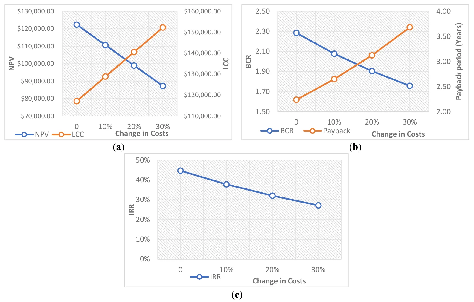
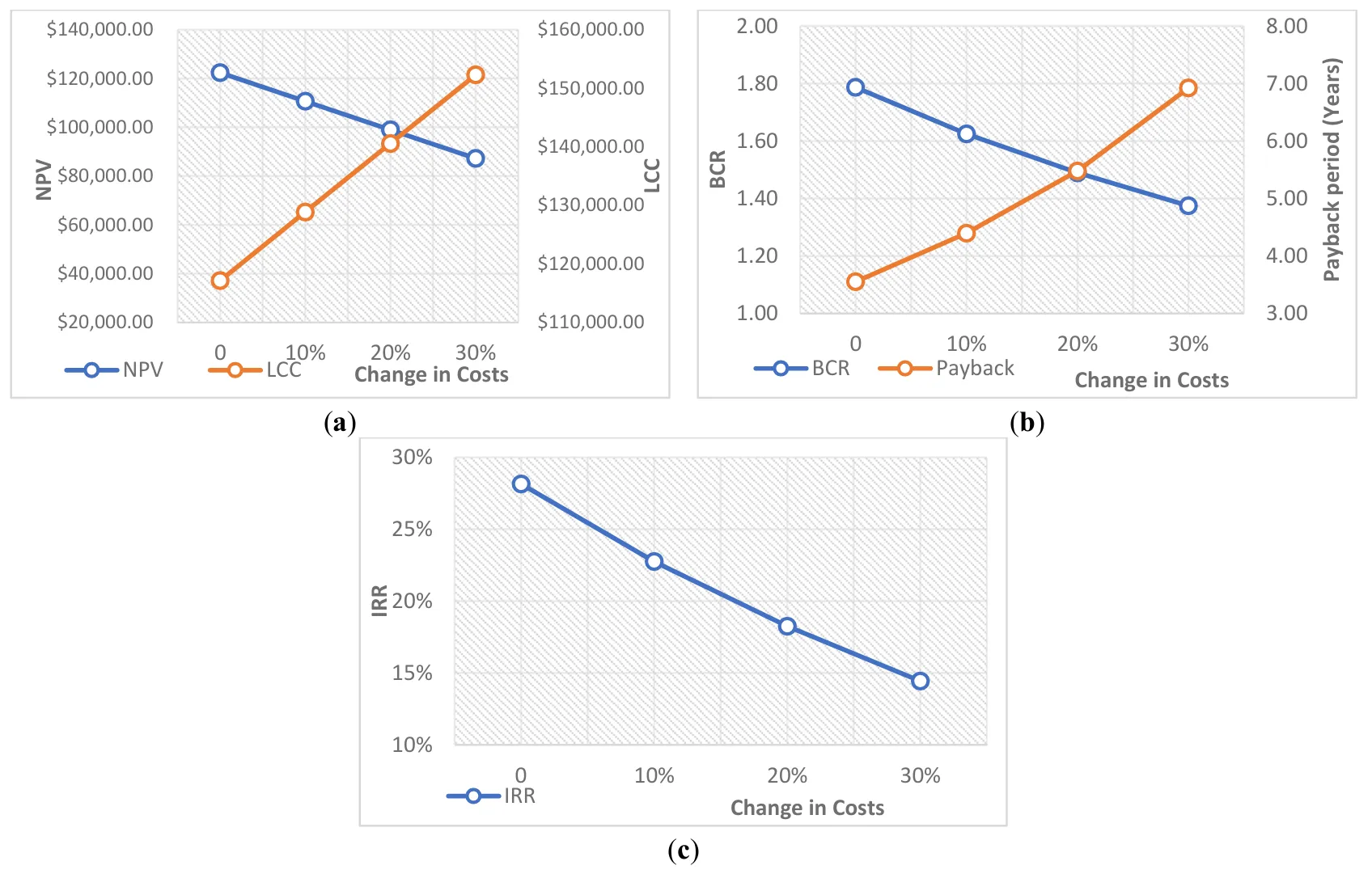
Under the 0% inflation baseline, the economic outlook is favorable. The Net Present Value (NPV) stands at $115,528.49, indicating strong long-term returns. The Internal Rate of Return (IRR) is 40%, and the Benefit-Cost Ratio (BCR) is 2.16, suggesting that the system delivers more than twice the benefit for every dollar spent. The payback period is relatively short at 2.47 years, and the total Life Cycle Cost (LCC) is $123,982.19. These values reflect a financially sound investment in a climate-impacted future.
When O&M costs increase by 10%, there is a modest reduction in economic performance. The NPV declines to $103,130.27, a reduction of roughly 11%, while IRR drops to 34%. The BCR decreases to 1.96, and the payback period extends to 2.94 years. Although these changes reflect cost sensitivity, the project remains well within viability thresholds and still offers a strong return relative to its LCC of $136,380.41.
At the 20% cost increase level, the NPV drops further to $90,732.05, and the IRR declines to 29%, indicating reduced profitability. The BCR decreases to 1.80, and the payback period extends to 3.50 years. While this reflects a tighter margin of return, the economic indicators still surpass the minimum benchmarks for viability, particularly for public sector investments that tolerate longer paybacks and lower returns in exchange for broader environmental and social benefits. The LCC at this level is $148,778.63.
Under the most severe stress condition of 30% cost inflation, the project still maintains economic viability. The NPV is $78,333.83, the IRR stands at 24%, and the BCR is 1.66. The payback period, while longer at 4.18 years, remains under a 5-year threshold, commonly used in infrastructure appraisal. The LCC rises to its maximum at $161,176.85. Despite the cumulative erosion of profitability, these values reinforce the robustness of the swale investment under plausible worst-case cost inflation scenarios.
provides a visual interpretation of these trends. Panel (a) highlights the steady increase in LCC alongside a declining NPV across inflation levels. Panel (b) shows the inverse behavior of BCR and payback period—BCR trends downward as inflation increases, while the payback period stretches accordingly. Panel (c) reveals the gradual but notable decline in IRR, from a high of 47% to 29% under the 30% scenario, indicating the diminishing marginal return of the project as cost pressures intensify.
. Economic indicators (<b>a</b>) NPV and LCC under 0–30% increases in maintenance costs. (<b>b</b>) BCR and Payback under 0–30% increases in maintenance costs. (<b>c</b>) IRR under 0–30% increases in maintenance costs.
The implications of this analysis are twofold. First, it underscores the robustness of the swale investment even under pessimistic cost escalations. Second, it emphasizes the value of minimizing long-term O&M burdens through strategic design choices. These may include the use of native or low-maintenance vegetation, modular construction to allow phased rehabilitation, and upstream sediment control to reduce debris buildup.
3.3.2. Simultaneous Inflation, Cost Increase, and Benefit Reduction
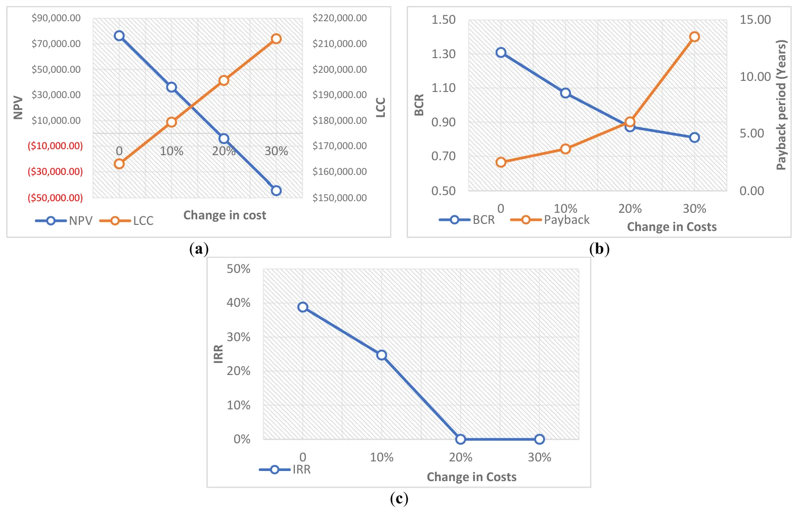
This scenario represents a compounded economic stress test designed to simulate real-world vulnerabilities affecting green infrastructure projects over time. It captures the combined effects of (a) inflationary pressures on input costs, (b) rising maintenance expenditures, and (c) declining treatment performance due to climate variability, urban densification, or swale degradation. Financial performance was evaluated under simultaneous 0%, 10%, 20%, and 30% escalations across these dimensions.
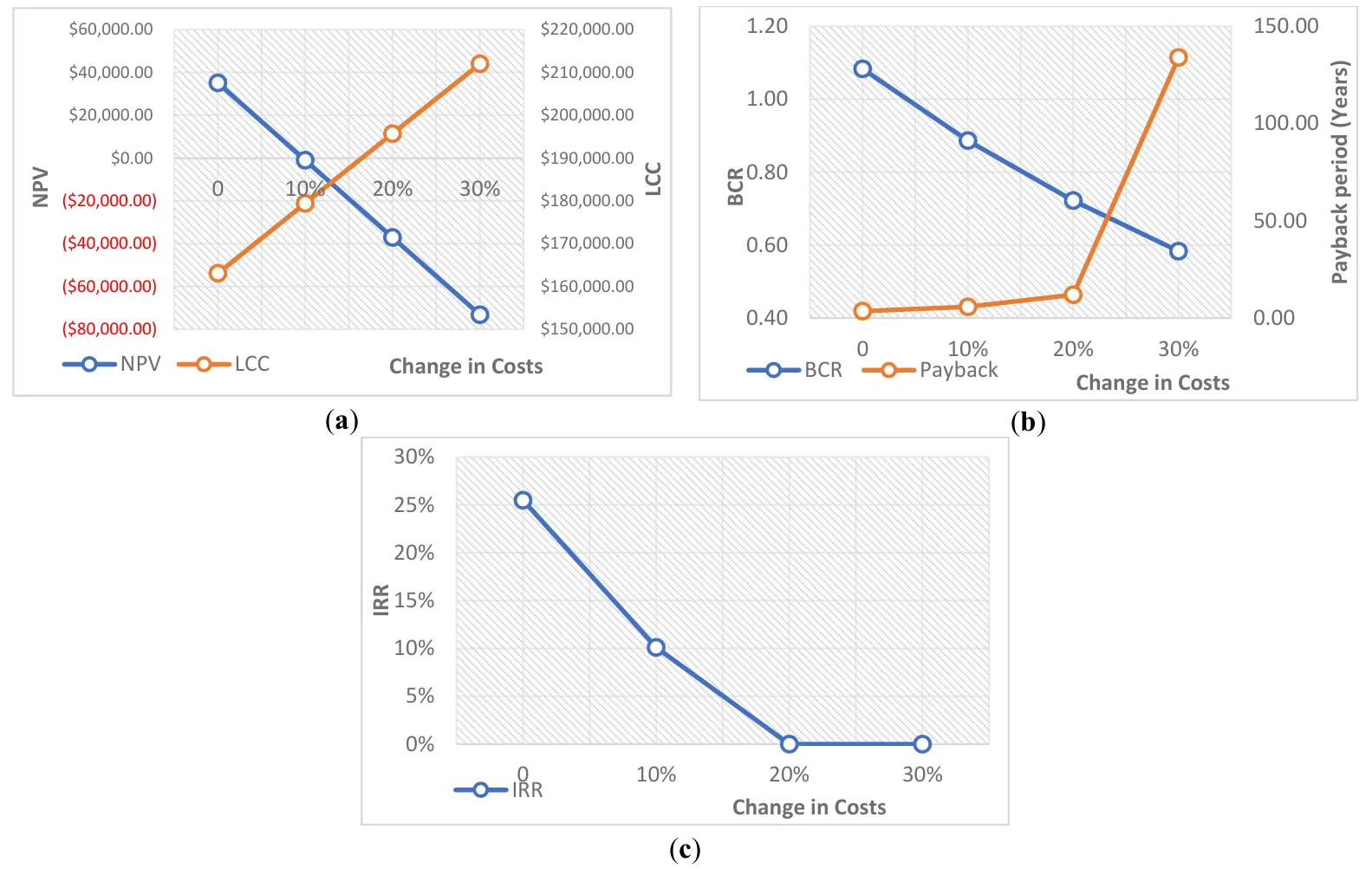
At baseline (0% stress), the swale system demonstrates robust economic viability. The Net Present Value (NPV) is $76,418.61, supported by an Internal Rate of Return (IRR) of 39%, a Benefit–Cost Ratio (BCR) of 1.31, and a short payback period of 2.47 years. With a Life-Cycle Cost (LCC) of $163,092.08, the system generates substantial economic returns, validating the investment under normal conditions.
When stress increases by 10%, performance begins to erode. The NPV falls by more than half to $36,158.33, while the IRR drops to 25%. The BCR narrows to 1.07, showing only a slim margin of benefit over cost, and the payback period is lengthened to 3.64 years. The LCC also rises to $179,401.29. At this level, the swale remains marginally viable but more vulnerable to additional pressures and reliant on sustained benefit delivery.
At 20% escalation, economic performance deteriorates further. The NPV turns slightly negative at –$4101.95, indicating a loss relative to the baseline, while the BCR drops below unity to 0.87. The payback period extends to 6.03 years, and the LCC increases to $195,710.49. The IRR becomes non-quantifiable, reflecting that the system no longer achieves breakeven under standard discounting. This suggests high sensitivity to risk and signals the need for redesign, scaling adjustments, or financial safeguards.
Under the 30% scenario, the system becomes clearly unviable. The NPV declines sharply to –$44,362.22, with the BCR at just 0.81, showing that only $0.81 of benefit is generated per dollar spent. The payback period lengthens dramatically to 13.52 years, and the LCC reaches $212,019.70. The IRR remains undefined, confirming the project’s inability to recover its investment. This outcome reflects a tipping point where the financial justification for implementation collapses, even if non-monetary co-benefits are considered.
illustrates these dynamics: panel (a) shows NPV falling into negative territory as LCC steadily rises; panel (b) captures the deterioration of BCR and the compounding extension of payback; and panel (c) highlights the collapse of IRR from 39% at baseline to a non-quantifiable state at higher stress levels, underscoring the threshold at which investment viability breaks down.
. Economic indicators (<b>a</b>) NPV and LCC under 0–30% simultaneous inflation, cost increases, and flow‐benefit reductions. Labels in parenthesis indicated in red font denotes negative NPV values. (<b>b</b>) BCR and Payback under 0–30% simultaneous inflation, cost increases, and flow‐benefit reductions. (<b>c</b>) IRR under 0–30% simultaneous inflation, cost increases, and flow‐benefit reductions.
The analysis reveals that while the swale network is resilient to moderate shocks, its economic integrity weakens significantly under higher compounded stresses. At the 20% escalation level, the system’s NPV turns slightly negative and its BCR falls below unity, signaling that the investment ceases to generate net financial returns. This transition point highlights a threshold of vulnerability where the swale remains physically functional but economically fragile, underscoring the risk of pursuing implementation without safeguards such as design optimization, scaled deployment, or performance guarantees.
The sharp deterioration observed at the 30% scenario further demonstrates the system’s susceptibility to compounded risks. At this level, the project becomes unequivocally unviable, with prolonged payback, rising life-cycle costs, and a complete breakdown of internal return measures. These results emphasize that beyond a certain escalation threshold, economic justification for nature-based solutions like swales collapses, regardless of their non-monetary co-benefits.
Accordingly, these findings reinforce the need for municipalities and implementing agencies to adopt institutional safeguards that extend beyond conventional cost–benefit analysis. Escalation clauses should be integrated into lifecycle cost assessments, and performance assumptions must be regularly recalibrated to reflect evolving climate and urban pressures. Risk-mitigation strategies—including phased upgrades, adaptive maintenance scheduling, and integration with supplemental treatment technologies—are essential to preserve economic viability under uncertainty. By embedding such mechanisms, planners can ensure that swale networks remain not only environmentally beneficial but also financially sustainable in the long term.
3.4. Economic Performance under Climate Change Scenario (RCP 8.5)
Climate change introduces long-term uncertainties that can significantly impact the performance and cost-effectiveness of nature-based infrastructure. In this analysis, a climate scenario based on RCP 8.5 was applied, incorporating a projected 15% decrease in annual rainfall volume by 2075. This reduction was used to estimate the potential drop in stormwater treatment benefits. The following subsections present economic outcomes under varied cost escalation conditions while factoring in diminished benefits due to climate change.
3.4.1. Combined Cost Inflation and Benefit Reduction
Under the RCP 8.5 climate change scenario, where a 15% reduction in rainfall is projected by 2075 despite intensifying storm events, the hydrological benefits of swale systems are expected to diminish. This section assesses how such reductions, when compounded with incremental cost increases, affect the economic viability of the swale network.
At baseline (0% increase), the system demonstrates strong financial performance. The Net Present Value (NPV) is $74,267.13, the Benefit–Cost Ratio (BCR) is 1.79, and the payback period is 3.55 years. With a Life-Cycle Cost (LCC) of $123,982.19 and an Internal Rate of Return (IRR) of 28%, the system offers a solid economic case for investment under reduced runoff benefits.
At 10% cost escalation, the system’s returns weaken but remain viable. NPV falls to $61,868.91, BCR declines to 1.62, and the payback period extends to 4.40 years. The IRR drops to 23%, while the LCC rises to $136,380.41. Although profitability is reduced, the project continues to deliver net benefits.
At 20% escalation, economic performance deteriorates further. The NPV decreases to $49,470.69, the BCR falls to 1.49, and payback extends to 5.48 years. The IRR contracts to 18%, and the LCC climbs to $148,778.63. These outcomes suggest that the system remains financially feasible but increasingly sensitive to sustained cost pressures and benefit reductions.
In the 30% scenario, the economic case weakens considerably, though it does not collapse. The NPV drops to $37,072.47, the BCR falls to 1.37, and the payback period is lengthened to 6.92 years. The IRR declines further to 14%, while the LCC peaks at $161,176.85. Despite this decline, the swale network continues to generate positive returns, albeit with much tighter margins, highlighting the importance of risk management and adaptive planning.
illustrates these results: panel (a) shows the divergence between declining NPV and rising LCC, panel (b) demonstrates the falling BCR and lengthening payback periods, and panel (c) captures the steady downward trajectory of IRR. Overall, the analysis confirms that although swale systems face economic stress under combined climate and cost pressures, they retain financial justification, supporting their role as a resilient and adaptive stormwater management measure under future conditions.
. Economic indicators under RCP 8.5 climate change scenario (<b>a</b>) NPV and LCC under 0–30% increases in maintenance costs. (<b>b</b>) BCR and Payback under 0–30% increases in maintenance costs. (<b>c</b>) IRR under 0–30% increases in maintenance costs.
3.4.2. Economic Performance Under Cost Increase, Benefit Reduction, and Inflation
Under the RCP 8.5 climate change scenario, where reduced flow-derived benefits are expected due to declining rainfall volumes despite intensifying extremes, the economic robustness of the swale network was assessed under compounded stresses of rising costs, benefit reductions, and inflationary pressures. Performance was tested at 0%, 10%, 20%, and 30% escalation levels to simulate worst-case conditions in a changing climate and economic landscape.
At the baseline (0% stress), the swale system demonstrates modest but positive viability. The Net Present Value (NPV) is $35,157.24, supported by an Internal Rate of Return (IRR) of 25% and a Benefit–Cost Ratio (BCR) of 1.08. The payback period is 3.55 years, with a Life-Cycle Cost (LCC) of $163,092.08. These figures suggest that the system remains investable under current conditions, though its margin of resilience is relatively narrow.
At the 10% escalation level, the project’s financial position weakens considerably. The NPV turns slightly negative at –$976.90, the IRR declines to 10%, and the BCR drops below unity to 0.89, indicating that costs begin to outweigh discounted benefits. The payback period is lengthened to 5.76 years, while the LCC rises to $179,401.29. This marks the tipping point, where economic performance shifts from viable to marginal.
Under 20% stress, the system becomes economically infeasible. The NPV falls to –$37,111.04, the BCR declines further to 0.72, and the payback period extends to 11.97 years. The IRR becomes undefined, reflecting that the project cannot achieve breakeven under standard discount rates. With the LCC increasing to $195,710.49, the system incurs a clear financial deficit, undermining its justification as an investment option.
At the most severe case of 30% escalation, the swale system becomes wholly unsustainable. The NPV plunges to –$73,245.18, the BCR contracts to just 0.58, and the payback period balloons to an impractical 133.92 years. The IRR remains undefined, while the LCC peaks at $212,019.70. This outcome illustrates the collapse of financial viability under high-stress climate and economic conditions associated with RCP 8.5.
illustrates these trajectories: panel (a) highlights the steady increase in LCC against declining NPV, panel (b) shows the worsening BCR and accelerating payback periods, and panel (c) captures the collapse of IRR beyond the 10% threshold. Collectively, the results highlight the fragility of the swale system’s economic performance under RCP 8.5 and reinforce the need for adaptive design strategies, escalation-adjusted budgeting, and proactive asset management to preserve long-term viability.
. Economic indicators under RCP 8.5 climate change scenario (<b>a</b>) NPV and LCC under 0–30% simultaneous inflation, cost increases, and flow‐benefit reductions. Labels in parenthesis indicated in red font denotes negative NPV values. (<b>b</b>) BCR and Payback under 0–30% simultaneous inflation, cost increases, and flow‐benefit reductions. (<b>c</b>) IRR under 0–30% simultaneous inflation, cost increases, and flow‐benefit reductions.
4. Conclusions
This study demonstrated that vegetated swales are both a technically sound and economically viable nature-based solution (NbS) for urban stormwater management, particularly within the South Australian context and with broader implications for similar urban catchments. The application of the MUSICX hydrological model and a detailed case study based in the City of Onkaparinga, the research successfully quantified the pollution removal potential and economic performance of a networked swale system.
From a technical standpoint, the swale network achieved consistently high removal efficiencies for key stormwater pollutants, including Total Suspended Solids (TSS), Total Nitrogen (TN), and Total Phosphorus (TP), as well as gross pollutants. These results indicate the system’s effectiveness in delivering essential water quality improvements, reinforcing the role of swales as a core Water Sensitive Urban Design (WSUD) intervention.
Economically, the swale system yielded strong lifecycle performance. Under baseline assumptions, key indicators such as Net Present Value (NPV), Internal Rate of Return (IRR), and Benefit-Cost Ratio (BCR) significantly exceeded standard viability thresholds. Importantly, the system’s payback period remained relatively short—typically under three years—demonstrating the project’s capacity for timely returns relative to investment. The results remained positive even under moderately adverse scenarios involving inflationary pressures and increased operation and maintenance (O&M) costs.
Sensitivity analyses, including stress-testing for up to 30% increases in lifecycle costs and reductions in pollutant-treatment benefits, revealed important insights into the system’s economic resilience. While profitability naturally declined under such stressful conditions, the swale network retained financial viability up to a certain threshold. For example, the BCR remained above 1.0 and NPV stayed positive in all but the most extreme combined stress scenarios.
Climate change scenarios (based on RCP 8.5 projections), which accounted for a 15% decline in effective rainfall and inflow volumes by 2075, further tested the robustness of the system. Even when paired with rising O&M costs and diminishing pollutant loads, the swale network demonstrated economic feasibility under all but the most severe stress conditions, underscoring its long-term sustainability if appropriately managed.
The findings also revealed a key insight: while payback period remains a useful metric, it may be misleading under extreme economic pressure. In such conditions, payback may appear to improve (i.e., become shorter), even as NPV turns negative and BCR falls below 1.0, indicating an economically unviable project. This reinforces the need to interpret payback in tandem with other economic indicators to gain a full picture of project viability.
The study concludes that vegetated swales, when properly designed and maintained, offer a reliable and cost-effective solution for urban runoff treatment. Their performance holds up under varying economic and climatic scenarios, making them suitable for adoption within urban stormwater management frameworks not only in Australia but also in developing countries such as the Philippines. The research supports the integration of swales into WSUD guidelines and underscores the importance of ongoing maintenance, adaptive management, and climate-aware planning to ensure long-term effectiveness and economic sustainability.
Acknowledgments
The authors gratefully acknowledge Chris Chow, Course Coordinator for the Master’s Research Project at the University of South Australia, for his academic leadership and guidance during the early stages of the study. His insights helped refine the research direction and align it with broader program objectives. The authors also thank the academic and technical staff of UniSA STEM for their support throughout the project. Contributions in the form of coursework, modelling advice, and consultations were instrumental in applying theoretical concepts to real-world challenges. The authors further acknowledge the University of South Australia for providing access to licensed software essential to the modelling and analysis tasks of this study. Appreciation is also extended to the City of Onkaparinga for their cooperation and provision of site-specific information, planning data, and background documentation. This support was essential in ensuring that the case study design reflected practical and contextual realities.
Author Contributions
Conceptualization, F.B.d.G. and F.A.A.; Methodology, F.B.d.G.; Software, F.B.d.G.; Validation, F.B.d.G., N.P., R.J.P. and J.K.Y.; Formal Analysis, J.K.Y.; Investigation, N.P. and R.J.P.; Resources, F.B.d.G., N.P., R.J.P. and J.K.Y.; Data Curation, F.B.d.G.; Writing – Original Draft Preparation, F.B.M.d.G, N.P., R.J.P. and J.K.Y.; Writing – Review & Editing, F.B.d.G. and F.A.A.; Visualization, J.K.Y.; Supervision, F.A.A.; Project Administration, F.B.d.G. and F.A.A.
Ethics Statement
Not applicable.
Informed Consent Statement
Not applicable.
Data Availability Statement
Data of this research article may be available upon request to authors.
Funding
This study was completed as a part of Master of Engineering thesis at the University of South Australia and no extra funding was involved.
Declaration of Competing Interest
The authors declare that they have no known competing financial interests or personal relationships that could have appeared to influence the work reported in this paper.
References
-
1.
Winston RJ, Anderson AR, Hunt WF. Modeling Sediment Reduction in Grass Swales and Vegetated Filter Strips Using Particle Settling Theory. J. Environ. Eng. 2017, 143. doi:10.1061/(ASCE)EE.1943-7870.0001162.
-
2.
Jia H, Jia H, Hu J, Huang T, Chen AS, Ma Y. Urban Runoff Control and Sponge City Construction; MDPI Books: Basel, Switzerland, 2022.
-
3.
Roy AH, Wenger SJ, Fletcher TD, Walsh CJ, Ladson AR, Shuster WD, et al. Impediments and solutions to sustainable, watershed-scale urban stormwater management: lessons from Australia and the United States.
Environ. Manag. 2008,
42, 344–359.
[Google Scholar]
-
4.
Wong THF. An Overview of Water Sensitive Urban Design Practices in Australia.
Water Pract. Technol. 2006,
1, doi:10.2166/wpt.2006018.
[Google Scholar]
-
5.
Ahammed F. A review of water-sensitive urban design technologies and practices for sustainable stormwater management.
Sustain. Water Resour. Manag. 2017, doi:10.1007/s40899-017-0093-8.
[Google Scholar]
-
6.
Hunt WF, Davis AP, Traver RG. Meeting Hydrologic and Water Quality Goals through Targeted Bioretention Design.
J. Environ. Eng. 2012,
138, 698–707, doi:10.1061/(ASCE)EE.1943-7870.0000504.
[Google Scholar]
-
7.
Kim H, Seagren EA, Davis AP. Engineered Bioretention for Removal of Nitrate from Stormwater Runoff.
Water Environ. Res. 2003,
75, 355–367, doi:10.2175/106143003X141169.
[Google Scholar]
-
8.
Ristianti NS, Bashit N, Ulfiana D, Windarto YE. Bioretention Basin, Rain Garden, and Swales Track Concepts through Vegetated-WSUD: Sustainable Rural Stormwater Management in Klaten Regency. In Proceedings of 2nd International Conference on Urban Design and Planning "Sustainable Urban Design and Development in Post-Pandemic World", online, 2022; p. 012029.
-
9.
Liu G, Xie C, Zhao L, Xiao Y, Wu T, Wang W, et al. Permafrost warming near the northern limit of permafrost on the Qinghai–Tibetan Plateau during the period from 2005 to 2017: A case study in the Xidatan area.
Permafrost and Periglac. Proc. 2021,
32, 323–334, doi:10.1002/ppp.2089.
[Google Scholar]
-
10.
Venter ZS, Barton DN, Martinez-Izquierdo L, Langemeyer J, Baró F, McPhearson T. Interactive spatial planning of urban green infrastructure – Retrofitting green roofs where ecosystem services are most needed in Oslo.
Ecosyst. Serv. 2021,
50, 101314, doi:10.1016/j.ecoser.2021.101314.
[Google Scholar]
-
11.
Abida H, Sabourin JF. Grass Swale-Perforated Pipe Systems for Stormwater Management.
J. Irrigation Drainage Eng. 2006,
132, 55–63, doi:10.1061/(asce)0733-9437(2006)132:1(55).
[Google Scholar]
-
12.
Department of Planning and Local Government. Water Sensitive Urban Design Technical Manual for the Greater Adelaide Region. 2010. Available online: https://www.watersensitivesa.com/resources/guidelines/design/design-wsud-all-assets/technical-manual-for-water-sensitive-urban-design-in-greater-adelaide/ (accessed on 3 March 2025).
-
13.
Saraçoğlu KE, Kazezyılmaz-Alhan CM. Determination of grass swale hydrological performance with rainfall-watershed-swale experimental setup.
J. Hydrol. Eng. 2023,
28, 04022043.
[Google Scholar]
-
14.
Wang X, Zhang R, Hu Q, Sun C, Ikram RMA, Wang M, et al. Assessment of the Hydrological Performance of Grass Swales for Urban Stormwater Management: A Bibliometric Review from 2000 to 2023.
Water 2025,
17, 1425.
[Google Scholar]
-
15.
Mantilla I, Muthanna TM, Marsalek J, Viklander M. Assessing spatial and temporal variability of grass swale infiltration in shallow groundwater conditions.
J. Environ. Eng. 2025,
380, 124977.
[Google Scholar]
-
16.
Mantilla I, Flanagan K, Broekhuizen I, Muthanna TM, Marsalek J, Viklander M. Retrofit of grass swales with outflow controls for enhancing drainage capacity.
J. Hydrol. 2024,
639, 131637.
[Google Scholar]
-
17.
Gavrić S, Leonhardt G, Österlund H, Marsalek J, Viklander M. Metal enrichment of soils in three urban drainage grass swales used for seasonal snow storage.
Sci. Total Environ. 2021,
760, 144136.
[Google Scholar]
-
18.
Gavric S. Enhancement of stormwater quality in grass swales: Removal and immobilisation of metals. Licentiate Thesis, Department of Civil, Environmental and Natural Resources Engineering, Luleå University of Technology, Luleå, Sweden, 2020.
-
19.
Zaqout T, Andradóttir H. Infiltration Capacity in Grass Swales During Frequent Freeze‐Thaw Cycles and Intermittent Snowmelt in a Cold Maritime Climate. In Proceedings of the 15th International Conference on Urban Drainage, Melbourne, Australia, 25–28 Oct 2021.
-
20.
Ekka SA, Hunt III WF, McLaughlin RA. Systematic evaluation of swale length, shape, and longitudinal slope with simulated highway runoff for better swale design.
Environ. Sci. Pollut. Res. 2024, doi:10.1007/s11356-024-35474-1.
[Google Scholar]
-
21.
Salim MIIA, Aliza N. A performance review of grass swales channel in Malaysia.
Recent Trends Civil Eng. Built Environ. 2022,
3, 663–671.
[Google Scholar]
-
22.
Ruibin Z. Comparison of the effect of two kinds of ecological grass swales on road runoff purification.
J. Environ. Eng. Technol. 2021,
11, 493–498.
[Google Scholar]
-
23.
Wang J, Qiu R, Xia X, Li X, Zhang C, Wang W. A Modified Manning’s Equation for Estimating Flow Rate in Grass Swales under Low Inflow Rate Conditions.
Water 2024,
16, 1613.
[Google Scholar]
-
24.
Saraçoğlu KE, Kazezyılmaz‐Alhan CM. Development of a hydrological model for vegetated swales under different rainfall and swale properties.
Water Environ. Res. 2025,
97, e70014.
[Google Scholar]
-
25.
Yang F, Fu D, Zevenbergen C, Boogaard FC, Singh RP. Time-varying characteristics of saturated hydraulic conductivity in grassed swales based on the ensemble Kalman filter algorithm—A case study of two long-running swales in Netherlands.
J. Environ. Manag. 2024,
351, 119760.
[Google Scholar]
-
26.
Yang F, Fu D, Zevenbergen C, Boogaard FC, Singh RP. Screening of representative rainfall event series for long-term hydrological performance evaluation of grassed swales.
Environ. Sci. Pollut. Res. 2024, doi:10.1007/s11356-024-32355-5.
[Google Scholar]
-
27.
Mantilla I, Flanagan K, Broekhuizen I, Muthanna T, Viklander M. Evaluating the infiltration performance of grassed swales: Comparison between point measurements and a full-scale infiltration method. In Proceedings of the Novatech 2023, Lyon, France, 2023.
-
28.
Lu L, Chan FKS, Johnson M, Zhu F, Xu Y. The development of roadside green swales in the Chinese Sponge City Program: Challenges and opportunities.
Front. Eng. Manag. 2023,
10, 566–581.
[Google Scholar]
-
29.
Mehta O, Kansal ML, Bisht DS. A comparative study of the time of concentration methods for designing urban drainage infrastructure.
Water Infrastruct., Ecosyst. Soc. 2022,
71, 1197–1218, doi:10.2166/aqua.2022.107.
[Google Scholar]
-
30.
Vasiliades L, Farsirotou E, Psilovikos A. An Integrated Hydrologic/Hydraulic Analysis of the Medicane "Ianos" Flood Event in Kalentzis River Basin, Greece. In Proceedings of the 7th IAHR Europe Congress, Athens, Greece, 2022.
-
31.
Leivadiotis E, Psilovikos A. A Performance Evaluation and Statistical Analysis of IMERG Precipitation Products During Medicane Daniel (September 2023) in the Thessaly Plain, Greece.
Water 2025,
17, 2401.
[Google Scholar]
-
32.
Soria JM, Muñoz R, Campillo-Tamarit N, Molner JV. Flash-Flood-Induced Changes in the Hydrochemistry of the Albufera of Valencia Coastal Lagoon.
Diversity 2025,
17, 119, doi:https://doi.org/10.3390/d17020119.
[Google Scholar]
-
33.
Sciuto L, Licciardello F, Giuffrida ER, Barresi S, Scavera V, Verde D, et al. Hydrological-hydraulic modelling to assess Nature-Based Solutions for flood risk mitigation in an urban area of Catania (Sicily, Italy).
Nat.-Based Solut. 2025,
7, 100210, doi:https://doi.org/10.1016/j.nbsj.2024.100210.
[Google Scholar]
-
34.
Ball J, Babister M, Nathan R, Weeks B, Weinmann E, Retallick M, et al. (Eds.) Australian Rainfall and Runoff: Book 5–Flood Hydrograph Estimation, Revision 4.2 ed.; Commonwealth of Australia (Geoscience Australia): Canberra, Australia, 2019; p. 30.
-
35.
Argue JR. Storm drainage design in small urban catchments: a handbook for Australian practice; Australian Road Research Board: Melbourne, Australia, 1986.
-
36.
Meteorology Bo. Design Rainfall Data System. 2016. Available online: http://www.bom.gov.au/water/designRainfalls/revised-ifd/?coordinate_type=dd&latitude=-35.265&longitude=138.482&user_label=&design=ifds&sdmin=true&sdhr=true&sdday=true (accessed on 10 March 2025).
-
37.
Trade waste fees and charges. Available online: https://www.sawater.com.au/my-business/trade-waste/trade-waste-management/trade-waste-fees-and-charges (accessed on 10 March 2025).
-
38.
Water and Sewerage prices. Available online: https://www.sawater.com.au/__data/assets/pdf_file/0011/941348/2024-25-Price-setting-Water-and-Sewerage-prices.pdf (accessed on 10 March 2025).