A Quadrotor Simulation and Research Platform

Munasinghe, Sudath  Rohan

doi:10.70322/dav.2025.10014

Article Open Access

A Quadrotor Simulation and Research Platform

Sudath Rohan Munasinghe ^1,2,*

Author Information

Other Information

College of Agriculture and Life Sciences, Cornell University, Ithaca, NY 18450, USA

Department of IT and Entrepreneurship, Narva College, Tartu University, 50090 Tartu, Estonia

Authors to whom correspondence should be addressed.

Received: 10 April 2025 Revised: 18 June 2025 Accepted: 01 August 2025 Published: 17 September 2025

Views:712

Downloads:210

Drones Veh. Auton. 2025, 2(3), 10014; DOI: 10.70322/dav.2025.10014

ABSTRACT: The quadrotor is an underactuated, nonlinear system that presents significant challenges in both modeling and control design. This work develops a decoupled control framework based on the translational (Newtonian) and rotational (Eulerian) dynamics of the quadrotor. A Linear Quadratic Gaussian (LQG) regulator is implemented for control, with two extended Kalman filters employed for state estimation in the respective dynamic subsystems. The full design process, from dynamic modeling to flight simulation presented in detail. Key elements include nonlinear simulation, model linearization, state-space representation, feedforward compensation, Linear Quadratic Regulator (LQR) gain tuning, actuator dynamics, sensor noise, LQG design, and extended Kalman filter. The limitations of applying linear control to a nonlinear system are also presented.

Keywords: Quadrotor dynamic modeling; Mechanics and control of quadrotor; Sensor-based quadrotor control; Linear quadratic regulator; Extended kalman filter

1. Introduction

The quadrotor is a complex system characterized by nonlinear dynamics, controllability challenges due to linearization, actuator saturation, and the need for accurate state estimation [1]. Quadrotors have already become an integral part of modern society and are widely deployed across various application domains [2]. Numerous control strategies have been developed and published, including PID [3], Fuzzy-PID [4], Linear Quadratic Regulator (LQR) [5], and various forms of the backstepping algorithm [6]. More recently, research has expanded into advanced control topics such as fault-tolerant systems and reinforcement learning [7], deep reinforcement learning for parameter identification [8], sliding mode control [9], adaptive neuro-fuzzy control [10], deep learning-based control [11], and robust model reference adaptive control [12]. Despite this progress, a noticeable gap remains in the literature regarding the integration and testing of different subsystems within a complete quadrotor system. The sequential development of the system, from initial modeling through to simulation and validation is rarely documented in a unified manner. This work aims to address that gap by presenting a comprehensive treatment of the quadrotor system, including all critical stages from dynamic modeling to flight simulation. The translational and rotational dynamics of the quadrotor are modeled separately and coupled through a rotation matrix. Gravity is treated as a persistent disturbance, and a hover thrust is introduced as a feedforward control input to compensate for it. This approach simplifies the state-space modeling and facilitates the implementation of a Linear Quadratic Regulator (LQR). The actuator dynamics are represented using the transfer function of a brushless motor. For state estimation, two extended Kalman filters (EKFs) are employed: one for estimating the translational states and another for estimating the body rates, from which the rotational states are inferred. The LQR controller is designed based on the full set of estimated states. This paper also addresses several critical aspects of control system design for quadrotors: (1) linearizing the nonlinear dynamics without compromising controllability, (2) identifying disturbance inputs and applying feedforward control to compensate for them, (3) determining an appropriate control loop frequency based on actuator rise time, and (4) designing multiple extended Kalman filters for a complex, multi-subsystem model. The paper is organized as follows: Section 2 presents the quadrotor dynamic model as two separate submodels for translational and rotational motions. Section 3 presents the model linearization and linear state space model of the quadrotor. Section 4 presents the linear quadratic regulator. Section 5 presents how actuator dynamics and sensors are included in the system. Section 6 presents the LQG, which includes sensor integration and EKF state estimation to get rid of sensor noise. Section 7 presents the results, and Section 8 provides the conclusions.

2. Dynamic Modeling of a Quadrotor

2.1. Translational Motion Figure 1 shows a quadrotor [B] after undergoing a translational motion (x, y, z) and a rotational motion (ψ, θ, $$\phi$$) with respect to the Earth frame [E]. The lift forces generated by the four propellers are f₁, f₂, f₃, f₄; hence, the net upward force with respect to [B] is given by:

Figure 1. Quadrotor forces torques and motion.

```latex\begin{array}{ccc}F&=&f_1+f_2+f_3+f_4\end{array}```

(1)

```latex \quad\quad\quad\quad\quad =\quad k_f(\omega_1^2+\omega_2^2+\omega_3^2+\omega_4^2)```

(2)

where k_f is the lift coefficient and ω_i; i = 1, 2, 3, 4 are propeller speeds (RPM). The linear motion of the quadrotor with respect to [E] is described using Newton’s laws of motion as follows:

```latex \begin{bmatrix}\ddot{x}\\\ddot{y}\\\ddot{z}\end{bmatrix}=\frac{1}{m}_B^ER(\psi,\theta,\phi)\begin{bmatrix}0\\0\\F\end{bmatrix}+\begin{bmatrix}0\\0\\-g\end{bmatrix}-\frac{1}{m}C_d\begin{bmatrix}\dot{x}\\\dot{y}\\\dot{z}\end{bmatrix} ```

(3)

In this equation, the first term on the right-hand side represents the acceleration of the quadrotor due to the propeller force acting along ^Bz, transformed to the Earth frame [E] using the z-y-x Euler rotation matrix (A4). The second term corresponds to the acceleration caused by gravity, which acts vertically downward with respect to [E]. The third term accounts for the deceleration of the quadrotor due to air drag. The air drag matrix C_d, which includes the drag coefficients C_x, C_y, C_z along the x -, y -, and z -directions, is given by:

```latexC_d=\begin{bmatrix}C_x&0&0\\0&C_y&0\\0&0&C_z\end{bmatrix}```

By expanding Equation (3), the three translational acceleration components of the quadrotor are obtained as follows:

```latex \begin{array}{ccc}\ddot{x}&=&(\cos\psi\sin\theta\cos\phi+\sin\psi\sin\phi)\frac{F}{m}-\frac{C_x}{m}\dot{x}\end{array}```

(4)

```latex \begin{array}{ccc}\ddot{y}&=&(\sin\psi\sin\theta\cos\phi+\cos\psi\sin\phi)\frac{F}{m}-\frac{C_y}{m}\dot{y}\end{array}```

(5)

```latex \begin{array}{rcl}\ddot{z}&=&\cos\theta\cos\phi\frac{F}{m}-\frac{C_z}{m}\dot{z}-g\end{array}```

(6)

2.2. Rotational Motion As shown in Figure 1, the propeller forces acting at a distance l from the center of mass generate torques τ_x, τ_y, and τ_z about the principal axes of the quadrotor.

```latex \begin{array}{ccc}\tau_x&=&k_fl(\omega_4^2-\omega_2^2)\end{array}```

(7)

```latex \begin{array}{ccc}\tau_y&=&k_fl(\omega_1^2-\omega_3^2)\end{array}```

(8)

```latex \begin{array}{rcl}\tau_z&=&k_m(\omega_1^2-\omega_2^2+\omega_3^2-\omega_4^2)\end{array}```

(9)

The torques τ_x and τ_y are produced by the thrust forces generated by the propellers, while τ_z results from the aerodynamic drag of the propellers. The symbol k_m denotes the propeller drag coefficient. These torques induce rotational motion in the quadrotor. According to Euler’s rotational dynamics, τ = Iω + ω × Iω, the rotational motion of the quadrotor can be expressed as follows:

```latex \begin{aligned}\begin{bmatrix}\tau_x\\\tau_y\\\tau_z\end{bmatrix}&=\begin{bmatrix}I_x&0&0\\0&I_y&0\\0&0&I_z\end{bmatrix}\begin{bmatrix}\dot{\omega}_x\\\dot{\omega}_y\\\dot{\omega}_z\end{bmatrix}+\begin{bmatrix}\omega_x\\\omega_y\\\omega_z\end{bmatrix}\times\begin{bmatrix}I_x&0&0\\0&I_y&0\\0&0&I_z\end{bmatrix}\begin{bmatrix}\omega_x\\\omega_y\\\omega_z\end{bmatrix}\\&=\quad\begin{bmatrix}I_x\dot{\omega}_x\\I_y\dot{\omega}_y\\I_z\dot{\omega}_z\end{bmatrix}+\begin{bmatrix}\omega_x\\\omega_y\\\omega_z\end{bmatrix}\times\begin{bmatrix}I_x\omega_x\\I_y\omega_y\\I_z\omega_z\end{bmatrix}\\&=\quad\begin{bmatrix}I_x\dot{\omega}_x\\I_y\dot{\omega}_y\\I_z\dot{\omega}_z\end{bmatrix}+\begin{bmatrix}(I_z-I_y)\omega_y\omega_z\\(I_x-I_z)\omega_x\omega_z\\(I_y-I_x)\omega_x\omega_y\end{bmatrix}\end{aligned} ```

(10)

where I_x, I_y, and I_z are the moments of inertia of the quadrotor about the axes ^Bx, ^By, and ^Bz, respectively. It is assumed that the three principal axes of the quadrotor are aligned with ^Bx, ^By, and ^Bz, such that the products of inertia between these axes are zero. From Equation (10), the angular accelerations of the quadrotor about the axes ^Bx, ^By, and ^Bz are derived as follows:

```latex \dot{\omega}_x\quad=\quad[\tau_x-(I_z-I_y)\omega_y\omega_z]/I_x ```

(11)

```latex \begin{array}{ccc}\dot{\omega}_y&=&[\tau_y-(I_x-I_z)\omega_x\omega_z]/I_y\end{array} ```

(12)

```latex \dot{\omega}_z\quad=\quad[\tau_z-(I_y-I_x)\omega_x\omega_y]/I_z ```

(13)

These equations describe how the quadrotor executes rolling, pitching, and yawing motions in response to the torques τ_x, τ_y, and τ_z. 2.3. System Parameters A custom-built quadrotor is used for the estimation of system parameters. The total weight of the quadrotor is 0.730 kg, with each motor and propeller assembly weighing 0.082 kg. The diagonal motor-to-motor distance measures 0.36 m. Accordingly, the principal moments of inertia are approximately calculated as I_x = 5.0 × 10⁻³, I_y = 6.0 × 10⁻³, and I_z = 8.0 × 10⁻³. Typical values for other parameters are k_f = 2.7 × 10⁻⁶ and k_m = 2.1 × 10⁻⁷. From Equation (2), the propeller RPM required for the quadrotor to hover is computed as follows:

```latex \omega_h=\sqrt{\frac{mg}{4k_f}}=814.3RPM ```

(14)

3. Model Linearization at Hover State

The equations of motion for the quadrotor, given by (4)–(6) and (11)–(13), capture the nonlinear dynamics that must be linearized around an appropriate flight condition to enable the design of a linear controller. For this purpose, the hover state is selected as the operating point for model linearization. 3.1. Linearization of Translational Dynamics At the hover state, the pitch and roll angles are zero, i.e., θ = $$\phi$$ = 0, while the yaw angle ψ can assume any heading. For simplicity, ψ = 0 is assumed. The vertical force balance at hover is given by F_h = mg. Under these conditions, the translational dynamics described in (4)–(6) are linearized as follows:

```latex \ddot{x}\quad=\quad g\theta-\frac{C_x}{m}\dot{x} ```

(15)

```latex \ddot{y}\quad=\quad-g\phi-\frac{C_y}{m}\dot{y} ```

(16)

```latex \begin{array}{ccc}\ddot{z}&=&\frac{1}{m}F-\frac{C_z}{m}\dot{z}-g\end{array} ```

(17)

It is important to note that the total vertical force is given by F = F_h + ∆F , where the imbalance component ∆F generates the vertical acceleration $$\ddot{z}$$. 3.2. Linearization of Rotational Dynamics At the hover state, the body angular rates are very small; therefore, assuming $$\dot{\omega}_x\dot{\omega}_y\approx\dot{\omega}_y\dot{\omega}_z\approx\dot{\omega}_x\dot{\omega}_z\approx0$$, the rotational dynamics in (11)–(13) can be linearized as follows:

```latex \begin{array}{ccc}\dot{\omega}_x&=&\tau_x/I_x\end{array} ```

(18)

```latex \begin{array}{ccc}\dot{\omega}_y&=&\tau_y/I_y\end{array} ```

(19)

```latex \begin{array}{ccc}\dot{\omega}_z&=&\tau_z/I_z\end{array} ```

(20)

From Equation (A11), the Euler anguler rates corresponding to the body angular rates at a given Euler orientation are expressed as follows:

```latex \begin{array}{rcl}\dot{\psi}&=&(\sin\phi\omega_y+\cos\phi\omega_z)/\cos\theta\end{array} ```

(21)

```latex \begin{array}{ccc}\dot{\theta}&=&\cos\phi\omega_y-\sin\phi\omega_z\end{array}```

(22)

```latex \begin{array}{rcl}\dot{\phi}&=&\omega_x+\tan\theta\sin\phi\omega_y+\tan\theta\cos\phi\omega_z\end{array}```

(23)

By differentiation, Euler angular accelerations are obtained as follows:

```latex \ddot{\psi}=\quad\frac{c\theta(s\phi\dot{\omega}_{y}+\omega_{y}\dot{\phi}c\phi)+s\phi\omega_{y}s\theta\dot{\theta}}{c^{2}\theta}+\\ \,\,\,\,\,\,\,\,\,\,\,\,\,\,\frac{c\theta(c\phi\dot{\omega}_{z}-\omega_{z}s\phi\dot{\phi})+c\phi\omega_{z}s\theta\dot{\theta}}{c^{2}\theta}```

(24)

```latex \begin{array}{ccc}\ddot{\theta}&=&c\phi\dot{\omega}_y-s\phi\omega_y\dot{\phi}-s\phi\dot{\omega}_z-\omega_zc\phi\dot{\phi}\end{array} ```

(25)

```latex \ddot{\phi}=\quad\dot{\omega}_{x}+t\theta S\phi\dot{\omega}_{y}+\omega_{y}(t\theta c\phi\dot{\phi}+s\phi\dot{\theta}/c^{2}\theta)+\\ t\theta c\phi\dot{\omega}_{z}+\omega_{z}(c\phi\dot{\theta}/c^{2}\theta-t\theta s\phi\dot{\phi}) ```

(26)

Due to the fact that θ ≈ $$\phi$$ ≈ 0 at the hover state,

```latex \begin{array}{ccc}\ddot{\psi}&=&\dot{\omega}_{z}+\omega_{y}\dot{\phi}\end{array} ```

(27)

```latex\begin{array}{ccc}\ddot{\theta}&=&\dot{\omega}_{y}-\omega_{z}\dot{\phi}\end{array} ```

(28)

```latex \begin{array}{ccc}\ddot{\phi}&=&\dot{\omega_{x}}+\omega_{z}\dot{\theta}\end{array} ```

(29)

Then, because $$\omega_{y}\dot{\phi}\approx\omega_{z}\dot{\phi}\approx\omega_{z}\dot{\theta}\approx0$$ at hover state,

```latex \begin{array}{ccc}\ddot{\psi}&=&\dot{\omega}_z\end{array} ```

(30)

```latex \begin{array}{ccc}\ddot{\theta}&=&\dot{\omega}_y\end{array} ```

(31)

```latex \begin{array}{ccc}\ddot{\phi}&=&\dot{\omega}_x\end{array} ```

(32)

Therefore, from Equation (18), Equation (19) and Equation (20), the linearized Euler angular accelerations are as follows:

```latex \begin{array}{ccc}\ddot{\psi}&=&\tau_x/I_x\end{array} ```

(33)

```latex \begin{array}{ccc}\ddot{\theta}&=&\tau_y/I_y\end{array} ```

(34)

```latex \begin{array}{rcl}\dot{\phi}&=&\tau_z/I_z\end{array} ```

(35)

3.3. State Space Model of the Quadrotor From the linearized translational dynamics (15)–(17), translational states and control input are identified as x, y, z and F. From the linearized rotational dynamics (33)–(35), the rotational states and respective control inputs are identified as ψ, θ, $$\phi$$, and τ_z, τ_y, τ_z, respectively. Then, the state vector and the control vector are assembled as ($$x,y,z,\dot{x},\dot{y},\dot{z},\psi,\theta,\phi,\dot{\psi},\dot{\theta},\dot{\phi}$$)^T, and $$(F,\tau_z,\tau_y,\tau_z)^T$$ . Linearized dynamics can be arranged into the state space model [13] shown below.

```latex \dot{\mathbf{x}}(t)_{12\times1}=\mathbf{A}_{12\times12}\mathbf{x}(t)_{12\times1}+\mathbf{B}_{12\times4}\mathbf{u}(t)_{4\times1}```

The state-space model is presented in detail in (36). However, the acceleration due to gravity term −g in (17) is not included explicitly in the state-space model (36); instead, it is treated as a persistent disturbance within the translational dynamics. The force required to counteract gravity, F_h = mg, is introduced as a feedforward input. This approach relieves the feedback control system from having to compensate for the disturbance caused by gravity.

```latex \begin{bmatrix}\dot{x}\\\dot{y}\\\dot{z}\\\ddot{x}\\\ddot{y}\\\ddot{z}\\\dot{\psi}\\\dot{\theta}\\\dot{\phi}\\\ddot{\psi}\\\ddot{\theta}\\\ddot{\phi}\end{bmatrix}=\begin{pmatrix}0&0&0&1&0&0&0&0&0&0&0&0&0\\0&0&0&0&1&0&0&0&0&0&0&0&0\\0&0&0&0&0&1&0&0&0&0&0&0&0\\0&0&0&-C_x/m&0&0&0&g&0&0&0&0&0\\0&0&0&0&-C_y/m&0&0&0&-g&0&0&0&0\\0&0&0&0&0&-C_z/m&0&0&0&0&0&0&0\\0&0&0&0&0&0&0&0&0&0&1&0&0\\0&0&0&0&0&0&0&0&0&0&0&1&0\\0&0&0&0&0&0&0&0&0&0&0&0&1\\0&0&0&0&0&0&0&0&0&0&0&0&0\\0&0&0&0&0&0&0&0&0&0&0&0&0\\0&0&0&0&0&0&0&0&0&0&0&0&0\end{pmatrix}\begin{bmatrix}x\\y\\z\\\dot{x}\\\dot{y}\\\dot{z}\\\psi\\\theta\\\phi\\\dot{\psi}\\\dot{\theta}\\\dot{\phi}\end{bmatrix}+\begin{bmatrix}0&0&0&0\\0&0&0&0\\0&0&0&0\\0&0&0&0\\0&0&0&0\\1/m&0&0&0\\0&0&0&0\\0&0&0&0\\0&0&0&0\\0&0&0&1/I_z\\0&0&1/I_y&0\\0&1/I_x&0&0\end{bmatrix}\begin{bmatrix}F\\\tau_x\\\tau_y\\\tau_z\end{bmatrix} ```

(36)

4. Quadrotor Control with Linear Quadratic Regulator

The Linear Quadratic Regulator (LQR) is a full state feedback optimal controller [14] which generates control u subject to the minimization of a cost $$J=\int_{0}^{t}(\mathbf{x^{T}Qx}+\mathbf{u^{T}Ru})$$. LQR requires all twelve states available for feedback; hence, the measurement vector takes the form $$\mathbf{\hat{y}(t)_{12\times1}=C_{12\times12}x(t)_{12\times1}+D_{12\times4}u(t)_{4\times1}}$$ as expanded in (37). The measured states $$\hat{\mathbf{y}}(t)$$ are used as input to the LQR. The LQR requires the state cost weights Q₁₂_×₁₂ and control cost weights R₄_×₄ to be specified arbitrarily and appropriately. The matrix Q contains on its diagonal the cost weights assigned to the twelve state variables, and R contains on its diagonal the cost weights assigned to the four control inputs. The two matrices are specified as shown in (39) and (40) by assigning a cost weight of 80 to x, y, z, ψ, θ, $$\phi$$, a cost weight of 40 to $$\dot{x},\dot{y},\dot{z},\dot{\psi},\dot{\theta},\dot{\phi}$$, and a cost weight of 50 for F, τ_x, τ_y, τ_z. By specifying these weights, an LQR with the right amount of aggressiveness can be created. Given the A, B, Q, R, the LQR gain matrix was created in Matlab using the command K_LQR = lqr(A, B, Q, R). The LQR gain matrix K_LQR reads all twelve states and generates four control inputs. As the system A, B, Q, R is linear and time-invariant, K_LQR for the quadrotor control becomes a constant matrix as shown in (38).

```latex \begin{bmatrix}\hat{x}\\\hat{y}\\\hat{z}\\\hat{\dot{x}}\\\hat{\dot{y}}\\\hat{\dot{z}}\\\hat{\psi}\\\hat{\theta}\\\hat{\phi}\\\hat{\dot{\psi}}\\\hat{\dot{\theta}}\\\hat{\dot{\phi}}\end{bmatrix}=\begin{bmatrix}1&0&0&0&0&0&0&0&0&0&0&0\\0&1&0&0&0&0&0&0&0&0&0&0\\0&0&1&0&0&0&0&0&0&0&0&0\\0&0&0&1&0&0&0&0&0&0&0&0\\0&0&0&0&1&0&0&0&0&0&0&0\\0&0&0&0&0&1&0&0&0&0&0&0\\0&0&0&0&0&0&1&0&0&0&0&0\\0&0&0&0&0&0&0&1&0&0&0&0\\0&0&0&0&0&0&0&0&1&0&0&0\\0&0&0&0&0&0&0&0&0&1&0&0\\0&0&0&0&0&0&0&0&0&0&1&0\\0&0&0&0&0&0&0&0&0&0&0&1\end{bmatrix} \begin{bmatrix}x\\y\\z\\\dot{x}\\\dot{y}\\\dot{z}\\\psi\\\theta\\\phi\\\dot{\psi}\\\dot{\theta}\\\dot{\phi}\end{bmatrix}+\begin{bmatrix}0&0&0&0\\0&0&0&0\\0&0&0&0\\0&0&0&0\\0&0&0&0\\0&0&0&0\\0&0&0&0\\0&0&0&0\\0&0&0&0\\0&0&0&0\\0&0&0&0\\0&0&0&0\end{bmatrix}\begin{bmatrix}F\\\tau_x\\\tau_y\\\tau_z\end{bmatrix} ```

(37)

```latex \left.K_{LQR}=\left[\begin{array}{cccccccccccc}0&0&1.26&0&0&1.43&0&0&0&0&0&0\\0&-1.26&0&0&-1.40&0&0&0&5.18&0&0&0.92\\1.26&0&0&1.40&0&0&0&5.20&0&0&0.93&0\\0&0&0&0&0&0&1.26&0&0&0.91&0&0\end{array}\right.\right] ```

(38)

```latex \mathbf{Q}=40\begin{bmatrix}2&0&0&0&0&0&0&0&0&0&0&0\\0&2&0&0&0&0&0&0&0&0&0&0\\0&0&2&0&0&0&0&0&0&0&0&0\\0&0&0&1&0&0&0&0&0&0&0&0\\0&0&0&0&1&0&0&0&0&0&0&0\\0&0&0&0&0&1&0&0&0&0&0&0\\0&0&0&0&0&0&2&0&0&0&0&0\\0&0&0&0&0&0&0&2&0&0&0&0\\0&0&0&0&0&0&0&0&2&0&0&0\\0&0&0&0&0&0&0&0&0&1&0&0\\0&0&0&0&0&0&0&0&0&0&1&0\\0&0&0&0&0&0&0&0&0&0&0&1\end{bmatrix} ```

(39)

```latex\mathbf{R}=50\begin{bmatrix}1&0&0&0\\0&1&0&0\\0&0&1&0\\0&0&0&1\end{bmatrix} ```

(40)

5. Actuators and Sensors

5.1. Propeller Speed The force and four torques determined by the LQR are produced by adjusting the propeller speeds. By simultaneously solving (2), (7), (8), and (9), the propeller speeds corresponding to a given F, τ_x, τ_y, τ_z can be obtained as follows.

```latex \begin{array}{ccc}\omega_1&=&0.5\sqrt{F/K_f+\tau_z/K_m+2\tau_y/K_fl}\end{array} ```

(41)

```latex \begin{array}{ccc}\omega_{2}&=&0.5\sqrt{F/K_{f}-\tau_{z}/K_{m}-2\tau_{x}/K_{f}l}\end{array} ```

(42)

```latex \begin{array}{ccc}\omega_3&=&0.5\sqrt{F/K_f+\tau_z/K_m-2\tau_y/K_fl}\end{array} ```

(43)

```latex \begin{array}{ccc}\omega_4&=&0.5\sqrt{F/K_f+\tau_z/K_m-2\tau_x/K_fl}\end{array}```

(44)

The force is always positive, whereas the torques can take on both positive and negative values depending on the maneuver. As a result, Equation (41), Equation (42), Equation (43) and Equation (44) may not yield physically feasible propeller speeds for certain combinations of F, τ_x, τ_y, τ_z. Therefore, it is essential to design the quadrotor parameters m, l, k_f and plan waypoints carefully to ensure that valid propeller speeds can always be computed [15]. 5.2. Actuators Dynamics Quadrotor propellers are driven by brushless DC (BLDC) outrunner motors. BLDC motors have a kv rating, which specifies the speed in RPM per volt of input. According to [16], the dynamics of a DC motor can be described by the following transfer function.

```latex\frac{\Omega(s)}{V(s)}=\frac{1}{K_{DC}}\frac{k_vk_\tau}{LJ_{eq}s^2+(Lb_{eq}+RJ_{eq})s+Rb_{eq}+k_bk_\tau}```

(45)

Here, Ω(s) and V (s) represent the Laplace transforms of the motor’s RPM and control voltage, respectively. 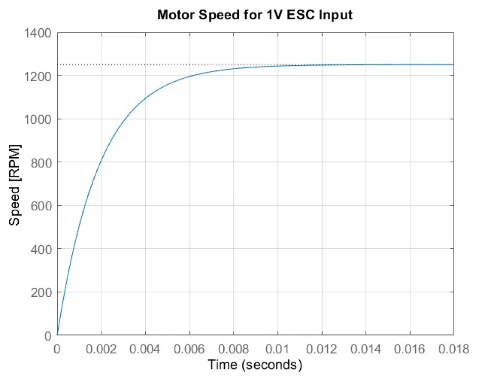Reasonable values for the actuator parameters were selected as follows: motor speed rating k_v = 1250 RPM/V, motor torque constant k_τ = 0.026 Nm/A, motor back EMF constant k_b = 0.002 V/RPM, series resistance R = 0.063 Ω, equivalent friction b_eq = 0.02, equivalent inertia J_eq = 4 × 10⁻⁵ kg·m², supply voltage v = 14.8 V, PWM frequency f_pwm = 16 kHz, and armature inductance $$L=R/(2\sqrt{3}\pi f_{pwm})=3.6\times10^{-7}\,\mathrm{H}$$. Using these values, the actuator’s RPM response to a 1 V input is shown in Figure 2.

Figure 2. Block diagram of the simulation platform.

From the second-order motor dynamics given in (45), the undamped natural frequency is $$\omega_n=\sqrt{(Rb_{eq}+k_bk_\tau)/(LJ_{eq})}$$ = 2996 rad/s. According to [16], the corresponding rise time of the motor response is approximately $$t_{r}\approx3.6/\omega_{n}=1.2$$ ms, which is evident in Figure 3. Based on this, the control loop frequency was set to 200 Hz, allowing 5 ms for the actuators to respond between consecutive commands.

Figure 3. Motor speed response for a 1V input to the electronic speed controller (ESC).

5.3. Sensor Integration Sensors are used to measure state variables. For the quadrotor, GPS, barometer, airspeed sensors, and rate gyros can be used to measure all twelve states, either directly or indirectly. The GPS measures position $$\bar{x},\bar{y}$$, the barometer measures altitude $$\overline{z}$$, and the airspeed sensors measure relative airspeed $$\bar{\dot{x}},\bar{\dot{y}},\bar{\dot{z}}$$. Euler angles and their rates cannot be measured directly; therefore, rate gyro sensors are used to measure body rates $$\bar{\omega}_x,\bar{\omega}_y,\bar{\omega}_z$$, from which the Euler rates $$\bar{\dot{\psi}},\bar{\dot{\theta}},\bar{\dot{\phi}}$$ are estimated using the relationship in (A11). The measured Euler angles $$\bar{\psi},\bar{\theta},\bar{\phi}$$ are then obtained through discrete integration. The measured full state $$\bar{y}=(\bar{x},\bar{y},\bar{z},\bar{\dot{x}},\bar{\dot{y}},\bar{\dot{z}},\bar{\omega}_{x},\bar{\omega}_{y},\bar{\omega}_{z},\bar{\dot{\psi}},\bar{\dot{\theta}},\bar{\dot{\phi}})^{T}$$ is fed into the LQR. Assuming standard deviations of 1 mm, 2 mm, and 3 mm in the x, y, z directions, respectively, the sensor noise covariances are calculated as Q_GP_Sx = 10⁻⁶, Q_GP_Sy = 4 × 10⁻⁶, and Q_Baro = 9 × 10⁻⁶. Asusming a standard deviation of 2 mrad s⁻¹ in the rate gyros the corresponding noise covariance is Q_Gyro = 4 × 10⁻⁶. Similarly, assuming a standard deviation of 5 mm s⁻¹ in air speed sensor, the noise covariance is Q_AirSpeed = 2.5 × 10⁻⁵.

6. LQG Regulator with State Estimation

The LQR is extended to a linear quadratic Gaussian (LQG) regulator by incorporating feedback from Kalman filter estimates. The Kalman filter, using the measured states $$\bar{\mathbf{y}}$$, plant dynamics, and the process and sensor noise covariances, produces state estimates $$\widehat{\mathbf{y}}$$ [17]. The standard Kalman filter, which requires either a linear plant or a fixed linearized model, fails in state estimation because the quadrotor’s high nonlinearity causes the true states to diverge significantly from their estimates when deviating from the hover state. Therefore, the extended Kalman filter (EKF), which uses a state-dependent linearized model $$\begin{aligned}\mathbf{x}(k+1)=\mathbf{x}(k)+\dot{\mathbf{x}}(k)T\end{aligned}$$, is employed [18]. The measured states $$\bar{\mathbf{x}}$$ are connected as inputs to the EKF [19]. The translational and rotational states of the quadrotor can be efficiently estimated using two extended Kalman filters. 6.1. Extended Kalman Filter for Translational State Estimation From (4)–(6), the transitional state vector is $$\mathbf{x}(k)=[x(k),y(k),z(k),\dot{x}(k),\dot{y}(k),\dot{z}(k)]^{T}$$. The first derivatives of this state vector are identified as follows:

```latex\dot{\mathbf{x}}(k)=\begin{bmatrix}\dot{x}_1(k)\\\dot{x}_2(k)\\\dot{x}_3(k)\\\dot{x}_4(k)\\\dot{x}_4(k)\\\dot{x}_6(k)\end{bmatrix}=\begin{bmatrix}x_4(k)\\x_5(k)\\x_6(k)\\(c\psi s\theta c\phi+s\psi s\phi)\frac{F}{m}-\frac{C_x}{m}x_4(k)\\(s\psi s\theta c\phi+c\psi s\phi)\frac{F}{m}-\frac{C_y}{m}x_5(k)\\c\theta c\phi\frac{F}{m}-\frac{C_z}{m}x_6(k)-g\end{bmatrix}```

(46)

Using (46) in the state transition $$\mathbf{x}(k+1)=\mathbf{x}(k)+\dot{\mathbf{x}}(k)T$$, an EKF is constructed to estimate the translational states. 6.2. Extended Kalman Filter for Rotational State Estimation From the rotational dynamics (11)–(13), the rotational state vector is $$\mathbf{x}(k)=(\omega_x,\omega_y,\omega_z)^T$$. The first derivative of these states are identified as follows:

```latex \dot{\mathbf{x}}(k)=\begin{bmatrix}\dot{x}_1(k)\\\dot{x}_2(k)\\\dot{x}_3(k)\end{bmatrix}=\begin{bmatrix}\begin{gathered}\begin{bmatrix}\tau_x-(I_z-I_y)x_2(k)x_3(k)\end{bmatrix}/I_x\\\begin{bmatrix}\tau_y-(I_x-I_z)x_1(k)x_3(k)\end{bmatrix}/I_y\\\begin{bmatrix}\tau_z-(I_y-I_x)x_1(k)x_2(k)\end{bmatrix}/I_z\end{gathered}\end{bmatrix}```

(47)

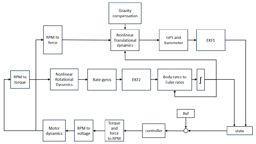
Using (47) in the state transition $$\begin{aligned}\mathbf{x}(k+1)=\mathbf{x}(k)+\dot{\mathbf{x}}(k)T\end{aligned}$$, an EKF is constructed to estimate the rotational states. 6.3. Simulation The simulation is built with the nonlinear quadrotor dynamics under linear quadratic Gaussian control. The simulation framework is built using the subsystems presented in Sections 2–5. Figure 2 illustrates how these subsystems are interconnected to form the complete simulation framework. Bottom layer: The controller compares the reference and actual states to generate the required force and torques. These are then translated into reference motor speeds (RPM), and the corresponding control voltages needed to achieve these RPMs are calculated. The four voltages are then applied as inputs to the motor block, which produces the motor RPMs. Middle layer: The four motor RPMs generate three torques around the quadrotor’s axes, which excite its nonlinear rotational dynamics, resulting in body rates about the three axes. These body rates are measured by the three rate gyro sensors; however, due to sensor noise, EKF2 is used to accurately estimate the body rates. Using the estimated body rates along with the current Euler angles, the Euler rates are computed. Integrating the Euler rates yields the updated Euler angles. Top later: The four RPMs from the motor block produces the force on the quadrotor with respect to the quadrotor frame in its present orientation. This force excites nonlinear translational dynamics, which involved feed-forward gravity compensation and the orientation (Euler angles). Translational dynamics produces linear accelerations of the quadrotor and successive integrations produce linear velocity and position. Linear position is detected by GPS and barometer but the signals are contaminated with noise. Hence the EKF1 is used to estimate linear positions accurately. 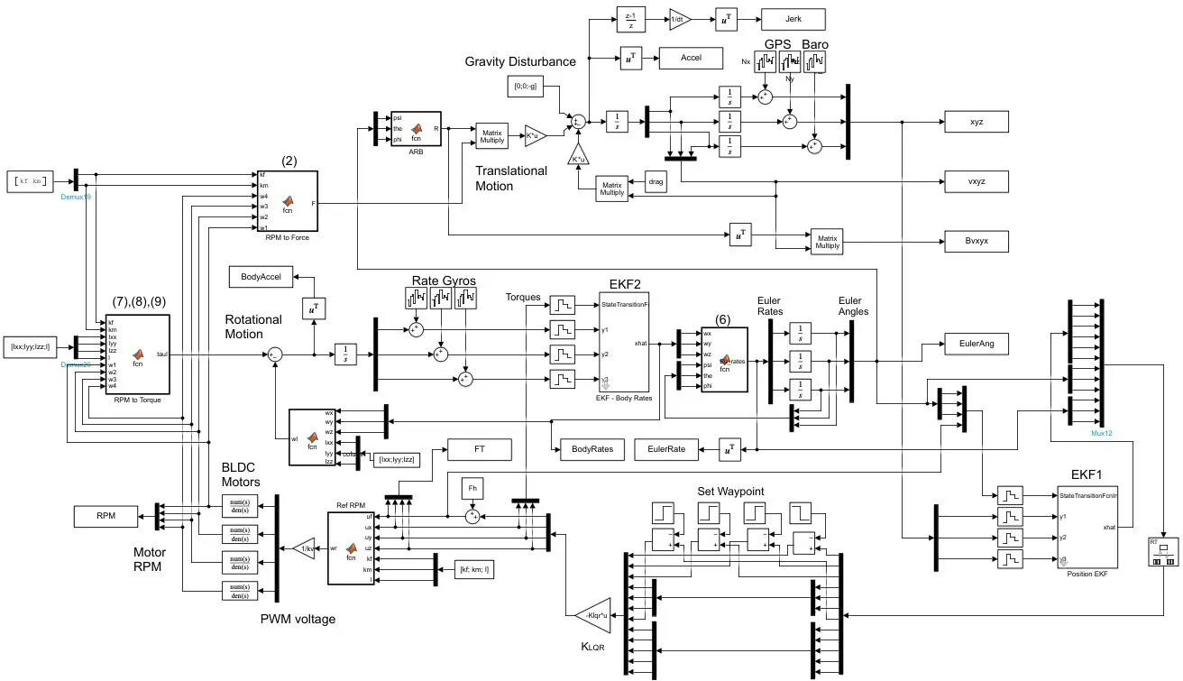The Matlab/Simulink implementation of the simulation framework is illustrated in Figure 4, with subsystems iden- tified as BLDC motors, LQR controller, reference state, EKF1 (translational state estimator), EKF2 (rotational state estimator), and sensors. The reference state is set to x = −4 m, y = 2 m, z = 20 m, and ψ = 0.1π rad.

Figure 4. Matlab Implementation: decoupled dynamics, LQR, two extended Kalman filters, motor dynamics, sensor noise, and feedforward compensation of gravity.

The simulation was successfully executed on two platforms: Acer Nitro 5 with an Intel Core i7 (2.2 GHz), 16 GB RAM, Windows 11, running Matlab-Simulink R2023b; and Lenovo ThinkPad with an Intel Core Ultra 7 (1.4 GHz), 32 GB RAM, Windows 11, running Matlab-Simulink R2024b.

7. Results and Discussion

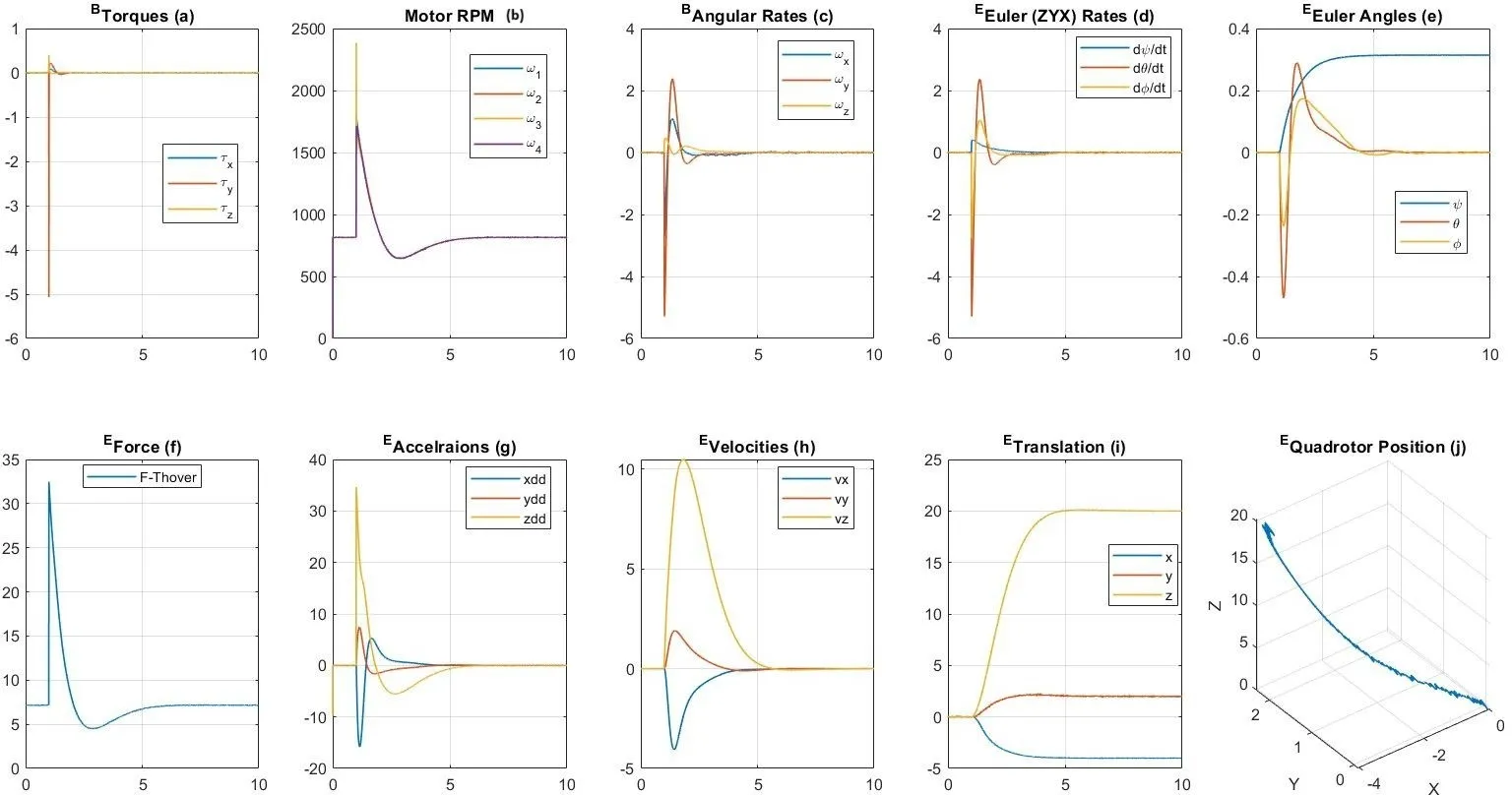
The results are shown in Figure 5. The top row of Figure 5a–e illustrates the rotational motion, while the bottom row Figure 5f–j depicts the translational motion. The quadrotor’s initial state is zero for all variables, and the control input begins at t = 1 s. Figure 5g shows a large positive acceleration in the z-direction, a moderately strong negative acceleration in the x-direction, and a small positive acceleration in the y-direction. These accelerations correspond accurately to the position errors of 20 m, −4 m, and 2 m in the z, x, and y directions, respectively. Figure 5h shows the corresponding linear velocities, and Figure 5i demonstrates that the quadrotor reaches the reference state smoothly and stabilizes there steadily.

Figure 5. Quadrotor flight results under LQG control with state estimates from extended Kalman filters.

Figure 5a shows a large negative torque around the quadrotor’s y-axis at t = 1 s, pushing it along the negative x-direction toward the goal position at x = −4 m. At the same time, Figure 5c displays a sharp negative body rate around the y-axis, followed shortly by a positive y-axis body rate. This sequence allows the quadrotor to start moving in the negative x-direction, then slow down and stop at the reference position. Similarly, Figure 5d shows a corresponding negative pitching followed by positive pitching. Figure 5e illustrates the aggressive pitch control and moderate roll control required to move the quadrotor by −4 m along the x-direction and 2 m along the y-direction. Both pitch and roll angles return to zero at the reference state, while the yaw angle smoothly reaches 0.1π rad. The LQR controller drives the quadrotor to the reference state smoothly, without overshoot or oscillations, in about 5 s. Both EKFs successfully estimate the translational and rotational states despite noise in the GPS, barometer, and rate gyros. Forces, torques, accelerations, velocities, and Euler angles all exhibit smooth variations.

Limitations

This quadrotor simulation is based on the nonlinear quadrotor dynamics under the linear quadratic Gaussian (LQG) ocntrol along with extended Kalman filters for state estimation. Hence, the motion prediction and state estimation remain accurate as long as the system’s nonlinearity is confined within a small range of variation. To satisfy this requirement, the quadrotor’s path should be planned to avoid aggressive roll and pitch maneuvers. The simulation platform has the provision to include and test different controllers for research and educational purposes.

8. Conclusions

This paper presents a thorough analysis of the quadrotor system and its controller design. Translational motion was modeled using Newtonian dynamics, and rotational motion was modeled using Eulerian dynamics. The nonlinear model was simulated in MATLAB/Simulink, while a linearized model was used for the linear quadratic Gaussian (LQG) controller. Gravity was treated as a persistent disturbance, compensated by introducing a hover force as feedforward control. The quadrotor model was linearized at the hover state, and a state-space model was obtained while preserving controllability. A set of sensors including GPS, barometer, airspeed, and rate gyro was included with sensor noise. An extended Kalman filter was used to estimate translational states from the noisy GPS, barometer, and airspeed measure- ments, while another extended Kalman filter estimated body rates from the noisy rate gyro measurements. The estimated states were fed to the LQG controller, and the flight simulation was successfully executed using MATLAB/Simulink on two hardware platforms. This work provides a complete quadrotor simulation platform that can be used by researchers, academics, and students for research, teaching, and self-learning.

Appendix A. XYZ Euler Rotation

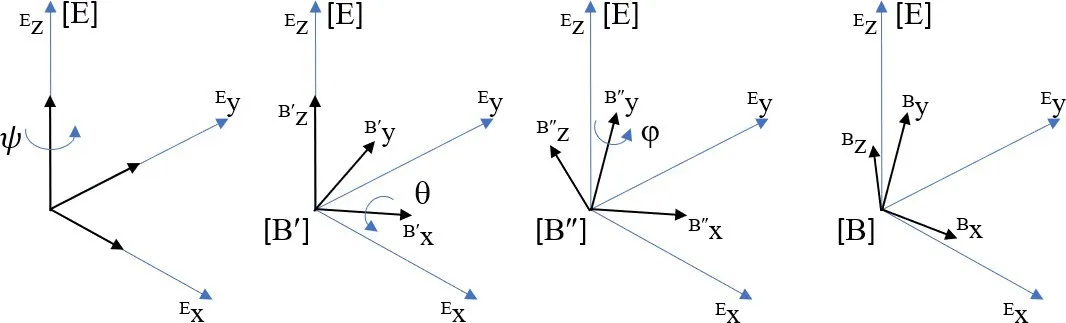
Figure A1 shows a moving frame [B], which is initially coincident with the Earth frame [E], undergoing three successive rotations around its own axes $${}^{B}z\to{}^{B}y\to{}^{B}x$$.

Figure A1. Z-Y-X Euler Rotation.

The intermediate positions of the moving frame after each rotation are denoted by $$[\mathrm{B}^{\prime}],\mathrm{~}[\mathrm{B}^{\prime\prime}]$$ and [B]. The three rotation matrices are given as follows:

```latex R_z(\psi)=\begin{bmatrix}\cos\psi&-\sin\psi&0\\\sin\psi&\cos\psi&0\\0&0&1\end{bmatrix}```

(A1)

```latex R_y(\theta)=\begin{bmatrix}\cos\theta&0&\sin\theta\\0&1&0\\-\sin\phi&0&\cos\phi\end{bmatrix}```

(A2)

```latex R_x(\phi)=\begin{bmatrix}1&0&0\\0&\cos\phi&-\sin\phi\\0&\sin\phi&\cos\phi\end{bmatrix}```

(A3)

In Euler rotation, the orientation of the moving frame [B] with respect to the fixed frame [E] is determined by series multiplication $$_B^ER=R_z(\psi)R_y(\theta)R_x(\phi)$$ which produces the following rotation matrix.

```latex _B^ER=\begin{bmatrix}c\psi c\theta&c\psi s\theta s\theta-s\psi c\theta&c\psi s\theta c\phi+s\psi s\phi\\s\psi c\theta&s\psi s\theta s\phi+c\psi c\phi&s\psi s\theta c\phi-c\psi s\phi\\-s\theta&c\theta s\phi&c\theta c\phi\end{bmatrix}```

(A4)

where S and C are shorthand notations for sin() and cos().

Appendix B. Body Rates and Euler Rates

As shown in Figure A1 Euler rotations $$\psi\mathrm{~}\theta\mathrm{~and~}\phi$$ are referred to the axes $$B_z^{\prime},B_y^{\prime\prime}$$, and B_x. The body rates ^Bω of frame [B] due to Euler angle rates are generated as follows.

```latex {}^{B}\omega=\dot{\phi}B_{x}+\dot{\theta}^{B}B_{y}^{\prime\prime}+\dot{\psi}^{B}B_{z}^{\prime}```

(A5)

where $$^BB_y^{\prime\prime}\mathrm{~and~}^BB_z^{\prime}$$ are the two unit vectors $$B_y^{\prime\prime}$$ and $$B_{z}^{\prime}$$ written with respect to frame [B]. Frame $$\begin{bmatrix}B^{\prime\prime}\end{bmatrix}$$ is related to frame [B] through the rotation matrix $$R_x(\phi)\mathrm{~as~}[B_x^{\prime\prime}B_y^{\prime\prime}B_z^{\prime\prime}]^T=R_x(\phi)[B_xB_yB_z]^T$$, which leads to

```latex B_{y}^{\prime\prime}=\cos\phi B_{y}-\sin\phi B_{z} ```

(A6)

Similarly, frame $$\left[B^{\prime}\right]$$ is related to [B] through $$R_y(\theta)R_x(\phi)$$ as $$[B_x^{\prime}B_y^{\prime}B_z^{\prime}]^T=R_y(\theta)R_x(\phi)[B_xB_yB_z]^T$$, which leads to

```latex \begin{aligned}B_z^{\prime}&=-\sin\theta B_x+\cos\theta\sin\phi B_y+\cos\theta\cos\phi B_z\end{aligned} ```

(A7)

Substitution from (A6) and (A7) into (A5) results

```latex ^B\omega=(\dot{\phi}-s\theta\dot{\psi})B_x+(c\phi\dot{\theta}+c\theta s\phi\dot{\psi})B_y+(c\theta c\phi\dot{\psi}-s\phi\dot{\theta})B_z ```

(A8)

from which the body axis rates are obtained as follows.

```latex \begin{bmatrix}\omega_x\\\omega_y\\\omega_z\end{bmatrix}=\begin{bmatrix}\dot{\phi}-\sin\theta\dot{\psi}\\\cos\phi\dot{\theta}+\cos\theta\sin\phi\dot{\psi}\\\cos\theta\cos\phi\dot{\psi}-\sin\phi\dot{\theta}\end{bmatrix} ```

(A9)

Once rearranged, body rates can be related to Euler rates through the following transformation matrix

```latex \begin{bmatrix}\omega_x\\\omega_y\\\omega_z\end{bmatrix}=\begin{bmatrix}-\sin\theta&0&1\\\cos\theta\sin\phi&\cos\phi&0\\\cos\theta\cos\phi&-\sin\phi&0\end{bmatrix}\begin{bmatrix}\dot{\psi}\\\dot{\theta}\\\dot{\phi}\end{bmatrix}```

(A10)

And, the inverse transformation which is useful to determine Euler angle rates form body rates is as follows.

```latex \begin{bmatrix}\dot{\psi}\\\dot{\theta}\\\dot{\phi}\end{bmatrix}=\begin{bmatrix}0&\sec\theta\sin\phi&\sec\theta\cos\phi\\0&\cos\phi&-\sin\phi\\1&\tan\theta\sin\phi&\tan\theta\cos\phi\end{bmatrix}\begin{bmatrix}\omega_x\\\omega_y\\\omega_z\end{bmatrix}```

(A11)

Acknowledgments

The author acknowledges Lori Leonard, Ronnie Coffman and Richard Cahoon for their assistance and guidance during the preparation of this research at the Dept. of Global Development, College of Agriculture and Life Sciences, Cornell University, Ithaca, USA. Sincere appreciations are extended to the U.S.–Sri Lanka Fulbright Commission (US-SLFC), and the Institute of International Education (IIE), USA for the fascilitation of the Fulbright fellowship of the author at Cornell University, USA.

Ethics Statement

Not applicable.

Informed Consent Statement

Data Availability Statement

Another public repository (GitHub) download link of the proposed MATLAB code is: https://github.com/Rohan- Munasinghe/QuadrotorLQR.

Funding

This research was conducted as part of the Fulbright professional fellowship funded by the U.S. Department of State, Bureau of Educational and Cultural Affairs.

Declaration of Competing Interest

The author declares that there is no known competing financial interests or personal relationships that could have appeared to influence the work reported in this paper.

References

Mahony R, Kumar V, Corke P. Multirotor Aerial Vehicles: Modeling, Estimation, and Control of Quadrotor. IEEE Robot. Autom. Mag. 2012, 19, 20–32. doi:10.1109/MRA.2012.2206474. [Google Scholar]

Khan S, Jaffery MH, Hanif A, Asif MR. Teaching Tool for a Control Systems Laboratory Using a Quadrotor as a Plant in MATLAB. IEEE Trans. Educ. 2017, 60, 249–256. doi:10.1109/TE.2017.2653762. [Google Scholar]

Duc MN, Trong TN, Xuan YS. The quadrotor MAV system using PID control. In Proceedings of the IEEE International Conference on Mechatronics and Automation, Beijing, China, 2–5 August 2015; pp. 506–510. doi:10.1109/ICMA.2015.7237537.

Ma J, Ji R. Fuzzy PID for Quadrotor Space Fixed-Point Position Control. In Proceedings of the Sixth International Conference on Instrumentation & Measurement, Computer, Communication and Control, Harbin, China, 21–23 July 2016; pp. 721–726. doi:10.1109/IMCCC.2016.131.

Faessler M, Falanga D, Scaramuzza D. Thrust Mixing, Saturation, and Body-Rate Control for Accurate Aggressive Quadrotor Flight. IEEE Robot. Autom. Lett. 2017, 2, 476–482. doi:10.1109/LRA.2016.2640362. [Google Scholar]

Kucherov D, Kozub A. Backstepping Algorithm for Controlling of Quadrotor. In Proceedings of the IEEE 6th International Conference on Methods and Systems of Navigation and Motion Control, Kyiv, Ukraine, 20–23 October 2020; pp. 51–55. doi:10.1109/MSNMC50359.2020.9255518.

Zhao W, Liu H, Lewis FL. Data-Driven Fault-Tolerant Control for Attitude Synchronization of Nonlinear Quadrotors. IEEE Trans. Autom. Control 2021, 66, 5584–5591. doi:10.1109/TAC.2021.3053194. [Google Scholar]

Han H, Cheng J, Xi Z, Yao B. Cascade Flight Control of Quadrotors Based on Deep Reinforcement Learning. IEEE Robot. Autom. Lett. 2022, 7, 11134–11141. doi:10.1109/LRA.2022.3196455. [Google Scholar]

Baek J, Kang M. A Synthesized Sliding-Mode Control for Attitude Trajectory Tracking of Quadrotor UAV Systems. IEEE/ASME Trans. Mechatron. 2023, 28, 2189–2199. [Google Scholar]

10.

Choi HD, Kim KS, Shi P, Ahn CK. Adaptive Neuro-Fuzzy Sliding Mode Tracking for Quadrotor UAVs. IEEE Trans. Autom. Sci. Eng. 2025, 22, 16322–16332. [Google Scholar]

11.

Zhu C, Chen J, Iwasaki M, Zhang H. Event-Triggered Deep Learning Control of Quadrotors for Trajectory Tracking. IEEE Trans. Ind. Electron. 2024, 71, 2626–2636. [Google Scholar]

12.

Madebo MM, Abdissa CM, Lemma LN, Negash DS. Robust Tracking Control for Quadrotor UAV With External Disturbances and Uncertainties Using Neural Network Based MRAC. IEEE Access 2024, 12, 36183–36201. [Google Scholar]

13.

Choudry DR. Ch. 11, Modern Control Engineering; Prentice Hall: New Delhi, India, 2005.

14.

Ogata K. Modern Control Engineeing, 5th ed.; Ch. 10-8; Prentice Hall: Upper Saddle River, New Jersey, USA, 2010.

15.

Tariq T, Nahoon M. Constrained Control Allocation Approaches in Trajectory Control of a Quadrotor Under Actuator Saturation. In Proceedings of the 2020 International Conference on Unmanned Aircraft Systems (ICUAS), Athens, Greece, 1–4 September 2020; pp. 131–139.

16.

Munasinghe SR. Classical Control Systems: Design and Implementation; Alpha Science International Ltd.: Oxford, UK, 2012, ISBN 978-1-84265-749-2.

17.

Kalman RE. On the general theory of control systems. IRE Trans. Autom. Control 1959, 4, 110. doi:10.1109/TAC.1959.1104873. [Google Scholar]

18.

Ribeiro I. Kalman and Extended Kalman Filters: Concept, Derivation and Properties; Institute for Systems and Robotics: Lisbon, Portugal, 2004.

19.

Terejanu GA. Extended Kalman Filter Tutorial; University of Buffalo: Buffalo, NY, USA, 2008.