1. Introduction
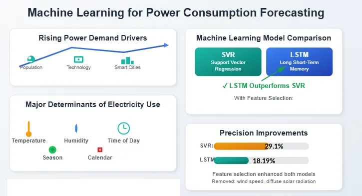
In recent years, there has been a significant increase in electricity demand attributed to factors such as population growth, technological advancements, and the development of smart cities. The growing global dependence on energy permeates various aspects of everyday existence. Effective energy distribution is crucial for minimizing system inefficiencies and return on investment, especially considering the complexities of storing certain energy forms, notably electricity. Matters concerning electrical power are fundamental to societal stability and prosperity. Electricity stands out as a key resource for industrial operations according to economic principles, and precise energy usage forecasting plays a pivotal role in macro-level planning within the energy and industrial domains [
1,
2]. Precise forecasts of future energy consumption are vital for efficient energy distribution planning to maintain a harmonious equilibrium between supply and demand. Erroneous predictions may lead to a disparity between supply and demand, adversely affecting operations, network security, and service standards [
3]. Underestimating energy usage can lead to power outages, which can adversely affect the economy and daily activities. On the other hand, overestimating energy needs can result in unnecessary capacity, leading to wasted resources and a longer return on investment period. It is imperative to ensure that models can accurately predict future energy consumption patterns, particularly when dealing with intricate datasets [
4].
In recent times, Machine Learning (ML) techniques have garnered significant interest owing to their high-performance outcomes across various domains, including healthcare, education, and the energy sector. ML, a subfield of Artificial Intelligence, focuses on developing systems capable of learning and enhancing their performance based on historical data [
5]. Numerous researchers have utilized ML methodologies to construct energy demand forecasting systems. The primary forecasting techniques can be categorized into two main classes. The techniques employed in the first class are based on historical data, utilizing past values of a variable to forecast its future values. Examples of techniques in this class include autoregressive models and time series analysis [
6,
7]. In [
8], the authors developed a system for forecasting electricity demand based on a hybrid approach that combined the Support Vector Regression (SVR) and Empirical Mode Decomposition (EMD) techniques. The Auto-Regressive Integrated Moving Average (ARIMA) approach for forecasting seasonal time series data has been introduced in [
9]. A small-scale agricultural load dataset was used for modelling and forecasting. In [
10], two-time series regression (TSR) models were used for short-term forecasting. Hourly electricity data from South Africa was utilized, covering 2000 to 2010. The first TSR model represents the temperature effects by degree days of heating and cooling. Regression splines were used in the second TSR model to account for the effects of temperature. The first two models were compared in out-of-sample predictions which ranged up to four weeks. Based on empirical findings, the model that incorporates temperature using regression splines gave more accurate estimates. This study in [
11] focused on bridging the knowledge gap in machine learning (ML) techniques for load prediction by employing two forecasting methods: Auto Regressive Integrated Moving Average (ARIMA) and Artificial Neural Network (ANN), and evaluated the efficacy of both methods using Mean Absolute Percentage Error (MAPE).
On the contrary, the second class delves into examining the cause-and-effect relationship between distinct input variables—such as social, economic, and climatic conditions—and energy demand as the resultant output. Regression models and artificial neural networks stand out as the predominant causal methodologies employed to forecast energy consumption [
12,
13,
14]. The author in [
15] introduced a novel approach to energy demand forecasting using Long Short-Term Memory (LSTM) techniques from Deep Neural Networks. The two LSTM models were used: (1) Conventional LSTM and (2) Sequence to Sequence (S2S) architecture based on LSTM. According to the experimental results, the typical LSTM performed well with one-hour resolution data but failed with one-minute resolution data. A proposal for professional energy management has been made in [
15], wherein an IoT-based smart meter is paired with deep extreme machine learning techniques and a support vector machine. Forecasting techniques in the second category currently predict system demand and peak demand values by utilizing weather and historical data on hourly, daily, weekly, monthly, and annual basis. In [
16], the authors developed a sophisticated deep learning algorithm to enhance the accuracy of building energy consumption forecasts. The proposed methodology combined stacked autoencoders (SAEs) with the extreme learning machine (ELM) to leverage their unique characteristics. This proposed method utilized the SAE to extract facets of building energy consumption, while the ELM functioned as a predictor to deliver accurate prediction results. The partial autocorrelation analysis method was utilized to determine the input variables for the extreme deep learning model. In [
17], the authors developed a deep learning system to forecast electricity consumption, taking into account long-term historical dependencies. The cluster analysis was performed on the electricity consumption data for all months to provide seasonally segmented data. Thereafter, a load trend analysis was performed to enhance comprehension of the metadata associated with each cluster. Furthermore, Long Short-Term Memory network multi-input multi-output models were created to forecast electricity consumption utilizing seasonal, daily, and interval data. The author incorporated the concept of moving window-based active learning to improve predictive results in this study. The research in [
18] evaluated and contrasted the two primary short-term load forecasting techniques. The authors first enumerated the prevalent techniques for short-term load forecasting and clarified the principles of Long Short-Term Memory Networks (LSTMs) and Support Vector Machines (SVM). Subsequently, data pre-processing and feature selection were performed in accordance with the characteristics of the electrical load dataset. This report presents the results of a controlled experiment designed to investigate the significance of feature selection. The LSTM and SVM models were employed for one-hour ahead load forecasting and one-day ahead peak and valley load forecasting.
This study focuses on conducting a thorough data analysis and employing feature selection techniques to pinpoint the most influential variables affecting energy demand. The identified features will then be leveraged to develop a precise short-term forecasting system utilizing machine learning methodologies. Thus, the main objectives of this study can be summarized in:
-
-
Extract new features from existing information, such as seasonal and periodical data.
-
-
Conduct an Exploratory Data Analysis (EDA) to identify any hidden features and patterns in the dataset.
-
-
Use multiple linear regression for feature selection.
-
-
Apply two different machine learning models and compare their performance.
-
-
Evaluate the impact of the feature selection step on the performance.
This paper is structured as follows: Section 2 will cover the theoretical framework of this study, including the exploratory data analysis and multiple linear regression. Following that, Section 3 will present the proposed approach. The data set used in this study, and the results are presented in Section 4. Finally, the paper will conclude in Section 5.
2. Theoretical Framework
In this section, the theoretical framework of the proposed method will be explained. The following symbols will be used in the upcoming sections:
-
-
n is the number of samples. As the data considered in this study are taken on an hourly basis. Thus, n represents the hour.
-
-
$$X = \{ x_{i} , i = 0 \ldots . m \}$$ is the set of m collected features (independent variables). The symbol $$x_{i}$$ represents the feature i in the set $$X$$. $$x_{i}$$ can be the temperature, humidity, time, or any other features that may affect electricity demand. $$\overset{-}{x_{i}}$$ represents the mean of the values of the independent variable $$x_{i}$$. $$x_{i , t}$$ represent the variable i at time t.
-
-
$$y_{t}$$ is the values of the dependent variable (electricity demand) at the sample t, and $$\overset{-}{y}$$ is the mean of the values of the dependent variable.
-
-
$$\hat{y_{t}}$$ is the predicted value of the dependent variable at sample t.
2.1. Exploratory Data Analysis
Exploratory Data Analysis (EDA) is a statistical technique that looks for existing hidden patterns and features in a dataset. A variety of statistical visual tools can be applied, including histograms, boxplots, correlation analysis, quantile-quantile (QQ) plots, and many others. EDA is very significant for understanding the relationship between variables before building a forecasting model [
13,
19]. This study will use histogram, scatter, and correlation analysis techniques. Correlation analysis measures the strength of the relationship between two variables without implying causality. Values range from −1 (perfect negative correlation) to 1 (perfect positive correlation), with zero indicating no correlation. Pearson’s correlation coefficient will be used in this study to estimate the relationship between continuous variables.
where $$r_{i}$$ is the correlation coefficient associated with the independent variable $$x_{i}$$ with the dependent variable
y.
2.2. Linear Regression
Linear regression is a supervised ML technique that models the relationship between a dependent variable and one or more independent features, using multiple linear regression (MLR) in this study. It is represented using
Equation (2) [
20]:
where $$\beta_{0}$$ is the intercept (the predicted value of the dependent variable when independent variables equal zero), and $$\beta_{i}$$ are the coefficients associated with the independent variable $$x_{i}$$. It indicates how much the dependent variable will change (increase or decrease) when the independent variable increases by one unit. Using the observed value of the dependent variable $$y_{t}$$, the cost function in MLR can be computed using
Equation (3):
The MLR technique uses a procedure of updating $$\beta_{i}$$ values iteratively to guarantee that the cost function converges to the global minimum values. This procedure entails continuously adjusting the parameters in accordance with the calculated value of the cost function. The coefficient of determination, or
R-Square (
R2), can be used to determine how well a model fits data. It is a statistical indicator of how closely the regression line resembles the real data, and it is given by
Equation (4) [
21]:
Another important outcome of the MLR model is the
p-value. There are three different tests to compute the
p-value for each independent variable $$x_{i}$$. In this study, the two-tailed test is adopted. It is given by
Equation (5) [
22]:
where
cdf is the cumulative distribution function of the test static (T_test), assuming the null hypothesis is true.
T-test is given by
Equation (6):
where
SE is the standard error given by
Equation (7) [
20]:
The null hypothesis, H0 is written as [
19]:
H0: The independent variable
xi has no significant impact on the dependent variable
y.
If the
p-value for
xi is less than 0.01, then, the null hypothesis is rejected and the alternative hypothesis (H1) is adopted. H1 is given by [
23]:
H1: The independent variable
xi has a significant impact on the dependent variable
y.
2.3. MLR for Feature Selection
In this study, MLR is used for feature selection, a process that identifies the most critical features (independent variables) in the model. Reducing the number of variables considered decreases the model’s complexity, improving accuracy. MLR helps determine the significance of each feature’s impact on the dependent variable. Four key factors are considered to identify the most crucial features [
24]: (1) The sign of the coefficient indicates whether a feature has a positive or negative impact on the dependent variable. (2) The magnitude of the coefficient reflects the strength of the feature’s influence. (3) The
p-value shows whether the feature significantly impacts the dependent variable. (4) The model’s
R-squared value demonstrates how well it explains the variation in the dependent variable, with a value of 0.8 indicating that the features in the model account for 80% of the variation.
2.4. Research Questions
The following research questions have been formulated to address the challenges of accurate short-term electricity demand forecasting in this study:
- 1.
-
How can EDA and MLR be used to detect the most influential features impacting short-term electricity demand prediction?
- 2.
-
What is the impact of MLR-based feature selection on the accuracy and performance of ML and DL models for short-term electricity demand prediction?
- 3.
-
How do different ML and DL models, such as SVR and LSTM, perform in predicting short-term electricity demand when they are trained using features selected through the MLR-based feature selection technique?
These questions examine the goals and objectives of this paper by considering how effectively EDA and MLR discover significant characteristics, how feature selection affects model performance, and how different machine learning models compare in terms of accuracy.
3. Method
This paper aims to create an accurate short-term predicting system to generate an accurate estimation of energy consumption value based on weather and historical information. The main goals of this method are to extract new important features, such as chronological and seasonal data from existing information, conduct an EDA to find out any hidden features and patterns in the dataset, employ MLR for feature selection, apply and compare two different ML models, and evaluate the impact of the feature selection step on the performance. The proposed approach is divided into five steps: Gathering and generating data, Data pre-processing and EDA, Features Selection using MLR, ML models, and Performance.
3.1. Gathering and Generating Data
Electricity demand data is typically categorized into three main classes: (1) weather data, including temperature, wind speed, humidity, sky state, and solar radiation; (2) historical electricity consumption data, which includes previous demand values; and (3) household data, such as the area, number of rooms, and the number of people in the household. In this study, household data is not available, particularly when forecasting electricity demand for a region, as opposed to an individual household. Therefore, only the weather and historical consumption data are used. These data can be further enhanced by extracting information such as the season, day of the week, or time of day, which will be incorporated into the dataset to improve electricity demand prediction. More details about the collected dataset are provided in Section 4.1.
3.2. Data Pre-Processing and EDA
The collected data often contains issues like missing values, outliers, and anomalies, requiring pre-processing before applying a machine learning model [
25]. In this study, data preparation includes removing missing values and outliers, followed by applying a standard scaler to the independent variables using the formula [
26]:
where $$x_{i , t , s c a l e d}$$ is the new value of the independent variable $$x_{i , t}$$ after applying a standard scaler, and $$\sigma_{x_{i}}$$ is the standard deviation of the independent variable $$x_{i}$$. After pre-processing, exploratory data analysis (EDA) is performed to identify relationships between variables, utilizing techniques such as Histogram, Boxplot, and Pearson correlation analysis.
3.3. Features Selection Using MLR
In this step, the MLR is used to select the most significant features that greatly impact the electricity demand. This can be done as follows [
27]:
- 1.
-
Divide the dataset into two subsets: $$X$$ which includes all collected data except the historical information about electricity demand, and $$y$$ which includes only the historical values of electricity demand.
- 2.
-
Apply an MLR model by considering $$X$$ as independent and y as dependent variables.
- 3.
-
Display the coefficients $$\beta_{i}$$, $$R - s q u a r e ,$$ and $$p$$_values using Equations (2), (4), and (5). R-square shows how effectively it accounts for variations in the dependent variable. However, $$\beta_{i}$$ shows the importance of each feature $$x_{i }\, \epsilon \,X$$, and $$p$$_values that illustrate if the variable $$x_{i}$$ is significant to the electricity demand or not?
Remove all $$x_{i} \,ϵ \,X$$ with
p-value < 0.01 or with a negligible value of $$β_i$$.
3.4. ML Models
In this paper, two ML models will be applied and compared.
-
-
Support vector regression (SVR) [28]: It is an ML regression technique that has proven to perform well in many industrial applications. It is used to calculate a prediction value of the numerical dependent variable $$y$$ using numerical independent variables $$X$$ at each sample t. For a training set $$T = \{ \left( X_{t} , y_{t} \right) , t = 1 \ldots . n \} $$where $$x i \in R^{m}$$, $$y i \in R$$, m is the number of independent variables, the predicted value of y at sample t can be given by:
where
w represents the vector of coefficients for all features in $$X$$, $$\Phi \left( X_{t} \right)$$ is a kernel function to map features in
X to a vector in feature space, and
b is an intercept. By projecting the original data into a high-dimensional linearly separable space using a kernel function, SVR offers a significant advantage for handling nonlinear processes. Consequently, while creating regression models for nonstationary data, SVR can offer an optimal solution.
-
-
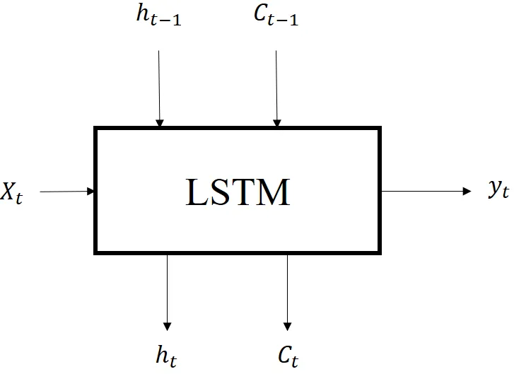
Long Short-Term Memory (LSTM) [29]: It is a type of Neural Network (NN) that overcomes the inconvenience of NN methods by having Long term memory. The LSTM model can be seen as illustrated in .
. LSTM inputs and output at each time step <i>t</i>.
It is composed of the following gates [
30]:
- 1.
-
Forget Gate that can hold or remove information using sigmoid activation function (σ). The output of this function can range from 0 (forget information) to 1 (keep the information).
- 2.
-
Input Gate that expresses the importance of new information carried by the input by performing two activation functions (sigmoid $$\sigma$$ and $$t a n h$$). The role of $$T a n h$$ is to add or subtract information from the cell state, while sigmoid functionality determines whether to keep or reject the information.
- 3.
-
Output gate that delivers the value of the output at each time step using:
where $$\left( W_{f} , W_{i} , W_{o} , W_{c} \right)$$ are the weight matrices and ($$b_{f} , b_{i} , b_{o} , b_{c}$$) are the bias. Note that the weight matrix and the biases are time-independent. In addition, $$f_{t}$$ and $$i_{t}$$ are internal functions in the LSTM and are employed for computing $$c_{t}$$ , $$y_{t} $$ and $$h_{t}$$ at each sample
t.
3.5. Performance
In this paper, five performance metrics will be used to test the proposed approach:
R-square which is explained in Section 2 (
Equation (4)), and mean absolute error (MAE) as given by
Equation (15). It represents the measurement of the typical error magnitude across a set of predictions or forecasts, without considering the direction of the errors [
3]:
The Mean absolute percentage error (MAPE) is given by [
31]:
Based on the MAPE, the accuracy can be computed using:
Therefore, the improvement of the accuracy of the forecasting model due to the MLR in feature selection can be deduced using:
where $$\Delta_{a c c}$$ represents the enhancement of forecast accuracy due to making use of MLR in the feature selection step, $$a c c$$ is the accuracy of the forecasting model with original features, and $$a c c_{w F S}$$ is the accuracy of the forecasting model after using the feature selection based on MLR. In addition, the root mean square error (RMSE) will be considered. It calculates the mean difference between the values that a model predicts and the actual values. It offers an estimate of the accuracy—or how effectively the model can anticipate the desired result:
In this study, the normalized RMSE (NRMSE) is employed. It is given by:
4. Results and Discussion
This section illustrates and discusses the results of applying this approach to a real dataset. The data set is first described, and exploratory data analysis (EDA) is presented to illustrate variable relationships. The performance of the machine learning model is then displayed and compared. Additionally, the advantages of using MLR for feature selection are discussed in terms of forecasting performance.
4.1. Dataset
The dataset used in this study, sourced from [
32], focuses on the city of Tetouan in northern Morocco and its three separate electricity distribution networks. Tetouan spans approximately 10,375 km
2 and had a population of around 550,374 in 2014, with an annual growth rate of 1.96%. Located by the Mediterranean Sea, the city experiences hot, dry summers and mild, rainy winters. The historical data, provided by the Supervisory Control and Data Acquisition System (SCADA), covers the period from 1 January 2017, to 31 December 2017, with readings taken every 10 min [
30]. The dataset includes 52,416 energy consumption samples, each with nine feature columns: Date-Time (day/month/year/hour/minutes), Temperature (in Celsius), Humidity (in g/kg), Wind Speed (in m/s), General Diffuse Flows (in m
3/s), Diffuse Flows (in m
3/s), and Power Consumption for three zones (Zone 1, Zone 2, and Zone 3) recorded in kilowatt-hours (KWh).
4.2. EDA
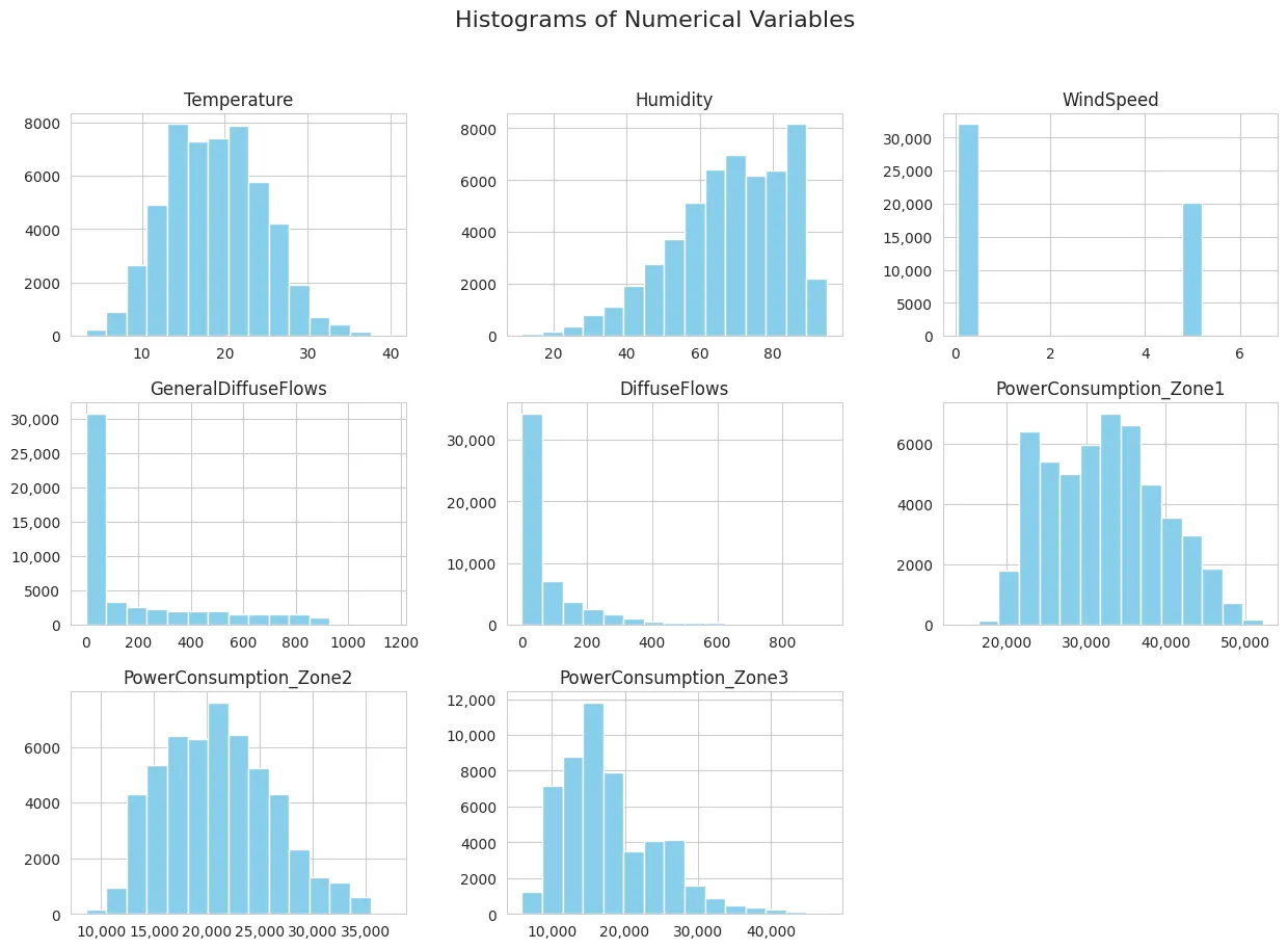
presents histograms of the dataset features, offering insights into their distributional characteristics, such as peak locations, symmetry, skewness, and the presence of outliers. Based on
, several observations can be made: Temperature and power consumption in Zone 2 follow a unimodal and normal distribution, while power consumption in Zone 3 is right-skewed, and humidity is left-skewed. Power consumption in Zone 3 also shows a bimodal distribution, and wind speed is limited to two values. No outliers are present, and a correlation exists between temperature and power consumption across all zones.
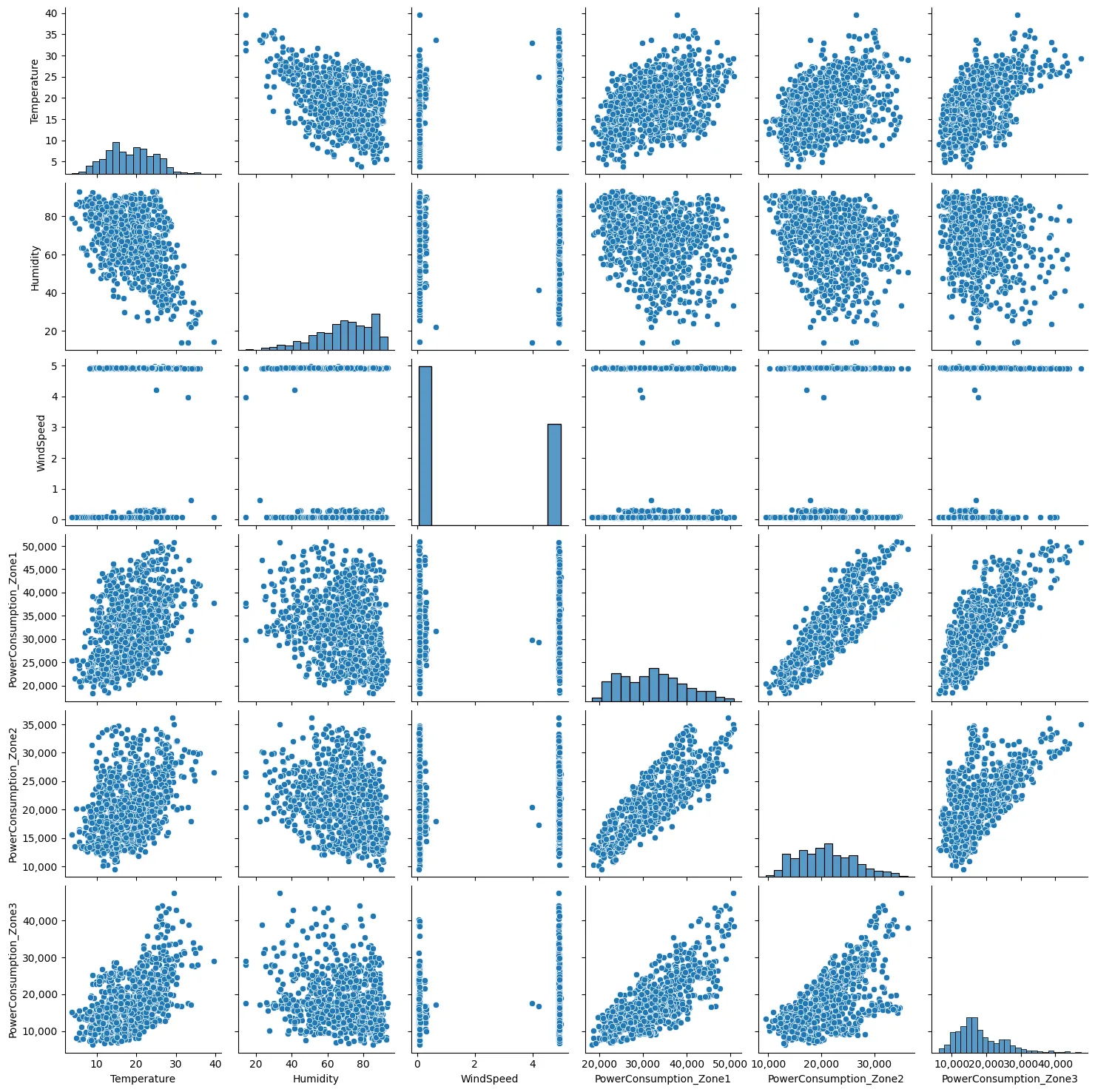
also includes scatter plots of temperature, wind speed, humidity, and power consumption in Zones 1, 2, and 3. Each variable’s values correlate to points on the
x- and
y-axes, respectively. The (
x,
y) coordinates are marked with a dot or another symbol for every pair of variables. There may be hints about the relationship between the two variables in the dot pattern. Based on
, the following points can be concluded:
- 1.
-
There is no correlation between wind spend and others features
- 2.
-
There is a strong relationship between power consumption in zones 1, 2 and 3.
- 3.
-
There is a correlation between temperature and humidity features.
These facts have been confirmed by
and
, which display boxplots of different features.
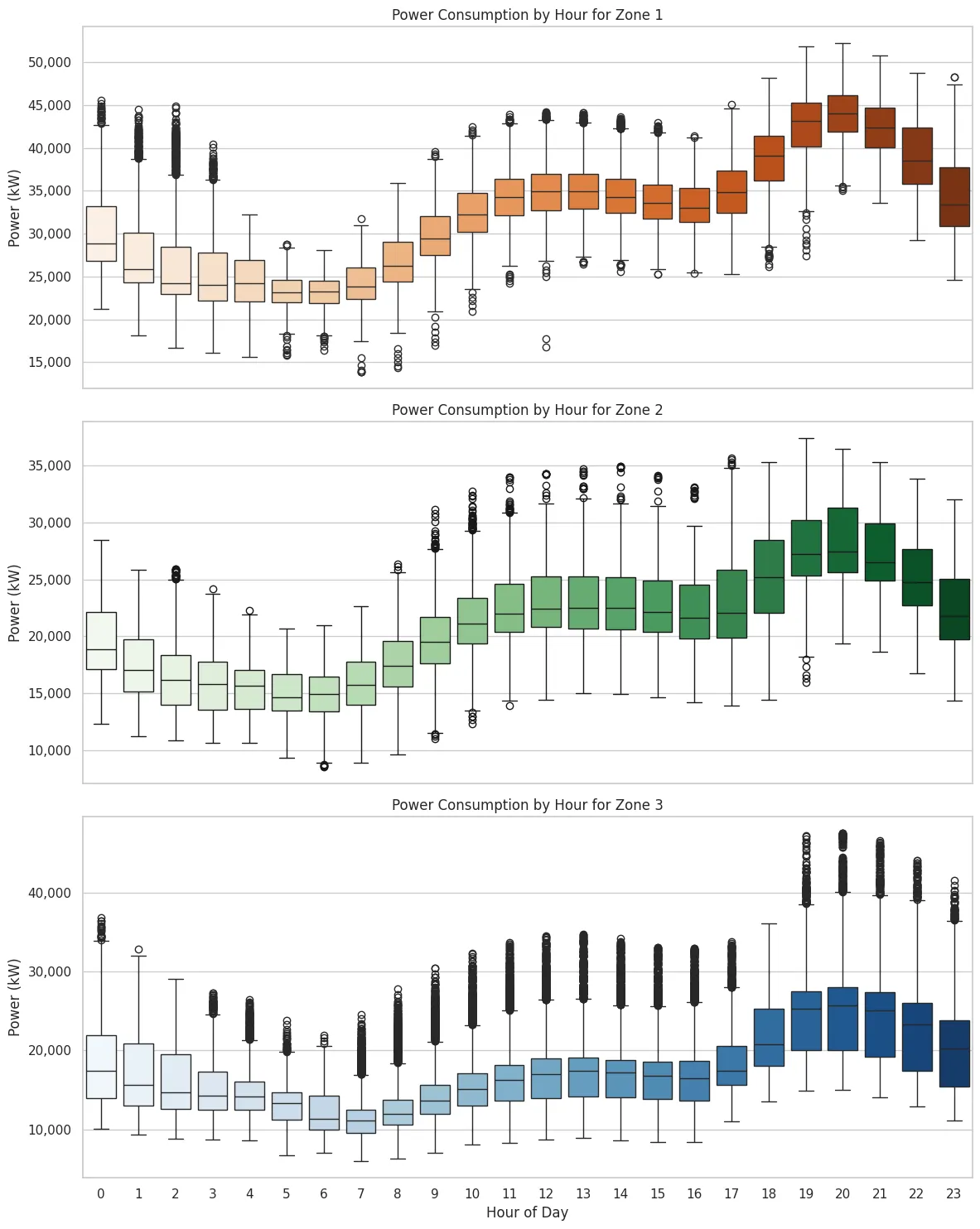
depicts the electricity demand for three zones over a 24-h period. As indicated in the figure, electricity consumption is at its lowest in the morning and peaks at night.
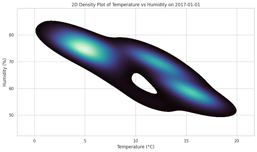
is a 2D density plot that illustrates the distribution of temperature and humidity over the course of one day. The plot shows a clear negative relationship between the two variables: humidity tends to decrease as temperature increases, as shown in the sloping density regions that go from left to right. This figure indicates that higher temperatures mean lower humidity levels. The concentrated high-density areas suggest that this negative correlation remains constant throughout the day. This type of relationship is normal in atmospheric dynamics because warmer air can hold more moisture, with lower relative humidity. Let
X be the set of independent variables, and
y be the dependent variable. In this study,
X ={DateTime, Temperature, Humidity, Wind Speed, General Diffuse Flows, Diffuse Flows in m
3/s}, and
y is the electricity consumption.
. Histogram of dataset features.
From the date and time, other features can be extracted:
- ─
-
Day of the week: this feature can have values between 1 (Monday) and 7 (Sunday)
- ─
-
Hour: it is an integer that has a value between 0 and 23
- ─
-
A month that takes the value 1 for January, and 12 for December.
- ─
-
Seasons: in this study, four seasons are considered: Summer (months 6–9), Autumn (months 9–12), Fall (months 1–3), and Spring (months 3–6).
- ─
-
Humidity: It can be classified as dry or wet. We define moist humidity as the relative air humidity that is 60 percent or higher based on meteorological data. Alternatively, low humidity is assigned.
That
X will be equal to $$X = \{ ‘T e m p e r a t u r e ’ , ‘ H u m i d i t y ’ , ‘ W i n d S p e e d ’ ,‘ G e n e r a l D i f f u s e F l o w s’ ,‘ D i f f u s e F l o w s’ , ‘h o u r’ , ‘ D a y o f w e e k’ , ‘ m o n t h’ ,‘ S e a s o n ’ \}$$ and $$Y = \{ ‘ P o w e r C o n s u m p t i o n \underline{\,\,\,} Z o n e 1 ’ ,‘ P o w e r C o n s u m p t i o n \underline{\,\,\,} Z o n e 2 ’ ,‘ P o w e r C o n s u m p t i o n \underline{\,\,\,} Z o n e 3 ’ \}$$.
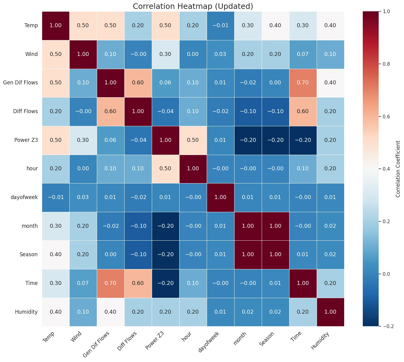
,
and
show the correlation of
X with each variable in
y (Consumption power in zones 1, 2, and 3) computed using
Equation (1). These figures show that:
- -
-
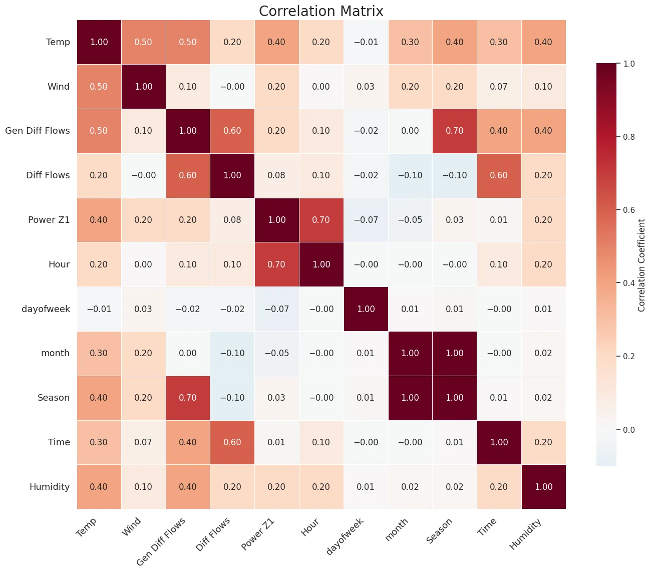
There is a high correlation between electricity consumption in zones 1, 2, and 3 and the variables of hour, month, day, humidity, and temperature.
- -
-
The electricity consumption of zone 2 correlates with the season.
- -
-
The temperature and time correlate with the humidity.
. Scatter for dataset features.
. Electricity consumption for the three zones during one day (Brown: zone 1, Green: zone 2, and Blue: zone 3), with the lowest usage in early morning hours (3–7 a.m.) and a peak in the evening (7–9 p.m.). Power usage gradually increases during the day, and variability is highest during peak hours.
. 2D density plot of temperature and humidity on 1 January 2017, illustrating how temperature and humidity are related to each other: Darker areas show where there are more observations, indicating that humidity tends to go down as the temperature goes up during the day.
. Correlation of different features with electricity consumption of zone 1. Higher correlation values are represented in brown. However, null and negative values are represented in white and grey respectively.
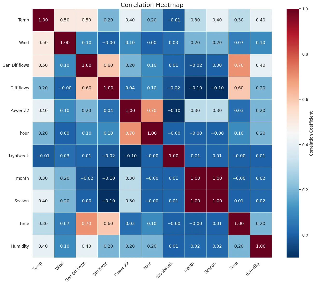
. Correlation of different features with the electricity consumption of zone 2. Higher positive correlation values are represented in red, while negative or weak correlations are shown in blue.
. Correlation of different features with the electricity consumption of zone 3. Higher positive correlation values are represented in red, while negative or weak correlations are shown in blue.
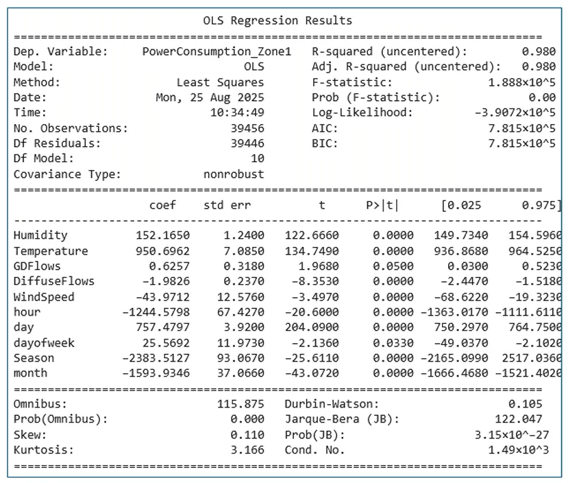
This study uses the MLR to select the most significant features based on
R-square,
p-value, and coefficient magnitude. The dataset is divided into two subsets: 80% for training and 20% for testing.
presents the summary of the MLR model for the electricity consumption of zone 1 using
Equation (2),
Equation (4) and
Equation (5).
In the provided
, the
R-square value is 98%, indicating that the dependent variable explains 98% of the variation in electricity consumption. The features “GeneralDiffuseFlows” and “Day of the week” are not statistically significant (
p-value > 0.01). Additionally, based on the coefficient values $$\beta_{i}$$, it is observed that “Wind speed” and “DiffuseFlows” have a minimal impact on the electricity consumption of zone 1, suggesting that these features can be excluded. Based on
, the MLR model excludes the variables Wind Speed and Diffuse Flows due to their low practical significance. Both variables are statistically significant at the 5% level (
p = 0.000 for Wind Speed and
p = 0.018 for Diffuse Flows); however, the associated coefficients and
t-values indicate a low influence on power consumption compared to other variables such as temperature with a coefficient value of 950.70, or season with a coefficient value of 2338.51. The confidence interval for the variable Diffuse Flows is [−3.718, −0.246], which barely excludes zero. This interval suggests limited robustness in its effect. Moreover, removing these variables enhances the model’s interpretability while preserving its high explanatory power. Consequently, their exclusion is consistent with best practices in model simplification and feature selection. Thus, using
Equation (2), the power consumption in zone 1 can be written as:
Figure 9. Summary of MLR for the electricity consumption of zone 1.
where $$E C$$ is the electricity consumption predicted value, $$x_{1}$$ is the humidity, $$x_{2}$$ is the temperature, $$x_{3}$$ is the time, $$x_{4}$$ is the hour, $$x_{5}$$ is the season and $$x_{6}$$ is the month. The regression coefficients in the above equation show the relative contribution of each variable to electricity consumption. Thus, season (
x₅) and temperature (
x₂) exhibit high positive coefficients, indicating that they are among the most influential factors driving electricity demand. However, time (
x₃) and month (
x₆) present negative coefficients, showing an inverse relationship. Therefore, environmental and temporal features are essential in computing consumption variability, and their combined effect enhances the predictive accuracy of the model.
4.4. ML Prediction Results and Performance
This section will present the results of SVR with a linear kernel and LSTM. The dataset is divided into two subsets: a training set (80%) and a Testing set (20%).
shows the R-square, MAE, MAPE, accuracy, and NRSME ( see Equations (4), (15)–(17) and (20)) for the SVR in both linear and LSTM models.
.
Performance Metrics for SVR with linear kernel and LSTM.
|
SVR with Linear Kernel |
LSTM |
| R-square (%) |
65.9 |
99.7 |
| MAE |
3821.13 |
3272.85 |
| MAPE |
0.105 |
0.013 |
| Accuracy (%) |
89.47 |
98.69 |
| NRSME (%) |
11.3 |
0.84 |
The
R-square value for LSTM is 99.7%, showing its capability to capture almost all variance in the target variable; however, SVR achieves only 65.9%, indicating limited explanatory power. For the absolute error, LSTM achieves a lower MAE (3272.85) compared to SVR (3821.13), confirming its superior prediction precision. The MAPE of the LSTM model (0.013) is lower than that of SVR (0.105), demonstrating that LSTM provides more reliable predictions for demanding electricity, even at different magnitudes.
For the NRMSE, LSTM achieves a remarkably low error of 0.84%, compared to 11.3% for SVR, thus validating its robustness. The prediction accuracy is equal to 98.69% for LSTM. Indeed, LSTM surpasses the SVR model, which achieves an accuracy of 89.47%. These values indicate the effectiveness of LSTM in representing temporal dependencies inherent in electricity demand data.
The results demonstrate that LSTM is more effective for time series prediction tasks such as predicting electricity demand than traditional regression-based models like SVR. This is due to the fact that LSTM uses memory components and gate mechanisms to identify long-term dependencies in sequential data.
shows a comparison between SVR and LSTM with and withput feature selection step. Using
Equation (18), the accuracy improvement of the SVR model and LSTM are equal to:
.
Comparison of performance with and without the features selection step.
|
With Features Selection |
Without Features Selection |
|
SVR |
LSTM |
SVR |
LSTM |
| MAPE |
0.105 |
0.013 |
0.303 |
0.165 |
| Accuracy |
89.47 |
98.69 |
69.3 |
83.5 |
Thus, the feature selection step produces an improvement of 29.1% for the accuracy of the SVR model and 18.19% in the LSTM model for forecasting electricity demand. These results show that the feature selection step improves the performance of both models, especially SVR. The bigger accuracy gain in SVR suggests that it is more sensitive to irrelevant or redundant features, which can degrade its performance. LSTM is better at handling large input spaces on its own, but feature selection still helps significantly by lowering overfitting and improving generalization.
5. Conclusions
As the population grows, technology advances, and smart cities emerge, the demand for electricity increases. To distribute energy effectively, accurate demand prediction is required. This research proposes a novel approach to predicting short-term electricity demand by combining machine learning techniques with exploratory data analysis (EDA) and multiple linear regression (MLR) for feature selection. The suggested method was tested on real data from Tetouan, a city in northern Morocco. Two machine learning models, Support Vector Regression (SVR) and Long Short-Term Memory (LSTM), were applied and compared. EDA found that temperature, humidity, time of day, and season were the most significant factors in predicting electricity usage. The results showed that models trained with MLR-selected features consistently outperform those trained with all the collected data. This approach improves prediction accuracy by 29.1% for SVR and 18.19% for LSTM—while reducing model complexity. The study’s findings emphasize the importance of feature selection in creating reliable forecasting models.
This study shows that combining MLR-based feature selection with advanced machine learning (ML) algorithms enhances the accuracy of electricity demand prediction. The proposed prediction system performs well and yields accurate results under normal conditions. However, the model may deliver less precise outcomes when faced with extreme or unexpected events, such as natural disasters, sudden policy changes, or blackouts. In such cases, the pattern of energy consumption can shift dramatically in ways that are not captured in the training data. Therefore, it is essential to investigate the model’s performance by incorporating real-time data streams and expanding its capabilities to support adaptive learning. This would make the proposed approach more scalable for smart grid applications.
Acknowledgments
We would like to express our sincere gratitude to all those who contributed to the successful completion of this research.
Author Contributions
Conceptualization, G.N., M.N. and O.A.-K.; Methodology, G.N.; Software, G.N. and A.R.; Validation, A.H., G.N., and O.A.-K.; Formal Analysis, O.K. and A.R.; Investigation, G.N. and A. R.; Resources, M.N.; Data Curation, G.N.; Writing—Original Draft Preparation, G.N., and M.N.; Writing—Review & Editing, O.A.-K. and A.R.; Visualization, O.K. and A. R.; Supervision, A.H.; Project Administration, M.N.
Ethics Statement
Not applicable.
Informed Consent Statement
Not applicable.
Data Availability Statement
The dataset used in this study is publicly available and can be accessed freely online.
Funding
This research received no external funding.
Declaration of Competing Interest
The authors declare that they have no known competing financial interests or personal relationships that could have appeared to influence the work reported in this paper.
References
-
1.
Ahmad T, Chen H, Guo Y, Wang J. A comprehensive overview on the data driven and large scale based approaches for forecasting of building energy demand: A review.
Energy Build. 2018,
165, 301–320.
[Google Scholar]
-
2.
Nasserddine G, Nassereddine M, El Arid AA. Internet of things integration in renewable energy systems In Handbook of research on Applications of AI, Digital Twin, and Internet of Things for Sustainable Development; IGI Global: Hershey, PA, USA, 2023; pp. 159–185.
-
3.
Ghalehkhondabi I, Ardjmand E, Weckman GR, Young WA. An overview of energy demand forecasting methods published in 2005–2015.
Energy Syst. 2017,
8, 411–447.
[Google Scholar]
-
4.
Debnath KB, Mourshed M. Forecasting methods in energy planning models. Renew. Sustain.
Energy Rev. 2018,
88, 297–325.
[Google Scholar]
-
5.
El Samad M, Nasserddine G, Kheir A. Introduction to Artificial Intelligence in Artificial Intelligence and Knowledge Processing; CRC Press: Boca Raton, FL, USA, 2023; pp. 1–14.
-
6.
Deb C, Zhang F, Yang J, Lee SE, Shah KW. A review on time series forecasting techniques for building energy consumption. Renew. Sustain.
Energy Rev. 2017,
74, 902–924.
[Google Scholar]
-
7.
Shih S, Sun F, Lee H. Temporal pattern attention for multivariate time series forecasting.
Mach. Learn. 2019,
108, 1421–1441.
[Google Scholar]
-
8.
Yaslan Y, Bican B. Empirical mode decomposition based denoising method with support vector regression for time series prediction: A case study for electricity load forecasting.
Measurement 2017,
103, 52–61.
[Google Scholar]
-
9.
Noureen S, Atique S, Roy V, Bayne S. Analysis and application of seasonal ARIMA model in energy demand forecasting: A case study of small scale agricultural load. In Proceedings of the 2019 IEEE 62nd International Midwest Symposium on Circuits and Systems (MWSCAS), Dallas, TX, USA, 4–7 August 2019.
-
10.
Román-Portabales A, López-Nores M, Pazos-Arias JJ. Systematic review of electricity demand forecast using ANN-based machine learning algorithms.
Sensors 2021,
21, 4544.
[Google Scholar]
-
11.
Tarmanini C, Sarma N, Gezegin C, Ozgonenel O. Short term load forecasting based on ARIMA and ANN approaches.
Energy Rep. 2023,
9, 550–557.
[Google Scholar]
-
12.
Unutmaz YE, Demirci A, Tercan SM, Yumurtaci R. Electrical energy demand forecasting using artificial neural network. In Proceedings of the 2021 3rd International Congress on Human-Computer Interaction, Optimization and Robotic Applications (HORA), Ankara, Turkey, 11–13 June 2021.
-
13.
Bedi J, Toshniwal D. Deep learning framework to forecast electricity demand.
Appl. Energy 2019,
238, 1312–1326.
[Google Scholar]
-
14.
del Real AJ, Dorado F, Durán J. Energy demand forecasting using deep learning: applications for the French grid.
Energies 2020,
13, 2242.
[Google Scholar]
-
15.
Marino DL, Amarasinghe K, Manic M. Building energy load forecasting using deep neural networks. In Proceedings of the IECON 2016 - 42nd Annual Conference of the IEEE Industrial Electronics Society, Florence, Italy, 23–26 October 2016.
-
16.
Ghazal TM. Energy demand forecasting using fused machine learning approaches.
Intell. Autom. Soft. Comput. 2022,
31, 539–553.
[Google Scholar]
-
17.
Li C, Ding Z, Zhao D, Yi J, Zhang G. Building energy consumption prediction: An extreme deep learning approach.
Energies 2017,
10, 1525.
[Google Scholar]
-
18.
Pallonetto F, Jin C, Mangina E. Forecast electricity demand in commercial building with machine learning models to enable demand response programs.
Energy AI 2022,
7, 100121.
[Google Scholar]
-
19.
Komorowski M, Marshall DC, Salciccioli JD, Crutain Y. Exploratory data analysis. In Secondary Analysis of Electronic Health Records; Springer: Berlin/Heidelberg, Germany, 2016.
-
20.
Mirkin B. Core Data Analysis: Summarization, Correlation, and Visualization; Springer International Publishing: Cham, Switzerland, 2019.
-
21.
Pandis N. Linear regression.
Am. J. Orthod. Dentofac. Orthop. 2016,
149, 431–434.
[Google Scholar]
-
22.
Darlington RB, Hayes AF. Regression Analysis and Linear Models: Concepts, Applications, and Implementation; Guilford Publications: New York, NY, USA, 2016.
-
23.
Andrade C. The P value and statistical significance: misunderstandings, explanations, challenges, and alternatives.
Indian J. Psychol. Med. 2019,
41, 210–215.
[Google Scholar]
-
24.
Hasan MA, Hasan MK, Mottalib MA. Linear regression–based feature selection for microarray data classification.
Int. J. Data Min. Bioinform. 2015,
11, 167–179.
[Google Scholar]
-
25.
Nasserddine G, Amal A. Decision-making systems In Encyclopedia of Data Science and Machine Learning; IGI Global Scientific Publishing: Hershey, PA, USA, 2023; pp. 1391–1407.
-
26.
García S, Luengo J, Herrera F. Data Preprocessing in Data Mining; Springer International Publishing: Cham, Switzerland, 2015.
-
27.
Guo Y, Wang W, Wang X. A robust linear regression feature selection method for data sets with unknown noise.
IEEE Trans. Knowl. Data Eng. 2021,
35, 31–44.
[Google Scholar]
-
28.
Nassreddine G, El Arid A, Nassereddine M, Al-Khatib O, Arram A, El Abed A. Enhancing the Efficacy of Short-Term Prediction Models for Solar Photovoltaic Systems: An Influence Examination of Chronological and Meteorological Factors.
IEEE Access 2025,
13, 66787–66808.
[Google Scholar]
-
29.
Yu Y, Si X, Hu C, Zhang J. A review of recurrent neural networks: LSTM cells and network architectures.
Neural Comput. 2019,
31, 1235–1270.
[Google Scholar]
-
30.
Hrnjica B, Mehr AD. Energy demand forecasting using deep learning In Smart Cities Performability, Cognition, & Security; Springer: Berlin, Germany, 2019; pp. 71–104.
-
31.
Eseye AT, Lehtonen M, Tukia T, Uimonen S, Millar RJ. Machine learning based integrated feature selection approach for improved electricity demand forecasting in decentralized energy systems.
IEEE Access 2019,
7, 91463–91475.
[Google Scholar]
-
32.
Fedesoriano. Electric Power Consumption. Available online: https://www.kaggle.com/datasets/fedesoriano/electric-power-consumption (accessed on 2 June 2024).