1. Introduction
1.1. Background
With the increasing depletion of fossil fuels and excessive carbon emissions from energy consumption, renewable energy resources, such as wind and solar energy, have been rapidly developing in recent years. As an important form of wind energy utilization, wind power generation has attracted much attention because of its potential for large-scale development and high-efficiency utilization [
1]. In accordance with the Global Wind Energy Council [
2], the global newly installed capacity of wind power reached a record high of 117 GW in 2024, and the cumulative installed capacity reached 1136 GW. However, wind power generation has intermittency and volatility because the weather greatly influences it. With the large-scale on-grid connection of wind power, the intermittency and volatility adversely affect the controllability of power generation and the safe and economic operation of power systems [
3]. Therefore, high-precision wind power prediction becomes a fundamental condition for large-scale integration of wind power and plays an important role in the safe and economic operation of power systems [
4,
5]. Furthermore, forecast results can be used in the energy market to influence the profits of wind farms [
6,
7].
1.2. Literature Review
1.2.1. Hybrid Methods for Wind Power Prediction
Many approaches have been proposed for wind power prediction. These approaches can be divided into four categories, namely physical, statistical, artificial intelligence, and hybrid methods [
8]. Hybrid methods have attracted considerable attention because the advantages of various models can be combined to improve predictive accuracy. In literature, hybrid methods are divided into two subcategories: stacking-based methods and weight-based methods [
9]. In stacking-based methods, various models are combined in series, that is, the output of one model is input into another model as a feature extracted. In a study [
10], the gated recurrent unit (GRU) and convolutional neural network (CNN) were combined to extract temporal features and spatial features of a wind farm, respectively. In another study [
11], the CNN and radial basis function neural network with a double Gaussian function were used to form a hybrid model. Furthermore, some sequence decomposition methods have been introduced to stacking-based models, such as wavelet transform [
12], empirical mode decomposition [
13], and local mean decomposition [
14]. These methods can capture the characteristics of several different time scales in the original nonstationary sequence and decompose it to obtain a set of stationary subsequences. However, the aforementioned models still function as individual predictors, but they may have some drawbacks, such as overfitting, incorrect model specifications, and relative sensitivity to initial parameters [
15]. These problems can be solved by using the ensemble technique [
16]. In the weight-based methods, the ensemble technique can be used to combine the results of individual predictors using the weight allocation strategy. In [
17], a hybrid wind speed forecasting model that combines three basic models was proposed. In [
18], the wind power was predicted by combining the least square support vector machine, extreme learning machine (ELM), and the variance strategy to determine the corresponding weights. including overfitting, incorrect model specifications, and high sensitivity to initial parameters
1.2.2. Multi-Step Prediction
Most existing studies have focused on single-step prediction. With the integration of high penetration wind power into power systems, the limited information obtained from single-step prediction cannot satisfy the requirements of wind power dispatching [
19]. Multi-step predictions have a smaller demand for real-time data and can provide more information than single-step predictions [
20]. Furthermore, the forecast results are highly specific. Therefore, researchers are shifting their focus to multi-step prediction. However, in multi-step prediction, the global error of the prediction interval should be considered. Moreover, a greater number of prediction steps can result in lower accuracies [
21]. Generally, providing a forecast wind power sequence with high accuracy is difficult.
Research on multi-step prediction can be classified into three categories: recursive, direct, and multi-input multi-output (MIMO) methods [
22]. The first two methods are developed based on the single-step prediction model, whereas a multi-output model is established in the MIMO method. In the recursive method, a single-step prediction model is established. Next, the forecast value at the previous step is used to predict the next step value. Multi-step forecast values can be obtained through iterations. In this method, only one prediction model should be optimized, and the training of the model is the same as that in single-step prediction. The obvious disadvantage of this method is error accumulation. The errors in the last few steps may reach an unbearable level with the increase in prediction steps.
The direct method was developed for multi-step prediction to avoid cumulative errors caused by multiple iterations in the recursive method. In the direct method, a set of single-step prediction models is built, corresponding to the prediction task of each time step, and the number of prediction models is equal to the number of prediction steps [
23]. In general, the direct method becomes highly complex with increased prediction steps. Although the cumulative error becomes lower than that of the recursive method, the error at the subsequent step is still higher than at the previous step because only the wind power at the nearest time points is highly correlated with the current observed wind power. The direct method splits multi-step prediction into independent single-step prediction tasks, which indicates that prediction profiles may be incoherent and models cannot consider the temporal correlation between different step-ahead predictions [
24]. The MIMO method can generate multi-step outputs in a single operation, and no recursive process is required.
The MIMO method can generate multi-step outputs in a single operation, and no recursive process is required [
25], which is a widely used strategy in multi-step prediction research. The MIMO reduces complexity and cumulative error, and the overall performance is superior to that of the recursive and direct methods. However, optimizing such a model with multiple outputs is challenging. In [
26], Bao et al. proposed a multi-output support vector regression (MSVR). They verified its superior performance over normal SVR with a recursive strategy in a multi-step time-series prediction. However, the MSVR model ignored the relevance between prediction tasks and the temporal dependency between inputs.
The limitations of the MIMO method can be addressed using two methods. In one method, the recurrent neural network (RNN) models are used to capture temporal correlations among input variables accurately. In the other method, novel inference frameworks are introduced to eliminate the accumulation of errors and consider the correlations among successive prediction tasks. Considering the similarity between multi-step prediction and machine translation tasks in natural language processing, some sequence-to-sequence (S2S) models with encoder–decoder inference architecture used widely in machine translation have been introduced in wind power multi-step prediction. Under the encoder–decoder architecture, the encoder extracts the feature information of the input sequence and outputs an encoded vector. The decoder decodes the encoded vector to obtain the translation sentence or predictive wind power sequence. In theory, the recurrent neural network is suitable as the core network to form an encoder–decoder model. A study [
27] proposed an encoder–decoder-based prediction model using long short-term memory (LSTM) as a core network layer. This model could mine information only from a fixed-length representation of input variables. In [
28], Neshat et al. used a bidirectional version of the LSTM model to achieve the purpose of bidirectional reading. Compared with the model proposed in [
27], Niu et al. replaced the LSTM with GRU. They proposed an attention-based feature selection method to enhance the performance of the encoder–decoder architecture [
24]. Similar to [
28], inspired by the performance of bidirectional GRU (Bi-GRU), Wang et al. proposed the S2S Bi-GRU model based on an attention mechanism and improved predictive accuracy [
29].
However, the encoder–decoder model based on the RNN supports only serial operation, and computational efficiency becomes low when the input sequence becomes longer or the prediction steps increase. Furthermore, the RNN cannot accurately capture the long-term dependency of the sequence. To address the problem of the RNN-based encoder–decoder model, Vaswani et al. used a self-attention mechanism to establish a model named Transformer [
30], which can extract mixed dependency information of all kinds of sequence scales and establish the relationship between the input and output. The Transformer outperformed other models on translation tasks in multiple languages in terms of precision and computational speed. Inspired by the Transformer, this model has been applied to time-series prediction tasks. Wang et al. [
31] proposed a multi-modal multi-task transformer network model for wind power prediction. In this model, many Transformer modules were used to extract information of input variables. Zhou et al. [
32] proposed a model named Informer to enhance the computational performance of long-sequence time-series prediction. The Informer was applied to the transformer oil temperature prediction task. In [
33], Yang et al. combined multi-head attention (MHA) with multivariate variational mode decomposition, elastic net, CNN, and bidirectional LSTM to predict the outputs of a wind farm.
1.3. Contributions and Organization
To address the aforementioned challenges, a novel hybrid model based on the encoder–decoder architecture was proposed for multi-step ultra-short-term power prediction of wind farms. This hybrid model combines Bi-GRU, MHA mechanism, and ensemble technique. Compared with similar research, the core contributions of this paper are summarized below.
- 1.
-
A novel hybrid encoder–decoder prediction model was proposed based on Bi-GRU and MHA. The Bi-GRU was used in the encoder to extract complex temporal dependency among input variables. The decoder used the MHA mechanism to efficiently and accurately mine information from the encoding vector to obtain the forecast wind power sequence. Compared with the conventional encoder–decoder model based on the RNN, the MHA can identify features contributing to the output and improve predictive accuracy.
- 2.
-
An ensemble forecast method that combines the proposed prediction model was developed. According to the evaluation performance of each predictor, the ensemble result can be obtained by integrating the forecast results of the individual predictors to reduce the uncertainty of individual prediction results and enhance forecast accuracy.
- 3.
-
The proposed model can achieve multi-step wind power prediction with high accuracy, and the forecast results can provide more information for the safe and economic dispatching of wind power than those with single-step prediction.
In the rest of this paper, Section 2 introduces the encoder–decoder architecture for multi-step prediction, Section 3 elaborates on the multi-step prediction model, and Section 4 details the implementation of the proposed prediction model combining with the ensemble technique. Section 5 presents numerical results. Finally, Section 6 presents the conclusions of this paper.
2. Encoder–Decoder Architecture for Multi-Step Prediction
The result of conventional single-step wind power prediction is a value that represents the output at a certain future time point. Unlike single-step prediction, multi-step prediction provides wind power sequence in a certain future period. The length of the sequence is defined as the prediction steps.
Therefore, the multi-step wind power prediction is an S2S prediction problem. The encoder–decoder architecture is an effective method for solving this problem, which exhibits excellent performance in natural language processing and time-series prediction. The encoder–decoder model generally consists of two networks. The encoder first extracts the feature information of the input sequence and represents it as an encoded vector. The process is expressed as
where
Xen,t is the output of the encoder, that is, encoded vector,
Xt and
Wt are the input historical features and future features at time
t, respectively;
fencoder(
·) and
θ denote the implicit function and parameters of the encoder, respectively; and
p and
q are the length of historical and future information sequence, respectively.
After obtaining the encoded vector from the encoder, the decoder starts to function and mine dependency between the input and output. Two strategies are used to return the forecast wind power sequence. The original strategy used a recursive method similar to machine translation. This process is expressed as
where
ŷt+i $$\hat{y}_{t + i}$$ represents the output at time
t+i, that is, the forecast value at the
i-th time step;
fdecoder(
·) and
ρ represent the implicit function and parameters of the decoder, respectively; and
s is the set number of prediction steps. After
s iterations described in
Equation (2), the final forecast wind power sequence $$\hat{\bm{y}} = \left[ \hat{y}_{t + 1} , \hat{y}_{t + 2} , . . . , \hat{y}_{t + s} \right]$$ can be obtained.
In addition to the recursive method, the decoder can use the direct generative method to implement multi-step forecast. In this method, the forecast sequence can be obtained without recursive processes, which is expressed as follows:
The following aspects hinder efficient encoder–decoder modeling. One aspect is to develop the functions of encoder and decoder, that is,
fencoder(
·) and
fdecoder(
·). The other aspect is to optimize the parameters of the encoder and decoder, that is,
θ and
ρ. The details of addressing these challenges are introduced in the next sections.
3. Multi-Step Wind Power Prediction Model Based on Bi-GRU and MHA
3.1. Input Information
The input of the proposed model contains two parts, one part is historical information, and the other includes future information, as displayed in
. The historical information includes wind power, wind speed, and wind direction at the historical time. We used vector
Xt−i to represent this information at a certain time as follows:
where
WPt−i, WSt−i, and WDt−i represent historical wind power, wind speed, and wind direction at time
t − i, respectively. When using
p time lag windows of input variables,
p vectors can be spliced together to form an input matrix $$\bm{X}_{i n , t} = \left[ \bm{X}_{t - p + 1} , \bm{X}_{t - p + 2} , . . . , \bm{X}_{t} \right] \in R^{3 \times p}$$.
Future information is obtained through numerical weather prediction (NWP) of a certain wind farm, including the prediction of wind speed and wind direction in the future. Vector
Wt+i was used to represent this information at a certain time as follows:
where
PWSt+i, and
PWDt+i represent the prediction speed and direction of wind at time
t + i, respectively. Similarly,
q time windows of input variables can be used to form input matrix $$\bm{W}_{i n , t} = \left[ \bm{W}_{t + 1} , \bm{W}_{t + 2} , . . . , \bm{W}_{t + q} \right] \in R^{2 \times q}$$. Here,
q is a parameter determined by the temporal resolution and prediction duration of NWP.
. Input matrices and output for the proposed model.
3.2.1. Bi-GRU Network
The GRU is an improved version of the RNN proposed in 2014 [
34]. Similar to LSTM, another variant of the RNN, GRU incorporates the gated mechanism. However, in the mechanism, one gate and one hidden state variable are reduced compared with LSTM, and its structure is simplified. This structure enhances computing efficiency and is especially suitable for processing a large amount of data and long-term time-sequence data. The inner structure of the GRU cell is illustrated in
.
Two gates (
i.e., the reset gate and update gate) are used in the GRU cell, and their forward operations are defined as follows:
where
rt represents the output of reset gate,
ut represents the output of update gate; σ(·) is the sigmoid activation function;
xt denotes the input at time
t ;
ht−1 denotes the hidden state at time
t − 1;
wxr,
whr,
wxu, and
whu are corresponding weight matrices; and
br and
bu are the biases of the reset gate and update gate, respectively.
The recurrent variable in the GRU cell is the hidden state, and the operations are defined as follows:
where $$\overset{\sim}{\bm{h}}_{t}$$ represents the temporary state of the hidden state,
ht represents the current hidden state, $$\odot $$ represents the element-wise multiplication,
tanh(
·) represents the hyperbolic tangent activation function,
wxh and
whh are corresponding weight matrices, and
bh is the bias of the hidden state.
The expressions of sigmoid activation function and tanh activation function are defined as follows:
The conventional GRU network transfers information along the front-to-back order in the temporal dimension. Therefore, the temporal features in the forward direction can be extracted. To completely extract the temporal features in the wind power sequence and enhance network capability, we used Bi-GRU, which adds a layer to the conventional GRU to transmit information in the reverse order of time. The structures of the conventional GRU network and Bi-GRU network are illustrated in
. Assuming that the two layers transmit information in time order and reverse time order, and the hidden states of these two layers at time
t are $$\bm{h}_{t}^{\left( 1 \right)}$$ and $$\bm{h}_{t}^{\left( 2 \right)}$$, respectively, the final hidden state can be expressed as follows:
where $$f_{G R U} \left( \cdot \right)$$ represents the gated operation of GRU and $$\oplus$$ represents the concatenation operation of vectors.
. Inner structure of the GRU cell.
. Structure of different GRU networks: (<b>a</b>) conventional GRU; and (<b>b</b>) Bi-GRU.
3.2.2. MHA Mechanism
The attention mechanism is applied in machine learning to capture crucial information in the input sequence data. An attention function describes the connection between a query vector and a set of key-value vector pairs. Given
Nk key-value vector pairs and a query vector
q, the keys with dimension of
dk and values with dimension of
dv are packed into matrices $$\bm{K} = \left[ \bm{k}_{1} , \bm{k}_{2} , . . . , \bm{k}_{N_{k}} \right]^{\mathrm{T}}$$ and $$\bm{V} = \left[ \bm{v}_{1} , \bm{v}_{2} , . . . , \bm{v}_{N_{k}} \right]^{\mathrm{T}}$$. First, the similarity between the query and all keys is calculated using functions such as dot product and additive. The softmax function is then used to normalize results from the similarity calculating process. In this way, the normalized weight of each key-value pair, the attention distribution, can be obtained. The process of calculating the attention distribution can be expressed as follows:
where
αi denotes the weight of key-value pair
i, and
sim(
·) represents the function of calculating the similarity between the query and key.
The final output of the attention function is the sum of the products of all values and their corresponding weights. Thus, all inputs are no longer equally important to the output. Thus, the input with higher correlation with the output has higher proportion in the output. The calculation of the output of the attention function can be expressed as follows:
In practice, a set of queries is added to calculate attention and packed into a matrix $$\bm{Q} = \left[ \bm{q}_{1} , \bm{q}_{2} , . . . , \bm{q}_{N_{q}} \right]^{T}$$. When using dot product as a function
sim(
·) to calculate the similarity, the dot-product attention calculation in
Equation (15) and
Equation (16) can be described by matrix multiplication, as follows:
where
Dattn(
·) represents the function of the dot-product attention mechanism; $$\bm{Q} \in R^{N_{q} \times d_{k}}$$, $$\bm{K} \in R^{N_{k} \times d_{k}}$$, and $$\bm{V} \in R^{N_{k} \times d_{v}}$$are inputs of the attention mechanism;
Nk and
Nq are the numbers of keys and queries; and $$\sqrt{d_{k}}$$ is an adjustment scale factor to prevent the inner dot-product value from becoming too large.
Compared with the single dot-product attention, MHA allows the model to jointly attend to information from different representation subspaces at distinct positions [
28]. As displayed in
, queries, keys, and values with dimension of
dm, are linearly projected to
dk,
dk, and
dv dimensions through different linear projections, respectively. The dot-product attention for the new group of queries, keys, and values is calculated using
Equation (17). Projection and attention calculation are repeated several times. This process is called multi-head and expressed as follows:
where $$\bm{h} \bm{e} \bm{a} \bm{d}_{i} \in R^{N_{q} \times d_{v}}$$ represents the output of the
i-th head of attention mechanism;
Nh is the number of heads; and $$\bm{W}_{i}^{Q} \in R^{d_{m} \times d_{k}}$$, $$\bm{W}_{i}^{K} \in R^{d_{m} \times d_{k}}$$, and $$\bm{W}_{i}^{V} \in R^{d_{m} \times d_{v}}$$ are the parameter matrices of projections.
The outputs are concatenated in the dimension of
dv and projected to the original dimension of
dm, resulting in the final output of the MHA. The calculation process of MHA is as follows:
where
MHA(
·) represents the function of the MHA mechanism,
Concat(
·) represents the concatenation operation of matrices, and $$\bm{W}^{O} \in R^{N_{h} d_{v} \times d_{m}}$$is the parameter matrix of the output projection.
. Structure of the multi-head attention mechanism.
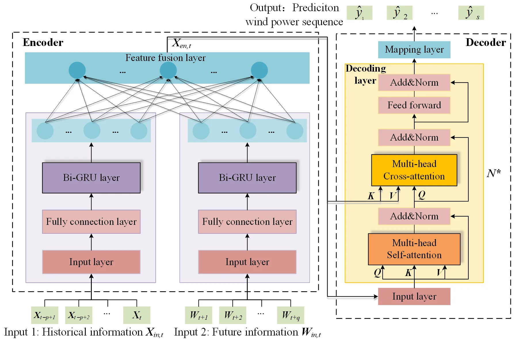
The proposed multi-step wind power prediction model based on Bi-GRU and MHA is illustrated in
, which belongs to a hybrid encoder–decoder architecture.
Encoder: To comprehensively utilize the historical information features and future information features of a wind farm, the encoder contains two submodules, each of which consists of the input layer, a fully connected layer, and Bi-GRU layer. The two modules process the input information introduced in Section 3.1 and output different hidden states containing key temporal features of the corresponding input information. These temporal features extracted by two Bi-GRU-based modules are passed through a feature fusion layer to realize feature fusion to obtain the final encoded vector sequence
Xen,t.
Decoder: Unlike the conventional encoder–decoder model based on the RNN, we replaced the RNN in the decoder with the MHA discussed in Section 3.2.2. The decoder is a stacked structure consisting of multiple decoding layers, and every layer includes a self-attention layer and a cross-attention layer. These two types of MHA exhibit a similar structure. The difference is the source of
Q,
K, and
V. All inputs of the self-attention layer and the
Q of the cross-attention layer originate from the output of the last stacked decoding layer. The
K and
V of the cross-attention layer originate from the output of the encoder. The cross-attention helps the decoder utilize the encoder output while predicting, after which it is a feed-forward layer. A residual connection and normalization layer were inserted after every MHA layer and feed-forward layer. Similar to multi-layer deep neural networks, the decoder manifests as a stacked structure, which can enhance network performance. Such a network design can efficiently extract features in the time series. After the last decoding layer, a mapping layer can transform the dimension and obtain the forecast wind power sequence.
. Framework of the proposed encoder–decoder prediction model.
4. Implementation of Proposed Prediction Model Combining with the Ensemble Technique
4.1. Ensemble Technique
Wind power is considerably affected by weather changes, and the chaotic property and uncertainty of the weather increase the uncertainty of wind power prediction, rendering accurate prediction of wind power difficult. In addition to the chaotic property of the weather, the noise of the training data introduces uncertainty in wind power prediction [
11]. In a deep learning network, thousands of connection weights exist among neurons, which represents the mapping relationship from the input to the output. Because finding the optimal connection weights among neurons is challenging, fully and accurately reflecting the nonlinear characteristics in the time series using an individual predictor is difficult, especially in time series with strong randomness and nonstationary characteristics, such as wind power series.
To reduce the negative effect of the uncertainty of individual prediction results on predictive accuracy and smooth the extreme prediction error of an individual predictor, the ensemble process was embedded into the proposed prediction model instead of directly adopting the forecast results from the individual predictor. We trained a set of predictors and estimated the performance of each predictor by calculating the prediction error. Next, the weight of each predictor could be obtained according to the estimation result.
First, we consider a prediction data set with
Ne samples, which can be defined as follows:
where $$\Phi_{e}$$ stands for the data set, and $$\left( \bm{x}_{i} , \bm{y}_{i} \right)$$ express the input and label of sample
i.
The performance of an individual predictor can be estimated by calculating the average prediction error, which can be expressed as follows:
where $$\delta_{j}$$ is the average prediction error of individual predictor
j, and $$\hat{\bm{y}}_{i , j}$$ is the forecast output of sample
i from individual predictor
j.
The weight of each predictor is described as follows:
where
βj is the weight of the
j-th individual predictor, and
Np is the number of individual predictors in the ensemble structure.
The final forecast result can be obtained by the weighted summation of candidate forecast results from
Np individual predictors. The ensemble process can be expressed as follows:
where $$\hat{\bm{y}}_{i , e n s}$$ is the ensemble result, and
Fj(
·) and
θj represent the implicit function of the
j-th individual predictors and corresponding network parameters.
4.2. Training and Prediction
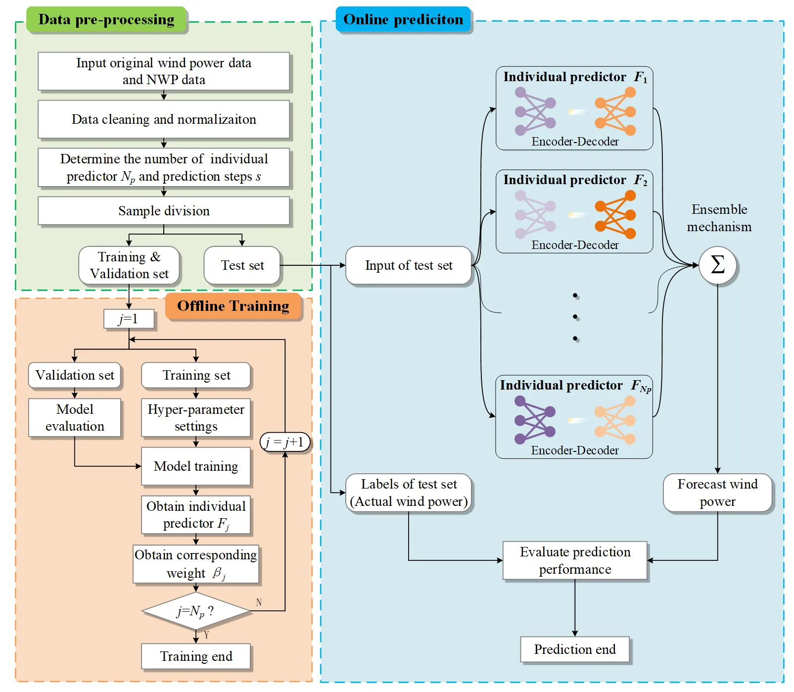
The procedure of using the proposed model for multi-step wind power prediction is displayed in
, including data pre-processing, offline training, and online prediction. The specific steps will be introduced below.
. Flowchart of the proposed model for multi-step wind power prediction.
In the data pre-process stage, the actual data for the forecast is preprocessed and then normalized. The normalization method is introduced in the case study. Next, we determine the number of individual predictors and prediction steps.
In the offline training stage, first, according to historical information length
p, future information length
q, and prediction step
s, historical data and NWP data will be divided to obtain training samples. The input of each sample includes the historical information input matrix
Xin,t and the future information input matrix
Win,t. The label is the wind power sequence $$\hat{\bm{y}}$$ corresponding to the prediction period. Next, all training samples are divided into three sets used for training, validation and test respectively. In the training model process, the hyper-parameters in the network are determined by the space search method. The model is evaluated by the validation set during the training process. Various parts of the training set can be used to build different predictors with distinct parameters.
In the online prediction stage, the test set is sequentially inputted into these trained predictors to obtain the forecast wind power sequence. The final result is the ensemble values of the outputs from these predictors. The actual value can be compared with the forecast value to evaluate the accuracy of the proposed prediction method.
5. Case Study and Analysis
5.1. Description and Pre-Process of the Wind Power Dataset
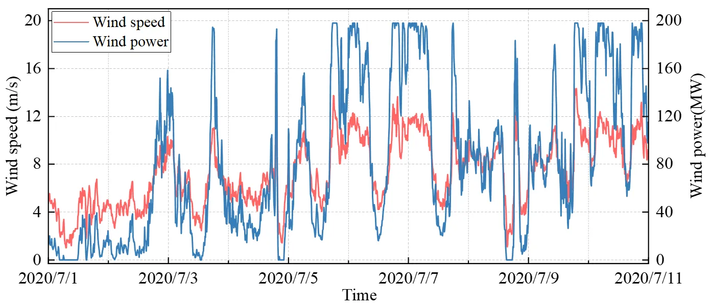
We use real wind farm data to verify the performance of the proposed prediction model. The real wind farm consists of 36 wind units, each with a capacity of 5.5 MW, for a total capacity of 198 MW. The dataset contains historical data, and the NWP data is given in Section 3.1. Data from July 2020 to September 2021 were collected for the forecast. The time step of historical information is 10 min, while the NWP in this wind farm has a 1-h interval within a 4-h prediction range, which is similar to a previous study [
35]. The curves of the wind speed and wind power from 1 July 2020, to 10 July 2020, are displayed in
. Wind power generation is closely related to the wind speed condition. Because of the uncertainty in wind speed changes, wind power exhibits obvious fluctuations, randomness, and an intermittent nature. Moreover, we use a public dataset from China Longyuan Power Group with 15 min temporal resolution to further verify the universality of the proposed prediction model, and the specific introduction is provided in Appendix A.
In accordance with the sample division method in Section 4.2, the existing data can be used to construct the research into a supervised learning problem. The original data are divided into two sets in a ratio of 9:1, which are used for training and test, respectively, and 10% of the training set is considered to be the validation set during training. This framework is completed in Python 3.6, and the forecast model is built under Pytorch and Scikit-learn. All the simulations were conducted on a computer equipped with an i9-10900 CPU and Nvidia P1000 GPU.
Because the values of wind power and weather features differed considerably, normalization is required in all input data to avoid the negative effect of value differences and ensure the training process remains stable. All data are scaled to a value between 0 and 1 through the min-max normalization method. After obtaining the normalized predicted value, the inverse normalization method can be used to obtain the real value. The min–max normalization can be expressed as follows:
where
x and
x∗ denote the real and normalized features, such as wind power, wind speed, and air pressure. Here,
xmin and
xmax represent the lower and upper limits of the feature, respectively.
. Wind speed and wind power curves.
The comparison between the proposed model and other prediction models, such as Bi-GRU & Bi-GRU, GRU–CNN, adaptive boosting regression (AdaBoost), and MSVR was conducted. The Bi-GRU & Bi-GRU model is set as the baseline model. Except for the data quality, the hyper-parameters of the model greatly affect forecast performance. Therefore, it is necessary to adjust the model hyper-parameters to determine a better combination of candidate hyper-parameters. Because of the large space for hyper-parameter optimization, manual experience and the grid search method were used simultaneously to define the hyper-parameters of the model in this study. First, a heuristic approach is adopted to determine the search interval of each hyperparameter. Then, the grid search method was applied to find the combination of hyper-parameters.
The key hyper-parameters of the proposed model included the number of hidden layers in the encoder (
lel,
le2) and the number of neurons in each layer (
ne1,
ne2). For convenience, the key-value pair vector dimensions of the two types of the MHA mechanism in the decoder were both set to
dm, the number of stacked decoding layers was
lm and the number of the head was set to eight. The Bi-GRU & Bi-GRU is a Seq2Seq model in which both encoder and decoder are composed of Bi-GRU. The GRU–CNN is a normal hybrid model that is used to predict wind power. Because of its excellent performance, the CNN was used in this hybrid model to process information obtained after the GRU layer processing. In addition to the hyper-parameters in the GRU module (
lgru,
ngru), the number of layers and the shape of the convolution kernel in the CNN module contribute considerably to the performance of this hybrid model. We used the convolutional kernel with a shape of 3 × 3 and max pooling to form a convolutional layer. The AdaBoost is a machine learning model based on the tree model and ensemble learning, and the number of integration estimators
nAdaBoost is a key factor. The performance of the MSVR is greatly influenced by the penalty coefficient
C and the kernel function type
kernel. In particular, AdaBoost and MSVR cannot receive multi-variable time-series input, so the input matrix should be expanded into a one-dimensional vector when applying these models. The search interval and selection of hyper-parameters in forecast models are listed in
.
.
Search interval and setting of hyper-parameters in forecast models.
| Forecast Model |
Search Interval |
Setting of Hyper-Parameters |
| Bi-GRU & Bi-GRU |
lel, le2, lm ∈ {1, 2, 3}
nel, ne2, dm ∈ {64, 96, 128, …, 256}
|
lel, le2 = 1, lm = 2
nel, ne2 = 128, dm = 128
|
| Proposed |
lel, le2, lm ∈ {1, 2, 3}
nel, ne2, dm ∈ {64, 96, 128, …, 256}
|
lel, le2 = 1, lm = 2
nel, ne2 = 128, dm = 256
|
| GRU–CNN |
lgru, lcnn ∈ {1, 2, 3}
ngru ∈ {64, 96, 128, …, 256}
|
lgru, lcnn = 2
ngru = 128
|
| AdaBoost |
nAdaBoost ∈ {5, 10, 15,…, 200} |
nAdaBoost = 10 |
| MSVR |
C ∈ {0.1, 1, 10, 100, 1000}
kernel ∈ {‘rbf’, ‘linear’, ‘sigmoid’}
|
C = 1
kernel = ‘rbf’
|
5.3. Evaluation Metrics
To evaluate the effect and accuracy of different prediction models, three evaluation metrics—namely, root mean square error (RMSE), mean absolute error (MAE) [
7], coefficient of determination (
R2), and Pearson correlation coefficient (PCC)—were considered. These metrics are defined as follows:
where $$y_{i}$$ and $$\hat{y}_{i}$$ represent the actual value and forecast value of wind power at period
i, respectively, $$\overset{-}{y}$$ and $$\overset{-}{\hat{y}}$$ denote the average value of actual and forecast output, respectively. Here,
n is the total number of time steps within this interval, and
CN is the rated capacity of the wind farm.
In addition, in order to describe the different error distributions, the two commonly used statistics are skewness and kurtosis, which are defined in (29) and (30), respectively. Skewness (
γ) is used to measure the asymmetry between the mean of the sample, and the smaller the absolute value, the more symmetrical the distribution, and the higher the reliability. If the skewness of the model is greater than 0, it is positive skewness, and the distribution is right-biased, that is, the right tail of the data is longer.
where
γ represents the skewness value, which represents the asymmetry of the distribution. $$E \left( x - \mu \right)^{3}$$ represents the third-power expected value of the difference between the data point and the mean, reflecting the degree of asymmetry in the distribution of the data.
μ is the mean of the sample, which represents the central position of the data distribution. $$\sigma$$ is the standard deviation of the sample, which indicates the degree of discreteness of the data distribution.
Kurtosis (
β) measures the sharpness of the data distribution, and smaller kurtosis indicates a flatter data distribution, fewer extremes, thinner tails, and higher reliability. That is
5.4. Forecast Results and Analysis
To evaluate the performance of forecast models, the wind power for 1, 2, 3, and 4 h in the future (6, 12, 18, and 24 steps, respectively) were predicted.
lists the prediction errors of all models and the time for model training, verification, and testing. We analyze the results from the evaluation indicators and time.
The RMSE of the proposed model in four prediction scenarios is 2.57%, 3.56%, 4.54% and 5.38%, respectively, and the MAE is 2.08%, 2.85%, 3.63% and 4.30%, respectively. Among these models, the proposed model has the lowest RMSE and MAE, and prediction accuracy of more than 94%. Specifically, the RMSE of the proposed model is reduced by 25.99~36.70% compared with Bi-GRU & Bi-GRU, indicating that MHA could capture the diverse information in the sequence more comprehensively than Bi-GRU in the decoder. It is 22.5~49% lower than that of GRU-CNN, which indicates that the Bi-GRU and MHA had a stronger ability to extract critical information in time series than those of the GRU and CNN. It is 16.7~59% lower than that of AdaBoost and MSVR, which indicates that the proposed model outperforms other forecast models without the encoder–decoder architecture, which also proves that the encoder–decoder architecture is more suitable for S2S prediction tasks. However, its
R2 is the largest, indicating that it can perform best in the ultra-short-term forecast of wind power. From the perspective of prediction scenarios, the prediction error of each model increases with the increase in the prediction time. Thus, the superiority of the proposed model can be effectively verified.
The training time of these models is longer than that of the non-cross-validation model due to the use of 5-fold time series cross-validation. Obviously, the more the fold, the longer the training time, but the accuracy can be significantly improved, but combined with
, it can be found that the accuracy performance is significantly improved. With the increase of prediction time steps, the training time of Bi-GRU & Bi-GRU, GRU-CNN and the proposed model becomes shorter. Taking the proposed model as an example, the average running time of each iteration in the training, that is, the running speed of each iteration, can reflect the efficiency of model training: 0.5089 s/iter at 4 h; 0.4863 s/iter at 3 h; 0.2589 s/iter at 2 h; At 1 h, it is 0.2147 s/iter. It can be found that the longer the prediction time steps, the faster the average running speed of each iteration. This explains why the training time is inversely proportional to with the prediction time steps. The specific reasons are that the wind farm involves a large amount of data. When loading data in the encoder-decoder structure for a longer prediction sequence, it avoids the overhead of multiple loading and data migration though the sample size processed in a single instance becomes large. Additionally, longer prediction sequences converge faster in deep learning timing neural networks, so that the model can reach the minimum validation loss quickly, thus triggering the early stop mechanism.
The AdaBoost and MSVR belong to ensemble learning and support vector machines, which are different from the neural network structures in deep learning such as GRU-CNN, the proposed model, and Bi-GRU & Bi-GRU, so the way of realizing power prediction is also different. Its training time increases with the increase of prediction time steps, which aligns with the trend of normal cross-validation.
Compared with Bi-GRU & Bi-GRU, the training time required for the proposed model is shorter at all forecasting scenarios, whereas the training time required for the proposed model is shorter than that of the GRU-CNN at 1h and 4h, and the time difference between 2 h and 3 h is not much difference compared with the GRU-CNN. The training time of the proposed model is not as good as that of the AdaBoost and MSVR with non-encoder-decoder structure, indicating that the deep learning timing neural network requires more training time, but the corresponding accuracy can be improved by more than 16.7%, making up for the cost of time. In addition, we observed negligible test times for all models.
To further evaluate the prediction ability of all the models on the test set, the forecast values of the test set were divided into subsets to calculate the RMSE and MAE of one prediction processing. For the 2-h prediction scenario, approximately 961 subsets were considered, and the number of values in one subset was 12, the RMSE and MAE of all subsets can be computed according to
Equation (25) and
Equation (26) (
n = 12).
shows the RMSE distribution under the 2-h and 4-h prediction scenarios of different models.
lists the distribution of MAE under 2-h and 4-h prediction scenarios for different models. Taking 2-h as an example, the upper quartiles of RMSE and MAE were 4.38 and 3.66, respectively, which indicated that the RMSE and MAE of more than 75% of test samples from the proposed model were within 4.38% and 3.66%. The error distributions of the proposed model were considerably better than those of other models. We also calculated the RMSEs and MAEs of the subsets in the 4-h prediction scenarios. Approximately 481 subsets existed, the results are similar to that under 2-h and 4-h prediction scenarios. Obviously, the upper and lower quartiles, mean, and median of the proposed model are the smallest among the models, which means that the overall performance of the proposed model in the two prediction scenarios is the best among all models.
In order to analyze the distribution of prediction errors of each model in more detail and judge the reliability of the model,
also shows the skewness and kurtosis under the 2-h and 4-h prediction scenarios of different models. The skewness and kurtosis can be computed according to
Equation (29) and
Equation (30).
shows that the skewness of the four models is greater than 0, which is positive skewness, and the kurtosis is greater than 1, indicating that the error data has a certain skewness and is not normally distributed. Therefore, our interpretation of kurtosis needs to be considered in conjunction with skewness. The skewness of the proposed model is the smallest among the four models under the prediction scenarios of 2-h and 4-h. It reaches a minimum value of 1.60 at 4-h, indicating that the error distribution of the proposed method is the most symmetrical, and the extreme value (outlier) has the least influence on the mean and median. Similar to skewness, the kurtosis of the proposed model is the smallest among the four models under the two prediction scenarios, indicating that the error distribution of the proposed method has the smallest deviation among the four models, the sudden peak change is smaller, and the tail characteristics are the most similar to the normal distribution. Therefore, due to the asymmetry of the error distribution and a certain skewness, we comprehensively consider the skewness and kurtosis, and conclude that the proposed model has less skewness and kurtosis and is more reliable in most prediction scenarios.
.
Comparison of prediction error and runtime of all models under different forecasting scenarios.
| Prediction Scenarios |
Model |
RMSE(%) |
MAE(%) |
R2 |
Train-Time |
Test-Time |
| 1 h (6 steps) |
Bi-GRU & Bi-GRU |
4.06 |
2.84 |
0.9346 |
5716.39 s |
0.01 s |
| Proposed |
2.57 |
2.08 |
0.9470 |
4740.26 s |
0.01 s |
| GRU–CNN |
5.03 |
4.25 |
0.9177 |
6533.37 s |
0.01 s |
| AdaBoost |
6.27 |
5.02 |
0.8763 |
1420.97 s |
0.01 s |
| MSVR |
6.13 |
4.90 |
0.8892 |
1023.48 s |
0.00 s |
| 2 h (12 steps) |
Bi-GRU & Bi-GRU |
4.97 |
3.98 |
0.9187 |
4866.03 s |
0.01 s |
| Proposed |
3.56 |
2.85 |
0.9365 |
4008.32 s |
0.00 s |
| GRU–CNN |
5.07 |
4.06 |
0.9164 |
3994.19 s |
0.00 s |
| AdaBoost |
6.37 |
5.10 |
0.8842 |
1934.35 s |
0.00 s |
| MSVR |
7.39 |
5.91 |
0.8414 |
1269.21 s |
0.00 s |
| 3 h (18 steps) |
Bi-GRU & Bi-GRU |
6.42 |
5.14 |
0.8829 |
4132.69 s |
0.01 s |
| Proposed |
4.54 |
3.63 |
0.9240 |
2614.91 s |
0.00 s |
| GRU–CNN |
5.99 |
4.79 |
0.9063 |
2560.72 s |
0.00 s |
| AdaBoost |
6.74 |
5.39 |
0.8761 |
2436.28 s |
0.00 s |
| MSVR |
8.15 |
6.52 |
0.8286 |
1963.54 s |
0.00 s |
| 4 h (24 steps) |
Bi-GRU & Bi-GRU |
7.27 |
5.82 |
0.8469 |
3590.24 s |
0.00 s |
| Proposed |
5.38 |
4.30 |
0.9105 |
1567.51 s |
0.01 s |
| GRU–CNN |
6.94 |
5.55 |
0.8749 |
2302.37 s |
0.01 s |
| AdaBoost |
6.46 |
5.17 |
0.8814 |
2989.96 s |
0.00 s |
| MSVR |
8.29 |
6.63 |
0.8257 |
2176.49 s |
0.00 s |
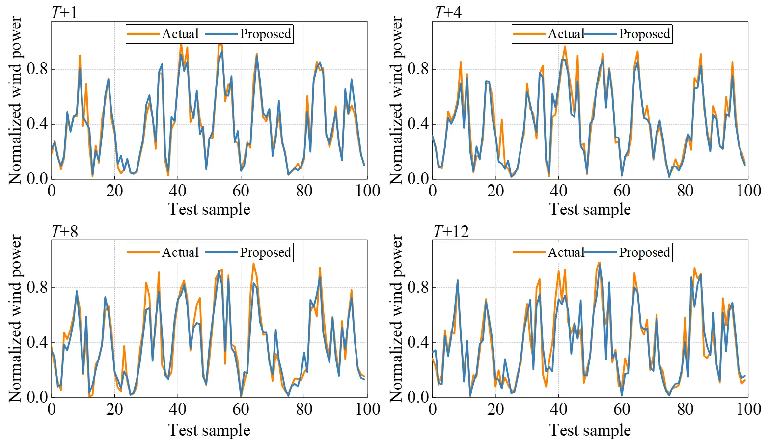
To analyze the forecast results in detail, we discussed the error of the proposed model at each prediction time step. Considering 2-h prediction (12 steps) as an example, approximately 961 test samples were obtained, and the output of each test sample was a forecast wind power sequence of length 12. Subsequently, the forecast results could be formed into a matrix $$\bm{Y}_{t e s t} \in R^{961 \times 12}$$. The first column of this matrix represented the forecast result in the first step (
T + 1), and the last column represented the forecast result in the twelfth step (
T + 12).
displays the actual and forecast wind power of 100 test samples at time step
T + 1,
T + 4,
T + 8, and
T + 12. It can be observed that the gap between the real curve and the prediction curve is small. The evaluation indicators of the forecast result at each time step calculated by
Equation (25),
Equation (26),
Equation (27) and
Equation (28) (
n = 961) are listed in
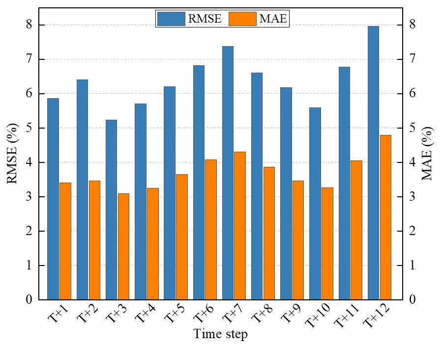
. The range of the RMSE calculated according to the time step was 5.24% to 7.96%. Even in the farthest time step from the observed time,
T + 12, the RMSE was still lower than 8%, which could help wind farms satisfy the more severe assessment indicators.
shows a bar chart corresponding to
, which helps readers intuitively observe the error change at each time step.
reveals that the forecast results of the proposed model did not exhibit obvious cumulative error, which indicates that the prediction error at a subsequent time step was not necessarily larger than that at an earlier time step. The result indicated the advantage of the generative method in the decoder compared with the recursive manner.
.
Distribution of RMSE (%) and skewness and kurtosis for different forecast models.
| Prediction Scenarios |
Forecast Model |
Mean |
Lower Quartile |
Median |
Upper Quartile |
Skewness |
Kurtosis |
2 h
(12 steps)
|
Bi-GRU & Bi-GRU |
4.97 |
1.81 |
3.54 |
6.01 |
3.00 |
13.59 |
| Proposed |
3.56 |
1.29 |
2.43 |
4.38 |
2.80 |
10.95 |
| GRU–CNN |
5.07 |
1.88 |
3.29 |
6.68 |
2.87 |
10.68 |
| AdaBoost |
6.37 |
4.31 |
5.06 |
7.91 |
3.27 |
21.43 |
| MSVR |
7.39 |
4.73 |
5.19 |
9.37 |
3.05 |
13.13 |
4 h
(24 steps)
|
Bi-GRU & Bi-GRU |
7.27 |
3.65 |
5.46 |
9.20 |
1.88 |
3.74 |
| Proposed |
5.38 |
1.87 |
3.92 |
7.11 |
1.60 |
2.60 |
| GRU–CNN |
6.94 |
3.97 |
5.85 |
8.12 |
2.61 |
8.18 |
| AdaBoost |
6.46 |
3.82 |
5.38 |
7.47 |
2.84 |
13.59 |
| MSVR |
8.29 |
4.45 |
7.97 |
11.52 |
1.89 |
3.97 |
.
Distribution of MAE (%) for different forecast models.
| Prediction Scenarios |
Forecast Model |
Mean |
Lower Quartile |
Median |
Upper Quartile |
| 2 h (12 steps) |
Bi-GRU & Bi-GRU |
3.98 |
1.20 |
2.77 |
4.88 |
| Proposed |
2.85 |
1.01 |
2.06 |
3.66 |
| GRU–CNN |
4.06 |
1.65 |
2.74 |
5.31 |
| AdaBoost |
5.10 |
3.66 |
4.08 |
6.54 |
| MSVR |
5.91 |
3.85 |
4.12 |
7.46 |
| 4 h (24 steps) |
Bi-GRU & Bi-GRU |
5.82 |
3.28 |
4.44 |
7.31 |
| Proposed |
4.30 |
1.69 |
3.23 |
5.76 |
| GRU–CNN |
5.55 |
3.24 |
4.78 |
6.53 |
| AdaBoost |
5.17 |
3.06 |
4.30 |
5.98 |
| MSVR |
6.63 |
3.62 |
6.38 |
9.47 |
. Forecast results at <i>T</i> + 1, <i>T</i> + 4, <i>T</i> + 8, and <i>T</i> + 12 in the 2-h prediction scenario.
. Bar chart of the error at each time step of the proposed model.
.
Evaluation at each time step of the proposed model.
| Time Step |
RMSE (%) |
MAE (%) |
R2 |
PCC |
| T + 1 |
5.86 |
3.41 |
0.9311 |
0.9650 |
| T + 2 |
6.40 |
3.46 |
0.9158 |
0.9574 |
| T + 3 |
5.24 |
3.09 |
0.9467 |
0.9733 |
| T + 4 |
5.70 |
3.25 |
0.9381 |
0.9696 |
| T + 5 |
6.21 |
3.64 |
0.9247 |
0.9621 |
| T + 6 |
6.82 |
4.08 |
0.9073 |
0.9528 |
| T + 7 |
7.37 |
4.31 |
0.8963 |
0.9478 |
| T + 8 |
6.60 |
3.86 |
0.9110 |
0.9545 |
| T + 9 |
6.18 |
3.46 |
0.9250 |
0.9623 |
| T + 10 |
5.59 |
3.26 |
0.9368 |
0.9680 |
| T + 11 |
6.77 |
4.05 |
0.9129 |
0.9560 |
| T + 12 |
7.96 |
4.79 |
0.8805 |
0.9385 |
6. Conclusions
To address the intermittent and fluctuating nature of wind power for the safe and economic operation of the power grid, this study proposed a novel encoder–decoder based hybrid model for wind power multi-step prediction. Bi-GRU, MHA, and ensemble technique were combined in the model. Comparative simulations using actual data were conducted to validate the proposed model. Conclusions from this paper are as follows:
- 1.
-
The proposed model outperformed other existing models in four prediction scenarios (1-, 2-, 3-, and 4-h prediction). The RMSEs of predicted outputs from the proposed model in four prediction scenarios were 2.57%, 3.56%, 4.54% and 5.38%, which were 25.99~36.70%, 22.5~49%, 16.7~59% and 35.1~53.7%, respectively, lower than those from other forecast models, respectively. The MAEs of results from the proposed model in four prediction scenarios were 2.08%, 2.85%, 3.63% and 4.30%, which were 26.13~29.38%, 22.52~51.06%, 16.44~58.37% and 35.13~57.55%,respectively, lower than those from other forecast models. In terms of the wind power curve fitting, the R2 of predicted outputs from the proposed model were higher than 0.91, respectively. This means that the MHA has a stronger ability to extract information in time series, and the prediction framework based on the encoder–decoder architecture is more suitable for S2S prediction tasks, such as wind power multi-step prediction.
- 2.
-
The training time of the proposed model is the shortest under the four prediction scenarios of deep learning neural network structure, with a training time of 1567.51 s and a test time of 0.01 s in the 4 h prediction scenario, and hence it is suitable for deployment in real-time energy systems.
- 3.
-
The proposed model can be used to perform reliable prediction. The RMSE of more than 75% of test samples from the proposed model were within 4.38% in the 2-h prediction scenario, and the error distributions of the proposed model were considerably better than those of other models.
- 4.
-
The proposed model did not exhibit obvious cumulative error in the multi-step prediction. From the error change at each time step, the prediction error at a subsequent time step was not necessarily larger than that at an earlier time step.
Appendix A
In Section 5, the wind power dataset is from an offshore wind farm in eastern China. In Appendix A, we have supplemented a new public wind data set covering the period from 2 October 2021 to 16 November 2022 (hereinafter referred to as the public dataset), with historical information and NWP data using a 15-min time resolution—from the 2023 New Energy Intelligent Algorithm Competition hosted by China Longyuan Power Group (
https://aistudio.baidu.com/ datasetdetail/212945, accessed on 15 July 2025), to validate the model we propose. This inclusion helps demonstrate the model’s suitability for different geographic locations, with details listed in Table A1.
Table A1.
Error statistics of all models under different prediction scenarios.
| Prediction Scenarios |
Model |
RMSE (%) |
MAE (%) |
R2 |
| 1 h (4 steps) |
Proposed |
4.72 |
3.78 |
0.9277 |
| GRU–CNN |
5.19 |
4.15 |
0.9137 |
| AdaBoost |
8.42 |
6.74 |
0.8193 |
| MSVR |
6.47 |
5.18 |
0.8810 |
| 2 h (8 steps) |
Proposed |
6.79 |
5.43 |
0.8752 |
| GRU–CNN |
7.05 |
5.64 |
0.8612 |
| AdaBoost |
10.42 |
8.34 |
0.7992 |
| MSVR |
8.78 |
7.02 |
0.8146 |
| 3 h (12 steps) |
Proposed |
7.99 |
6.39 |
0.8351 |
| GRU–CNN |
8.66 |
6.93 |
0.8153 |
| AdaBoost |
10.48 |
8.38 |
0.7981 |
| MSVR |
9.82 |
7.86 |
0.8079 |
| 4 h (16 steps) |
Proposed |
9.53 |
7.62 |
0.8095 |
| GRU–CNN |
10.03 |
8.02 |
0.8016 |
| AdaBoost |
11.63 |
9.30 |
0.7898 |
| MSVR |
10.97 |
8.78 |
0.7969 |
As can be seen from Table A1, the proposed model has the lowest RMSE and MAE in all prediction scenarios, indicating that the prediction error is the smallest, and the prediction accuracy is the highest, with an accuracy of more than 90%. Specifically, the RMSE of the proposed model is 3.69~4.99% lower than that of GRU-CNN, 18.06~43.94% lower than that of AdaBoost, and 13.13~27.05% lower than that of MSVR. But the
R2 of the proposed model is the largest, which shows that it has the best fitting effect. Thus, we can verify that the proposed model has superiority and generalizability in different regions.
Acknowledgments
We thank LetPub (www.letpub.com.cn) for its linguistic assistance during the preparation of this manuscript.
Author Contributions
Conceptualization, S.Z.; Methodology, S.Z. and M.L.; Software, S.Z.; Validation, Y.L. and Q.H.; Formal Analysis, S.Z.; Investigation, Y.L. and Q.H.; Resources, Y.L. and Q.H.; Data Curation, Y.L. and Q.H.; Writing—Original Draft Preparation, S.Z.; Writing—Review & Editing, M.L.; Visualization, Y.L. and Q.H.; Supervision, M.L.; Project Administration, M.L.; Funding Acquisition, M.L
Ethics Statement
Not applicable.
Informed Consent Statement
Not applicable.
Data Availability Statement
Not applicable.
Funding
This research was funded by Guangdong Basic and Applied Basic Research Foundation (Grant number: 2024B1515250007).
Declaration of Competing Interest
The authors declare that they have no known competing financial interests or personal relationships that could have appeared to influence the work reported in this paper.
References
-
1.
Farah S, David AW, Humaira N, Aneela Z, Steffen E. Short-term multi-hour ahead country-wide wind power prediction for Germany using gated recurrent unit deep learning.
Renew. Sustain. Energy Rev. 2022,
167, 112700.
[Google Scholar]
-
2.
Global Wind Report 2025. Global Wind Energy Council (GWEC). 2025. Available online: https://www.gwec.net/reports/globalwind report (accessed on 20 May 2025).
-
3.
Wang H, Lei Z, Zhang X, Zhou B, Peng J. A review of deep learning for renewable energy forecasting.
Energy Convers. Manag. 2019,
198, 111799.
[Google Scholar]
-
4.
Xue H, Jia Y, Wen P, Farkoush SG. Using of improved models of Gaussian processes in order to regional wind power forecasting.
J. Clean. Prod. 2020,
262, 121391.
[Google Scholar]
-
5.
Tawn R, Browell J. A review of very short-term wind and solar power forecasting.
Renew. Sustain. Energy Rev. 2022,
153, 111758.
[Google Scholar]
-
6.
Wan C, Xu Z, Wang Y, Dong ZY, Wong KP. A hybrid approach for probabilistic forecasting of electricity price.
IEEE Trans. Smart Grid 2014,
5, 463–470.
[Google Scholar]
-
7.
Prieto-Herraez D, Martinez-Lastras S, Frias-Paredes L, Asensio MI, Gonzalez-Aguilera D. EOLO, a wind energy forecaster based on public information and automatic learning for the Spanish Electricity Markets.
Measurement 2024,
231, 114557.
[Google Scholar]
-
8.
Wang Y, Zou R, Liu F, Zhang L, Liu Q. A review of wind speed and wind power forecasting with deep neural networks.
Appl. Energy 2021,
304, 117766.
[Google Scholar]
-
9.
Chen C, Liu H. Dynamic ensemble wind speed prediction model based on hybrid deep reinforcement learning.
Adv. Eng. Inform. 2021,
48, 101290.
[Google Scholar]
-
10.
Afrasiabi M, Mohammadi M, Rastegar M, Afrasiabi M. Advanced deep learning approach for probabilistic wind speed forecasting.
IEEE Trans. Ind. Inform. 2021,
17, 720–727.
[Google Scholar]
-
11.
Hong YY, Rioflorido CLPP. A hybrid deep learning-based neural network for 24-h ahead wind power forecasting.
Appl. Energy 2019,
250, 530–539.
[Google Scholar]
-
12.
Wang H, Lei Z, Liu Y, Peng J, Liu J. Echo state network based ensemble approach for wind power forecasting.
Energy Convers. Manag. 2019,
201, 112188.
[Google Scholar]
-
13.
Liu MD, Ding L, Bai YL. Application of hybrid model based on empirical mode decomposition, novel recurrent neural networks and the ARIMA to wind speed prediction.
Energy Convers. Manag. 2021,
233, 113917.
[Google Scholar]
-
14.
Tian Z. Short-term wind speed prediction based on LMD and improved FA optimized combined kernel function LSSVM.
Eng. Appl. Artif. Intell. 2020,
91, 103573.
[Google Scholar]
-
15.
Qu Z, Zhang K, Mao W, Wang J, Liu C, Zhang W. Research and application of ensemble forecasting based on a novel multi-objective optimization algorithm for wind-speed forecasting.
Energy Convers. Manag. 2017,
154, 440–454.
[Google Scholar]
-
16.
Chen J, Zeng GQ, Zhou W, Du W, Lu K-D. Wind speed forecasting using nonlinear-learning ensemble of deep learning time series prediction and extremal optimization.
Energy Convers. Manag. 2018,
165, 681–695.
[Google Scholar]
-
17.
Wang J, Hu J, Ma K, Zhang Y. A self-adaptive hybrid approach for wind speed forecasting.
Renew. Energy 2015,
78, 374–385.
[Google Scholar]
-
18.
Lu P, Ye L, Zhao Y, Dai B, Pei M, Li Z. Feature extraction of meteorological factors for wind power prediction based on variable weight combined method.
Renew. Energy 2021,
179, 1925–1939.
[Google Scholar]
-
19.
Xiao L, Qian F, Shao W. Multi-step wind speed forecasting based on a hybrid forecasting architecture and an improved bat algorithm.
Energy Convers. Manag. 2017,
143, 410–430.
[Google Scholar]
-
20.
Tian Z, Chen H. Multi-step short-term wind speed prediction based on integrated multi-model fusion.
Appl. Energy 2021,
298, 117248.
[Google Scholar]
-
21.
Wang J, Song Y, Liu F, Hou R. Analysis and application of forecasting models in wind power integration: A review of multi-step-ahead wind speed forecasting models.
Renew. Sustain. Energy Rev. 2016,
60, 960–981.
[Google Scholar]
-
22.
Bontempi G, Ben Taieb S, Le Borgne YA. Machine learning strategies for time series forecasting. In Business Intelligence; Aufaure MA, Zimanyi E, Eds.; Springer-Verlag: Berlin, Germany, 2013; Volume 138, pp. 62–77.
-
23.
Ben Taieb S, Sorjamaa A, Bontempi G. Multiple-output modeling for multi-step-ahead time series forecasting.
Neurocomputing 2010,
73, 1950–1957.
[Google Scholar]
-
24.
Niu Z, Yu Z, Tang W, Wu Q, Reformat M. Wind power forecasting using attention-based gated recurrent unit network.
Energy 2020,
196, 117081.
[Google Scholar]
-
25.
Fan C, Wang J, Gang W, Li S. Assessment of deep recurrent neural network-based strategies for short-term building energy predictions.
Appl. Energy 2019,
236, 700–710.
[Google Scholar]
-
26.
Bao Y, Xiong T, Hu Z. Multi-step-ahead time series prediction using multiple-output support vector regression.
Neurocomputing 2014,
129, 482–493.
[Google Scholar]
-
27.
Lu K, Sun WX, Wang X, Meng XR, Zhai Y, Li HH, et al. Short-term wind power prediction model based on encoder-decoder LSTM. In Proceedings of the International Conference of Green Buildings and Environmental Management (GBEM 2018), Qingdao, China, 23–25 August 2018.
-
28.
Neshat M, Nezhad MM, Mirjalili S, Piras G, Garcia DA. Quaternion convolutional long short-term memory neural model with an adaptive decomposition method for wind speed forecasting: North aegean islands case studies.
Energy Convers. Manag. 2022,
259, 115590.
[Google Scholar]
-
29.
Wang L, He Y, Li L, Liu X, Zhao Y. A novel approach to ultra-short-term multi-step wind power predictions based on encoder–decoder architecture in natural language processing.
J. Clean. Prod. 2022,
354, 131723.
[Google Scholar]
-
30.
Vaswani A, Shazeer N, Parmar N, Uszkoreit J, Jones L, Gomez AN, et al. Attention is all you need. In Proceedings of the 31st Conference on Neural Information Processing Systems (NIPS 2017), Long Beach, CA, USA, 4–9 December 2017.
-
31.
Wang L, He Y, Liu X, Li L, Shao K. M2TNet: Multi-modal multi-task Transformer network for ultra-short-term wind power multi-step forecasting.
Energy Rep. 2022,
8, 7628–7642.
[Google Scholar]
-
32.
Zhou H, Zhang S, Peng J, Zhang S, Li J, Xiong H, et al. Informer: Beyond efficient Transformer for long sequence time-series forecasting. In Proceedings of the Thirty-fifth AAAI Conference on Artificial Intelligence, Virtual Conference, 2–9 February 2021.
-
33.
Yang T, Yang Z, Li F, Wang H. A short-term wind power forecasting method based on multivariate signal decomposition and variable selection.
Appl. Energy 2024,
360, 122759.
[Google Scholar]
-
34.
Chung J, Gulcehre C, Cho K, Bengio Y. Empirical evaluation of gated recurrent neural networks on sequence modeling.
arXiv 2014, arXiv:1412.3555.
[Google Scholar]
-
35.
Wang H, Zhang YM, Mao JX. Sparse Gaussian process regression for multi-step ahead forecasting of wind gusts combining numerical weather predictions and on-site measurements.
J. Wind. Eng. Ind. Aerodyn. 2022,
220, 104873.
[Google Scholar]