Rolling Bearing Health Indicator: From Design to Modeling
and Evaluation

Huang, Gangjin; Wu, Shanshan; Wang, Quan; Wei, Wuguo; Fu, Yaoming; Wang, Nan; Lei, Lijie

doi:10.70322/ism.2025.10025

lssue 2, Volume 2

Article Open Access

Rolling Bearing Health Indicator: From Design to Modeling and Evaluation

Gangjin Huang ¹ Shanshan Wu ² Quan Wang ¹ Wuguo Wei ¹ Yaoming Fu ¹ Nan Wang ^1,* Lijie Lei ¹

Author Information

Other Information

Aviation Engineering Institute, Civil Aviation Flight University of China, Chengdu 641450, China

School of Information Engineering, Sichuan Agricultural University, Ya’an 625000, China

Authors to whom correspondence should be addressed.

Received: 18 June 2025 Accepted: 05 August 2025 Published: 08 August 2025

Downloads:3

Intell. Sustain. Manuf. 2025, 2(2), 10025; DOI: 10.70322/ism.2025.10025

ABSTRACT: As a key component of industrial machinery, accurate prediction of the degradation trend of rolling bearings is crucial for equipment safety. However, traditional health indicator (HI) extraction methods often suffer from feature redundancy, and prediction models lack the ability to capture spatial dimension features, leading to significant prediction errors. To address these issues, 16 time-frequency domain features were first extracted, and a new HI was constructed by combining the Gaussian Process latent variable model (GPLVM) for non-linear feature fusion and exponentially weighted moving average (EWMA) for smoothing. Additionally, a spatial-temporal convolutional long short-term memory network (ST-CNet) was proposed, which integrates a 3-layer CLSTM, fully connected layers, and batch normalization to effectively capture local and long-term spatiotemporal dependencies. Case studies on IMS bearing datasets show that the constructed HI accurately describes the degradation process, and ST-CNet achieves superior performance with lower MAE and RMSE compared to existing methods.

Keywords: Prediction of degradation trend; Multi-feature fusion; ST-CNet; Rolling bearing; Health indicator

1. Introduction

Rolling bearings are widely used in various industrial equipment as a core component of rotating machinery. However, during the operation of the equipment, due to the complex operating environment and the influence of various unfavorable factors, rolling bearings will gradually wear out until failure. The rolling bearing degradation process not only affects the daily operation of the whole working system, but also may cause serious accidents, resulting in casualties and significant economic losses. Therefore, it is significant to study the rolling bearing degradation trend prediction technology [1,2,3]. There are two core steps in rolling bearing degradation trend prediction. Firstly, how to construct a suitable health index to reflect the degradation state of rolling bearings. Secondly, to construct a suitable prediction model to predict the degradation trend of rolling bearings. Currently, in the research on health index, Yan et al. [4] proposed a novel health index based on sparse representation to describe the degradation trend. Chen et al. [5] proposed improved Gini indices to quantify the transient impulse features of rolling bearings. Considering the influence of all spectral amplitudes in the frequency domain on the degradation degree of mechanical equipment, Yan et al. [6] proposed a health indicator based on Fisher’s discrimination ratio. However, it is difficult for a single feature to fully reflect the degradation process of the rolling bearings. Gu et al. [7] utilized evaluation indexes to select the sensitive indicators, after which the degradation indicators were fused through isometric feature mapping. Chen et al. [8] extracted multi-domain high-dimensional features and constructed a health indicator based on a deep convolutional auto-encoder. However, extracting multiple features without choosing a suitable feature fusion method can lead to feature redundancy in the extracted health indicators and the existence of partial fluctuations in the health index, which affects the prediction accuracy of the network model. The degradation and failure of rolling bearings are mainly caused by rolling contact fatigue, which results from the cumulative cyclic stress in the contact area between rolling elements and raceways [9,10]. Their fatigue life is closely related to boundary zone properties, especially the residual stress state beneath the surface [11,12]. Manufacturing processes like hard turning and deep rolling can induce a depth-dependent residual stress state [13,14], and high compressive residual stresses within 300 μm below the surface can significantly delay the initiation and propagation of fatigue cracks [15,16]. Recent research by Wu et al. [17] explored the rolling contact fatigue (RCF) behavior of bearing steel under different surface roughness conditions. Their findings showed that surface roughness not only affects the stress distribution at the contact surface but also interacts with the residual stress state, influencing the fatigue crack initiation and propagation. Experiments have shown that such pre-induced residual stresses can increase the L10 bearing life by a factor of 2.5 [18,19], providing crucial mechanical background for understanding bearing degradation mechanisms and developing more practical health indicators and prediction models [20,21]. Secondly, in constructing the prediction model, the early methods are mainly based on experience and rules, such as life curves and empirical formulas, but their accuracy and applicability are limited. With the progress of science and technology, there are now two main methods for predicting the degradation trend of rolling bearings. One is the model-based method [22], which describes the bearing degradation process by establishing a mathematical or physical model. However, this method’s establishment and parameters estimation are complicated and have limited adaptability to complex and variable actual working conditions, resulting in low generalization ability and accuracy. The other is the data-driven approach [23], which includes regression-based models [24], methods based on stochastic processes [25], and the utilization of machine learning techniques[26], especially the widely used deep learning. Xia et al. [27] proposed a two-stage fault prediction method based on Deep Neural Networks (DNN) to predict the degradation trend through automatic feature extraction of data, which effectively solves the limitations of model-based methods. Cheng et al. [28] used deep convolutional neural networks (CNN) to automatically estimate and predict the degradation of bearings. Le et al. [29] used a back propagation neural network (BPNN) and a genetic algorithm to optimize the network parameters to achieve the prediction of rolling bearing degradation trend. Guo et al. [30] used Recursive Neural Network (RNN) health indicators to predict the bearing RUL. However, RNN suffers from the problems of gradient vanishing and gradient explosion, and improved RNN variants have been proposed, such as LSTM [31] and gate recurrent unit (GRU) [32], which alleviate the problems of gradient vanishing, explosion, and information forgetting, et al. by introducing a gate mechanism and a memory unit. Hu et al. [33] used LSTM combined with an improved particle swarm optimization algorithm to optimize the model parameters to accurately predict bearing degradation trends. Zheng et al. [34] based on the gated recirculation unit (GRU) prediction method for rolling bearing performance degradation based on Optimal wavelet packet and martensitic distances accurately predicted the bearing degradation trends, which helped the maintenance personnel to keep track of the health of their equipment. Huang et al. [35] used a bi-directional long and short-term memory neural network (Bi-LSTM) to model time series data, demonstrating its advantages and non-linear modeling ability in remaining life prediction of complex products, which can provide more accurate estimation results for remaining life prediction. Although GRU and LSTM perform well in handling sequential data and long-term dependencies, they are unable to fully utilize the spatial dimension of the features which is the distribution of vibration amplitudes at different time points. The ability to capture local features in spatio-temporal data is relatively weak. To solve the above problems, this paper proposes a rolling bearing degradation trend prediction method based on an improved multi-feature fusion health indicator and ST-CNet. On the one hand, the multi-domain features are simple to compute and can effectively characterize the bearing degradation state in practical engineering applications. GPLVM is utilized as a dimensionality reduction tool to filter the multi-domain features, and a HI is obtained to better depict the degradation trend of industrial machinery. EWMA is employed to further modify the HI, making it possible to improve the prediction ability. On the other hand, utilizing the spatiotemporal feature extraction capability of ST-CNet, a new prediction model was established for the deep prediction of the degradation trend of rolling bearings. Finally, the measured data verifies the feasibility of the proposed method. The remainder of this paper on the health indicator design is given in Section 2. The detailed framework of the proposed method is introduced in Section 3. In Section 4, a case study is applied to validate the effectiveness of the proposed method. At last, the conclusions are summarized. Notably, recent reviews have pointed out critical limitations in existing research [36,37]. He et al. emphasized that current health indicators often fail to balance non-linearity and monotonicity, with fusion methods like PCA struggling to capture complex degradation patterns in high-dimensional data [38,39]. As highlighted by Zhang et al. [40], the non—linear nature of bearing degradation requires more advanced feature extraction techniques that can adapt to the complex and changing operating conditions. Qiu et al. highlighted that data—driven models, despite advancements, still lack effective mechanisms to integrate spatial and temporal features [41,42]. For instance, CNN-based methods excel in spatial extraction but overlook temporal dependencies, while LSTM variants focus on time series but ignore local vibration characteristics [43]. Moreover, as discussed by Li et al., noise-induced fluctuations in health indicators remain a persistent issue, as conventional smoothing techniques lack adaptability to dynamic operating conditions. Addressing these gaps, this study proposes a novel framework combining multi-feature fusion and spatio-temporal modeling to enhance degradation trend prediction accuracy, with the specific methodology detailed in subsequent sections.

2. Health Indicator Design

This section focuses on constructing the health indicator (HI) to address issues of feature redundancy and fluctuations in traditional HIs, aiming to more accurately characterize the degradation process of rolling bearings through multi-domain feature extraction, non-linear fusion, and smoothing. 2.1. Time/Frequency Domain Feature Extraction Time-domain and frequency-domain features are the most widely used features in practical engineering applications, with the advantages of simple calculation and easy access at the edge end. From the point of view of physical mechanism, the time domain features (e.g., mean, peak, RMS, et al.) mainly reflect the change of energy in the vibration signals, which is closely related to the degree of mechanical damage of the bearing at different stages of degradation. For example, peaks reflect extreme value changes in the signal and can reveal shocks and defects within the bearing, which is particularly sensitive to detecting localized damage. Frequency domain features (e.g., center of gravity frequency, root-mean-square frequency, et al.) can capture variations in specific frequency components closely related to the failure mode of the bearing. For example, as the bearing degradation intensifies, the center of gravity frequency will gradually move from the slight variations of the early failure stage to the high frequency direction, which usually signals the beginning of more serious structural damage inside the bearing [44]. Considering the different sensitivity of each feature to different degradation stages of rolling bearings, a single feature is not enough to accurately determine its health status [45]. Therefore, this paper extracts the 16 most commonly used features (i.e., mean, peak, root mean square, peak-to-peak, absolute mean amplitude, variance, skewness factor, kurtosis, waveform factor, impulsive factor, standard deviation, peak factor, mean frequency, frequency center, root mean square frequency, standard deviation frequency) in practical engineering applications. 2.2. Feature Fusion Due to the high dimensionality of the extracted time and frequency domain feature indicators, a large amount of redundant data unavoidably exists in the high-dimensional spatial information. The next problem is eliminating irrelevant information from the high-dimensional data and extracting HI that can fully reflect the degradation trend of rolling bearings. Currently, principal component analysis (PCA) is the most widely used feature fusion method [46]. However, the features extracted from rolling bearing vibration signals are characterized by non-linearity, but PCA is a linear dimensionality reduction method, which makes it difficult to extract useful information in the non-linear high-dimensional space. Gaussian process latent variable model (GPLVM), a non-linear dimensionality reduction method, overcomes the limitations of the PCA method, and is able to discover the hidden low-dimensional fluent shapes in the observed data even when the observed sample data are relatively small [47]. Therefore, this paper uses GPLVM to fuse the extracted high-dimensional features to obtain HI. 2.3. Smoothing Process A new HI is obtained by fusing the high-dimensional features using GPLVM. Although the trend of the HI maintains the monotonicity, fluctuations will inevitably be triggered by feature redundancy, or anomalies will be generated due to the environmental noise in the process of high-dimensional feature fusion using GPLVM, which will affect the prediction accuracy of the model; therefore, it is necessary to process it further. Therefore, this paper adopts the EWMA algorithm to further smooth the HI, and the processing is as follows:

```latex y_t=\mu(x_t+(1-\mu)x_{t-1}+(1-\mu)^2x_{t-2}+\cdots+(1-\mu)^{t-1}x_1) ```

(1)

where $$\mu$$ denotes the smoothing parameters, and $$\mu \in \left[ 0 , 1 \right]$$, $$x_{t}$$ is the current observed value, $$y_{t}$$ indicates the predicted value. From Equation (1), EWMA considers current and historical observations to obtain the current estimation. However, historical observations with different time steps affect the current estimated value differently. Considering the characteristics of long bearing whole-life time period and a large amount of monitoring data, Equation (1) is further simplified as:

```latexy_{t} = \mu x_{t - 1} + \left( 1 - \mu \right) y_{t - 1}```

(2)

From Equation (2), the smaller the value of the smoothing parameter, the more it is affected by the observations at the historical moment. Since EWMA is used to smooth the HI, the influence of historical data needs to be considered more. Therefore, the value of $$\mu$$ is set to 0.2 [48].

3. Predictive Modeling of Degradation Trends

This section constructs a degradation trend prediction model. Introducing the Convolutional Long Short-Term Memory Network (CLSTM) and designing the ST-CNet structure effectively captures spatiotemporal features in health indicators, thereby improving prediction accuracy. 3.1. Convolutional Long Short Term Memory Network Since RNNs suffer from the problem of gradient vanishing or exploding during training, this greatly reduces their performance in modeling long-term dependencies in complex time series data. To solve this problem, LSTM introduces “gates” to control the saving or discarding of information in the units so that it can learn the long-term dependencies implicit in the time series data and further save the important information, thus improving the predictive performance of the network. 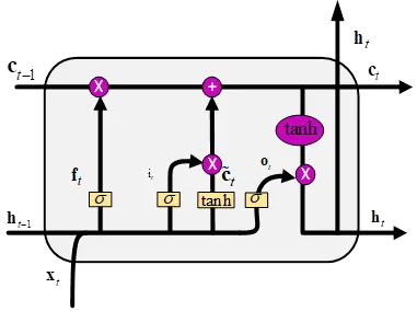The internal structure of the LSTM cell is given in Figure 1, which consists of the store cell $$\mathbf{c}_{t}$$, input gate $$\mathbf{i}_{t}$$, output gate $$\mathbf{o}_{t}$$ and forget gate $$\mathbf{f}_{t}$$. The cell unit is the core unit of the whole network and records the state of the network at the current moment. Three gates regulate the flow of information to the inputs and outputs of the memory cell and update the information stored in the cell through Equation (3):

```latex \begin{cases}\mathbf{i}_t=\sigma(\mathbf{W}_{hi}\mathbf{h}_{t-1}+\mathbf{W}_{xi}\mathbf{x}_t+\mathbf{W}_{ci}\odot\mathbf{c}_{t-1}+\mathbf{b}_i)\\\mathbf{f}_t=\sigma(\mathbf{W}_{hf}\mathbf{h}_{t-1}+\mathbf{W}_{xf}\mathbf{x}_t+\mathbf{W}_{cf}\odot\mathbf{c}_{t-1}+\mathbf{b}_f)\\\mathbf{\tilde{c}}_t=\tanh\left(\mathbf{W}_{hc}\mathbf{h}_{t-1}+\mathbf{W}_{xc}\mathbf{x}_t+\mathbf{b}_c\right)\\\mathbf{c}_t=\mathbf{f}_t\odot\tilde{\mathbf{c}}_{t-1}+\mathbf{i}_t\odot\tilde{\mathbf{c}}_t\\\mathbf{o}_t=\sigma(\mathbf{W}_{ho}\mathbf{h}_{t-1}+\mathbf{W}_{xo}\mathbf{x}_t+\mathbf{W}_{co}\odot\mathbf{c}_t+\mathbf{b}_o)\\\mathbf{h}_t=\mathbf{o}_t\odot\tanh\left(\mathbf{c}_t\right)&\end{cases} ```

(3)

where $$\mathbf{x}_{t}$$ is the input signal, $$\bigodot$$ represents Hadamard product, $$\mathbf{W}$$ is the weighting matrix (For example: $$\mathbf{W}_{x i}$$, $$\mathbf{W}_{h i}$$and $$\mathbf{W}_{c i}$$ represents the weight matrix of the input message to the input gate), $$\mathbf{b}$$ indicating bias (For example: $$\mathbf{b}_{i}$$ Indicates the bias of the input gate), $$\sigma$$ and $$\mathrm{t a n h}$$ is the activation function.

Figure 1. Hidden layer structure of LSTM.

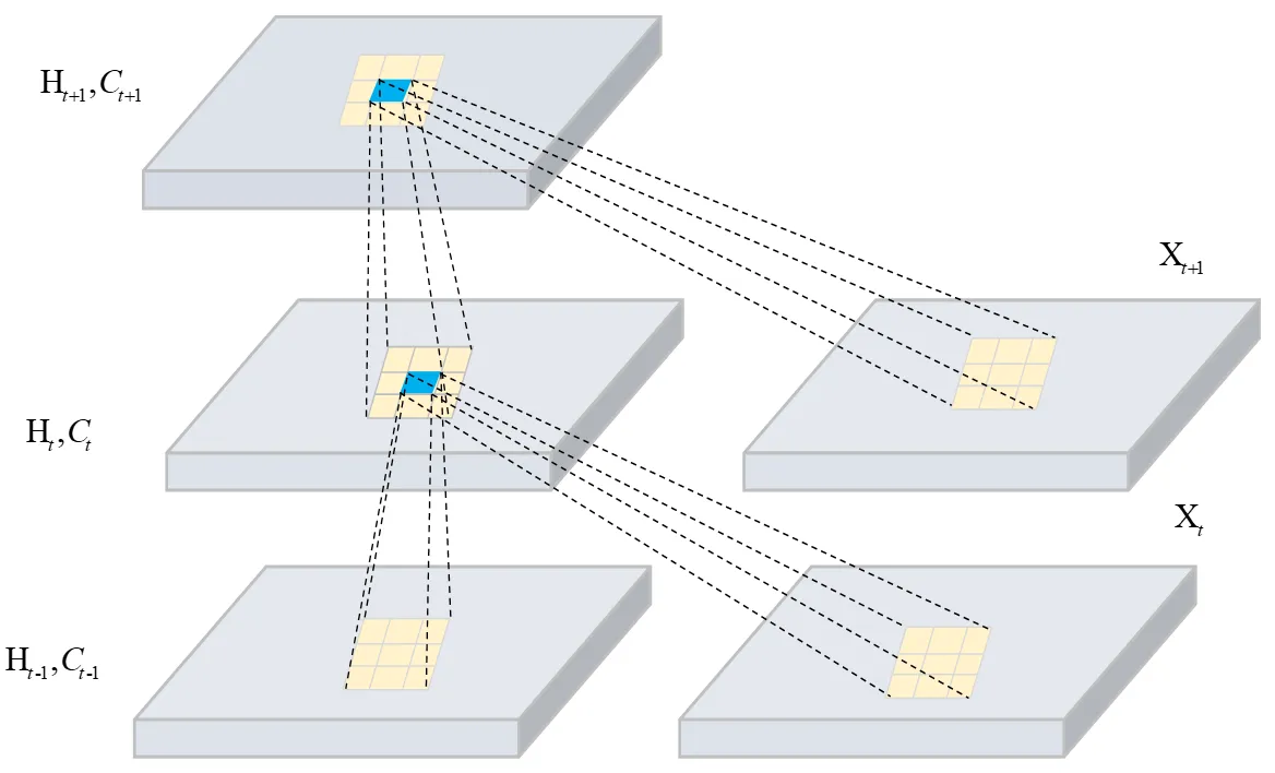
To effectively monitor the operating status of rolling bearings, time series data with high sampling frequency are obtained through sensors containing both time dependent and spatial localized features. LSTM can only focus on the time series features in the data when performing data prediction and cannot effectively extract the spatial features in the monitoring signals. This makes it difficult to capture the changing pattern of vibration signals in space, and these spatial features can often provide richer information than a single point-in-time feature, which can help to identify potential anomalies or malfunctions in a mechanical system more accurately. Therefore, the prediction accuracy of LSTM may be affected as a result. Convolutional long short-term memory network (CLSTM), as an improved LSTM method [49], combines the advantages of CNN and LSTM, which can effectively solve this challenge. Unlike traditional LSTM, CLSTM extracts spatial features in time series data by convolutional operations at each time step. In addition, CLSTM makes the network’s generalization ability more excellent by adding a convolution operation, which improves the prediction performance of the network. Figure 2 shows the structure of CLSTM, updating the state of its cells by the following equation:

Figure 2. CLSTM Structure.

Input gate $$\mathbf{Y}_{i}^{t}$$:

```latex \mathbf{A}_i^t=\mathbf{W}_{hi}∗\mathbf{H}_{t-1}+\mathbf{W}_{xi}∗\mathbf{X}_t+\mathbf{W}_{ci}\odot\mathbf{C}_{t-1}+\mathbf{B}_i ```

(4)

```latex \mathbf{Y}_i^t=\sigma(\mathbf{A}_i^t) ```

(5)

Forget gate $$\mathbf{Y}_{f}^{t}$$:

```latex \mathbf{A}_f^t=\mathbf{W}_{hf}^t∗\mathbf{H}_{t-1}+\mathbf{W}_{xf}∗\mathbf{X}_t+\mathbf{W}_{cf}\odot\mathbf{C}_{t-1}+\mathbf{B}_f ```

(6)

```latex \mathbf{Y}_f^t=\sigma(\mathbf{A}_f^t) ```

(7)

Memory cell $$\mathbf{Y}_{c}^{t}$$:

```latex \mathbf{A}_c^t=\mathbf{W}_{xc}∗\mathbf{X}_t+\mathbf{W}_{hc}∗\mathbf{H}_{t-1}+\mathbf{B}_c ```

(8)

```latex \mathbf{Y}_c^t=\mathbf{Y}_f^t\odot\mathbf{Y}_c^{t-1}+\mathbf{Y}_i^t\odot\tanh\left(\mathbf{A}_c^t\right) ```

(9)

Output gate $$\mathbf{Y}_{o}^{t}$$:

```latex \mathbf{A}_o^t=\mathbf{W}_{ho}∗\cdot\mathbf{H}_{t-1}+\mathbf{W}_{xo}∗\cdot\mathbf{X}_t+\mathbf{W}_{co}\odot\mathbf{Y}_c^t+\mathbf{B}_0 ```

(10)

```latex \mathbf{Y}_o^t=\sigma(\mathbf{A}_o^t) ```

(11)

Output $$\mathbf{H}_{o}^{t}$$:

```latex \mathbf{H}_o^t=\mathbf{Y}_o^t\odot\tanh{(\mathbf{Y}_c^t)} ```

(12)

where $$∗$$ is a convolution operation; $$\mathbf{W}_{h i}$$,$$\mathbf{W}_{x i}$$,$$\mathbf{W}_{c i}$$,$$\mathbf{W}_{h f}$$,$$\mathbf{W}_{x f}$$, $$\mathbf{W}_{c f}$$,$$\mathbf{W}_{h o}$$,$$\mathbf{W}_{x o}$$ and $$\mathbf{W}_{c o}$$ is the weight matrix of the corresponding gate in CLSTM, $$\mathbf{B}_{i}$$,$$\mathbf{B}_{f}$$ and $$\mathbf{B}_{o}$$ is the bias vector of the corresponding gate in CLSTM. 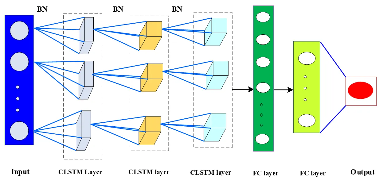3.2. ST-CNet Based Predictive Modeling Figure 3 shows the structure of the ST-CNet prediction model proposed in this paper, which extracts the implicit features in the HI by stacking 3-layer CLSTM layers, and then further inputs the extracted features into 2-layer fully-connected (FC) layers to expand the features into one-dimensional. The output layer is a linear regression layer, which is used to predict the degradation trend of the bearing. At the same time, batch normalization (BN) is added between each CLSTM layer to prevent the overfitting problem of ST-CNet.

Figure 3. Architecture of the proposed ST-CNet.

During the training process of ST-CNet, the gradient information about the loss function is calculated by the BPTT algorithm. Further, the Adaptive Moment Estimation (Adam) algorithm is used to update the network parameters of ST-CNet. Among them, the loss function is Mean Square Error (MSE), which is defined as follows:

```latex \mathrm{L(\theta)=\frac{1}{N}\sum_{i=1}^N(HI_i^{\prime}-HI_i)}^2 ```

(13)

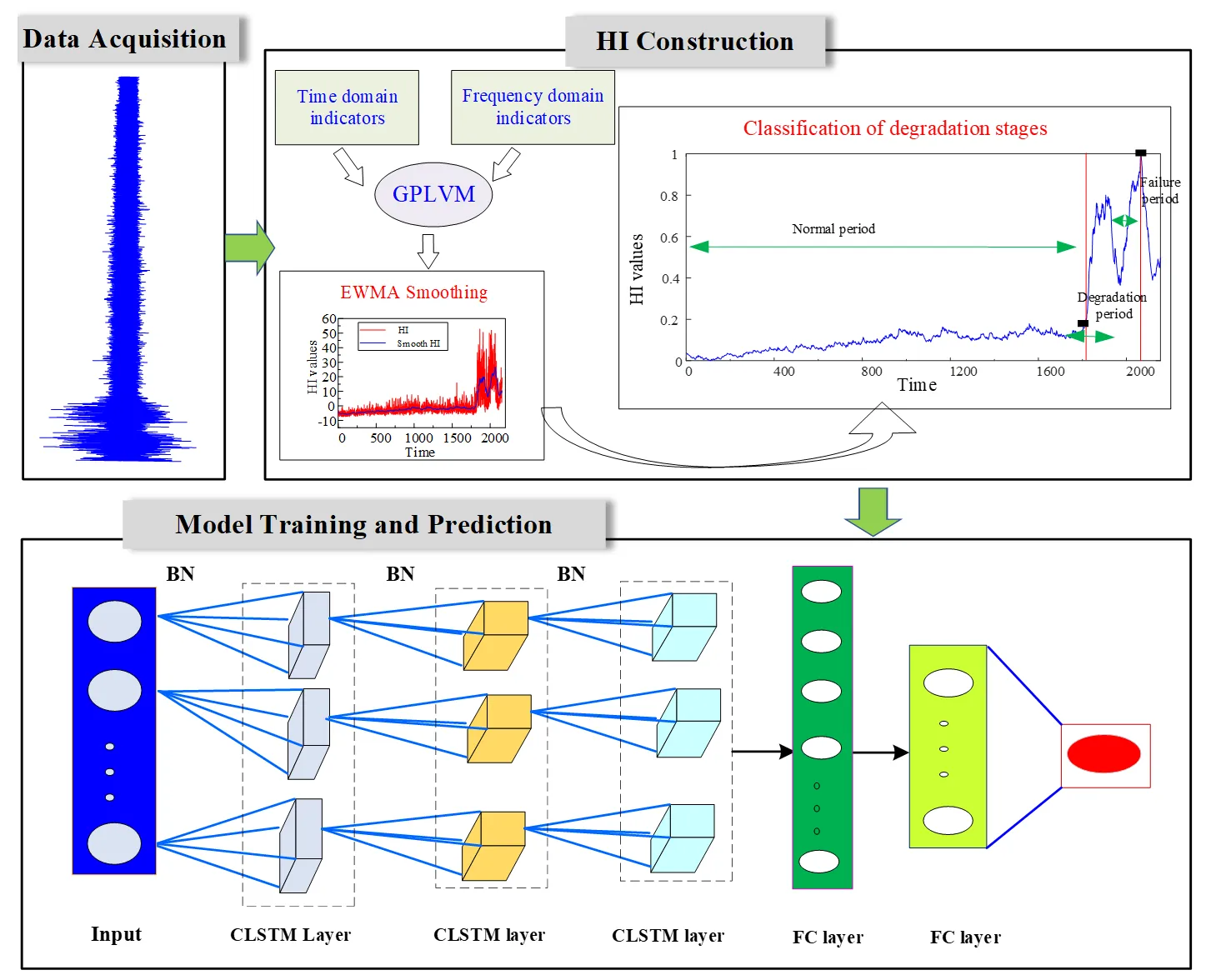
where $$\mathrm{H I_{i}}$$ represents the true value of the i-th HI, $$\mathrm{H I^{'}_{i}} $$ represents the HI value predicted by ST CNet, and N is the length of HI. 3.3. Degradation Trend Prediction Methodology Process In this paper, a rolling bearing degradation trend prediction method based on the multi-feature fusion health indicator and ST-CNet is proposed. The process is shown in Figure 4. First, multiple-domain features commonly used in practical engineering are extracted from the monitoring signals to form a feature dataset, and a new HI is designed to characterize the degradation state of rolling bearings by combining GPLVM and EMWA. Then, a new depth prediction model (i.e., ST-CNet) is constructed to predict the degradation trend of the rolling bearings by stacking multiple CLSTM layers. Finally, the measured data verifies the feasibility and superiority of the proposed method in this paper. The specific implementation steps of the proposed method are as follows:

(1): A vibration sensor is installed in the test bearing shell, and the accelerated life test is conducted under specific operating conditions to obtain the full-life data required for the test.
(2): Calculate the 16 time and frequency domain features, and use GPLVM to fuse the high-dimensional features and obtain the HI. After that, the extracted HI is smoothed using the EMWA algorithm with normalization, which obtains consecutive health indicators $$\mathbf{X}=[\mathrm{HI}_1,\mathrm{HI}_2,\cdotp\cdotp\cdotp,\mathrm{HI}_n]$$. Selecting the first m HI sequences $$\mathbf{X}_{\mathrm{train}}=[\mathrm{HI}_1,\mathrm{HI}_2,\cdotp\cdotp\cdotp,\mathrm{HI}_m]$$ as the training samples, the remaining HI sequences are used as test samples $$\mathbf{X}_{\mathrm{test}}=[\mathrm{HI}_{m+1},\mathrm{HI}_{m+2},\cdots,\mathrm{HI}_n]$$.
(3): Based on HIs, the performance degradation process of rolling bearings is divided into stages.
(4): The training samples are input into the ST-CNet model for training, and the multi-step prediction is used to predict the test samples. According to the prediction results, the future operation status of rolling bearings can be judged, which provides reference information for the subsequent company to arrange the maintenance plan. At the same time, to fairly assess the prediction performance of the model, this paper adopts the root mean squared error (RMSE) and mean absolute error (MAE) to assess the prediction performance of the model, and their mathematical expressions are as follows:

```latex \mathrm{RMSE}=\sqrt{\frac{1}{N}\sum_{i=1}^N(\mathrm{HI}_i-\mathrm{HI}_i^{\prime})^2} ```

(14)

```latex \mathrm{MAE}=\frac{1}{N}\sum_{i=1}^N\begin{vmatrix}\mathrm{HI}_i-\mathrm{HI}_i^{\prime}\end{vmatrix} ```

(15)

where $$N$$ denotes the length of the test sample. The smaller the values of RMSE and MAE, the higher the prediction accuracy of the prediction model.

Figure 4. Flow chart of degradation trend prediction method based on ST-CNet.

4. Experimental

This section conducts experiments based on the IMS bearing dataset to verify the feasibility and superiority of the proposed method, including health indicator extraction, degradation stage division, model parameter optimization, trend prediction, and comparative analysis. In this paper, the bearing dataset provided by IMS [50], a U.S. center for intelligent maintenance systems, is used to verify the feasibility of the proposed method. Figure 5 shows a rolling bearing accelerated life test rig consisting of four test bearings, a mechanical spring system and a motor. The mechanical spring system applies radial loads to the shaft and bearings, and the motor drives the test bearings to rotate.

Figure 5. Test rig of IMS [50].

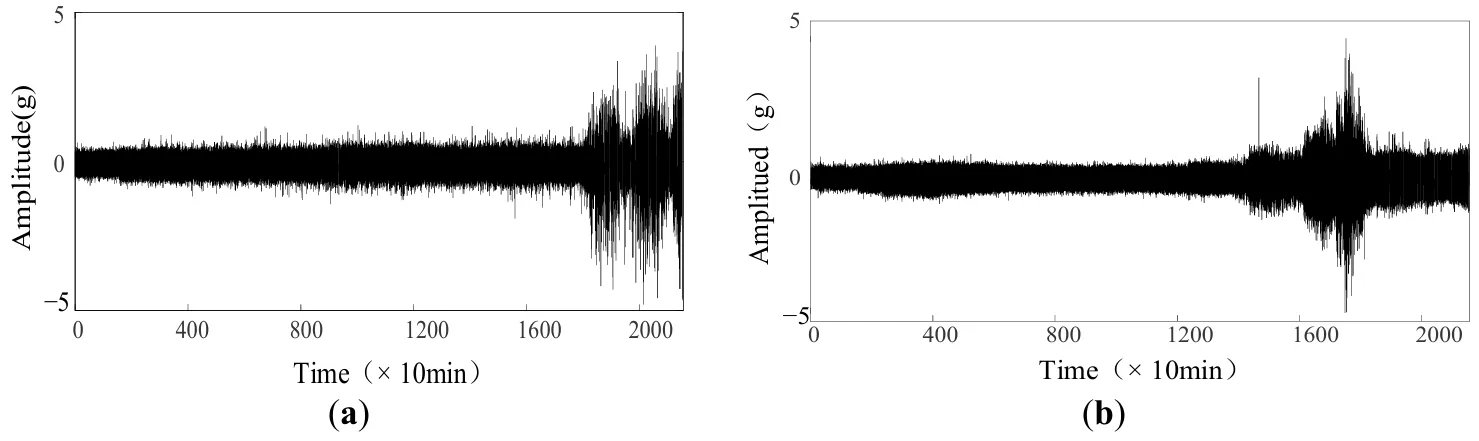
The rotational speed of the test bearing is 2000 rpm, the sampling frequency is 20 kHz, the sampling interval is 10 min, and its specific parameters are shown in Table 1. This paper selects the first group of experiments in the No. 3 bearing B3 (inner ring failure) and the No. 4 bearing B4 (rolling body failure) to be analyzed, and the time domain waveform is shown in Figure 6.

Table 1. Bearing parameters.

Circular Diameter	Rolling Element Diameter	Number of Rollers	Contact Ang
71.55 mm	8.4 mm	16	15.170

Figure 6. Time domain waveform of bearing life-cycle. (a) B3, (b) B4.

4.1. HI Extraction To describe the performance degradation process of rolling bearings more accurately and comprehensively, 16 kinds of statistical features are extracted from the vibration signals, respectively, which have different sensitivities to different types of bearing failures. Figure 7 gives the rolling bearing degradation trend graphs for the 16 features extracted from B4, and it can be seen that different features have different sensitivities to different stages of bearing degradation.

Figure 7. 16-dimensional features extracted from B4.

For example, $$t_{1}$$, $$t_{7}$$, $$f_{2}$$ and $$f_{4}$$ are affected by noise, with significant local fluctuations and a clear upward trend. The fluctuations of characteristics such as $$t_{2}$$, $$t_{4}$$, $$t_{8}$$, $$t_{10}$$, $$t_{11}$$ and $$t_{12}$$ are relatively small and sensitive to the accelerated degradation period of bearings, but the monotonic upward trend is not obvious. Each feature contains useful information about the bearing degradation process, and there is an obvious difference in the sensitivity of each feature to different degradation stages of the bearing. Therefore, it is necessary to extract multi-dimensional features to reflect the bearing degradation process. Although the above features can fully reflect the information in the bearing degradation process, the high-dimensional features will unavoidably have the problem of data redundancy. Next, the GPLVM algorithm is used to fuse the 16 extracted features to obtain a HI that can effectively characterize the bearing degradation process. The results are shown in Figure 8. It can be found that the HI curves of the two groups of data B3 and B4 show a degradation trend that first stays stable, then rises and then falls, which can roughly reflect the degradation process of bearings in the whole life cycle.

Figure 8. HI extraction. (a) B3, (b) B4.

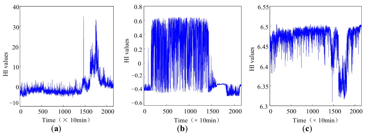
To verify the feasibility of the feature fusion through GPLVM, dimensionality reduction methods such as PCA, kernel principal component analysis (KPCA) and autoencoder were used to fit health indicators from B4. Among them, the Gaussian kernel function was used for KPCA, the number of hidden layers of the autoencoder was 3, and the number of training iterations was set to 30. It can be seen from Figure 9 that the HI constructed by KPCA and autoencoder methods has no obvious monotonic trend, and the HI obtained by the PCA method can reflect the degradation trend from normal to failure, but the local fluctuation of HI is larger. The monotonic trend of HI constructed by KPCA and autoencoder methods is not obvious, and the HI obtained by the PCA method can reflect the degradation trend of the bearing from normal to failure, but the local fluctuation of HI is large. Compared with the PCA method, GPLVM is a non-linear degradation method that can extract useful information from the non-linear high-dimensional space, and is more suitable for constructing the HI of rolling bearings.

Figure 9. HI fused by different dimension reduction methods. (a) PCA, (b) KPCA, (c) Autoencoder.

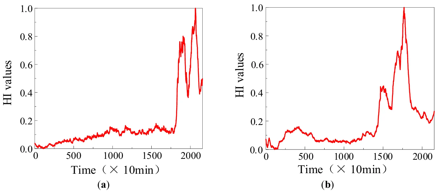
From Figure 8, it can also be seen that there are obvious partial fluctuations in HI, which will affect the accuracy of the model prediction if it is directly used for degradation trend prediction. Hence, the EWMA algorithm is used to smooth and normalize the HI, and the results are shown in Figure 10. As can be seen from the figure, the partial fluctuation in the HI is effectively filtered out, and a more reliable and monotonous HI is obtained to characterize the degradation process of rolling bearings.

Figure 10. HI after smoothing. (a) B3, (b) B4.

4.2. Classification of Degradation Stages The whole life cycle of rolling bearings is a long and gradually degenerative process, and it will go through different stages of degradation. Rolling bearings are in a healthy state of its run-to-failure time. Establishing a predictive model from normal times to predict its degradation trend is meaningless and difficult to judge the future operation state of rolling bearings accurately. Therefore, before predicting the degradation trend of rolling bearings, it is necessary to classify their degradation stages according to HI. In this paper, the HI is normalized. When the HI value is 1, it indicates that the current moment has reached the maximum failure threshold. Then, we can judge that the bearing has failed at the current moment. 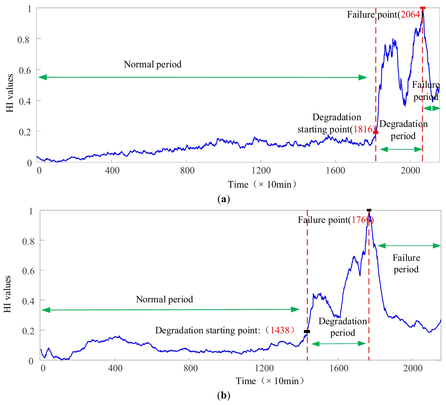Figure 11 shows the resultant plots of the two sets of signal degradation stage divisions. From Figure 11a, it can be seen that 0~18,150 min is the normal running time of B3. B3 after 18,160 min HI value gradually rises, bearing into the accelerated degradation stage. At this time, the HI value fluctuation occurs and the rolling bearing failure point in the impact of the gradual wear role becomes smooth. When HI value decreases, which is called the self-healing phenomenon. With the increased running time, the degree of bearing failure is further aggravated. When running to 20,640 min, the HI value is 1, indicating the rolling bearing is at a serious failure at the current time. Therefore, the period of time from 18,160 min to 20,640 min is classified as the degradation period of B3. In the period of 20,650 min~21,560 min, the HI value decreases, indicating that B3 has entered the failure period. From Figure 11b, it can be seen that the HI of B4 fluctuates from 0 to 14,370 min due to noise, but the range of fluctuation is small, so this period is the normal period of B4. After 14,380 min, the HI value of B4 rises gradually, and the bearing enters the accelerated degradation stage until the HI value is 1 at 17,690 min, indicating that the bearing reaches the failure threshold at the present moment. Therefore, 14,380 min~17,690 min is the degradation period of B4, and 17,700 min~21,560 min is the failure period of B4 with a decreasing trend of HI value.

Figure 11. Degradation stage division. (a) B3, (b) B4.

4.3. Determination of Key Parameters for Predictive Models

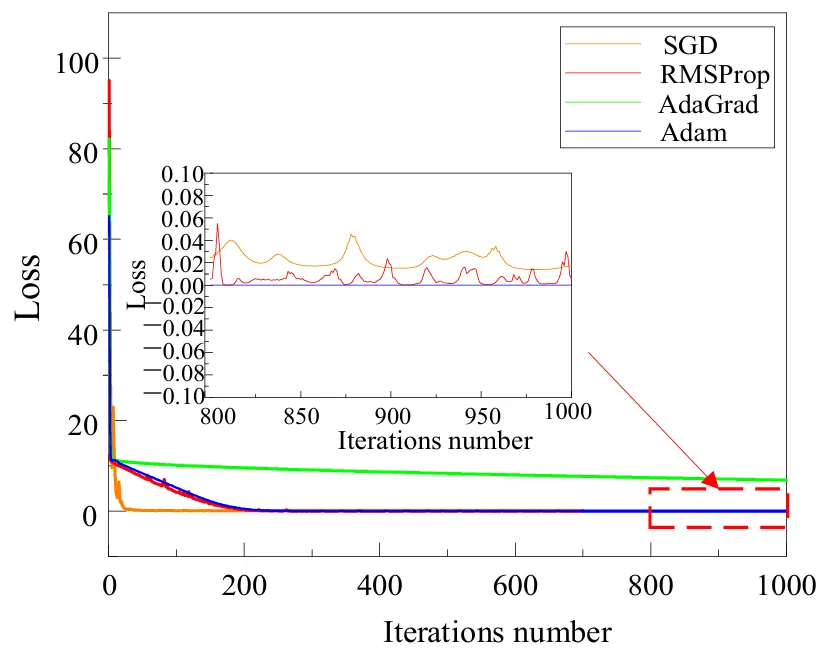
(1): Optimizer selection: An appropriate optimizer can not only improve the prediction accuracy of the network, but also accelerate the convergence speed of the network. Therefore, four commonly used optimizers, Adam, Root Mean Square Propagation (RMSProp), Adaptive Gradient Algorithm (AdaGrad) and Stochastic Gradient Descent (SGD) are selected to compare the prediction performance of the proposed ST-CNet. First, to explore the effect of different optimizers on the prediction performance of ST-CNet, the prediction error versus the number of iterations when different optimizers perform prediction is given in Figure 12. It can be seen that the loss value of AdaGrad is larger than that of the other optimizers after smoothing, indicating that the prediction error is larger. RMSProp and SGD show a certain degree of fluctuation in the Loss value when the number of iterations is 800~1000. Adam tends to stabilize when the number of iterations ranges from 800 to 100, and the Loss values are smaller than those of the other three optimizers, which indicates that Adam has more stable prediction performance when used as an optimizer for ST-CNet.
(2): Choice of number of iterations: The number of iterations is another important parameter in ST-CNet, and a suitable number of iterations can not only achieve better prediction results and reduce the model training time. In the experiment, the initial iteration number of ST-CNet is set to 1000 times, and the relationship between loss and iteration number is shown in Figure 12. The following conclusions can be drawn: (a) As the number of iterations increases, the prediction error of the model decreases and the accuracy of the prediction is higher. (b) The increase in the number of iterations also increases the training time of the model and even leads to the overfitting problem of the model. (c) When the number of iterations is 300, the loss value tends to stabilize, and its value is close to 0. The iterative updating of the model is no longer meaningful, so the number of iterations of ST-CNet is set to 300 times.

Figure 12. Relationship between the loss of different optimizers and iterations number.

4.4. Forecast of Degradation Trends The degradation period is a critical stage during the service life of bearings, and accurate prediction of the degradation trend at this stage can arrange a reasonable time for bearing replacement or repair to avoid accidents. For B3 data, the HI from 0 to 18,150 min is used to train ST-CNet, and then the HI values from 18,160~20,640 min are predicted. Similarly, the HI values of 0~14,370 min in B4 were used as training samples, and ST-CNet predicted the HI values of 14,380~17,690 min. 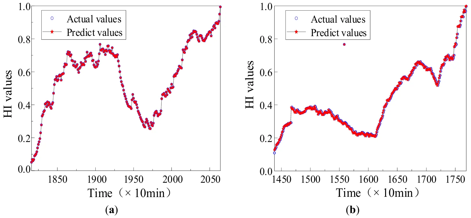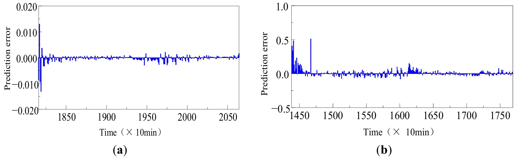Figure 13 gives the prediction results of B3 and B4, two data groups in the degradation period. It can be seen that the proposed method can accurately predict the degradation trend of rolling bearings, and the predicted HI value is very close to the true HI value. At the same time, the error between the real HI value and the predicted HI value is calculated by Equation (16). It can be seen in Figure 14 that the proposed ST-CNet has achieved a small prediction error when predicting the HI of B3 and B4 degradation period. Based on the above analysis, it can be seen that it is feasible to use the proposed method for the prediction of the degradation trend of rolling bearings, and the prediction accuracy is high.

```latex \mathrm{E_{e r r o r} = \frac{H I - H I^{'}}{H I}}```

(16)

where HI is the true value, $$\mathrm{H I^{\prime}}$$ denotes the predicted value of ST-CNet.

Figure 13. Degradation trend prediction results. (a) B3, (b) B4.

Figure 14. Prediction error. (a) B3, (b) B4.

4.5. Comparative Experimental Analysis To verify the applicability of the HI constructed in this paper in the prediction of rolling bearing degradation trend, we compared it with the HI constructed by other methods, and the results are shown in Table 2. Four state-of-the-art data-driven models are selected for comparison, with their structures and parameters strictly consistent with their original literature to ensure fairness: 1. BPNN: A 3-layer backpropagation neural network with 64 neurons in the hidden layer, optimized by genetic algorithm (learning rate = 0.01, batch size = 32). It lacks the ability to model temporal dependencies, limiting its performance on time-series degradation data. 2. LSTM: A single-layer LSTM with 128 memory units, using Adam optimizer (learning rate = 0.001). It captures long-term temporal dependencies but cannot extract spatial features from vibration signals. 3. GRU: A simplified variant of LSTM with 64 hidden units (learning rate = 0.001), reducing computational complexity by merging input and forget gates. However, it still ignores spatial correlations in data. 4. Bi-LSTM: A bidirectional LSTM with 128 units in both forward and backwards layers (learning rate = 0.001), capturing temporal features in both past and future directions but remaining deficient in spatial feature extraction.The table shows that when the HI constructed in this paper is used to input to ST-CNet for prediction, smaller MAE and RMSE values are achieved, which means that it has a smaller prediction error.

Table 2. Comparison results of different HI prediction performance.

Different HI	B3		B4
Different HI	MAE	RMSE	MAE	RMSE
Mean	0.159	0.237	0.115	0.116
Time Frequency	0.176	0.176	0.047	0.048
Proposed HI	0.093	0.091	0.012	0.013

In addition, to verify that the proposed ST-CNet has better prediction performance, it is compared with some published state-of-the-art methods, including BPNN, LSTM, GRU and Bi-LSTM. In the experiments, the HI extracted in this paper is input to each comparison method for prediction, and the results are shown in Figure 15. Figure 15a shows the results of each comparison method for predicting the HI value of B3 at 18,160~20,640 min. It can be seen that the predicted HI value of the proposed method is the closest to the real HI value, and the prediction accuracy is better than that of other comparison methods. Figure 15b shows the results of comparing the HI values predicted by each comparison method for B4 in the range of 14,380~17,690 min. From the figure, it can be found that the prediction accuracy of BPNN is the worst, the prediction performance of Bi-LSTM is better than GRU’s, and GRU’s prediction performance is better than LSTM’s.

Figure 15. HI prediction results of different methods. (a) B3, (b) B4.

To measure the prediction performance of the comparison methods in a comprehensive way, the MAE and RMSE values of each comparison method for prediction are calculated separately. It can be found from the Table 3 that the proposed method achieves smaller MAE and RMSE values in both B3 and B4, which further indicates that the method proposed in this paper has higher prediction accuracy. Based on the above analysis results, the proposed ST-CNet has better prediction performance than the published methods.

Table 3. Evaluation index results of different methods on IMS data.

Method	B3		B4
Method	MAE	RMSE	MAE	RMSE
BPNN [29]	0.541	0.586	0.386	0.434
LSTM [33]	0.232	0.258	0.208	0.259
GRU [34]	0.206	0.236	0.133	0.161
Bi-LSTM [35]	0.155	0.174	0.074	0.093
Proposed method	0.093	0.091	0.012	0.013

The experimental results show that the proposed HI and ST-CNet achieve high prediction accuracy (Table 2 and Table 3), consistent with the view that multi-feature fusion and spatio-temporal modeling improve degradation assessment. Notably, the non-linear feature extraction capability of GPLVM and the smoothing effect of EWMA effectively suppress noise interference, which aligns with the conclusion that robust health indicators are critical for capturing subtle degradation trends. In practical industrial scenarios, rolling bearing degradation is often intertwined with the operational state of supporting systems. For instance, the biological instability of metalworking fluids—caused by microbial contamination—can accelerate bearing wear by altering lubrication properties. With its high sensitivity to early degradation (Figure 13), the proposed method can indirectly reflect potential issues in auxiliary systems like metalworking fluid management. This linkage bridges mechanical degradation prediction and fluid maintenance, providing a holistic perspective for equipment health management.

5. Conclusions

(1): Distinct from traditional single-feature or linear dimensionality reduction-based health indicator (HI) construction methods, this work uniquely integrates 16 time-frequency domain features to form a multi-dimensional dataset. By leveraging the Gaussian Process latent variable model (GPLVM) for non-linear dimensionality reduction, a novel HI is constructed to characterize the bearing degradation process comprehensively. Further, the exponentially weighted moving average (EWMA) is employed to smooth the HI, effectively filtering out noise-induced local fluctuations—this two-step fusion and smoothing strategy addresses feature redundancy and non-linearity issues in HI construction, a key innovation here.
(2): Unlike conventional data-driven models that lack the ability to capture spatial features, the proposed ST-CNet innovatively combines convolutional long short-term memory (CLSTM) layers to fully exploit spatiotemporal characteristics in monitoring data. This design enables the model to simultaneously extract local spatial patterns and long-term temporal dependencies, thus enhancing the accuracy of degradation trend prediction.
(3): Experimental results confirm that the proposed method achieves the minimum MAE and RMSE compared to state-of-the-art methods, validating its superior performance in rolling bearing degradation trend prediction. The application case based on the IMS dataset demonstrates that the method is feasible for integration into practical condition monitoring systems, providing reliable degradation trend insights to support equipment maintenance decisions. This work offers an effective rolling bearing health management solution, contributing to improved equipment reliability and safety.

Author Contributions

G.H. and N.W., conceptualization, methodology, writing—original draft; S.W. and Q.W., formal analysis, visualization; W.W., L.L. and Y.F., supervision and writing—review and editing. All authors have read and agreed to the published version of the manuscript.

Ethics Statement

Not applicable.

Informed Consent Statement

Not applicable.

Data Availability Statement

Not available.

Funding

Declaration of Competing Interest

The authors declare that there are no know conflicts of financial interests and it has not been published in other journals.

References

Lan X, Li Y, Su Y, Meng L, Kong X, Xu T. Performance degradation prediction model of rolling bearing based on self-checking long short-term memory network. Meas. Sci. Technol. 2023, 34, 015016. doi:10.1088/1361-6501/ac9a2a. [Google Scholar]

Liu H, Yuan R, Lv Y, Yang X, Li H, Song G. Degradation tracking of rolling bearings based on local polynomial phase space warping. IEEE Trans. Reliab. 2023, 73, 1380–1392. doi:10.1109/TR.2023.3266110. [Google Scholar]

Zhang Y, Peng Y, Liu L. Degradation estimation of electromechanical actuator with multiple failure modes using integrated health indicators. IEEE Sens. J. 2020, 20, 7216–7225. doi:10.1109/JSEN.2020.2978284. [Google Scholar]

Yan T, Wang D, Sun S, Shen C, Peng Z. Novel sparse representation degradation modeling for locating informative frequency bands for machine performance degradation assessment. Mech. Syst. Signal Process. 2022, 179, 109372. doi:10.1016/j.ymssp.2022.109372. [Google Scholar]

Chen B, Song D, Cheng Y, Zhang W, Huang B, Muhamedsalish Yousif. IGIgram: An improved Gini index-based envelope analysis for rolling bearing fault diagnosis. J. Dyn. Monit. Diagn. 2022, 1, 111–124. doi:10.1007/s43684-022-00031-5. [Google Scholar]

Yan T, Wang D, Zheng M, Xia T, Pan E, Xi L. Fisher’s discriminant ratio based health indicator for locating informative frequency bands for machine performance degradation assessment. Mech. Syst. Signal Process. 2022, 162, 108053. doi:10.1016/j.ymssp.2021.108053. [Google Scholar]

Gu Y, Bi Q, Qiu G. Practical health indicator construction methodology for bearing ensemble remaining useful life prediction with ISOMAP-DE and ELM-WPHM. Meas. Sci. Technol. 2021, 32, 25007. doi:10.1088/1361-6501/abc5c1. [Google Scholar]

Chen D, Qin Y, Wang Y, Zhou J. Health indicator construction by quadratic function-based deep convolutional auto-encoder and its application into bearing RUL prediction. ISA Trans. 2021, 114, 44–56. doi:10.1016/j.isatra.2021.01.045. [Google Scholar]

Smith RA, Liu C. Advances in Understanding Rolling Contact Fatigue Mechanisms. J. Tribol. 2024, 146, 021401. doi:10.1115/1.4064600. [Google Scholar]

10.

Wang J, Zhao Y, Guo W, Ji D, Wang L, Yang Z, et al. Research Progress on the Failure Mechanisms of Rolling Contact Fatigue. Tribol. Int. 2023, 182, 107231. doi:10.1016/j.triboint.2023.107231. [Google Scholar]

11.

Voskamp AP, Mittemeijer EJ. State of residual stress induced by cyclic rolling contact loading. Mater. Sci. Technol. 1997, 13, 430–438. doi:10.1179/mst.1997.13.5.430. [Google Scholar]

12.

Li S, Zhang J, Wang H, Chen X, Liu Yet. Relationship between Residual Stress and Fatigue Performance in Bearing Materials. J. Mater. Eng. Perform. 2024, 33, 3047–3057. doi:10.1007/s11665-024-09372-1. [Google Scholar]

13.

Liu X, Zhang Y, Li Z. Inducing Residual Stress through Hard Turning for Bearing Components. Int. J. Mach. Tools Manuf. 2023, 189, 104186. doi:10.1016/j.ijmachtools.2023.104186. [Google Scholar]

14.

Chen Y, Wang Z, Zhao W. Deep Rolling—Induced Residual Stress Profiles in Bearing Steel. Surf. Coat. Technol. 2024, 474, 130044. doi:10.1016/j.surfcoat.2024.130044. [Google Scholar]

15.

Zhao X, Hu Q, Chen L, Zhou M, Zhang K. The Role of Compressive Residual Stress in Delaying Fatigue Crack Growth in Rolling Bearings. Fatigue Fract. Eng. Mater. Struct. 2025, 48, 1265–1278. doi:10.1111/ffe.14025. [Google Scholar]

16.

Sun W, Li R, Xu T, Wu H, Liu J. Influence of Sub—surface Compressive Residual Stress on the Fatigue Life of Rolling Contact. Tribol. Trans. 2024, 67, 541–550. doi:10.1080/10402004.2024.2346781. [Google Scholar]

17.

Xia Z, Wu D, Zhang X, Wang J, Han E. Rolling Contact Fatigue Failure Mechanism of Bearing Steel on Different Surface Roughness Levels Under Heavy Load. Int. J. Fatigue 2024, 182, 107310. doi:10.1016/j.ijfatigue.2024.107310. [Google Scholar]

18.

Pape F, Neubauer T, Maiß O, Denkena B, Poll G. Influence of residual stresses introduced by manufacturing processes on bearing endurance time. Tribol. Lett. 2017, 65, 70. doi:10.1007/s11249-017-0838-4. [Google Scholar]

19.

Denkena B, Poll G, Maiß O, Pape F, Neubauer T. Enhanced boundary zone rolling contact fatigue strength through hybrid machining by hard turn-rolling. Bear. World J. 2016, 1, 87–102. [Google Scholar]

20.

Wang Y, Liu C, Huang Z, Zhang P, Wei Q, Li F. Development of Health Indicators for Rolling Bearings Based on Residual Stress Analysis. Mech. Syst. Signal Process. 2025, 192, 109572. doi:10.1016/j.ymssp.2025.109572. [Google Scholar]

21.

Zhang L, Yang T, Zhou X, Xu R, Li H, Wang M. Prediction Models for Rolling Bearing Degradation Considering Residual Stress and Surface Roughness. Reliab. Eng. Syst. Saf. 2024, 245, 108624. doi:10.1016/j.ress.2024.108624. [Google Scholar]

22.

Lei Y, Li N, Gontarz S, Lin J, Radkowski S, Dybala J. A model-based method for remaining useful life prediction of machinery. IEEE Trans. Reliab. 2016, 65, 1314–1326. doi:10.1109/TR.2016.2519918. [Google Scholar]

23.

Hu C, Youn BD, Wang P. Ensemble of data-driven prognostic algorithms for robust prediction of remaining useful life. Reliab. Eng. Syst. Saf. 2012, 103, 120–135. doi:10.1016/j.ress.2011.12.008. [Google Scholar]

24.

Kumar P, Kumaraswamidhas L, Laha S. Selection of efficient degradation features for rolling element bearing prognosis using Gaussian Process Regression method. ISA Trans. 2021, 112, 386–401. doi:10.1016/j.isatra.2021.01.033. [Google Scholar]

25.

Cui L, Wang X, Wang H, Ma J. Research on remaining useful life prediction of rolling element bearings based on time-varying kalman filter. IEEE Trans. Instrum. Meas. 2020, 69, 2858–2867. doi:10.1109/TIM.2019.2956412. [Google Scholar]

26.

Li X, Zhang W, Ding Q. Deep learning-based remaining useful life estimation of bearings using multi-scale feature extraction. Reliab. Eng. Syst. Saf. 2019, 182, 208–218. doi:10.1016/j.ress.2018.11.002. [Google Scholar]

27.

Xia M, Li T, Shu T, Wan J, De Silva C, Wang Z. A two-stage approach for the remaining useful life prediction of bearings using deep neural networks. IEEE Trans. Ind. Inform. 2019, 15, 3703–3711. doi:10.1109/TII.2018.2886792. [Google Scholar]

28.

Cheng C, Ma G, Zhang Y, Sun M, Teng F, Ding H, et al. A deep learning-based remaining useful life prediction approach for bearings. IEEE/ASME Trans. Mechatron. 2020, 25, 1243–1254. doi:10.1109/TMECH.2020.2975008. [Google Scholar]

29.

Yang L, Wang J. GA-BP Algorithm Predicts the Degrading Trend of Rolling Bearings. In Proceedings of the 2021 IEEE International Conference on Sensing, Diagnostics, Prognostics, and Control (SDPC), Weihai, China, 13–15 August 2021; pp. 69–73.

30.

Guo L, Li N, Jia F, Lei Y, Lin J. A recurrent neural network based health indicator for remaining useful life prediction of bearings. Neurocomputing 2017, 240, 98–109. doi:10.1016/j.neucom.2017.02.053. [Google Scholar]

31.

Hochreiter S, Schmidhuber J. Long short-term memory. Neural. Comput. 1997, 9, 1735–1780. doi:10.1162/neco.1997.9.8.1735. [Google Scholar]

32.

Cho K, Van Merriënboer B, Gulcehre C, Bahdanau D, Bougares F, Schwenk H, et al. Learning phrase representations using RNN encoder-decoder for statistical machine translation. arXiv 2014, arXiv:1406.1078. doi:10.48550/arXiv.1406.1078.

33.

Hu Y, Wei R, Yang Y, Li X, Huang Z, Liu Y, et al. Performance degradation prediction using LSTM with optimized parameters. Sensors 2022, 22, 2407. doi:10.3390/s22062407. [Google Scholar]

34.

Zheng X, Qian Y, Wang S. GRU prediction for performance degradation of rolling bearings based on optimal wavelet packet and Mahalanobis distance. J. Vib. Shock. 2020, 39, 39–49. [Google Scholar]

35.

Huang C, Huang H, Li Y. A Bidirectional LSTM prognostics method under multiple operational conditions. IEEE Trans. Ind. Electron. 2019, 66, 8792–8802. doi:10.1109/TIE.2018.2886783. [Google Scholar]

36.

Wang Y, Liu C, Huang Z, Zhang P, Wei Q, Li F. A Review of Health Indicator Construction for Rolling Bearing Degradation Assessment. Mech. Syst. Signal Process. 2024, 190, 109431. doi:10.1016/j.ymssp.2024.109431. [Google Scholar]

37.

Liu Z, Zhang R, Chen D, Wu X, Zhou Y, Zhao. Challenges and Opportunities in Bearing Degradation Prediction: A State-of-the-Art Review. J. Mech. Eng. Sci. 2025, 239, 1167–1189. doi:10.1177/09544062241234567. [Google Scholar]

38.

Zhao H, Wang J, Xu M, Sun T, Li H, Zhang L, et al. Research Progress on Data—Driven Health Monitoring and Prognosis of Rolling Bearings. Tribol. Int. 2024, 187, 107635. doi:10.1016/j.triboint.2023.107635. [Google Scholar]

39.

He X, Guo S, Feng Z, Jiang W, Lin J. Non-linear Feature Extraction and Health Indicator Construction for Bearing Degradation Monitoring. IEEE Trans. Instrum. Meas. 2023, 72, 5000712. doi:10.1109/TIM.2023.3291234. [Google Scholar]

40.

Chen X, Zhou Y, Liu J, Tang H, Zhang Q, Mao Y. Improving the Monotonicity and Non-linearity of Health Indicators for Bearing Prognosis Using Advanced Feature Fusion. Measurement 2024, 205, 112765. doi:10.1016/j.measurement.2024.112765. [Google Scholar]

41.

Zhang L, Yang T, Zhou X, Xu R, Li H, Wang M. Non-linear Degradation Modeling of Rolling Bearings Considering Complex Operating Conditions. J. Vib. Acoust. 2025, 147, 031012. doi:10.1115/1.4064601. [Google Scholar]

42.

Qiu N, Huang F, Ye L, Lu B, Song K. Spatio-temporal Feature Learning for Bearing Degradation Prediction: A Comparative Study. Mech. Syst. Signal Process. 2024, 193, 109634. doi:10.1016/j.ymssp.2024.109634. [Google Scholar]

43.

Li Y, Sun W, Jiang R, Hu Z, Liang S, Wang G. Integrating Spatial and Temporal Information for Bearing Fault Diagnosis and Prognosis: A Review. IEEE Access 2023, 11, 107442–107462. doi:10.1109/ACCESS.2023.3291234. [Google Scholar]

44.

Wang Y, Jiang Y, Kang S. The applications of time domain and frequency domain statistical factors on rolling bearing performance degradation assessment. Comput. Model. New Technol. 2014, 18, 192–198. [Google Scholar]

45.

Qiu G, Gu Y, Chen J. Selective health indicator for bearings ensemble remaining useful life prediction with genetic algorithm and Weibull proportional hazards model. Measurement 2020, 150, 107097. doi:10.1016/j.measurement.2019.107097. [Google Scholar]

46.

Zhou F, Park JH, Liu Y. Differential feature based hierarchical PCA fault detection method for dynamic fault. Neurocomputing 2016, 202, 27–35. doi:10.1016/j.neucom.2016.01.058. [Google Scholar]

47.

Li P, Chen S. A review on Gaussian process latent variable models. CAAI Trans. Intell. Technol. 2016, 1, 366–376. doi:10.1049/trit.2016.0010. [Google Scholar]

48.

Li X, Jiang H, Xiong X, Shao H. Rolling bearing health prognosis using a modified health index based hierarchical gated recurrent unit network. Mech. Mach. Theory 2019, 133, 229–249. doi:10.1016/j.mechmachtheory.2018.12.021. [Google Scholar]

49.

Trifa A, Sbai AH, Chaari WL. Enhancing assessment of personalized multi-agent system through convlstm. Procedia Comput. Sci. 2017, 112, 249–259. doi:10.1016/j.procs.2017.08.256. [Google Scholar]

50.

Li G, Wei J, He J, Yang H, Meng F. Implicit Kalman filtering method for remaining useful life prediction of rolling bearing with adaptive detection of degradation stage transition point. Reliab. Eng. Syst. Saf. 2023, 235, 109269. doi:10.1016/j.ress.2023.109269. [Google Scholar]