1. Introduction
Climate warming has intensified the hydrologic cycle, increasing the frequency and intensity of heavy-precipitation events in many, though not all, regions [
1,
2,
3,
4]. Recent studies confirm this trend into the 2020s, particularly for sub-daily extremes [
5,
6,
7].Where such extremes have grown, flood hazards often rise as well [
8], yet observed changes in flood magnitude and frequency have not been consistent across the United States [
9,
10,
11,
12,
13]. The extent of change depends on geographic setting, for example, inland versus coastal areas (climate nonstationarity) [
14,
15,
16] or on basin characteristics, such as rural versus urbanized catchments (anthropogenic nonstationarity) [
17,
18,
19]. As such, flood quantile estimates reflecting nonstationarity arising from climate or human influences can help reduce flood hazards [
20].
Considerable effort has gone into estimating flood quantiles at both regional [
17,
21,
22,
23,
24,
25] and national scale [
26,
27,
28] across the conterminous United States. Collins [
22] found that nonstationary behavior in flood series appeared as a step change in the long-term mean for undisturbed basins in New England and recommended separate flood frequency analyses for periods before and after the change point. Because these basins are minimally affected by human activities, their flood frequency changes mainly reflect climate variability. In the eastern [
25] and midwestern [
29] United States, studies of basins with documented anthropogenic disturbances including land use/cover change (e.g., urbanization, forest harvest), agriculture and subsurface drainage, river regulation and reservoir construction, groundwater pumping, channelization or levee construction revealed step changes in long-term average peak flow driven by both climate variability and human activities.
Analyzing at least 15 to 25 years of instrumental records is essential for identifying spatiotemporal patterns in hydrologic variables [
30] When flood series are split into periods before and after a change point, enough observations must remain for reliable analysis, particularly for floods with 100 years or longer return periods. This study examined reference and non-reference basins [
31,
32] with more than 100 years of peak flow data nationwide. Change points in the long-term mean of annual peak flow series were detected using the nonparametric Pettitt test [
33], and observations were partitioned into two clusters before and after the change point. We selected the Pettitt test because it remains competitive with multiple-change algorithms for single shift detection in hydrologic time series [
34]. The Log Pearson Type III (LP3) distribution was then fitted to each cluster and the entire period of record to derive flood quantile estimates. Parameter estimates followed the Bulletin 17C guidelines [
35], incorporating product moment and L-moment variants.
This study shows that nonstationarity in long-term mean peak flow behaves differently at reference sites, where changes mainly reflect climate variability and at non-reference sites, where local human actions also play a role. At non-reference gages, basin alterations such as urbanization, land-cover change, dam construction, and river regulation can dampen or even counteract the climate-driven signal observed at minimally disturbed sites. Recognizing this contrast helps analysts decide whether flood quantile estimates should be drawn from the entire record or pre- and post-change segments, thereby reducing bias in design values.
2. Materials and Methods
2.1. Change Point Detection
A time series may exhibit one or more shifts in its long-term mean, so-called change points or regime shifts [
36]. A change point represents a transition from one mean state to a higher or lower one, confirmed when the difference between the two states is statistically significant. Several techniques exist for detecting single [
33] or multiple [
36] change points. Although identifying multiple shifts can help distinguish among different forms of nonstationarity, partitioning the data into many segments reduces the sample size and can limit meaningful flood frequency analysis, especially for extreme events with longer return periods.
On the other hand, while changes in variance, skewness, or monotonic trend can also indicate nonstationarity, our primary objective is to identify discrete shifts in the mean that most directly affect LP3 quantiles [
37]. Variance-shift tests and trend-based models demand longer post-split samples than are available for many gages [
38].We applied the nonparametric Pettitt test [
33]. to detect a single shift in each stream gage flood data series. The sequential test requires no prior knowledge of the shift’s timing. Because it is nonparametric, the Pettitt test is less sensitive to skewed data than parametric alternatives [
25,
39]. When a shift was statistically significant (
p-value ≤ 0.05), the flood record was split into two periods before and after the change point for separate flood frequency analyses. All change-point analyses were performed with the “trend” package in R programing language software [
40].
2.2. Flood Quantiles Estimate
Flood frequency analysis was performed with the LP3 distribution [
35,
41]. The shape, scale, and location parameters of LP3 have been well documented [
42,
43,
44,
45]. We adopted the product moment formulation of Stedinger et al. [
46] and applied no bios correction for station skewness. Taking the natural logarithm from the peak flow observations “$$X = \mathcal{l} n \left(Q\right)$$”, the Probability Density Function (PDF) of the LP3 distribution can be defined as:
For a sample of “
n” log-transformed peak flow observations, three sample moments of mean ($$\hat{\mu}_{X}$$, first moment), variance ($$\hat{\sigma}^{2}_{X}$$, second moment), and skewness ($$\hat{\gamma}_{X}$$, third moment) can be calculated as below:
The LP3 shape ($$\alpha$$), scale ($$\beta$$), and location ($$\xi$$) parameters follow [
46] which help find the moments of LP3 distribution,
i.e., $$\mu_{Q}$$, $$\sigma_{Q}^{2}$$, and $$\gamma_{Q}$$:
The peak flow can be estimated at certain quantiles “
P” [
47] using:
The frequency factor $$K_{P} \left(\gamma_{Q}\right)$$ can be computed by the Wilson-Hilferty formula valid for $$0 . 01 \leq P \leq 0 . 99$$ and $$\left|\gamma\right| < 2$$ [
46,
47]. The $$Z_{P}$$, the
Pth quantile of the standard normal distribution with zero mean and one standard deviation is estimated by [
48]:
The exceedance probability for descending ordered peak flow observations (
i = 1 for the largest observation) is calculated using the Blom formula [
45]:
The Blom formula assigns the return period of $$T = 1 . 6 n + 0 . 4$$ to the largest observation [
46] and thus yields a return period of about 160 years for sample size of $$n = 100$$ years or more. Goodness of fit was evaluated by plotting frequency factor $$K_{P_{i}} \left(\gamma_{Q}\right)$$ versus standardized observations $$Z_{i} = \frac{X_{i} - \overset{-}{X}}{\sigma_{X}}$$ and verifying alignment with the 1:1 line [
44]. The distribution-based frequency factor $$K_{P_{i}} \left(\gamma_{Q}\right)$$ was computed from Equation (5), whereas the observation-based $$Z_{P}$$ from Equation (6). All calculations were implemented in R [
49]. Authors custom code for the LP3 fitting and diagnostics follows the algorithms described above. A detailed LP3 performance assessment workflow is provided later in the results section.
3. Data
The U.S. Geological Survey (USGS) Hydro-Climatic Data Network (known as HCDN or Gages-II) provides information on the degree of anthropogenic disturbance for streamflow gaging stations throughout the United States [
31]. The GAGES-II database classifies each USGS streamflow gage according to the degree of anthropogenic disturbance but does not include discharge records. The most recent Gages-II dataset was screened to distinguish sites with no or minimal anthropogenic disturbances (reference sites) from non-reference sites exhibiting various levels of land use/cover change, river regulation, and/or reservoir construction [
32].
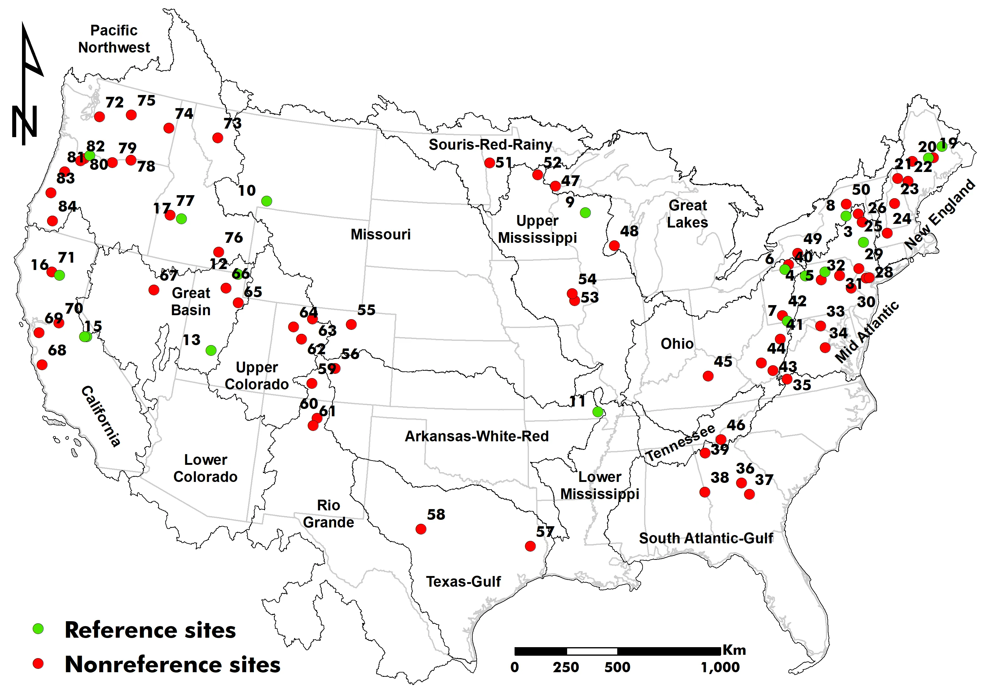
From an initial pool of 9067 USGS gaging stations, 18 reference sites and 66 non-reference sites with complete peak flow records longer than 100 years were selected. For every gage selected in this study, we retrieved the annual maximum discharge series (one peak value per water year) from the USGS National Water Information System (NWIS) and used that series in all subsequent analyses. By contrasting reference gages, where long-term changes are attributed chiefly to climate variability [
31,
32], with non-reference gages that are additionally affected by urbanization, dam regulation, and other basin alterations [
17,
18], we can separate the climate-driven component of nonstationarity in flood frequency from the combined climate-plus-anthropogenic signal. The spatial distribution of the study sites is presented in , and other geographical details are provided in the Supporting Information section (Table S1).
. Spatial distribution of the 18 reference (green circles) and 66 non-reference (red circles) gaging stations in the conterminous United States. The numbers correspond to the Object IDs in supplementary Table S1. Water resources regions (gray lines) correspond to Level-02 hydrologic units (HUC02) delineated by the USGS.
4. Results and Discussion
4.1. LP3 Performance
To evaluate how well the LP3 distribution estimates moderate flood quantiles, we computed the ratio (R) of the observed quantile (Obs) to its LP3 estimate (Est). A ratio greater than one (R = Obs/Est > 1) indicates that LP3 underestimates the quantile, whereas a ratio below one (R = Obs/Est < 1) indicates overestimation. The cross-correlation values for the goodness-of-fit test [
44] ranged from 0.68 to 0.98 across both reference and non-reference sites, suggesting that LP3 provides a reasonable statistical fit to peak flow observations nationwide [
50].
We treated sites as follows to maintain sufficient record for reliable quantile estimation. Where a statistically significant change point was detected, R values were calculated for floods with the return periods of 2 to 25 years using the pre-change, post-change, and entire record segments. For sites without a statistically significant change point, the analysis used the whole record and covered floods with 2 to 100 years return periods.
4.2. Statistically Significant Change Point
37 of the 84 sites exhibited a statistically significant change point (
p-value ≤ 0.05). Of these, four were reference sites (out of 18) and 33 were non-reference sites (out of 66) ().
.
Ratio (R) of observed peak flows to the corresponding LP3 flood quantile estimate (Obs/Est) for reference sites (4 out of 18) and non-reference sites (33 out of 66) with statistically significant change points.
Period
of Analysis |
Study
Site |
Return Period (T, Years) |
| T = 2 |
T = 5 |
T = 10 |
T = 25 |
| R < 1 (R > 1) a,b |
R < 1 (R > 1) |
R < 1 (R > 1) |
R < 1 (R > 1) |
| Pre change point |
Reference |
2/4 (50%) |
1/4 (75%) |
2/4 (50%) |
0/4 (100%) |
| Non-reference |
13/33 (61%) |
18/33 (45%) |
20/33 (39%) |
0/33 (100%) |
| Total sites |
15/37 (59%) |
19/37 (49%) |
22/37 (41%) |
0/37 (100%) |
| Post change point |
Reference |
1/4 (75%) |
2/4 (50%) |
2/4 (50%) |
3/4 (25%) |
| Non-reference |
12/33 (64%) |
11/33 (67%) |
16/33 (52%) |
22/33 (33%) |
| Total sites |
13/37 (65%) |
13/37 (65%) |
18/37 (51%) |
25/37 (32%) |
| Entire record |
Reference |
3/4 (75%) |
2/4 (50%) |
4/4 (0%) |
2/4 (50%) |
| Non-reference |
13/33 (61%) |
20/33 (39%) |
20/33 (39%) |
18/33 (45%) |
| Total sites |
16/37 (57%) |
22/37 (41%) |
24/37 (35%) |
20/37 (46%) |
As an example, at USGS gage 03082500 (Youghiogheny River at Connellsville, Pennsylvania) the Pettitt test identifies a break in 1942, the year Youghiogheny River Lake dam was completed 29 miles upstream, supplementing flow regulation already imposed by Deep Creek Reservoir since 1925. This case confirms that some breakpoints correspond to clear physical drivers such as dam construction or river regulation. We emphasize, however, that not every shift can be tied to a single documented cause. Several factors, such as gradual climatic trends, minor impoundments, or evolving water use, often also interact. A full attribution would require site-specific hydrologic modeling, which is beyond this study’s scope, but the provided example demonstrates the practical aspect of the segmentation approach.
4.3. Two-Year Flood
Because segmentation shortens each record, we restrict our frequency curves to return periods equal to or less than 25 years. Estimates for rarer events could be developed with (i) peak-over-threshold or partial duration series, (ii) regional pooling, or (iii) nonstationary models with time-varying distribution parameters. A full evaluation of these approaches is deferred to future work.
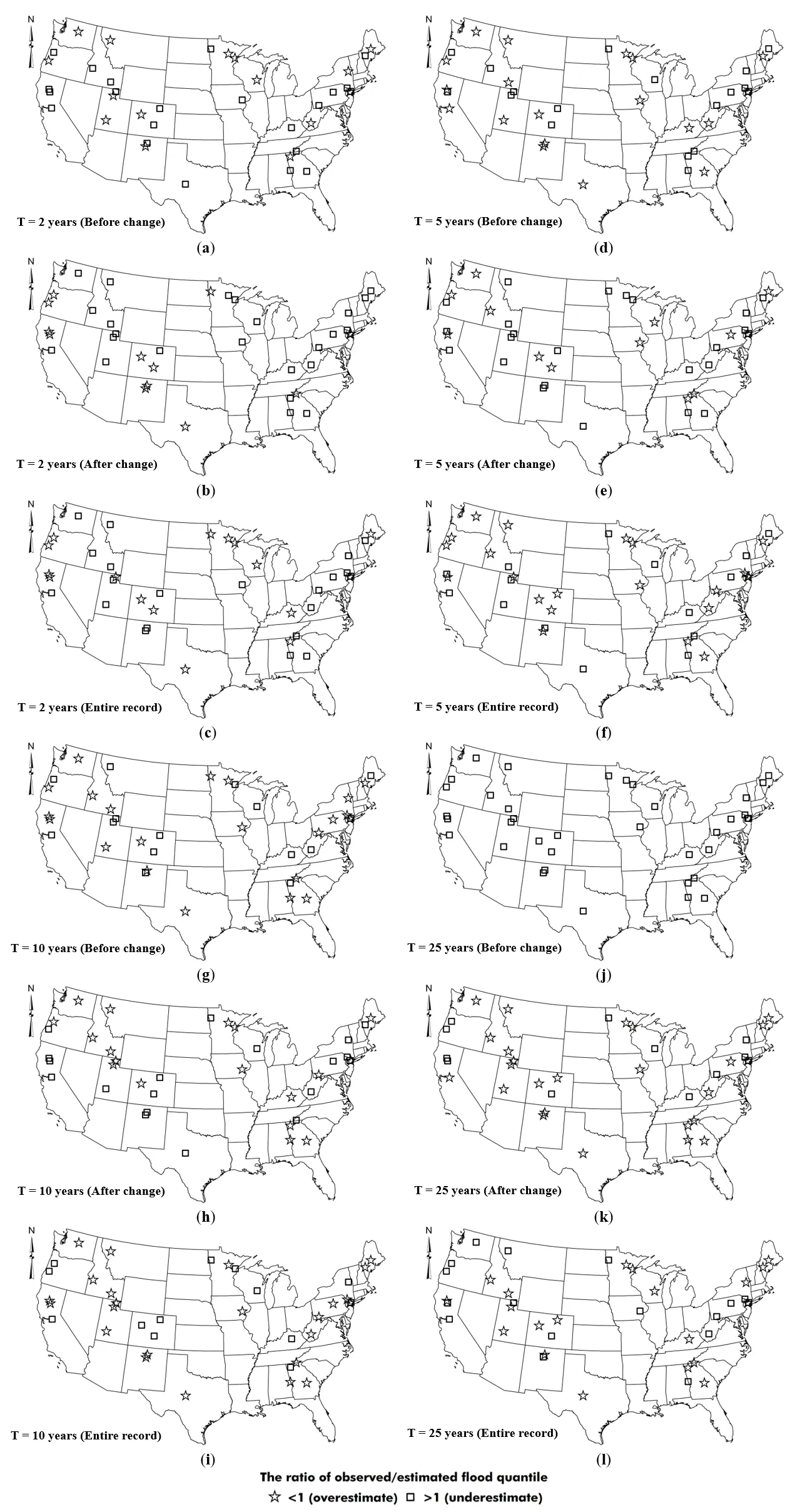
For a return period of two years, LP3 performed well (R < 1) at 41% (15 out of 37) of the study sites before the regime shift in peak flow records (a; ). At the remaining sites, LP3 underestimated the flood quantiles. No clear spatial pattern emerged in the locations where LP3 under- or over-estimated the flood quantile. After the change point (b), LP3 overestimated the 2-year flood at 35% (13 out of 37) of the sites. LP3 tended to underestimate floods across much of the eastern United States but performed reasonably in the central and western regions.
Flood quantile estimates for the entire period of record were consistent with the post change point results (c). This outcome suggests that larger floods occurring after the change point influenced the distribution fitted to the full record.
. Ratio (R) of observed to LP3-estimated flood quantiles with return periods of 2 (<b>a</b>–<b>c</b>), 5 (<b>d</b>–<b>f</b>), 10 (<b>g</b>–<b>i</b>), and 25 (<b>j</b>–<b>l</b>) years for the periods before the change point, after the change point, and the entire record. All change points are statistically significant (<i>p</i>-value ≤ 0.05).
d–f presents the results for floods with a 5-year return period before the change point, after the change point, and for the entire record, respectively. Overall, LP3 overestimated the flood quantiles at a slight majority of sites (51%; ). LP3 performance was generally unreliable along much of the East Coast. After the change point (e), LP3 produced reliable estimates at 35% of the study sites, with no distinct spatial pattern in where it performed well or poorly. When the entire record was analyzed (f), the estimated quantiles exceeded the observed peak flows at 22 of the 37 sites (59%). Notably, LP3 yielded reliable estimates in the Pacific Northwest.
4.5. Ten-Year Flood
Before the change point, LP3 overestimated the 10-year flood at 59% of the study sites, most of which are on the East Coast (g; ). After the change point, the distribution overestimated flood quantiles for almost half of the sites; its predictions were reliable in the Pacific Northwest but unreliable in California (h). When the entire record was used, LP3 produced better estimates for 65% of the sites, mostly located along the East Coast and in the Great Basin (i).
4.6. Twenty Five-Year Flood
The most compelling pattern emerged for the 25-year flood estimates when only the period before the change point was considered (j; ). At all 37 sites with a statistically significant change point, the observed-to-estimated ratio exceeded one, indicating that LP3 consistently underestimated the 25-year flood. When only the post-change record was utilized, LP3 overestimated floods at 68% of the sites (k), although estimates were reliable in the South Atlantic Gulf, Great Basin, and Rio Grande regions. Using the entire record, LP3 returned satisfactory estimates at 20 of 37 sites (54%) (l), tending to overestimate floods in New England and underestimate them in the Mid-Atlantic and along much of the West Coast.
As the return period increased, analyses based on the post-change record generally yielded better quantile estimates, especially for 10-year floods and beyond. Our result aligns with earlier work showing nationwide increases in the frequency, magnitude, and duration of high-percentile floods, driven mainly by climatic variability [
20,
26,
27,
28,
51,
52,
53].
Climate variations and anthropogenic disturbances, such as land use change or river regulation, can also shift the timing of floods. In the northeastern United States, annual maximum floods historically peaked in spring [
54]. Warmer winters now trigger earlier snowmelt and, when combined with rainfall [
55], lead to earlier flood occurrence or shift in timing [
10,
56]. Summer precipitation has increased in the Northeast too [
57,
58,
59], creating the potential for peak flows comparable to spring events [
10].
In the central United States, the timing of high quantile precipitation has shifted from summer to spring [
60]. When accompanied by lower evapotranspiration and moist soil, it promotes overland flow, producing larger spring floods. These shifts from rain-on-snow floods to rainfall-driven events generate a new population of flood events that differs from historical records. Consequently, post-change flood data may better represent current flood behavior in a region of interest. However, when the highest historical peaks fall in the pre-change record or when paleoflood information is added, deciding whether the pre-, post-, or full record provides the most reliable quantile estimates becomes more complex.
4.7. Statistically Insignificant Change Point
For the 47 study sites where the change point was not statistically significant (
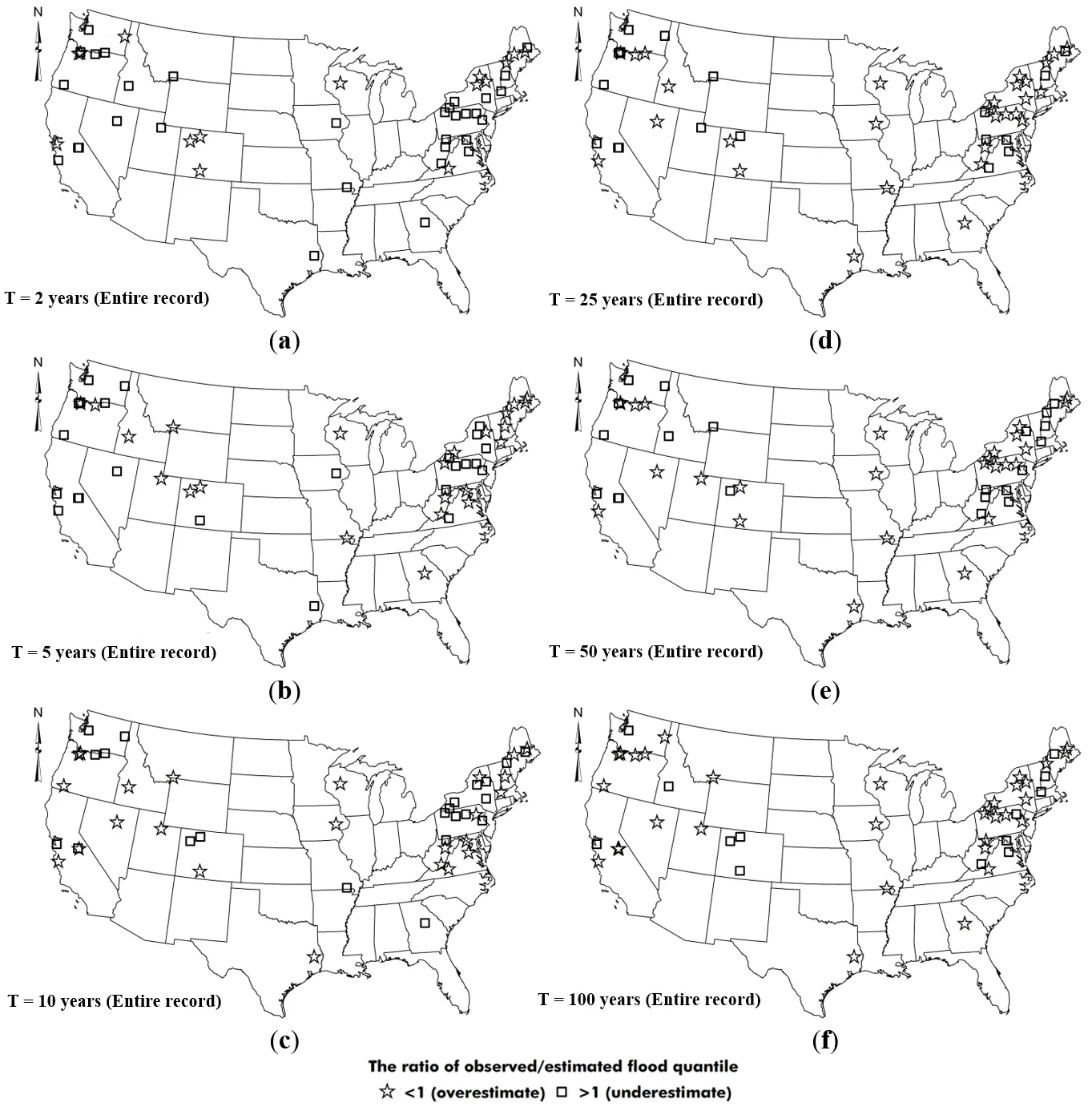
p-value > 0.05), we compared observed and estimated flood quantiles with return periods of 2–100 years over the entire record. LP3 did not reliably estimate the 2-year flood at 68% of these sites, most of which are in New England and the Mid-Atlantic (; a). LP3 underestimated the 5-year flood at 51% of the study sites, largely in California and the Mid-Atlantic (b). LP3 overestimated the 5-year flood at 49% of the study sites, largely in New England (b). For the 10-year flood, LP3 performed well at 53% of the sites, mainly in New England, the Upper Mississippi, and the Great Basin (c).
At the 25-year return period, LP3 overestimated flood quantiles for 62% of the sites, mainly in New England and the Mid-Atlantic (d). When the return period increased to 50 years, LP3 performed reliably at 55% of sites, mostly in the Upper Colorado, Upper Mississippi, and Lower Mississippi regions (e). For the 100-year flood, LP3 provided reliable estimates at 34 out of 47 sites (72%), located in the Pacific Northwest, California, the Great Basin, Upper Colorado, Upper Mississippi, and the Mid-Atlantic (f).
.
Same as , but for sites with statistically insignificant change points.
Study
Site |
Return Period (T, Years) |
| T = 2 |
T = 5 |
T = 10 |
T = 25 |
T = 50 |
T = 100 |
| R < 1 (R > 1) a,b |
R < 1 (R > 1) |
R < 1 (R > 1) |
R < 1 (R > 1) |
R < 1 (R > 1) |
R < 1 (R > 1) |
| Reference |
3/14 (79%) |
7/14 (50%) |
6/14 (57%) |
9/14 (36%) |
9/14 (36%) |
13/14 (7%) |
| Non-reference |
12/33 (64%) |
16/33 (52%) |
19/33 (42%) |
20/33 (39%) |
17/33 (48%) |
21/33 (36%) |
| Total sites |
15/47 (68%) |
23/47 (51%) |
25/47 (47%) |
29/47 (38%) |
26/47 (45%) |
34/47 (28%) |
. Ratio (R) of observed to LP3-estimated flood quantiles based on the entire flood record at sites where the change point was not statistically significant (<i>p</i>-value > 0.05) for floods with return periods of (<b>a</b>) 2 years; (<b>b</b>) 5 years; (<b>c</b>) 10 years; (<b>d</b>) 25 years; (<b>e</b>) 50 years; and (<b>f</b>) 100 years.
Numerous studies have focused on improving flood quantile estimates to help reduce property damage, crop loss, and fatalities [
35]. Nonstationarity in the data structure could degrade these estimates [
24,
61,
62,
63]. Detecting a change point in peak flow times series offers a simple way to mitigate nonstationarity: analyzing the flood records separately before and after the change point may yield more reliable quantiles than treating the entire record as one homogeneous data sample.
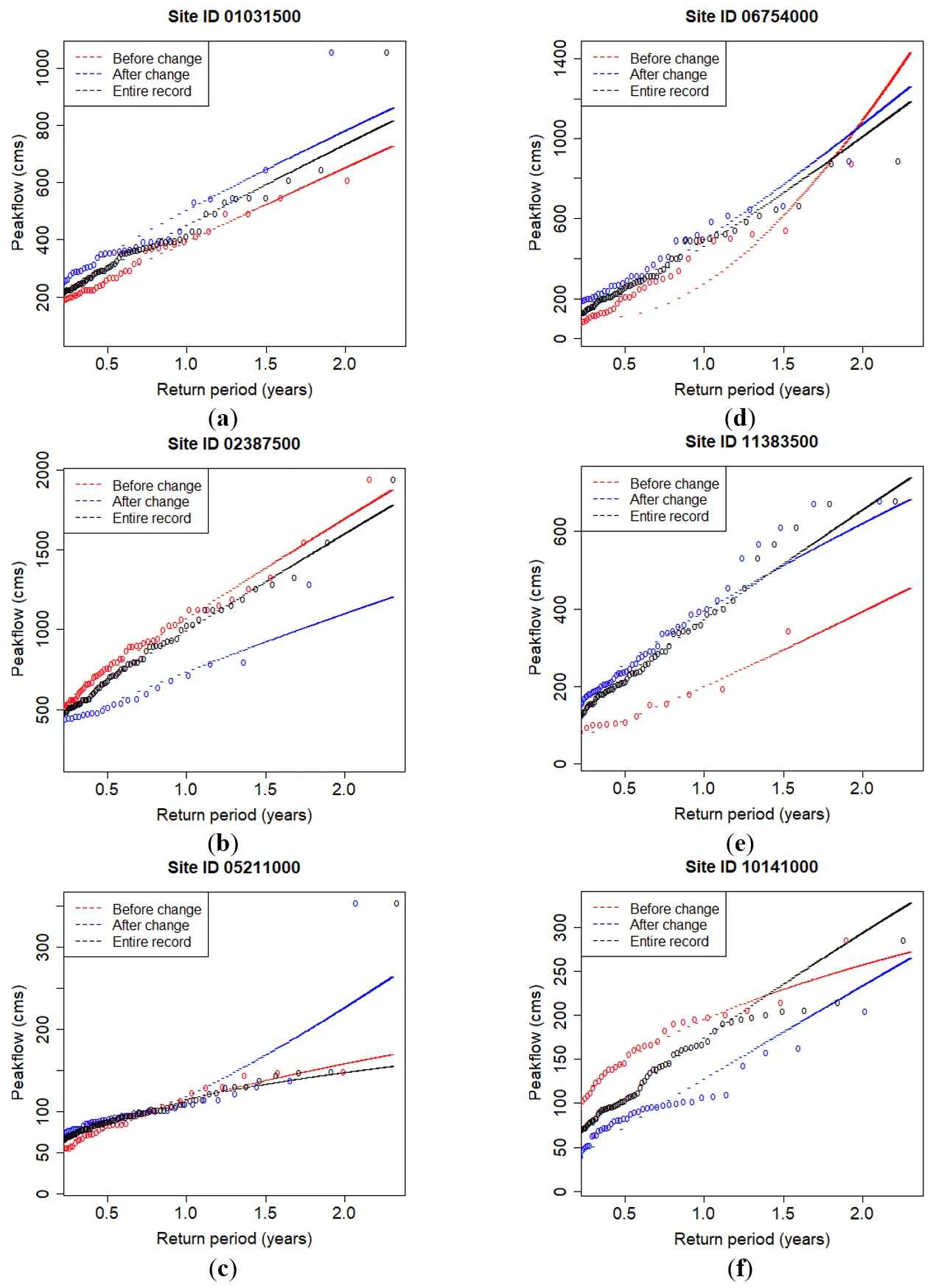
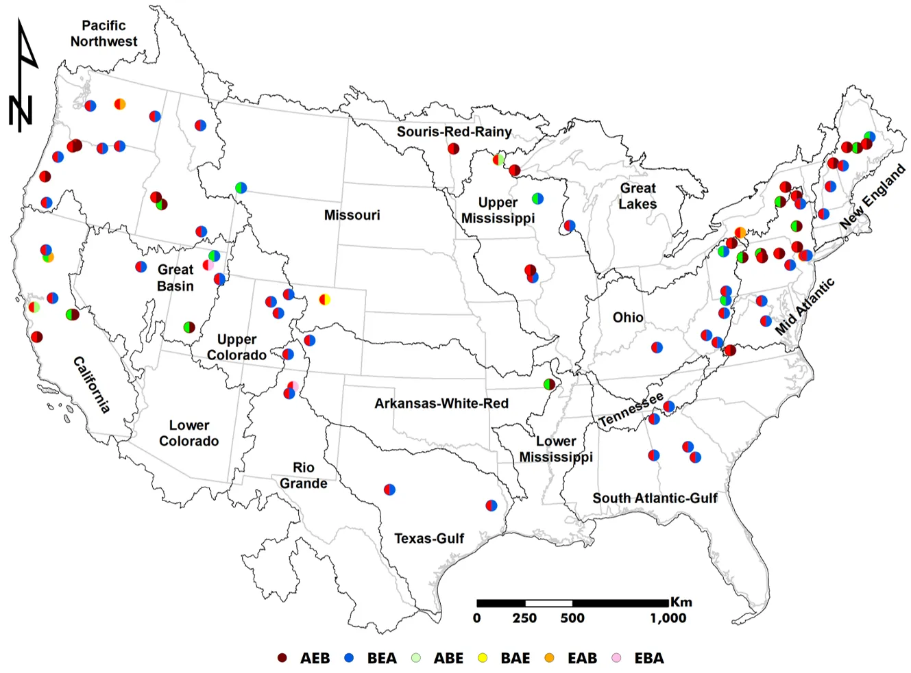
We therefore generated flood frequency curves for 18 reference and 66 non-reference sites, dividing each site's peak flow record into pre-change and post-change periods. We intended to determine whether parsing the flood information into two independent periods can improve quantile estimates. Depending on whether the historical peak occurs in the pre- or post-change segment, the three curves of before (B), after (A), and entire record (E) can likely follow one of the schematic patterns shown in a–f.
In the Pacific Northwest, California, the Souris-Red-Rainy basin, northern Mid-Atlantic, and northern New England, the post-change curve produced the highest quantile estimates, exceeding both the entire-record and pre-change curves (scenario AEB, ). Conversely, in areas west of the Colorado, north of the Rio Grande, west of Arkansas, the Texas Gulf, Tennessee, the South Atlantic–Gulf, Ohio, the coastal Mid-Atlantic, and central New England, the pre-change curve returned the largest estimates, surpassing both the entire record and the post-change segment (scenario BEA, ).
In general, most reference sites followed the AEB pattern, suggesting that recent climate-driven nonstationarity has detectable influence on their flood quantiles (a and ). On the other hand, many non-reference sites displayed the BEA pattern, which may be due to dominant anthropogenic disturbances such as dam construction or river regulation. As such, the pre-change flood record at non-reference sites still produces the highest quantiles despite recent climatic variability (b and ).
For gage 01031500, the Pettitt test identified a significant change point in 1967. Applying the LP3 distribution to the 1903–2015 record yields a 100-year flood estimate of approximately 620 m
3/s. Segmenting the record results in Q
100 estimates of about 550 m
3/s before the change and 780 m
3/s after. These pre- and post-change estimates form a practical uncertainty band around the entire record value, illustrating how a simple segmentation approach can highlight the potential for under- or over-design when nonstationarity exists.
. Flood frequency curves analysis for selected sites where parsing the record into pre- and post-change periods retuned different results from those obtained with the entire record. The x-axis is the base-10 logarithm of return period in years (2.0 means 100 or 10<sup>2</sup>); the y-axis is peak flow in cubic meters per second (m<sup>3</sup>/s or cms). Six distinct patterns are observed: (<b>a</b>) After–Entire–Before (AEB), where the estimated quantiles decline from the post-change period, to the entire record, to the pre-change period; (<b>b</b>) Before–Entire–After (BEA), where the estimated quantiles decline from the pre-change period, to the entire record, to the post-change period; (<b>c</b>) After–Before–Entire (ABE), where the estimated quantiles decline from the post-change period, to the pre-change period, to the entire record; (<b>d</b>) Before–After–Entire (BAE), where estimated quantiles decline from the pre-change period, to the post-change period, to the entire record; (<b>e</b>) Entire–After–Before (EAB), where the estimated quantiles decline from the entire record, to the post-change period, to the pre-change period; and (<b>f</b>) Entire–Before–After (EBA), where the estimated quantiles decline from the entire record, to the pre-change period, to the post-change period.
. Spatial distribution of the flood frequency analysis results when the record is parsed into periods before and after the change point and compared with the entire record. The left half-circle at each site is green for reference gages and red for non-reference gages. The right half-circle indicates a scenario according to a–f: (a) After–Entire–Before (AEB); (b) Before–Entire–After (BEA); (c) After–Before–Entire (ABE); (d) Before–After–Entire (BAE); (e) Entire–After–Before (EAB); and (f) Entire–Before–After (EBA).
5. Conclusions and Summary
We examined annual maximum flood series from 18 reference and 66 non-reference USGS sites, each with more than 100 years of records. Comparing the flood quantiles for reference and non-reference sites helped us to explore the effects of climate-driven nonstationarity on frequency analysis separately from the combined effects of climate variability and anthropogenic disturbances. We utilized the nonparametric Pettitt test to detect a single shift in each gage flood record. Where the shift was statistically significant (
p-value ≤ 0.05), the flood record was divided into “before” and “after” segments for independent flood frequency analysis.
Flood frequency curves were fitted with the LP3 distribution, using the product moment formulation of [
46]. The peak flow record length varied substantially among study sites before and after the change point. Because the lengths of the pre- and post-change records varied widely among sites, the study focused on return periods up to 25 years. Longer flood time series created by peaks-over-threshold or partial series approach could extend the analysis to rarer events and clarify whether high-quantile floods (>25 years) have intensified in recent decades. Should such increases be confirmed, the conventional LP3 model fitted to post-change data is likely to remain adequate; however, although the Pettitt split mitigates the most prominent shift, we do not claim that each segment is perfectly stationary. Instead, the segmented LP3 curve should be viewed as one line of evidence, to be considered alongside nonstationary models when critical design decisions hinge on upper-tail quantiles.
At most reference sites, analyzing only the post-change segment produced the largest quantile estimates, underscoring the influence of recent climate-driven nonstationarity. Many non-reference sites, however, showed higher quantile estimates in the pre-change segment, highlighting long-standing regulation, land-use change, or other human alterations. Apparent regional patterns, such as closer LP3 fits in the South Atlantic-Gulf region and systematic overestimation in New England, should be considered preliminary. With a limited number of century-length gages per water resources region (HUC02), our sample is too limited for a rigorous regional or hierarchical analysis. Expanding the dataset to include additional, but shorter records, would enable a formal clustering or Bayesian hierarchical framework that may reveal spatially coherent deviations from the segmented LP3 model.
These contrasting patterns underscore that a statistical distribution may not always need to be fitted to the entire period of record; instead, it may be applied to a segment that minimizes nonstationarity (regardless of its source) while yielding reasonable quantile estimates. Updated quantile estimates can help watershed managers prepare for shifts in flood magnitude and frequency under nonstationary conditions.
Supplementary Materials
The following supporting information can be found at: https://www.sciepublish.com/article/pii/623, Table S1: The description of 18 reference and 66 nonreference study sites with more than 100 years of peak flow data across the contiguous United States.
Acknowledgments
Authors would like to acknowledge and extend their gratitude for the support provided by Kansas State University for the current research. The work was conducted between 2018–2019, during Berton’s tenure as a postdoctoral fellow and Rahmani’s tenure as an assistant professor in the Department of Biological and Agricultural Engineering at Kansas State University.
Author Contributions
R.B.: Conceptualization, Methodology, Software, Validation, Formal Analysis, Investigation, Data Curation, Writing—Original Draft Preparation, Writing–Review & Editing, Visualization; V.R.: Conceptualization, Validation, Resources, Writing—Review & Editing, Supervision, Project Administration, Funding Acquisition.
Ethics Statement
Not applicable.
Informed Consent Statement
Not applicable.
Data Availability Statement
The data presented in this study are available on request from the corresponding authors.
Funding
This research was funded by the Department of Biological and Agricultural Engineering at Kansas State University through the contribution number of “19-102-J” of the Kansas Agricultural Experiment Station.
Declaration of Competing Interes
The authors declare that they have no known competing financial interests or personal relationships that could have appeared to influence the work reported in this paper. Additionally, the views expressed in this paper are those of the authors and do not necessarily reflect the official positions or opinions of their affiliated institutions.
References
-
1.
Donat MG, Lowry AL, Alexander LV, O’Gorman PA, Maher N. More extreme precipitation in the world’s dry and wet regions.
Nat. Clim. Chang. 2016,
6, 508–513. doi:10.1038/nclimate2941.
[Google Scholar]
-
2.
Douville H, Raghavan K, Renwick J, Allan RP, Arias PA, Barlow M, et al. IPCC AR6: Water Cycle Changes. In Climate Change 2021: The Physical Science Basis. Contribution of Working Group I to the Sixth Assessment Report of the Intergovernmental Panel on Climate Change; Masson-Delmotte V, Zhai P, Pirani A, Connors SL, Péan C, Berger S, Eds.; Cambridge University Press: Cambridge, UK; New York, NY, USA, 2021, pp. 1055–1210. doi:10.1017/9781009157896.010
-
3.
Hoerling M, Eischeid J, Perlwitz J, Quan XW, Wolter K, Cheng L. Characterizing Recent Trends in U.S. Heavy Precipitation.
J. Clim. 2016,
29, 2313–2332. doi:10.1175/JCLI-D-15-0441.1.
[Google Scholar]
-
4.
Ingram W. Extreme precipitation: Increases all round.
Nat. Clim. Chang. 2016,
6, 443–444.
[Google Scholar]
-
5.
Fowler HJ, Blenkinsop S, Green A, Davies PA. Precipitation extremes in 2023.
Nat. Rev. Earth Environ. 2024,
5, 250–252. doi:10.1038/s43017-024-00547-9.
[Google Scholar]
-
6.
Myhre G, Alterskjær K, Stjern CW, Hodnebrog Ø, Marelle L, Samset BH, et al. Frequency of extreme precipitation increases extensively with event rareness under global warming.
Sci. Rep. 2019,
9, 16063. doi:10.1038/s41598-019-52277-4.
[Google Scholar]
-
7.
Westra S, Fowler HJ, Evans JP, Alexander LV, Berg P, Johnson F, et al. Future changes to the intensity and frequency of short-duration extreme rainfall.
Rev. Geophys. 2014,
52, 522–555. doi:10.1002/2014RG000464.
[Google Scholar]
-
8.
Bertola M, Viglione A, Vorogushyn S, Lun D, Merz B, Blöschl G. Do small and large floods have the same drivers of change? A regional attribution analysis in Europe. Hydrol.
Earth Syst. Sci. 2021,
25, 1347–1364. doi:10.5194/hess-25-1347-2021.
[Google Scholar]
-
9.
Archfield SA, Hirsch RM, Viglione A, Blöschl G. Fragmented patterns of flood change across the United States.
Geophys. Res. Lett. 2016,
43, 10232–10239. doi:10.1002/2016GL070590.
[Google Scholar]
-
10.
Berton R, Driscoll CT, Chandler DG. Changing climate increases discharge and attenuates its seasonal distribution in the northeastern United States.
J. Hydrol. Reg. Stud. 2016,
5, 164–178. doi:10.1016/j.ejrh.2015.12.057.
[Google Scholar]
-
11.
Hallegatte S, Green C, Nicholls RJ, Corfee-Morlot J. Future flood losses in major coastal cities.
Nat. Clim. Chang. 2013,
3, 802–806. doi:10.1038/nclimate1979.
[Google Scholar]
-
12.
Ivancic TJ, Shaw SB. Examining why trends in very heavy precipitation should not be mistaken for trends in very high river discharge.
Clim. Chang. 2015,
133, 681–693. doi:10.1007/s10584-015-1476-1.
[Google Scholar]
-
13.
Saharia M, Kirstetter P-E, Vergara H, Gourley JJ, Hong Y. Characterization of floods in the United States.
J. Hydrol. 2017,
548, 524–535. doi:10.1016/j.jhydrol.2017.03.010.
[Google Scholar]
-
14.
Schedel JR, Schedel AL. Analysis of Variance of Flood Events on the U.S. East Coast: The Impact of Sea-Level Rise on Flood Event Severity and Frequency.
J. Coast. Res. 2018,
341, 50–57. doi:10.2112/JCOASTRES-D-16-00205.1.
[Google Scholar]
-
15.
Ward PJ, Jongman B, Aerts JCJH, Bates PD, Botzen WJW, Diaz Loaiza A, et al. A global framework for future costs and benefits of river-flood protection in urban areas.
Nat. Clim. Chang. 2017,
7, 642–646. doi:10.1038/nclimate3350.
[Google Scholar]
-
16.
Zahmatkesh Z, Karamouz M. An uncertainty-based framework to quantifying climate change impacts on coastal flood vulnerability: case study of New York City.
Environ. Monit. Assess. 2017,
11, 567. doi:10.1007/s10661-017-6282-y.
[Google Scholar]
-
17.
Burn DH, Whitfield PH. Changes in cold region flood regimes inferred from long-record reference gauging stations.
Water Resour. Res. 2017,
53, 2643–2658. doi:10.1002/2016WR020108.
[Google Scholar]
-
18.
Rice JS, Emanuel RE, Vose JM, Nelson SAC. Continental U.S. streamflow trends from 1940 to 2009 and their relationships with watershed spatial characteristics.
Water Resour. Res. 2015,
51, 6262–6275. doi:10.1002/2014WR016367.
[Google Scholar]
-
19.
Schroeder AJ, Gourley JJ, Hardy J, Henderson JJ, Parhi P, Rahmani V, et al. The development of a flash flood severity index.
J. Hydrol. 2016,
541, 523–532. doi:10.1016/j.jhydrol.2016.04.005.
[Google Scholar]
-
20.
Najibi N, Devineni N. Recent trends in the frequency and duration of global floods.
Earth Syst. Dyn. 2018,
9, 757–783. doi:10.5194/esd-9-757-2018.
[Google Scholar]
-
21.
Barth NA, Villarini G, Nayak MA, White K. Mixed populations and annual flood frequency estimates in the western United States: The role of atmospheric rivers.
Water Resour. Res. 2017,
53, 257–269. doi:10.1002/2016WR019064.
[Google Scholar]
-
22.
Collins MJ. Evidence for changing flood risk in New England since the late 20th century.
J. Am. Water Resour. Assoc. 2009,
45, 279–290.
[Google Scholar]
-
23.
Mallakpour I, Villarini G. The changing nature of flooding across the central United States.
Nat. Clim. Chang. 2015,
5, 250–254. doi:10.1038/nclimate2516.
[Google Scholar]
-
24.
Maurer EP, Kayser G, Doyle L, Wood AW. Adjusting Flood Peak Frequency Changes to Account for Climate Change Impacts in the Western United States.
J. Water Resour. Plan. Manag. 2018,
144, 05017025. doi:10.1061/(ASCE)WR.1943-5452.0000903.
[Google Scholar]
-
25.
Villarini G, Smith JA. Flood peak distributions for the eastern United States.
Water Resour. Res. 2010,
46, W06504. doi:10.1029/2009WR008395.
[Google Scholar]
-
26.
Kundzewicz ZW, Kanae S, Seneviratne SI, Handmer J, Nicholls N, Peduzzi P, et al. Flood risk and climate change: global and regional perspectives.
Hydrol. Sci. J. 2014,
59, 1–28. doi:10.1080/02626667.2013.857411.
[Google Scholar]
-
27.
Luke A, Vrugt JA, AghaKouchak A, Matthew R, Sanders BF. Predicting nonstationary flood frequencies: Evidence supports an updated stationarity thesis in the United States.
Water Resour. Res. 2017,
53, 5469–5494. doi:10.1002/2016WR019676.
[Google Scholar]
-
28.
Slater LJ, Villarini G. Recent trends in U.S. flood risk.
Geophys. Res. Lett. 2016,
43, 12,428-12,436. doi:10.1002/2016GL071199.
[Google Scholar]
-
29.
Villarini G, Smith JA, Baeck ML, Krajewski WF. Examining Flood Frequency Distributions in the Midwest U.S.
J. Am. Water Resour. Assoc. 2011,
47, 447–463. doi:10.1111/j.1752-1688.2011.00540.x.
[Google Scholar]
-
30.
Lins HF, Slack JR. Seasonal and regional characteristics of US streamflow trends in the United States from 1940 to 1999.
Phys. Geogr. 2005,
26, 489–501.
[Google Scholar]
-
31.
Falcone J. GAGES-II: Geospatial Attributes of Gages for Evaluating Streamflow (Vector Digital Data); U.S. Geological Survey: Reston, VA, USA, 2011.
-
32.
Lins HF. USGS Hydro-Climatic Data Network 2009 (HCDN–2009) (Fact Sheet); U. S. Geological Survey: Reston, VA, USA, 2012.
-
33.
Pettitt AN. A Non-Parametric Approach to the Change-Point Problem.
J. R. Stat. Soc. Ser. C Appl. Stat. 1979,
28, 126–135.
[Google Scholar]
-
34.
Conte LC, Bayer DM, Bayer FM. Bootstrap Pettitt test for detecting change points in hydroclimatological data: case study of Itaipu Hydroelectric Plant, Brazil.
Hydrol. Sci. J. 2019,
64, 1312–1326. doi:10.1080/02626667.2019.1632461.
[Google Scholar]
-
35.
England JF, Jr., Cohn TA, Faber BA, Stedinger JR, Thomas WO, Jr., Veilleux AG, et al. Guidelines for Determining Flood Flow Frequency—Bulletin 17C (Report No. 4-B5), Techniques and Methods; U.S. Geological Survey: Reston, VA, USA, 2018. doi:10.3133/tm4B5.
-
36.
Rodionov SN. A sequential algorithm for testing climate regime shifts.
Geophys. Res. Lett. 2004,
31, 4. doi:10.1029/2004GL019448.
[Google Scholar]
-
37.
Xin Y, Stedinger JR. LP3 Flood Frequency Analysis Including Climate Change. In Proceedings of World Environmental and Water Resources Congress 2018, Minneapolis, MN, USA, 3–7 June 2018; pp. 459–467. doi:10.1061/9780784481400.043.
-
38.
Kjeldsen TR, Jones DA. A formal statistical model for pooled analysis of extreme floods.
Hydrol. Res. 2009,
40, 465–480. doi:10.2166/nh.2009.055.
[Google Scholar]
-
39.
Rahmani V, Hutchinson S.L, Harrington Jr JA, Hutchinson JMS, Anandhi A. Analysis of temporal and spatial distribution and change-points for annual precipitation in Kansas, USA.
Int. J. Climatol. 2015,
35, 3879–3887. doi:10.1002/joc.4252.
[Google Scholar]
-
40.
Pohlert T. Non-Parametric Trend Tests and Change-Point Detection. R package version 1.1.0. 2018. Available online: https://cran.r-project.org/web/packages/trend/vignettes/trend.pdf (accessed on 29 July 2025)
-
41.
Stedinger JR. Flood frequency analysis. In Handbook of Applied Hydrology, Singh VP, Ed.; McGraw Hill Book Co.: New York, NY, USA, 2016.
-
42.
Karim MA, Chowdhury JU. A comparison of four distributions used in flood frequency analysis in Bangladesh.
Hydrol. Sci. J. 1995,
40, 55–66. doi:10.1080/02626669509491390.
[Google Scholar]
-
43.
Lamontagne JR, Stedinger JR. Examination of the Spencer-McCuen Outlier-Detection Test for Log-Pearson Type 3 Distributed Data.
J. Hydrol. Eng. 2016,
21, 04015069. doi:10.1061/(ASCE)HE.1943-5584.0001321.
[Google Scholar]
-
44.
Serago JM, Vogel RM. Parsimonious nonstationary flood frequency analysis.
Adv. Water Resour. 2018,
112, 1–16. doi:10.1016/j.advwatres.2017.11.026.
[Google Scholar]
-
45.
Vogel RM, Kroll CN. Low‐Flow Frequency Analysis Using Probability‐Plot Correlation Coefficients.
J. Water Resour. Plan. Manag. 1989,
115, 338–357. doi:10.1061/(ASCE)0733-9496(1989)115:3(338).
[Google Scholar]
-
46.
Stedinger JR, Vogel RM, Foufoula-Georgiou E. Frequency analysis of extreme events. In Handbook of Hydrology; Maidment DR, Ed.; McGraw-Hill: New York, NY, USA, 1993; p. 1424.
-
47.
Bobée B. The Log Pearson type 3 distribution and its application in hydrology.
Water Resour. Res. 1975,
11, 681–689. doi:10.1029/WR011i005p00681.
[Google Scholar]
-
48.
Derenzo SE. Approximations for Hand Calculators Using Small Integer Coefficients.
Math. Comput. 1977,
31, 214–222. doi:10.2307/2005791.
[Google Scholar]
-
49.
R Core Team. R: A Language and Environment for Statistical Computing. 2018. Available online: https://www.r-project.org/ (accessed on 29 July 2025).
-
50.
Izinyon O, Ehiorobo J. L-moments approach for flood frequency analysis of river Okhuwan in Benin-Owena River basin in Nigeria.
Niger. J. Technol. 2014,
33, 10. doi:10.4314/njt.v33i1.2.
[Google Scholar]
-
51.
Mei X, Dai Z, Tang Z, van Gelder PHAJM. Impacts of historical records on extreme flood variations over the conterminous United States.
J. Flood Risk Manag. 2018,
11, S359–S369. doi:10.1111/jfr3.12223.
[Google Scholar]
-
52.
Read LK, Vogel RM. Reliability, return periods, and risk under nonstationarity.
Water Resour. Res. 2015,
51, 6381–6398. doi:10.1002/2015WR017089.
[Google Scholar]
-
53.
Villarini G, Serinaldi F, Smith JA, Krajewski WF. On the stationarity of annual flood peaks in the continental United States during the 20th century.
Water Resour. Res. 2009,
45, 1–17. doi:10.1029/2008WR007645.
[Google Scholar]
-
54.
Baldwin HL, McGuinness CL. A Primer on Ground Water (Report), General Interest Publication; Geological Survey: Washington, DC, USA, 1963.
-
55.
Huntington TG, Hodgkins GA, Keim BD, Dudley RW. Changes in the proportion of precipitation occurring as snow in New England (1949–2000).
J. Clim. 2004,
17, 2626–2636. doi:10.1175/1520-0442(2004)017<2626:CITPOP>2.0.CO;2.
[Google Scholar]
-
56.
Frumhoff PC, McCarthy JJ, Melillo JM, Moser SC, Wuebbles DJ. Confronting Climate Change in the U.S. Northeast: Science, Impacts, and Solutions. Synthesis Report of the Northeast Climate Impacts Assessment (NECIA); Union of Concerned Scientists (UCS): Cambridge, MA, USA, 2007.
-
57.
Campbell JL, Driscoll CT, Pourmokhtarian A, Hayhoe K. Streamflow responses to past and projected future changes in climate at the Hubbard Brook Experimental Forest, New Hampshire, United States.
Water Resour. Res. 2011,
47, 15. doi:10.1029/2010WR009438.
[Google Scholar]
-
58.
Hayhoe K, Wake CP, Huntington TG, Luo L, Schwartz M.D, Sheffield J, et al. Past and future changes in climate and hydrological indicators in the US Northeast.
Clim. Dyn. 2007,
28, 381–407. doi:10.1007/s00382-006-0187-8.
[Google Scholar]
-
59.
Huntington TG, Billmire M. Trends in Precipitation, Runoff, and Evapotranspiration for Rivers Draining to the Gulf of Maine in the United States*.
J. Hydrometeorol. 2014,
15, 726–743. doi:10.1175/JHM-D-13-018.1.
[Google Scholar]
-
60.
Rahmani V, Hutchinson SL, Harrington JA, Hutchinson JMS. Analysis of frequency and magnitude of extreme rainfall events with potential impacts on flooding: a case study from the central United States: Extreme rainfall events with potential impacts on flooding.
Int. J. Climatol. 2016,
36, 3578–3587. doi:10.1002/joc.4577.
[Google Scholar]
-
61.
Gu X, Zhang Q, Singh VP, Xiao M, Cheng J. Nonstationarity-based evaluation of flood risk in the Pearl River basin: changing patterns, causes and implications.
Hydrol. Sci. J. 2017,
62, 246–258. doi:10.1080/02626667.2016.1183774.
[Google Scholar]
-
62.
Obeysekera J, Salas JD. Frequency of Recurrent Extremes under Nonstationarity.
J. Hydrol. Eng. 2016,
21, 04016005. doi:10.1061/(ASCE)HE.1943-5584.0001339.
[Google Scholar]
-
63.
Vogel RM, Yaindl C, Walter M. Nonstationarity: Flood Magnification and Recurrence Reduction Factors in the United States.
J. Am. Water Resour. Assoc. 2011,
47, 464–474. doi:10.1111/j.1752-1688.2011.00541.x.
[Google Scholar]
 Vahid Rahmani
2
Vahid Rahmani
2