1. Introduction and Motivation
Estimates about the degradation and lifetime of the electronic equipment are part of the electronics design process and have a cost and environmental impact. Product reliability and sustainability are increasingly essential for consumers and producers [
1,
2,
3]. Even though electrolytic capacitors such as electric double-layer capacitors (EDLC) may not have a significant environmental burden or total cost contribution compared to other electronic components, degradation in one part may lead to the defect of an entire unit—such defective units, potentially if not certainly, add to the electronic waste problem. Hence, estimates of component degradation and lifetime, including EDLCs, are essential to design reliable and sustainable electronic equipment. This paper introduces the physical background of degradation mechanisms in EDLCs, reviews phenomenological lifetime models, and discusses long-term endurance test measurements based on the proposed model.
The primary mechanism in EDLCs, responsible for charge storage, is a non-faradaic process, which leads to a capacitive charge storage characteristic. Faradaic processes are also present but secondary to capacitive charge storage, if operated below the decomposition voltage [
4]. In the Faradaic process, charges cross the interface due to an electrochemical reaction, such as the reduction or oxidation. In the non-faradaic case, charges,
i.e., ions, in the electrolyte, do not cross the interface but accumulate at the electrode interface in a double layer. These charges are balanced by mirror charges of opposite polarity at the electrode, supplied by the current source connected to the electrode. Faradaic processes, however, cause electrochemical degradation of the electrode system, during which the anodes suffer more than the cathodes regarding the specific area and pore volume [
5,
6,
7]. This process is present even below both the rated voltage of the EDLCs and the electrolyte’s decomposition voltage.
The supercapacitor’s performance degradation is ascribed to the lowered ion mobility in the collapsed pores and the decreased specific area, which ultimately results from electrochemical decomposition. The two predominant factors that accelerate electrochemical decomposition and, thus, aging in EDLCs are temperature and voltage [
8,
9,
10].
The electrical charging and discharging currents indirectly contribute to deterioration by increasing the temperature due to Joule heating [
11,
12,
13,
14]. However, there is no direct aging mechanism related to the polarization or charge transport in electrolytes. Cycle tests under different currents, temperatures, and voltage levels suggest a larger influence of the average applied voltage level and the temperature than the current density [
15]. Cycle tests for different current densities reveal similar degradation rates, whereas cycle tests under increased voltage levels and temperatures also exhibit an increased degradation of the EDLC [
11,
12,
13,
16]. Hence, if the current does not cause significant heating, it may, in good approximation, be neglected as an additional cause of deterioration.
Since no fatal error signifies the end of life (EOL) of EDLCs, the EOL of many commercial products is defined as a 30% capacitance loss and a 100% equivalent series resistance (ESR) increase. Consequently, if an EDLC is operated, it will experience a gradual decrease in capacitance, which is accompanied by a gradual increase in the ESR [
4,
9].
Concerning the design-in, three possible approaches can be applied to mitigate the loss of performance, that is
-
-
choose the operational parameter, such as voltage, as low as possible,
-
-
oversize the capacitance and
-
-
lower the operating temperature.
However, the operating temperature is usually not something the engineer can easily change, as the application environment typically defines it. Besides positioning capacitors away from heat sources, implementing an effective cooling system is costly in pricing, energy consumption, space, and noise emissions. Thus, on many occasions, the electrical engineer is left with oversizing and changing the operating voltage by changing the DC/DC conversion charging management system or serializing single capacitor cells.
To find a reasonable degree of oversizing, it is necessary to estimate the dependence of capacitance on time for given operating parameters such as current, voltage, and temperature. Such models are often called calendar aging models or cycle aging models. They have their place in the degradation forecast for different energy storage devices, like batteries, capacitors, and hybrid systems, as is well-reviewed elsewhere [
17,
18]. Since the aging effect of cycling in EDLCs is minor and only has an indirect effect for large currents due to Joule heating, EDLC aging models are well described by temperature and voltage parameters [
15].
2. Overview of Phenomenological Model Approaches
This section provides a review of phenomenological models documented in the literature. It discusses differences and similarities in their mathematical strategies and considered time spans.
The heuristic approach in finding calendar aging or cycle aging models for lithium-ion batteries and capacitive systems involves similar phenomenological models [
10,
15,
17,
18,
19,
20]. Usually, mathematical functions are proposed and then fitted to experimental data from accelerated aging tests conducted at higher temperatures under specific voltage and current cycling conditions. The influence of parameters such as temperatures and voltage or state of charge is then entered as an independent acceleration factor, often but not always in the form of an exponential function [
21]. Independent studies conducted by Mejdoubi, Umemura and others indicate that voltage-accelerated aging can be represented by a separate factor, independent of or weakly dependent on the temperature [
22,
23]. This justifies the description of voltage- and temperature-accelerated aging by individual factors that are, in good approximation, independent from each other. The time dependence of conducted endurance or aging tests is often modeled by linear or power law functions with exponents of about 0.5 or so.
Bohlen, for instance, uses a linear function.
with $$t^{∗}$$ as equivalent aging time, $$a_{i n i t}$$ as the initial model parameter and $$c_{a}$$ as a scaling factor to approximate the time dependence of the constant phase element parameters of EDLCs, whose exact form is not shown here for simplicity but is given in more detail in the corresponding publication [
10,
19]. The aging parameter $$c_{a}$$ carries a negative sign for conductance and constant phase element parameters, as Bohlen used it. The aging time
where $$t$$ denotes the time of the endurance measurement and $$g \left(T\right)$$ as well as $$h \left(V\right)$$ as the exponential acceleration factors, respectively, which scale the time [
21].
Equation (1) and
Equation (2) show that the model is based on rescaling the measurement time by the acceleration factors, which accelerate the time with an increase in temperature and voltage. [
10,
19] The data set the model attempts to describe comprises measurements over about 100 days. Assuming it is correct, the model allows for calculating an equivalent time that may predict the decay over 20 years. Others have also adopted the nonlinear dependence of the aging on the applied voltage and utilize an exponential voltage acceleration factor [
17,
23].
Soltani has proposed a calendar and cycle life model for lithium-ion capacitors for which shorter monthly periods are fitted numerically with individual exponential functions while the long-term degradation is extrapolated with a linear function up to 200 months [
20].
De Hog has modeled the relative capacity degradation for a battery system with the superposition of a power law and a linear function [
24]. The utilization of acceleration factors ultimately allowed the lifetime estimation of several years. A similar approach has been found by Saldana, who used piecewise polynomial interpolation over an experimental results data set in combination with a power law for modeling calendar aging for different temperatures and states of charge [
25].
Drillkens has conducted long-term accelerated aging tests over more than 2 years and found a power law calendar aging model proportional to $$t^{0 . 5}$$ with exponential acceleration factors for voltage and temperature [
15]. Measurements by Drillkens and Umemura showed accelerated capacitive aging after a certain point in time, while Umemura’s data showed this “inflection point” more clearly [
23]. Although the mechanism is still under investigation, there is evidence that the aging rate is increased beyond a specific point in time.
Sedlakova has also conducted extensive research on cycling and calendar aging for up to about 10,000 h, showing that an exponential law can describe the time dependence of the degrading capacitance [
26]. The aging under different temperatures and cycle conditions was fitted using individual sets of exponential and linear factors. Acceleration factors have not been used.
Mell has chosen an alternative approach [
27]. Instead of modeling the lifetime directly, a general degradation path model is empirically chosen and fitted to experimental data from the degradation of film capacitors. After that, models for the influence of the parameters (e.g., temperature and voltage) on the coefficients of the degradation path model are estimated. Although the work is done on film capacitors, the approach is general and could be applied to other capacitor technologies.
In industry, the Telcordia Reliability Prediction Procedure SR-332 has a history of use in statistical lifetime prediction. [
28,
29] It suggests procedures and makes predictions for various electronic equipment, including electrolytic capacitors; however, it does not give any background on how the specific failure rate parameters or the listed Arrhenius acceleration factors have been experimentally verified.
None of the above-mentioned studies show the accuracy of their model under non-accelerated conditions,
i.e., for long test times, since it would require measurement times of years on a statistically relevant sample size, which is challenging. Hence, the models described in the literature are proposals, not criticisms, but observations. For the assessment of lifetime models, it is crucial to understand that the predictions made by the models are experimentally insufficiently verified estimates and cannot be treated as accurate calculations,
i.e., accurate forecasts. The corresponding studies do not show how good the model’s predictions are under practical conditions, deviating from the accelerated testing parameters. To the author’s knowledge, there are currently no publications about lifetime studies relating the models to, for instance, non-accelerated measurements. Under the given circumstances, working with models that provide theoretical estimates is justified.
Capacitive systems like EDLC have a much larger cycle life than batteries because they mainly rely on a non-faradaic charge storage process. Conversely, batteries rely on electrochemical faradaic charge-storing processes and have a larger charge storage capacity but a much lower cycle life than EDLCs. Certainly, battery and capacitor charge storage systems have different charge storage mechanisms, leading to different aging and degradation mechanisms. However, the mathematical approaches used to model their aging are similar. In a generalized form, they can be expressed as linear and power law functions of time, relying on acceleration factors by which the time axes are scaled [
17,
19,
20,
24]. While power law or linear functions are indeed suitable to describe aging within a specific time range, they rely on a cut-off condition to avoid charge storage performance losses larger than 100%, which would result in negative charge storage capacities at some point in time.
In this note, a model is proposed to describe the relative change in capacitance or ESR with an exponential growth/decay function. Since the proposed model relies on acceleration factors, the next section briefly reviews that issue.
3. Acceleration Factors
Several studies show that a stepwise decrease of the applied voltage and operational temperature leads to a decelerating deterioration of EDLCs [
15,
23,
26,
30,
31]. A decelerated aging corresponds to an increase in lifetime. Both dependencies have been thoroughly studied and shall be reviewed in this section.
It is reported that the relative thermal degradation of EDLC at two temperatures $$T_{1}$$ and $$T_{2}$$ (Kelvin scale) could be governed by Arrhenius-like theory,
i.e., the thermal degradation is proportional to the term
with the Boltzmann constant $$k_{B}$$ activation energies around $$E_{a}$$ in the range of 25 kcal/mol–30 kcal/mol $$\left(k_{B} = 1 . 987 \times 10^{- 3}\, \mathrm{k c a l\, m o l^{- 1} K^{- 1}}\right)$$, as published by Umemura, or 0.134 eV–0.8 eV $$\left(k_{B} = 8 . 617 \times 10^{- 5}\, \mathrm{e V K^{- 1}}\right)$$, as summarized by Liu [
23,
30,
31]. Another representation of
Equation (3) is
where the base $$B$$ is often chosen to be 2 and the exponent is simplified to only contain $$\Delta T = T_{1} - T_{0}$$ and the factor 10 K.
1 This convenient form is typically used in engineering and allows one to more easily see that a 10 K change causes a lifetime change in factor $$B$$. In this form, a change of activation energy is presented by a change in base $$B .$$ The representation of
Equation (4) is typically used in datasheets, product pages, and other documentation, thus allowing for a more intuitive comparison.
The above range of activation energy from 0.134 eV to 0.8 eV corresponds to an increase of lifetime per 10 K temperature increase of about $$B = 1 . 5$$ to $$B = 4$$. Although the standard SR-332 does not suggest stress factors,
i.e., activation energies, for EDLCs specifically, it at least confirms the range of activation energies by stating a range of 0.01 eV–0.7 eV depending on the type of electronic equipment [
28].
The results have been retrieved for different EDLCs, temperatures, and definitions of EOL,
i.e., endurance measurement times. Although not all cited publications give details on the statistical relevance of their results, this suggests that the acceleration factor with base $$B = 2 ,$$ as used by manufacturers, might be a valid estimate. Both Bohlen and Drillkens show that an exponential temperature factor $$2^{\frac{\Delta T}{10 K}}$$ could roughly describe the temperature-dependent degradation. Drillkens also discusses the discrepancy between measurements and concludes that more parameters might be necessary to describe aging accurately [
15]. It appears the temperature factor with $$B = 2$$ is an estimate but not an exact description of the temperature influence on the degradation. In summary, the temperature acceleration factor $$2^{\frac{\Delta T}{10 K}}$$ is often used in the literature and is widely adopted for EDLCs [
17].
Several studies have shown that, especially in disordered, porous systems and diffusion-limited processes, the activation energy should be referred to as apparent activation energy and is described as a distribution rather than a constant [
32,
33,
34,
35,
36,
37,
38]. Diffusion coefficients, reorientation times, viscosity, and dielectric relaxation times are only a few examples of time scales that an Arrhenius equation analog can describe [
38]. Apparent activation energy distribution depends on permeability and pore size diameter and thus is used to determine pore size distribution [
36]. Since the collapse of pores is part of the degradation process in EDLCs, it is plausible to assume that the apparent activation energy, as it is retrieved from different derivations at different temperatures, is not constant throughout the EDLC’s lifetime [
8,
9,
10]. Hence, it transpires that the $$B$$ or $$E_{a}$$ might not be a constant, and the question arises of whether they depend on time and deterioration. Indeed, the evaluation of the measurements presented in this work suggests that such a functional relation exists. A descriptive phenomenological function, motivated by the measurement evaluation, is introduced further below.
For the voltage factor, it is plausible to assume that for $$V \rightarrow 0$$ the temperature impact cannot be fully compensated by a voltage decrease [
15]. Thus, at $$V \rightarrow 0 ,$$ the voltage factor must tend towards some finite value $$h \left(V \rightarrow 0\right) = c o n s t . > 0$$. Voltage-dependent acceleration factors have been suggested in the literature. Drilkens found a voltage-independent but mainly temperature-driven aging process for low-voltage tests at elevated temperatures (65 °C) [
15]. Bohlen and others found an exponential voltage factor [
4,
10]. However, Mejdoubi uses a polynomial model to describe the voltage dependence, which shows that different approaches yield similar results [
39]. Eidmann studied polymer capacitors and discussed exponential as well as power law models for the voltage acceleration factors [
40]. The latter two references illustrate that authors seem to take a certain liberty in their heuristic strategies to describe the voltage dependence, while the temperature acceleration factor is usually Arrhenius-like. The SR-332 (Telcordia) standard generally states an exponential acceleration factor for electrical stress, although it gives no references regarding its origin [
28].
It can be concluded that the acceleration factors are a mathematical tool suitable to estimate the voltage and temperature influence on aging. The key feature of all acceleration factors is the scaling of time, thereby allowing the forecasting of degrading properties such as capacitance, ESR, or failure rates for different environmental or operational parameters [
21]. They do not provide an exact description, which seems reasonable, considering the complexity of the underlying processes. Capacitor components comprise, for instance, rubber seals, different constituents of electrolytes, and binding agents for the carbon material. It would indeed be astonishing if all of them could be described by one temperature factor.
Based on the literature, it is feasible to estimate the voltage and temperature influence by
and
respectively, with $$s$$ as a fitting factor, $$V_{r}$$ as rated voltage and $$T_{0}$$ as reference temperature (typically the maximum operating temperature) [
10,
15]. Thus, $$t^{∗} / t = g \left(T\right) h \left(V\right)$$ decreases,
i.e., time $$t^{∗} $$decelerates, with decreasing $$V$$ and $$T$$ and vice versa. The increase in lifetime is calculated with the inverse of $$g \left(T\right)$$ and $$h \left(V\right)$$, since a decreased deterioration corresponds to an increased lifetime.
4. Proposal of Exponential Time Dependence of Deterioration
This section introduces an exponential deterioration model, which will make use of acceleration factors to scale time and thus provides a means to forecast deterioration under certain operating voltages and temperatures. It is based on relative decline rate, leading to an exponential expression describing the deterioration of capacitance and ESR.
Capacitors can be described by capacitance $$C$$ or the closely related ion conductivity or conductance $$\sigma$$, which is inversely proportional to the ESR $$R_{E S R} = k / \sigma$$, with $$k$$ as a proportionality factor. It is convenient to use conductance and capacitance since both quantities decline as the device ages. In the further course of the discussion, both parameters, capacitance and conductance, are represented by the variable $$D$$, which serves as a placeholder for $$C$$ and $$\sigma$$. The relative change of the device parameter capacitance or conductivity,
i.e., its degradation, is denoted as $$\Delta D = \frac{D_{0} - D}{D_{0}} , $$where $$D_{0}$$ and $$D$$ denotes the value proportional to the initial rated capacitance or conductance, and the decreased capacitance, respectively.
The literature suggests that the deterioration behavior of device parameters in the order of 100 h to 1000 h can be linearly approximated with
with $$A$$ as a proportionality factor, $$t_{0}$$ as start time and $$t$$ the elapsed operation time [
10,
19,
20]. This is at least a good approximation for a certain period of time $$\Delta t$$. For more extended periods of time $$\Delta t$$ this might be an increasingly inaccurate approximation. This liner approximation, therefore, is most accurate for $$\Delta D \left(t\right) \ll 1$$. In general, the proportionality factor, as introduced in
Equation (7), is not necessarily a constant throughout the “lifetime” of the capacitor. To generalize the approach, the factor $$A$$ is allowed to have weak time dependence,
i.e., $$A \rightarrow A \left(t\right)$$, in the sense that if considering.
The term $$A \left(t\right) \frac{d}{d t} \Delta t > \Delta t \frac{d}{d t} A \left(t\right)$$. Hence, the change $$\frac{d}{d t} A \left(t\right)$$ per time step $$\Delta t$$ is small compared to the value of $$A \left(t\right)$$. This is not a demanding restriction since $$\Delta t$$ can always be chosen small enough, such as to fulfill the criteria. This generalization is motivated by experimental findings that show a variation of capacitive decline rates with operation time [
15,
23]. The proportionality factor $$A \left(t\right)$$ and consequently $$\Delta D \left(t\right)$$ is essential since they quantify the change in the device parameters, caused by the different contributions of deterioration mechanisms.
Any voltage or temperature dependency is introduced by $$t^{∗} = t g \left( T \right) h \left( V \right)$$ with $$g \left( T \right)$$ and $$h \left( V \right)$$ as temperature and voltage factors, respectively, leading to a decelerated time with decreasing $$T$$ and $$V$$ [
4,
10,
19,
39]. Further dependencies, such as operating pressure or humidity, could, in theory, be introduced by multiplying further acceleration factors. The general mathematical form for the relative change, including temperature and voltage dependence, is:
The absolute change of the device characteristics is given by
Equation (10), in principle, is the same form as suggested by the literature reviewed in the introduction. This heuristic approach determines each factor independently from aging experiments for a given parameter range. Although assuming each factor to be independent of the other might be a simplification, modeling the dependence of lifetime-affecting parameters by independent factors is widely adopted [
17,
28,
41].
It is worth noticing that for commercial applications,
Equation (2) is utilized to calculate the time of EOL, often referred to as $$L$$, based on the endurance measurement time, denoted as $$L_{0}$$. The endurance measurement time $$L_{0}$$ relates to the aging time $$t^{∗} = L_{0}$$ and the lifetime time with $$t = L = t^{∗} / \left(g \left(T\right) h \left(V\right)\right) = L_{0} B^{\frac{T_{0} - T}{10 K}} 2^{\frac{V_{r} - V}{s}}$$. Assuming, for the sake of the example, the voltage is kept at $$V = V_{r}$$ then voltage acceleration factor $$2^{\frac{V_{r} - V}{s}} = 1$$. For commercial electrolytic-based capacitors, the temperature acceleration factor with $$B = 2$$ is commonly used to calculate the temperature-dependent change in lifetime $$L = L_{0} 2^{\frac{T_{0} - T}{10 K}}$$, which is determined based on endurance measurement time, usually about $$L_{0} = 1000$$ h, performed at max. rated temperature,
i.e., $$T = T_{0}$$ and max. rated voltage,
i.e., $$V = V_{r}$$ [
41,
42]. The producer guarantees that under endurance conditions, the capacitance or ESR change,
i.e., deterioration, is below or equal to the defined EOL criteria. Although the factor itself might be an approximation, the principle of capturing temperature dependence as an independent acceleration factor is a versatile approach that can also be applied to other dependencies.
The voltage factor $$h \left( V \right)$$ can be developed individually for each capacitor technology. The heuristic approach usually employed to describe aging may lead to different phenomenological models [
28,
40]. Baree, Bohlen, and Drillkens, for instance, use an approach with exponential functions [
10,
15,
17].
The models introduced in Section 2 and by
Equation (10) are suitable for describing the deterioration,
i.e., capacitance decrease or ESR increase, of endurance measurements or cycle life measurements [
10,
15,
17]. Those measurements usually take several thousand hours. Linear models are unsuitable for estimating the deterioration over long periods, such as years. This becomes apparent for the capacitance since at some point, it would become negative. Models proportional to $$t^{0 . 5}$$ are also only applicable in the range of typical endurance tests of 2000 h or so.
Mathematically, for large extrapolations,
i.e., large $$t$$, the $$\Delta D$$ could become larger than 1 or, equivalently, larger than 100%, leading to non-physical negative capacitance values. This is why linear or power law models of this kind require a defined EOL, which serves as a cut-off. This issue could be circumvented if the rate at which the capacitance deteriorates were proportional to the actual capacitance at this point, leading to a deterioration that slows with time. Hence, the model with an exponential time dependence might be more suitable than following a linear or power law.
To develop an exponential model, $$\Delta D \left(t^{∗}\right)$$ is interpreted as the deterioration rate for the time $$\Delta t$$ under the assumption that $$\Delta t$$ remains constant within each timestep $$\Delta t = \frac{t^{∗}}{m}$$, with $$m$$ as the number of time steps and $$t^{∗}$$ the equivalent operation time.
The relative change after a total time of $$t^{∗} = m \Delta t$$ is
with $$\Delta D_{n} = \Delta D \left(t^{∗}\right)$$ as the unitless deterioration rate and $$D_{\infty}$$ as a time-independent constant or lower limit, which ensures that for $$m \rightarrow \infty$$ or $$t^{∗} \rightarrow \infty$$ $$\Rightarrow D \rightarrow D_{\infty}$$. The introduction of $$D_{\infty}$$ is physically motivated since neither the capacitance nor the conductivity can become zero. For calculation around $$D_{0}$$,
i.e., moderate deteriorations, it can be neglected, since $$D_{\infty} \ll D_{0}$$.
As discussed above, the time period $$\Delta t$$ has to be chosen small enough,
i.e., $$m$$ has to be large enough, such as to ensure $$\Delta D \left(t^{∗}\right) \ll 1$$. That is to say, in the limit of $$m \rightarrow \infty$$ it follows that $$\Delta D \left(t^{∗}\right) \rightarrow 0$$. It is therefore always possible to find an $$m$$ at which $$\Delta D \left(t^{∗}\right) $$is numerically small enough to be considered approximately a constat within the time step $$\Delta T$$. The relative deterioration after the operation period $$\Delta t$$ is $$1 - \Delta D \left(t^{∗}\right)$$. Consequently, the deterioration after $$m \Delta t = t^{∗}$$ time steps is
This expression is mathematically inconvenient since it has a time-dependent base and exponent. With a change of base, using the relation $$a^{x} = b^{x log_{b} \left(a\right)}$$, the exponential term in
Equation (12) can be rearranged to
with Euler’s $$e$$ as a constant base.
2 Since the expression $$1 - \Delta D \left(t^{∗}\right) \approx 1$$, it is possible to use Taylor’s theorem,
i.e., $$\mathrm{ln} \left(1 - \Delta D \left(t^{∗}\right)\right) = - \Delta D \left(t^{∗}\right)$$, by which
Equation (13) can be simplified to
where $$\Delta D \left(t^{∗}\right) / \Delta t = A \left(t^{∗}\right)$$ can be interpreted as a scaling function or time-dependent rate of decay.
3 Any change in deterioration rate, as described by Umemura as an inflection point or Sedlakova as an abrupt decrease of capacitance, is mapped by the $$A \left(t\right)$$ and consequently $$\Delta D \left(t^{∗}\right)$$ [
7,
23,
26]. The function $$\Delta D \left(t^{∗}\right)$$ has to be determined phenomenologically based on the measurement. In cases where this rate change is unknown, a constant value could be assumed, providing an estimated deterioration. For constant deterioration rates $$\Delta D_{n} = \Delta D \left(t^{∗}\right) = \mathrm{c o n s t}. $$ the rate could be inferred from the gradient of the short-term measurements, such as endurance measurements, as Appendix A explains.
Since the formula sign $$D$$ served as a placeholder for $$C$$ and $$\sigma = k / R_{E S R}$$, $$A \left(t^{∗}\right)$$ is replaced by $$A_{c} \left(t^{∗}\right)$$ and $$A_{\sigma} \left(t^{∗}\right)$$, denoting the proportionality factors for the capacitive and ac-conductive deterioration. Rewriting
Equation (14) in terms of $$C$$ and $$R_{E S R} = k / \sigma$$ yields
and
respectively, with $$\frac{\Delta C}{\Delta t} = A_{c} \left(t^{∗}\right)$$ and $$\frac{\Delta \sigma}{\Delta t} = A_{\sigma} \left(t^{∗}\right)$$ as time-dependent exponential factors encoding possible changes in deterioration rates. The residual values $$C_{\infty}$$ and $$k / \sigma_{\infty}$$ are limits for large operation times $$t^{∗} \rightarrow \infty$$, which are difficult to reach under technically relevant applications since they would signify the loss of electrical properties required for the circuit’s function. The residual values represent physically possible values that may only be reached under extensive endurance tests.
The above-introduced exponential law for the ESR, as well as for the capacitance, is phenomenological and needs to be tested against experimental data. For that purpose, measurements are presented and discussed in the following sections.
5. Experimental
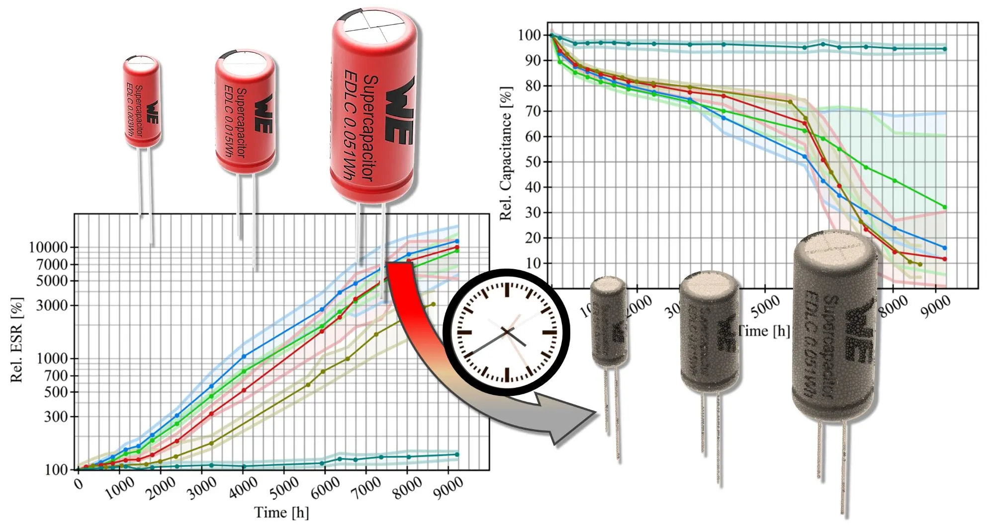
The test comprised batches of 32 pieces of commercial EDLCs with capacitances of 3 F, 15 F, 50 F, and 350 F from Würth Elektronik, as detailed in . The relevant materials of the capacitors are similar. They comprise an activated carbon electrode with polymer binder, Cellulose paper, quaternary ammonium salt, and organic solvent. The 3 F to 50 F types were standard cylindrical capacitors with leads, and the 350 F types were cylindrical snap-in capacitors. The test duration at 65 °C and room temperature (about 24 °C) was about 9,000 h (≈1 year) and 35,000 h (≈4 years), respectively. The 3 F, 15 F, and 50 F types were soldered onto PCBs, each holding 16 pieces. Due to their larger size, the 350 F EDLCs have been soldered to 4 PCBs, each carrying 8 parts. Board-to-board connectors connected the PCBs via a fixture to a DC voltage source, which permanently applied the rated voltage of 2.7 V. To study high-temperature storage, 32 pieces of the 50 F type were kept under short-circuit conditions.
For the measurement, the PCBs were connected to a fixture utilizing the same connector type, allowing easy change between the voltage source and measurement fixture. The measurement fixture was connected by 16 parallel channels to a Chroma 17011 charge/discharge tester (10 V, 6 A per channel). The 2 m long leads do not negatively influence the constant current measurement, since the equipment utilizes a four-terminal Kelvin configuration. All lines and terminals meet the manufacturer’s specifications for the measuring device.
To minimize temperature variations of the device during the test (at 65 °C), both the charging fixture and the measurement fixture were permanently placed in a DY110 climate chamber from ACS Angelantoni Test Technologies, operated as an oven (no humidity control). The chamber was briefly opened for measurement, and the boards were switched from one fixture to another. After a short time to ensure temperature equilibrium, the constant current measurement was conducted to acquire the capacitance and the ESR i.a.w. IEC 62391. In addition to the high-temperature test, tests at room temperature have been performed with 32 pcs of 3 F and 50 F, which were placed in the laboratory. The laboratory is equipped with air conditioning that was operated during summer days to avoid strong deviations from the average room temperature of about 24 °C. Both the tests at room temperature and 65 °C were performed with the same equipment and procedures.
.
Overview of tested samples.
| Capacitance, Part Number |
Test at 65 °C,
2.7 V |
Test at 65 °C,
0 V |
Test at Room Temp. (24 °C), 2.7 V |
| 3 F, 850617030001 |
32 |
/ |
32 |
| 15 F, 850617021005 |
32 |
/ |
/ |
| 50 F, 850617022002 |
32 |
32 |
32 |
| 350 F, 851617034001 |
32 |
/ |
/ |
During the measurement each capacitor was measured once, creating a population of capacitance and ESR values at a given time. Based on this data set, the median as well as the 10th percentile and 90th percentile were determined at each time of measurement. The measurements of 3 capacitors, which were damaged due to operational user errors, are neglected in the analysis. To find an objective means to exclude those parts, the upper 10% and the lower 10% of the sample space were systematically neglected.
6. Results and Discussion
This section presents and discusses measurements made under the above-described conditions. The discussion includes the interpretation of the data, with deterioration mechanisms described in the literature, and the calculation of apparent acceleration factors by comparing measurements made at different temperatures.
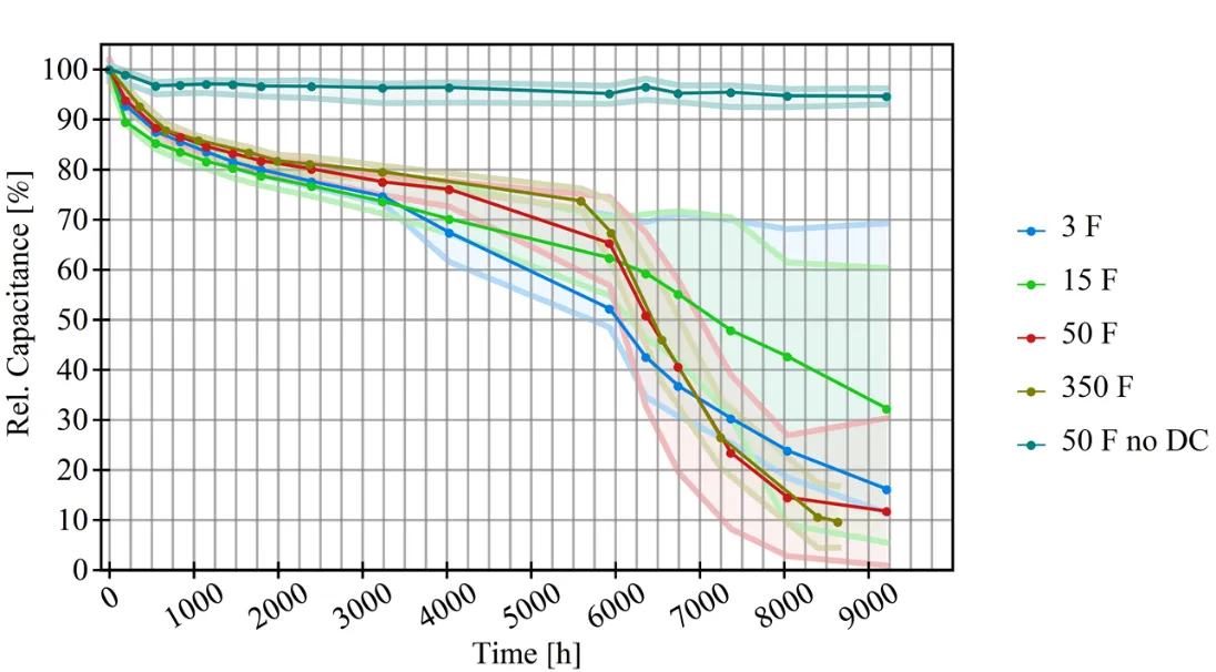
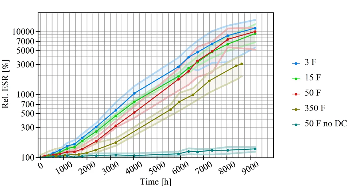
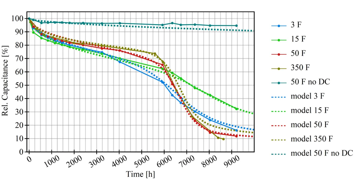
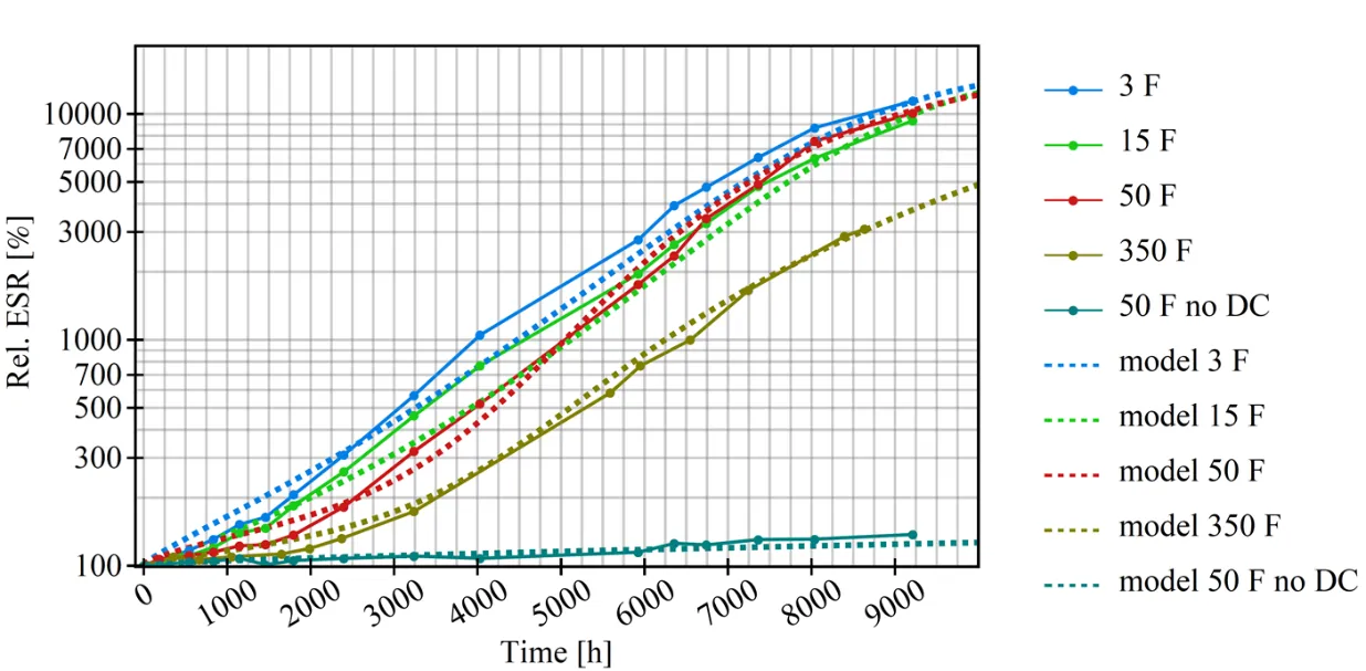
The average relative capacitance and ESR, measured over a range of about 9000 h at 65 °C, are plotted in and , respectively, and show a substantial deterioration for EDLCs with applied voltage and a more moderate decline for the short-circuited sample. The semitransparent area along the graph indicates the 10th percentile and 90th percentile. The capacitance for the parts that were permanently kept at their rated voltage of 2.7 V decreases well below 40% relative to their initial value. The corresponding ESR of those parts has deteriorated to more than tenfold relative to their initial value. The short-circuited parts, however, are still well within the EOL criteria.
. Median relative capacitance <i>vs.</i> time for different batches of capacitor types tested at 65 °C. The 3 F, 15 F, 50 F and 350 F types were permanently kept at 2.7 V. One batch of 50 F types was permanently short-circuited. The semitransparent area marks the 10th percentile and 90th percentile.
The parts have a defined EOL at 30% capacitance loss and 100% ESR increase relative to their rated parameters. The datasheet endurance is guaranteed for 1000 h at 65 °C and with an applied voltage of 2.7 V. All parts are well within the EOL limits for the endurance time. The dispersion of the capacitance and ESR values increases with time. The mean average deviation for the capacitance and ESR measurements is about 40% and 30%, respectively. Especially above 3000 h, the dispersion is well above 10%, indicating a dispersion in aging rates and thus highlighting that any aging or degradation forecast can only be an estimate, even for highly standardized commercial parts. This increasing dispersion at large measurement times may be identified as the wearout phase, in which the failure rate rises rapidly [
28]. Usually, wearout only occurs for electronic devices beyond the service life,
i.e., above the EOL criteria. Unfortunately, based on this study, it is not possible to identify the physical or electrochemical mechanisms responsible for the wearout.
Commonly, EDLCs have production tolerances around 40% and are typically delivered with capacitances slightly above the rated value. Therefore, the measured dispersion of <10% below the EOL criteria is within this limit and could be assessed as acceptable. This phase may be identified as the early-life or steady-state phase, in which failures occur at a decreasing or constant rate [
28]. The reliability prediction assumes that within the early life, which is well below EOL criteria, the failure rate is constant and the lowest within the life cycle of electronic equipment.
. Median relative ESR <i>vs.</i> time for different batches of capacitor types tested at 65 °C. The 3 F, 15 F, 50 F, and 350 F types were permanently kept at 2.7 V. One batch of 50 F types was permanently short-circuited. The semitransparent area marks the 10th percentile and 90th percentile.
The general progression of the capacitance values
vs. time, as shown in , is comparable to measurements previously reported in the literature [
7,
23,
26]. Slight discontinuities arise from variations associated with the measurement. Usually, the capacitance decreases in the first phase, lasting around 1000 h to 3000 h, with a power law or square root time dependence. Literature associates this degradation with electro-thermal degradation of electrolytes and or loss of electrode surface area [
18,
23].
The second phase, which starts above 4000 h to 5000 h or so, is not well-documented but is still discussed or hinted at in some publications. [
26,
43] It is speculated that the second phase,
i.e., wearout phase, is associated with further loss of active electrode area and the decrease of potential barrier between electrolyte and carbon electrode interface [
26,
43]. Since the loss of electrolyte is challenging to detect, it might be that the lack of availability of conducting ions is an additional cause for the device performance [
42].
The ESR in increases over several orders of magnitude. For the 3F and 50 F types, the rate of ESR increase seems to accelerate around 1000 h and to decelerate slightly around 8000 h. Below 6000 h, the relative change in ESR and capacitance for large capacitor types is lower than for smaller capacitor types,
i.e., larger capacitor types degrade more slowly than smaller ones. The short-circuited 50 F capacitors degrade much more slowly than the capacitors charged at the rated voltage of 2.7 V, showing that without voltage, the degradation is reduced significantly but not entirely.
This may allow speculation that the volume loss of electrolytes could contribute to the degradation [
42]. Smaller capacitors may be subject to a larger loss of electrolyte relative to their housing size. Additionally, the type of sealing may also have an effect. The 350 F type is a snap-in design with a roll-fold sealing that secures the baseplate and the container, providing better sealing than the rubber stopper of the standard cylindrical design. However, at this point, this is speculation; the loss of electrolyte by evaporation needs to be determined in another gravimetrical experiment.
Although this study does not include chemical or physical analysis and therefore does not allow for discussions concerning the deterioration mechanism, others have studied this area in detail. The decrease in capacitance and increase in ESR could be attributed to the agglomeration of conductive carbon particles and the reduced crystallinity of the carbon materials, but also to the erosion of the current collector itself and the delamination between the collector and the activated carbon [
5]. The erosion is caused by electrochemical decomposition of the activated carbon, a more pronounced process in the anode than in the cathode. The performance degradation of the supercapacitor could thus be attributed to the reduced ion diffusion efficiency in the collapsed, blocked, or narrowed pores of the activated carbon layer and the separator, which in this study was a polypropylene film. Sedlakovas’ study on diffuse resistance corroborates these results [
26].
Concerning the usability of the capacitors, the test results indicate that even after the datasheet endurance limit of 1000 h, the capacitors are still functioning. Applications requiring a current demand below the rated voltage could tolerate an increase of ESR above the EOL limit. The decision on what an acceptable degradation is can only be made if the power demand of the application is known. However, by moderate oversizing, knowing the degradation rate could enable the engineer to prolong the estimated lifetime of the application and thus save resources. Choosing a larger capacitor adds an extra cost but might be environmentally and financially less costly than replacing the entire device.
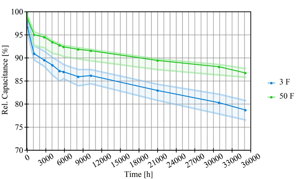
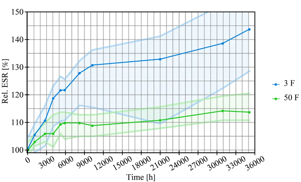
To assess the extrapolation of the degradation to lower temperatures, 3 F and 50 F capacitor types have been tested at room temperature,
i.e., about 24 °C. The median of the resulting capacitance and ESR measurements, taken over 4 years, is given in and , respectively, and illustrates that the device parameters are within the EOL criteria, which are defined as 30 % capacitance loss and 100 % ESR increase. As for and , the semitransparent area in and indicates the 10th percentile and 90th percentile value.
. Median relative capacitance <i>vs.</i> time for different batches of capacitor types tested at room temperature, <i>i.e.</i>, 24 °C, and permanently applied DC voltage of 2.7 V. The semitransparent area marks the 10th percentile and 90th percentile.
. Median relative ESR <i>vs.</i> time for different batches of capacitor types tested at room temperature, <i>i.e.</i>, 24 °C, and permanently applied DC voltage of 2.7 V. The semitransparent area marks the 10th percentile and 90th percentile.
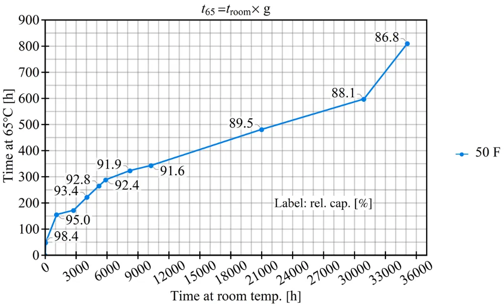
Within the capacitance decrease of about 20% and for the ESR increase of about 40%, the long-term measurements at 65 °C and 24 °C allow the calculation of the temperature factor. Let $$C_{0} \left(t_{0} ; T_{0}\right)$$ and $$E S R_{0} \left(t_{0} ; T_{0}\right)$$ be the relative capacitance and ESR, respectively, at time $$t_{0}$$ for a given temperature $$T_{0}$$ and $$C_{1} \left( t_{1} ; T_{0} g \left(T\right) \right)$$ and $$E S R_{1} \left( t_{1} ; T_{0} g \left(T\right) \right)$$ the relative capacitance and ESR, respectively, at time $$t_{1}$$ for a given temperature $$T_{1}$$ then $$C_{0} \left(t_{0} ; T_{0}\right) = C_{1} \left( t_{1} g ; T_{1} \right)$$ and $$E S R_{0} \left(t_{0} ; T_{0}\right) = E S R_{1} \left( t_{1} g ; T_{1} \right)$$ with $$t_{0} = t_{1} g$$. This calculation can be done numerically by rescaling the time axis of an interpolated function of $$C_{0}$$ and $$E S R_{0}$$ until the $$C_{0} = C_{1}$$ and $$E S R_{0} = E S R_{1}$$. The thermal acceleration factor $$g$$ can be determined independently based on the capacitive and resistive changes. For the sake of simplicity, a subscript for $$g$$, indicating the type of measurement, is not introduced. A graphical example for the determination of $$g$$ is shown in Appendix B in Figure A3.
The measurements for $$T_{0} = 65$$ °C, given in
as well as
, and for $$T_{1} = 24$$ °C (room temperature), given in
and
are used to calculate the factor stepwise.
and
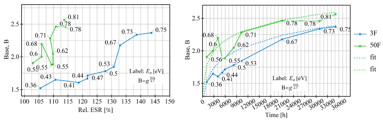
shows $$B = g^{\frac{10 K}{\Delta T}}$$ as well as the activation energy $$E_{a} = log \left(g\right) k_{B} \frac{\Delta T}{T_{1} T_{0}}$$ versus measurement time and relative deterioration as calculated from the capacitance (
and
) and ESR (
and
) measurements, respectively. The capacitance, as well as the ESR measurement, yields about the same results in terms of base and activation energy, which is given in units of eV as plot marker annotations. The range of the activation energies, as well as the base for the corresponding acceleration factor, is comparable to literature values [
23,
30,
31].
. Plot of base <i>B</i> <i>vs.</i> rel. capacitance (left) and <i>B</i> <i>vs.</i> time (right) as calculated from the capacitance measurement for the 3 F type and the 50 F capacitors. The labeled plot markers give the corresponding activation energies according to Arrhenius law in units of electron volts (eV). The dotted lines represent fits introduced in Section 7 (Figure$$\,$$ 9).
. Plot of base <i>B</i> <i>vs.</i> rel. ESR (left) and <i>B</i> <i>vs.</i> time (right) as calculated from the ESR measurement for the 3 F type and the 50 F type. The labeled plot markers give the corresponding activation energies according to Arrhenius law in units of electron volts (eV). The dotted lines represent fits introduced in Section 7 (Figure$$\,$$10).
Apart from the unsteady behavior for the ESR-based measurements around 3000 h, it is generally noticeable that $$B$$ and $$E_{a}$$, increase with time,
i.e., with relative deterioration of the device. It suggests that the effect of $$\Delta T$$ increases with time and an acceleration factor $$\propto 2^{\left(\frac{\Delta T}{10 K}\right)}$$ could be considered an estimate. In this measurement, the 50 F capacitor type has, on average, larger activation energies than the 3 F type. Hence, the temperature is reduced below the max. temperature (65 °C), as used in the endurance test, will tend to a stronger gain in lifetime for the 50 °F-type than for the 3 °F-type. An acceleration factor with deterioration-dependent or time-dependent activation energy would be required to get an exact description of the deterioration over time.
The flattening of the slope of the function $$B$$ with the increase of measurement time in
and
may indicate a limit, and that for larger deteriorations and measurement times, $$B$$ indeed can be well approximated by a constant. This set of measurements suggests that the widely used base of $$B = 2$$ for the temperature factor is a lower estimate that best fits deterioration well below the EOL conditions of EDLCs. This is a conservative estimate for the product’s reliability, which might tend to underestimate the lifetime at lower temperatures.
Whether or not a deterioration or time-dependent description is necessary is open for discussion; after all, lifetime calculations are estimates, and the application’s operational parameters are rarely precisely known. Also, the production tolerances of EDLCs are about 40%, so one could argue that the current approach is sufficiently precise. On the other hand, using an unsuitable acceleration factor may lead to overestimating the lifetime.
The time periods during which these studies are conducted, and the number of samples, make it challenging to test at several temperatures. In this campaign, it was therefore only possible to test at 65 °C and room temperature. Indeed, the validity of the data can be enhanced when tested against other long-term experiments conducted at different temperatures. However, the collected data proves that the apparent activation energies are not constant (see Section 3). If a non-constant apparent activation energy is found for these two temperatures, then it is plausible to assume that it could also be true for other temperatures.
Based on the reviewed literature and the above discussion, finding a model based on electrochemical or physical principles and mechanisms appears challenging. Presumably, the complexity of the processes makes it difficult to formulate an approach leading to a closed mathematical expression. There are certainly estimations possible, concerning the temperature dependence, based on the Arrhenius theory, utilizing apparent activation energies. However, those appear only valid for a certain time or deterioration regions. Thus, closed mathematical expressions, which have the advantage of being relatively easily implementable, may currently only be found phenomenologically. Although such models do not give any insights into the physical processes, they can express device and environmental characteristics by a set of parameters. The challenge is to find an accurate model that describes all features of the deterioration behavior with a small set of parameters.
In the next section, a phenomenological description $$B$$
vs. time, as well as the exponents $$t^{∗} A \left(t^{∗}\right)$$ are introduced to give a mathematical approximation of the measurement, allowing for a more precise degradation forecast.
7. Measurement Modeling
In the previous sections, the general deterioration model and the long-term measurements and their discussion have been introduced. As already mentioned, the deterioration model and the acceleration factor require adaptation to actual measurements. These mathematical adaptations are discussed in the following section.
Especially the time-dependent exponent $$t A \left(t\right)$$ of the deterioration model in
Equation (15) and
Equation (16), but also the base $$B \left(t\right)$$ for the temperature acceleration factor have to be phenomenologically determined based on the measurement values. Although the equations below allow a description of the measured data, they might not be the only conceivable approach; they present just one possible approach.
The phenomenological approach
with $$q$$ and $$r$$ as form parameters for the adjustment of the graph, allows a rough description of the base, as is printed in
and
for the capacitance and ESR measurements, respectively, using the parameters given in Table A2 (Appendix D). The proposed function $$B \left(t\right)$$ is heuristically constructed and not directly related to any electrochemical or physical model but allows the description of the measurements with a small parameter set.
With
Equation (17) the corresponding time-dependent acceleration factor is
In the course of this paper, Equation (18) is used to assess the influence of a variable base,
i.e., activation energy, on predictions made by the model introduced in Section 4.
The exponents $$t^{∗} A_{c} \left(t^{∗}\right)$$ and $$t^{∗} A_{\sigma} \left(t^{∗}\right)$$ in the deterioration models, given in
Equation (15) and
Equation (16), respectively, contain time-dependent exponential deterioration rate factors $$A_{c} \left(t^{∗}\right)$$ and $$A_{\sigma} \left(t^{∗}\right)$$. The time dependence is motivated by the different phases, which exhibit varying deterioration rates resulting from distinct degradation mechanisms. Although the exact cause of the degradation mechanism is not entirely clear, it is possible to find a function that gives a phenomenological description of the degradation. One type of function that allows modeling of different phases is sigmoid-like functions, which can be expressed with the trigonometric $$\mathrm{tanh} \left(x\right)$$. It was found that the exponent
with
and with $$a$$ as a constant, proportional to the overall gradient, $$t_{1}$$ as the position of the first phase, $$t_{2}$$ as the onset of the second phase, $$b_{1}$$ and $$b_{2}$$ as factors governing the magnitude of the first and second deterioration phase, respectively, $$p_{2}$$ as a factor governing the steepness of the onset of the second phase, can be used as a general approach to describe time-dependent deterioration.
The function is entirely phenomenological, as is explained in Appendix C, and has the advantage that all parameters are directly related to properties of the degradation curves, such as positions of phases or gradients of slopes. The above-presented explicit function for $$t^{∗} A \left(t^{∗}\right)$$,
i.e., $$t^{∗} A_{c} \left(t^{∗}\right)$$ or $$t^{∗} A_{\sigma} \left(t^{∗}\right)$$, is not necessarily the only one that could be used as a time-dependent exponent in
Equation (15) and
Equation (16); however, it serves the purpose of describing the measurements as shown in
and
with a mean absolute percentage error (MAPE) ranging from 2% to 15%. The error and model parameters are listed in the Table A3 and Table A4 (in Appendix D) for the capacitance and ESR measurements, respectively. Based on the mean average deviations of up to 40% and 30% for capacitance and ESR measurements, respectively, the model is accurate enough to be considered an appropriate estimate. The parameters for the temperature and voltage acceleration factors are: $$s = 0 . 73 \,\mathrm{V} $$ as fitting factors, $$V_{r} = 2 . 7 \,\mathrm{V}$$ as rated voltage and $$T_{0} = 65{\,}^{\circ}\mathrm{C}$$ as reference temperature.
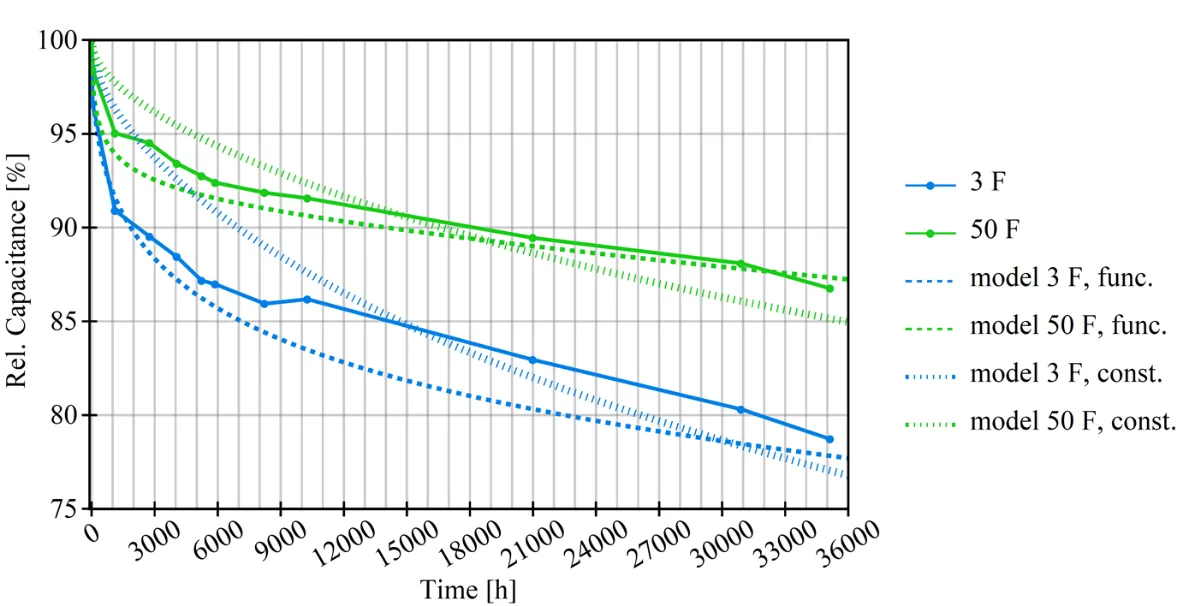
. Relative capacitance <i>vs.</i> time for different batches, as introduced in , with corresponding models. The parameters used for the model calculations are given in Table A3.
The model describing the capacitance as well as the ESR for the short-circuited 50 F batch (50 F No DC) uses the same parameter set as for the 50 F batch (see Table A3 and Table A4 in Appendix D) with the exception of the operating voltage, leading to the rescaling of the time by the factor $$h \left( V \right)$$. The model describes the capacitance as well as the ESR with a MAPE of about 2 % and 4 %, respectively, and could be considered a good estimate.
The influence of certain model parameters will be discussed using the example of capacitance measurement. The position $$t_{1} \times 24 \times 365 \approx 2000$$ h marks the onset of the “steady phase” (see Appendix C), which is about the same for all measured capacitors. Within this phase, the larger capacitor types degrade more slowly than the smaller ones, which is reflected in the constant $$a$$, introduced as the overall gradient. The position of the shoulder, related to the second degradation process, $$t_{2} \times 24 \times 365 \approx 7000$$ h is also roughly equal for all capacitors. The rate of decay, plotted in Figure A5 (right-hand side), is lowest between $$t_{1}$$ and $$t_{2}.$$ An increase in $$a$$ leads to an overall increase in the deterioration rate, while $$b_{1}$$ and $$b_{2}$$ are related to the increase of the deterioration rate of the first and second phases, respectively. A substantial difference exists between the second phase degradation of the 15 F-type and 350 F-type, which is reflected in a larger $$b_{2}$$ for the 350 F-type than for the 15F-type (Table A3).
. Relative ESR <i>vs.</i> time for different batches, as introduced in , with corresponding models. The parameters used for the model calculations are given in Table A4.
and show that the proposed model can describe the degradation in the early phase and when the parts are strongly degraded above 5000 h or so. A linear or square root dependence may be able to capture the degradation behavior of early life degradation (1000 h to 3000 h), but not the late degradation phases [
15,
19]. A Similar statement could be made about approaches that involve combinations of power law and linear functions in time [
24]. Beyond a specific time, those functions cannot fit the data or produce even physically unreasonable results, since they are unbounded.
Exponential functions are, in principle, capable of fitting degradation curves for extended periods, as was shown by Sedlakova, using separate functions with a square root and Gaussian-like exponents [
26]. Hence, the above-mentioned approaches are suitable for describing individual phases but not the entire early and late lifetime degradation within one expression. However, the proposed approach in this paper aims to be more general. It introduces an exponential function with an exponent that can capture the changing degradation rates over time, as is illustrated in and . As a result, this approach may benefit from a more accurate long-term prediction of degradation.
The comparison of the capacitance and ESR models against measurements taken over about 4 years is given in
and
, respectively. The model calculations, plotted in
, for the capacitive decline are made with a temperature factor using a constant base $$B_{3 F}^{C} = 2 . 1$$ for the 3 F capacitor types and $$B_{50 F}^{C} = 2 . 5$$ (superscript of $$B$$ indicates the type of measured parameter, measurement and subscript indicates the capacitor type) for the 50 F types as well as in the
Equation (18) introduces time-dependent temperature factors. The constants have been chosen to fit the values of approximately 15,000 h to 18,000 h in the mid-time region. Using the more accurate time-dependent model of the temperature factor leads to an MAPE of about 1 % for the 3 F and 50 F types, while the constant base leads to MAPEs of 3% and 2 %, respectively. The model involving the time-independent base overestimates the capacitance for times below the mid-term region and underestimates the measured values above the mid-term region. This demonstrates that the base values chosen from the evaluation in
and
indeed lead to a good fit around that measurement time,
i.e., the corresponding degradation.
This measurement set can also demonstrate that the presented modeling approach aligns with the acceleration factor-based lifetime calculation. In those calculations, the endurance time is extrapolated with an acceleration factor [
21]. The endurance time measurement is conducted for a specific time and relates to a particular state of degradation, under stressed conditions. Datasheets, for instance, state the endurance measurement time to provide engineers with the reference time under stressed conditions. The correspondence between the model and the acceleration factor-based lifetime calculation can also be exemplified by a calculation using the time at 90% degradation as measured for 65 °C for the 50 F type, which is approximately 920 h (
), which serves as a reference time in this example. For the 50 F type, a temperature factor of basis $$B_{50 F}^{C} = 2 . 5$$ the “accelerated time” is $$\left(920 \,\mathrm{h} \times 2 . 5\right)^{\left( 56{\,}^{\circ}\mathrm{C} - 24{\,}^{\circ}\mathrm{C} \right) / 10 \mathrm{K}} \approx 18 , 000\, \mathrm{h} .$$ This is very close to the measured and calculated degradation of the 50 °F type in
.
. Capacitance of EDLCs measured during long-term measurement at room temperature and rated voltage, model with time-dependent temperature factor (utilizing fits of
Equation (17) given in
) and time-independent factor with $$B_{3 F}^{C} = 2 . 1$$ for the 3 F capacitor type and $$B_{50 F}^{C} = 2 . 5$$ for the 50 F type.
The model calculations for the ESR in
are made with a temperature factor using a constant base $$B_{3 F}^{E S R} = 2 . 2$$ and $$B_{50 F}^{E S R} = 2 . 6$$ for the 3 F type and 50 F type, respectively, and a time-dependent temperature factor, leading to MAPEs of around 7 % and 2 %, respectively. Using the time-dependent temperature factor, the degradation model describes the actual measurements, with an MAPE of about 2 % and 1 % for 3 F type and 50 F type, respectively. As for the capacitance measurement, the constant base of $$B_{3 F}^{E S R} = 2 . 2$$ and $$B_{50 F}^{E S R} = 2 . 6$$ leads to underestimation below the region of about 15,000 h to 18,000 h and overestimation above this region.
. ESR of EDLCs measured during long-term measurement at room temperature and rated voltage, model with time-dependent temperature factor (utilizing fits of
Equation (17) given in
) and time-independent factor with $$B_{3 F}^{E S R} = 2$$.2 for the 3 F type and $$B_{50 F}^{E S R} = 2 . 6$$ for the 50 F type.
The time-dependent factor generally describes the progression of the capacitance and ESR measurements better than the time-independent factor. The latter, however, can fit the measurement well for a specific point in time or degree of degradation and may therefore still be used as a proper estimate.
The measurements do not reveal the cause of the change in activation energies. However, they could suggest that the distribution of apparent activation energies might be influenced by degradation of the EDLCs, caused, for instance, by deterioration of the electrode effective surface,
i.e., pores [
8,
36].
Degradation apparently cannot be ascribed to one single process. Electrochemical reaction at the electrode interface, loss of liquid electrolyte by phase transition, deterioration of the electrode system and deterioration of the housing parts, such as rubber seals, can have an effect. At this point, it appears plausible that the measured deterioration involves multiple mechanisms leading to different phases of aging as well as a distribution of apparent activation energies.
8. Conclusions and Outlook
The long-term measurements of capacitors at a temperature of 65 °C and room temperature and a permanently applied DC voltage of 2.7 V show two phases of degradation. The rate of capacitance loss in the second phase, starting at about 5000 h, is larger than in the first phase. Possible degradation mechanisms have been discussed based on the literature. A control group of short-circuited capacitors shows only weak deterioration, indicating that decreased voltages can at least partially compensate for the degradation effects of temperature. The proposed phenomenological model, in combination with a time-dependent temperature acceleration factor, can describe deterioration curves at two different temperatures and voltages. It can describe the deterioration over the entire life span of the tested capacitors and may serve as a tool to predict device deterioration at all life phases.
The comparison of the accelerated tests at 65 °C and the long-term measurements at room temperature, which lasted for about 4 years, showed that the temperature factor changed over time. The time-independent factor may serve as an estimate, but the model’s accuracy is increased if the time-dependent temperature factor is used. The change in activation energy suggests that deterioration is not driven by a single electrochemical process, but rather by multiple mechanisms. Further measurements at different temperatures are needed to verify the change in the activation energy, which is merely an apparent activation energy, as discussed in Section 3.
Long-term measurements should be conducted extensively to improve the accuracy of the forecast. While the current acceleration factors may be a tool for estimating lifetime, an improved deterioration model may be actively used during the design to target a particular lifetime by moderate oversizing or to forecast the EOL more accurately. This study suggests that efforts to conduct long-term measurement tests under different stress factors should be resumed to test and improve this deterioration model and the accuracy of acceleration factors. Future studies may reveal an expression of the degradation function directly related to electrochemical processes.
Appendix A
This section provides simplified calculations to illustrate the principle of the model. As an example, the model is calculated based on a constant deterioration rate $$\Delta D_{n}$$ and its relation to the linear model is given.
For short periods, a linear approximation of $$\frac{D}{D_{0}}$$ at position $$t_{a}$$ using the Taylor theorem, denoted as $$\frac{D}{D_{0}} \approx T \left(\frac{D}{D_{0}} , t ; t_{a}\right)$$ yields
or for $$t_{a} = 0$$
which is the same type as
Equation (1). Hence, the exponential model can be transferred to a linear model under the assumption of small relative changes $$\Delta D_{n} \ll 1$$. Equation (A2) also allow the determination of the $$f \left(\Delta t\right) = A \Delta t$$ from the experimental data in the near-linear region. Since small relative changes relate to small periods of time, it is equivalent to say that the exponential model is in good approximation with linear models for small relative changes $$\Delta D_{n} \ll 1$$ or small periods $$\Delta t \ll t$$.
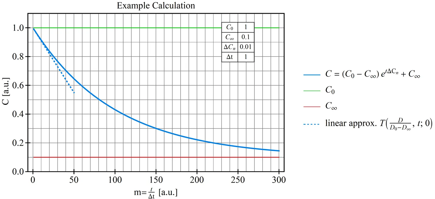
The example of calculation of Equations (15) and (16), which is given in Figure A1 and Figure A2, respectively, illustrate the fundamental progression of aging and the relation to the linear approximation given by Equation (A2). The parameters for the calculations, given in the inset of the figures, are dimensionless and chosen for convenience and illustrative purposes only.
Figure A1. Exemplary calculation of capacitance deterioration.
The capacitive deterioration in Figure A1 starts at a given initial capacitance $$C_{0}$$ and degrades with increasing $$m = t$$ (in this example $$\Delta t = 1$$) towards its residual value $$C_{\infty}$$. Under application-relevant conditions $$C_{\infty}$$ may never be reached since the capacitor would have lost its function far before that point. Around its start point, the exponential function can be approximated linearly and is thus in continuity with existing modeling approaches, as discussed above [
10,
19,
20].
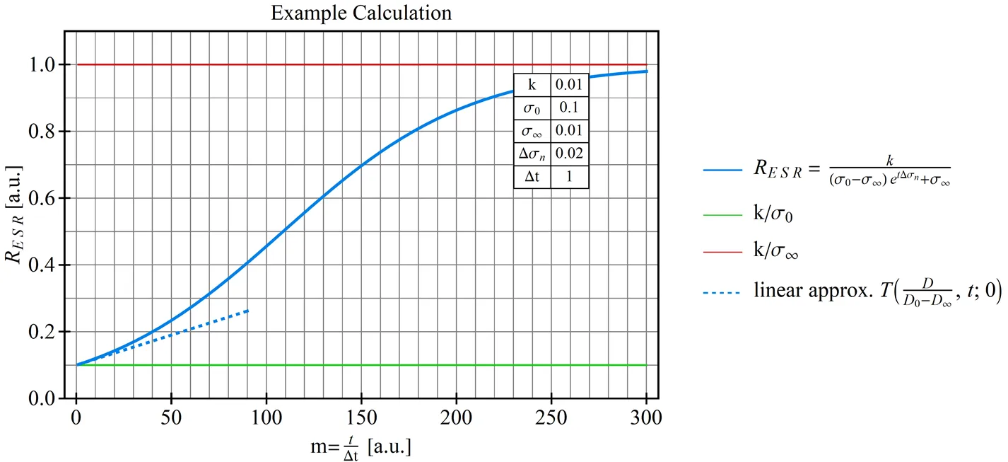
Figure A2. Exemplary calculation of ESR deterioration.
The Sigmoid-like progression of the $$R_{E S R}$$, given in Figure A2, shows its increase from the initial value $$k / \sigma_{0}$$ towards its theoretically possible upper limit $$k / \sigma_{\infty}$$, which in commercial parts corresponds to a high ohmic value that may only be reached during long operation times or because of significant deteriorations. As for the capacitance, also, the degradation of the ESR can be described as a linear function around $$m = t \approx 0$$. Hence, the calculation of the long-term deterioration,
i.e., $$t \gg \Delta t$$, could be performed based on the linear fit of the endurance values, which are measured on a shorter time scale $$\Delta t$$.
Appendix B
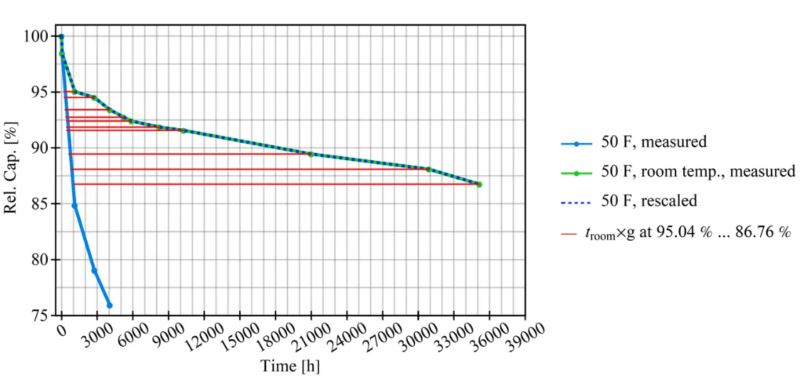
This section exemplifies the calculation of the acceleration factor. Figure A3 and Figure A4 visualizes the scaling of the measurement taken at 65 °C and room temperature (about 24 °C) by the temperature acceleration factor on the example of the 50 F capacitor type. (see also corresponding Table A1) Figure A3 shows the linear interpolation of the measured median
vs. time for the 50 F type and the positions at which it was scaled to meet the measurement points at room temperature. More specifically, if $$C_{65} \left(t \times g\right)$$ and $$C_{r o o m} \left( t \right)$$ is the linearly interpolated measured capacitance at 65 °C and room temperature, respectively, then $$g$$ is the factor under which $$C_{65} \left(t \times g\right) = C_{r o o m} \left( t \right)$$. In this manner, for each point,
i.e., red line, a scaling factor $$g $$ is derived, from which the activation energy $$E_{a}$$ and the base $$B$$ can be calculated. With the above definition of $$g$$ the red line is proportional to $$g^{- 1}$$. A small error may occur due to the linear interpolation of the high temperature measurement.
Figure A3. Visualized rescaling of the measurement taken at 65 °C to meet the values measured at room temperature. Intermediate points of the high temperature measurement were linearly interpolated.
Figure A4 shows that the time scaling for different relative capacitances between the measurement at 65 °C and the one taken at room temperature is not linear. As time increases,
i.e., the relative capacitance decreases, the scaling between the time at room temperature and elevated temperature increases in the sense that for $$t_{r o o m} = g^{- 1} t_{65}$$ the scaling factor $$g^{- 1}$$ increases.
Figure A4. Time scaling under different temperature conditions for capacitance measurement of the 50 F capacitor type.
The temperature acceleration factor $$g$$ maps, or rescales, the time axes of the measurement taken at 65 °C to the one at room temperature and vice versa, as is shown in Figure A3. This analysis was performed similarly for the other capacitance and ESR measurements of the 3 F and 50 F types.
Table A1.
Summary of relative capacitances and corresponding measurement time, $$g$$, $$E_{a}$$, $$B$$ as retrieved from the measurement plotted in Figure A3 for $$T_{0}$$ = 56 °C (338 K) and $$T_{1} $$= 24 °C (297 K) with $$k_{B} = 8 . 617 \times 10^{- 5}\, \mathrm{e V K}^{- 1}$$.
| Relative Capacitance [%] |
Time [h] |
Temperature Acceleration Factor, $$\bm{g}^{- 1}$$ |
Temperature Acceleration Factor, $$\bm{g}$$ |
Activation Energy,
$$\mathbf{log} \left(\bm{g}\right) \bm{k_{B}} \frac{\bm{T}_{0} \bm{T}_{1}}{\bm{\Delta} \bm{T}} = \bm{E}_{\bm{a}} \bm{ }\,$$[eV] |
Base,
$$\bm{B} = \bm{g}^{10 \bm{k} / \mathbf{\Delta} \bm{T}}$$ |
| 95.04 |
1113 |
7.15 |
0.140 |
0.42 |
1.62 |
| 94.51 |
2760 |
16.01 |
0.062 |
0.59 |
1.97 |
| 93.42 |
4056 |
18.22 |
0.055 |
0.61 |
2.03 |
| 92.75 |
5232 |
19.67 |
0.051 |
0.63 |
2.07 |
| 92.40 |
5880 |
20.34 |
0.049 |
0.64 |
2.09 |
| 91.86 |
8232 |
25.39 |
0.039 |
0.68 |
2.20 |
| 91.56 |
10,272 |
29.89 |
0.033 |
0.72 |
2.29 |
| 89.45 |
21,000 |
43.60 |
0.023 |
0.80 |
2.51 |
| 88.09 |
30,912 |
51.72 |
0.019 |
0.83 |
2.62 |
| 86.76 |
35,136 |
43.34 |
0.023 |
0.80 |
2.51 |
Appendix C
This section intends to plausibilize
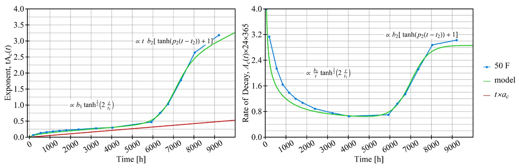
Equation (19), which is phenomenological and heuristically constructed to describe the measured change in the exponential term, which appears to have two phases. The motivation to use this particular equation shall be explained briefly on the example of measured capacitance deterioration of the 50 F type, which is referred to as $$C_{m}$$. Any time-dependent exponent would have to fit the $$- \mathrm{log} \left(C_{m}\right)$$ graph, which is plotted in Figure A5. Heuristically one would seek a function that is able to describe this slowly increasing step-like behavior. Such a function could be a linear combination of the tanh function. The tanh-function is bounded, well implemented in most calculation software and its shape,
i.e., the steepness and position of its shoulder and upper and lower bound, can be directly changed by parameters, as explained in Section 7. Each phase of the measured capacitance is described by the two tanh-terms, as is illustrated Figure A5, which shows the corresponding exponent of the measured data $$- \mathrm{log} \left(C_{m}\right)$$, the fit of
Equation (19) and for comparison with linear time scaling $$t\, a_{C} .$$
As a result, the decay rate $$A \left(t\right)$$, also shown in Figure A5 has a bathtub-like shape. The first phase, which includes an increased decay rate at the beginning, is followed by a “steady-state” period, signified by the bottom of the bathtub curve. The increase in the curve indicates the second phase, with its accelerated decay. The scaling $$24 \frac{\mathrm{h}}{\mathrm{d a y}} \times 365 \frac{\mathrm{d a y}}{\mathrm{y e a r}}$$ (
y-axis) has been introduced without loss of generality for numerical convenience only.
Future research may focus on the formulation of models that directly relate to physical or chemical processes that result in the behavior displayed in the graphs.
Figure A5. Plot of exponent <i>vs.</i> time (<b>left</b>) and plot of rate of decay <i>vs.</i> time (<b>right</b>) as measured and modeled for the 50 F type.
Appendix D
Table A2.
Parameter for the fit of the time-dependent base $$B .$$
|
Based On Capacitance |
Based on ESR |
| type |
$$q$$ |
$$r$$ |
$$q$$ |
$$r$$ |
| 3 F |
0.028 |
0.3 |
0.03 |
0.32 |
| 50 F |
0.019 |
0.4 |
0.058 |
0.28 |
Table A3.
Model parameters are used in Figure 7 and mean absolute percentage error (MAPE) of the model and measurement. The scaling $$24 \frac{\mathrm{h}}{\mathrm{d a y}} \times 365 \frac{\mathrm{d a y}}{\mathrm{y e a r}}$$ (y-axis) has been introduced without loss of generality for numerical convenience only.
| Data Set |
$$\bm{a} \times \mathbf{24} \times \mathbf{365}$$ |
$$\frac{\bm{t}_{\mathbf{1}}}{\mathbf{24} \times \mathbf{365}}$$ |
$$\frac{\bm{t}_{\mathbf{2}}}{\mathbf{24} \times \mathbf{365}}$$ |
$$\bm{b}_{\mathbf{1}}$$ |
$$\bm{b}_{\mathbf{2}}$$ |
$$\bm{p}_{\mathbf{2}}$$ |
V [V] |
T [°C] |
MAPE [%] |
| 3 F |
0.527 |
0.25 |
0.80 |
0.25 |
1.40 |
5.00 |
2.70 |
65.00 |
3.99 |
| 15 F |
0.561 |
0.28 |
0.91 |
0.28 |
0.60 |
5.00 |
2.70 |
65.00 |
2.00 |
| 50 F |
0.463 |
0.20 |
0.80 |
0.20 |
2.50 |
10.00 |
2.70 |
65.00 |
3.17 |
| 50 F, No DC |
0.463 |
0.20 |
0.80 |
0.20 |
2.50 |
10.00 |
0.00 |
65.00 |
2.17 |
| 350 F |
0.277 |
0.30 |
0.80 |
0.50 |
3.50 |
10.00 |
2.70 |
65.00 |
14.04 |
Table A4.
Model parameters as used in Figure 8 and mean absolute percentage error (MAPE) of the model and measurement. The scaling $$24 \frac{\mathrm{h}}{\mathrm{d a y}} \times 365 \frac{\mathrm{d a y}}{\mathrm{y e a r}}$$ (y-axis) has been introduced without loss of generality for numerical convenience only.
| Data Set |
$$\bm{a} \times \mathbf{24} \times \mathbf{365}$$ |
$$\frac{\bm{t}_{\mathbf{1}}}{\mathbf{24} \times \mathbf{365}}$$ |
$$\frac{\bm{t}_{\mathbf{2}}}{\mathbf{24} \times \mathbf{365}}$$ |
$$\bm{b}_{\mathbf{1}}$$ |
$$\bm{b}_{\mathbf{2}}$$ |
$$\bm{p}_{\mathbf{2}}$$ |
V [V] |
T [°C] |
MAPE [%] |
| 3 F |
2.190 |
0.30 |
0.50 |
0.05 |
1.00 |
1.00 |
2.70 |
65.00 |
13.66 |
| 15 F |
0.876 |
0.20 |
0.50 |
0.02 |
3.30 |
1.00 |
2.70 |
65.00 |
10.80 |
| 50 F |
1.314 |
0.20 |
0.50 |
0.10 |
1.50 |
4.00 |
2.70 |
65.00 |
10.63 |
| 50 F, No DC |
1.314 |
0.20 |
0.50 |
0.10 |
1.50 |
4.00 |
0.00 |
65.00 |
3.33 |
| 350 F |
0.876 |
0.20 |
0.50 |
0.05 |
1.60 |
4.00 |
2.70 |
65.00 |
7.93 |
Acknowledgments
This research would not have been possible without the technical expert Eric Fischer, and Jon Izkue-Rodriguez at the Würth Elektronik Competence Center Berlin, who provided technical support. Thanks to Jonas Bux and Philipp Mell from the University of Stuttgart for their valuable feedback.
Ethics Statement
Not applicable.
Informed Consent Statement
Not applicable.
Data Availability Statement
The raw digital data supporting the results of this study are available from the author upon reasonable request and are subject to a confidentiality agreement with Würth Elektronik eiSos GmbH. The raw digital data are the property of Würth Elektronik eiSos GmbH.
Funding
This research received no external funding.
Declaration of Competing Interest
The author declares that he has no known competing financial interests or personal relationships that could have appeared to influence the work reported in this paper.
Footnotes
- 1.
-
When changing the base of $$g = e^{\frac{E_{a}}{k_{B}} \frac{\Delta T}{T_{0} T_{1}}}$$ to $$g = B^{\frac{E_{a}}{k_{B}} \frac{\Delta T}{T_{0} T_{1}} \frac{1}{\mathrm{log} B}}$$ then from $$B^{\frac{E_{a}}{k_{B}} \frac{\Delta T}{T_{0} T_{1}} \frac{1}{\mathrm{log} B}} = B^{\frac{\Delta T}{10 K}}$$ follows that $$B = e^{\frac{E_{a}}{k_{B}} \frac{10 K}{T_{0} T_{1}}}$$. Since, $$T_{0}$$ and $$T_{1}$$ are given on the absolute Kelvin scale $$0 \approx \frac{\Delta T}{T_{0}} = \frac{T_{1}}{T_{0}} - 1$$ and the term $$T_{1} T_{0} \approx c o n s t .$$ The relative error $$E$$ of the with $$\left(T_{1} - T_{0}\right) / \left(T_{0} T_{1}\right) \approx \Delta T / T_{0}^{2} $$ simplified exponent is $$E = \left(\frac{E_{a}}{k_{B}} \frac{\Delta T}{T_{0} T_{0}} - \frac{E_{a}}{k_{B}} \frac{\Delta T}{T_{0} T_{1}}\right) / \left(\frac{E_{a}}{k_{B}} \frac{\Delta T}{T_{0} T_{1}}\right) = \frac{T_{1}}{T_{0}} - 1 .$$
- 2.
-
Generally, for basis $$c$$ with $$\mathrm{log}_{c} \left(x\right) \mathrm{log} \left(c\right) = \mathrm{log} \left(x\right)$$ it follows that $$\Delta D \left(t^{∗}\right) = - \frac{A \left(t^{∗}\right)}{\mathrm{log} \left(c\right)}$$.
- 3.
-
The error of the this approximation is $$E = \left|\left(\mathrm{ln} \left(1 - \Delta D \left(t^{∗}\right)\right) + \Delta D \left(t^{∗}\right)\right) / \mathrm{ln} \left(1 - \Delta D \left(t^{∗}\right)\right)\right|$$. For example, an error $$E < 0 . 01$$ requires $$\Delta D \left(t^{∗}\right) < 0 . 02$$. It is recommended to choose $$\Delta t$$ at least such that $$\Delta D \left(t^{∗}\right) < 0 . 02$$.
References
-
1.
Iakovou E, Moussiopoulos N, Xanthopoulos A, Achillas Ch, Michailidis N, Chatzipanagioti M, et al. A methodological framework for end-of-life management of electronic products, Resources.
Conserv. Recycl. 2009,
53, 329–339.
[Google Scholar]
-
2.
Pont A, Robles A, Gil JA. e-WASTE: Everything an ICT Scientist and Developer Should Know.
IEEE Access 2019,
7, 169614–169635.
[Google Scholar]
-
3.
Townsend TG. Environmental Issues and Management Strategies for Waste Electronic and Electrical Equipment.
J. Air Waste Manag. Assoc. 2011,
61, 587–610.
[Google Scholar]
-
4.
Beguin F, Frackowiak E. (Eds.) Supercapacitors Materials, Systems, and Applications; WILEY-VCH Verlag: Weinheim, Germany, 2013; pp. 410–418.
-
5.
Huang Y, Zhao Y, Gong Q, Weng M, Bai J, Liu X, et al. Experimental and Correlative Analyses of the Ageing Mechanism of Activated Carbon Based Supercapacitor.
Electrochim. Acta 2017,
228, 214–225.
[Google Scholar]
-
6.
Thu M, Weber CJ, Yanga Y, Konumaa M, Starkea U, Kerna K., et al. Chemical and electrochemical ageing of carbon materials used in supercapacitor electrodes.
Carbon 2008,
46, 1829–1840.
[Google Scholar]
-
7.
Ruch PW, Cericola D, Schmitz AF, Kötz R, Wokaun A. Aging of electrochemical double layer capacitors with acetonitrile-based electrolyte at elevated voltages.
Electrochim. Acta 2010,
55, 4412–4420.
[Google Scholar]
-
8.
Nozu R, Iizuka M, Nakanishi M, Kotani M. Investigation of the life process of the electric double layer capacitor during float charging.
J. Power Sources 2009,
186, 570–579.
[Google Scholar]
-
9.
Kötz R, Hahn M, Gallay. Temperature behavior and impedance fundamentals of supercapacitors.
J. Power Sources 2006,
154, 550–555.
[Google Scholar]
-
10.
Bohlen O, Kowal J, Sauer DU. Ageing behaviour of electrochemical double layer capacitors Part I. Experimental study and ageing model.
J. Power Sources 2007,
172, 468–475.
[Google Scholar]
-
11.
Bertrand N, Briat O. El Brouji H, Vinassa J-M. Impact of the ageing of supercapacitors in power cycling on the behaviour of hybrid electric vehicles applications. In Proceedings of the 2010 IEEE Vehicle Power and Propulsion Conference, Lille, France, 1–3 September 2010; pp. 1–5.
-
12.
Hammar A, Venet P, Lallemand R, Coquery G, Rojat G. Study of Accelerated Aging of Supercapacitors for Transport Applications.
IEEE Trans. Ind. Electron. 2010,
57, 3972–3979.
[Google Scholar]
-
13.
Chaari R, Briat O, Delétage JY, Lallemand R, Kauv J, Coquery G, Vinassa JM. Ageing quantification of supercapacitors during power cycling using online and periodic characterization tests. In Proceedings of the 2011 IEEE Vehicle Power and Propulsion Conference, Chicago, IL, USA, 6–9 September 2011; pp. 1–5.
-
14.
Omar N, Gualous H, Salminen J, Mulder G, Samba A, Firouz Y, et al. Electrical double-layer capacitors: evaluation of ageing phenomena during cycle life testing.
J. Appl. Electrochem. 2014,
44, 509–522.
[Google Scholar]
-
15.
Drillkens J. Aging in electrochemical double layer capacitors: An experimental and modeling approach. Ph.D. Thesis, RWTH Aachen University, Aachen, Germany, 2017.
-
16.
Uno M, Tanaka K. Accelerated Charge–Discharge Cycling Test and Cycle Life Prediction Model for Supercapacitors in Alternative Battery Applications.
IEEE Trans. Ind. Electron. 2012,
59, 4704–4712.
[Google Scholar]
-
17.
Barré A, Deguilhem B, Grolleau S, Gérard M, Suard F, Riu D. A review on lithium-ion battery ageing mechanisms and estimations for automotive applications.
J. Power Sources 2013,
241, 680–689.
[Google Scholar]
-
18.
Pameté E, Köps L, Kreth F A, Pohlmann S, Varzi A, Brousse T, et al. The Many Deaths of Supercapacitors: Degradation, Aging, and Performance Fading.
Adv. Energy Mater. 2023,
13, 2301008.
[Google Scholar]
-
19.
Kowal J, Sauer D U. Ageing behaviour of electrochemical double layer capacitors Part II. Lifetime simulation model for dynamic applications.
J. Power Sources 2007,
173, 626–632.
[Google Scholar]
-
20.
Soltani M, Ronsmans J, Mierlo J V. Cycle life and calendar life model for lithium-ion capacitor technology in a wide temperature range.
J. Energy Storage 2020,
31, 101659.
[Google Scholar]
-
21.
Escobar LA, Meeker W Q. A Review of Accelerated Test Models.
Stat. Sci. 2006,
21, 4, 552–577.
[Google Scholar]
-
22.
El Mejdoubi A, Oukaour A, Gualous H, Chaoui H, Sabor J. Experimental investigation of aging calendar parameters for supercapacitors. In Proceedings of the 2015 3rd International Renewable and Sustainable Energy Conference (IRSEC), Marrakech, Morocco, 10–13 December 2015; pp. 1–6.
-
23.
Umemura T, Mizutani Y, Okamoto T, Taguchi T, Nakajima K and Tanaka K. Life expectancy and degradation behavior of electric double layer capacitor part I. In Proceedings of the 7th International Conference on Properties and Applications of Dielectric Materials (Cat. No.03CH37417), Nagoya, Japan, 1–5 June 2003; Volume 3, pp. 944–948.
-
24.
de Hoog J, Timmermans J-M, Ioan-Stroe D, Swierczynski M, Jaguemont J, Goutam S, et al. Combined cycling and calendar capacity fade modeling of a Nickel-Manganese-Cobalt Oxide Cell with real-life profile validation.
Appl. Energy 2017, 200, 47–61.
[Google Scholar]
-
25.
Saldana G, San Martín J I, Zamora I, Asensio F J, Oñederra O, González-Pérez M. Empirical calendar ageing model for electric vehicles and energy storage systems batteries.
J. Energy Storage 2022,
55, 105676.
[Google Scholar]
-
26.
Sedlakova V, Sikula J, Majzner J, Sedlak P. Supercapacitor Degradation and Life-time. In Proceedings of the 2nd PCNS Passive Components Networking Symposium, Bucharest, Romania, 10–13 September 2019; paper 3.4.
-
27.
Mell P, Dazer M. Degradation analysis of several performance characteristics of capacitors under elevated thermal and electrical stress. In Proceedings of the 2025 European Safety and Reliability Conference (ESREL SRA-E 2025), Stavanger, Norway; Research Publishing: Singapore, 2025; p. 875.
-
28.
Reliability Prediction Procedure for Electronic Equipment, Telcordia Network Infrastructure Solutions, Telcordia Technologies 2016, SR-332, Issue 4. Available online: https://telecom-info.njdepot.ericsson.net/site-cgi/ido/docs.cgi?ID=SEARCH&DOCUMENT=SR-332 (accessed on 9 May 2025).
-
29.
Mou H, Hu W, Sun Y, Zhao G. A comparison and case studies of electronic product reliability prediction methods based on handbooks. In Proceedings of the 2013 International Conference on Quality, Reliability, Risk, Maintenance, and Safety Engineering (QR2MSE), Chengdu, China, 15–18 July 2013; pp. 112–115.
-
30.
Liu S, Wei L, Wang H. Review on reliability of supercapacitors in energy storage applications.
Appl. Energy 2020,
278, 115436.
[Google Scholar]
-
31.
Temsamani AB, Kauffmann S, Helsen S, Gaens T, Driesen V. Physics-of-Failure (PoF) methodology for qualification and lifetime assessment of supercapacitors for industrial applications.
Microelectron. Reliab. 2018,
88–90, 54–60.
[Google Scholar]
-
32.
Logan SR. Arrhenius Activation Energy of Reactions that are almost Diffusion-controlled.
J. Chem. Soc. Faraday Trans. 1 Phys. Chem. Condens. Phases 1977,
73, 592–595.
[Google Scholar]
-
33.
Bischoff C, Schuller K, Beckman SP and Martin SW. Non-Arrhenius Ionic Conductivities in Glasses due to a Distribution of Activation Energies.
Phys. Rev. Lett. 2012,
109, 075901.
[Google Scholar]
-
34.
Rosa ACP, Mundimd KC, Moreta MA. A model for diffusive systems: Beyond the Arrhenius mechanism.
Phys. A Stat. Mech. Its Appl. 2016,
450, 317–322.
[Google Scholar]
-
35.
Araújo NRS, Duarte ACM, Pujatti FJP, Freitas-Marques MB, Sebastião RCO. Kinetic models and distribution of activation energy in complex systems using Hopfield Neural Network.
Thermochim. Acta 2021,
697, 178847.
[Google Scholar]
-
36.
Ji G, Gao X, Smart S, Bhatia SK, Wang G, Hooman K, Diniz da Costa JC. Estimation of Pore Size Distribution of Amorphous Silica-Based Membrane by the Activation Energies of Gas Permeation.
Processes 2018,
6, 239.
[Google Scholar]
-
37.
Gillen KT, Bernstein R, Derzon D. Evidence of non-Arrhenius behaviour from laboratory aging and 24-year field aging of polychloroprene rubber materials.
Polym. Degrad. Stab. 2005,
87, 57–67.
[Google Scholar]
-
38.
Piskulich ZA, Mesele OO, Thompson WH. Activation Energies and Beyond.
J. Phys. Chem. A 2019,
123, 7185–7194.
[Google Scholar]
-
39.
El Mejdoubi A, Chaoui H, Gualous H, Sabor J, Slamani Y. Prediction Aging Model for Supercapacitor’s Calendar Life in Vehicular Applications.
IEEE Trans. Veh. Technol. 2016,
65, 6.
[Google Scholar]
-
40.
Eidelman A, Eidelman A, Zlatopolsky S, Teverovsky A. Acceleration Factors for Reliability Assessment of Polymer Tantalum Capacitors, Publisher: NASA Electronic Parts and Packaging (NEPP) Program, Conference Paper. In Proceedings of the 3rd PCNS Passive Components Networking Symposium 2021, Milano, Italy, 7–10 September 2021.
-
41.
Albertsen A. Aluminum electrolytic capacitors lifetime estimation, Technical Papers, JIANGHAI EUROPE Electronic Components GmbH 2019, v2019.1. Available online: https://jianghai-europe.com/en/capacitor-competence-center-2/technical-papers/ (accessed on 30 January 2020).
-
42.
Gupta A, Yadav OP, DeVoto D, Major J. A review of degradation behavior and modeling of capacitors. In Proceedings of the ASME 2018 International Technical Conference and Exhibition on Packaging and Integration of Electronic and Photonic Microsystems, San Francisco, CA, USA, 27–30 August 2018; p. 8262.
-
43.
Gualous H, Gallay R, Al Sakka M, Oukaour A, Tala-Ighil B, Boudart B. Calendar and cycling ageing of activated carbon supercapacitor for automotive application.
Microelectron. Reliab. 2012,
52, 2477–2481.
[Google Scholar]