In recent years, as the global energy structure undergoes rapid transformation, renewable energy has developed at an accelerated pace. In the 2024 edition of “Renewable Energy Report”, the International Energy Agency (IEA) pointed out that with the rapid promotion of solar energy, nearly half of the world’s electricity demand will be met with renewable energy sources by 2030 [
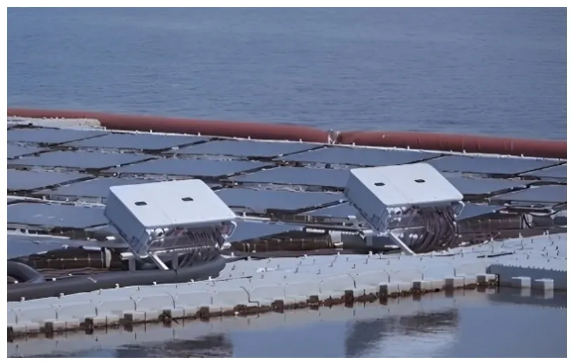
1]. Offshore photovoltaic (PV) power station holds significant development potential due to its minimal reliance on land resources, excellent lighting conditions, and close proximity to power load centers. As a new form of PV power generation, offshore PV has become an important solution to combat the energy transition and climate change. China has built a number of offshore PV demonstration projects in Zhejiang, Jiangsu, Guangdong, Shandong, and other places, and has clearly put forward the strategic goal of vigorously developing offshore PV in the next Five-Year Plan. For example, in July 2022, Shandong Province announced plans to install 42.6 million kilowatts of offshore PV during the 14th Five-Year Plan period [
2].
Compared to land-based PV systems, the design of offshore PV systems is more complex. The design of offshore PV systems encompasses not only the PV arrays, float structures, and anchoring systems, but also power transmission and conversion systems, as well as monitoring and maintenance systems. Due to the unique marine environment, the system must cope with a range of factors, including high temperatures, high humidity, high salinity, lightning strikes, and heavy rainfall. These environmental factors interact and pose significant challenges to the system’s stability and reliability (
).
Figure 1. Offshore PV system.
Within this system, the PV inverter serves as a crucial power conversion device in the system, directly determining the stability and reliability of the entire PV system. Specifically, the DC input side of the PV inverter utilizes a multitude of PV connectors to aggregate the output currents from individual PV modules and integrate them into the electrical system, thereby ensuring efficient conversion and transmission of electrical energy.
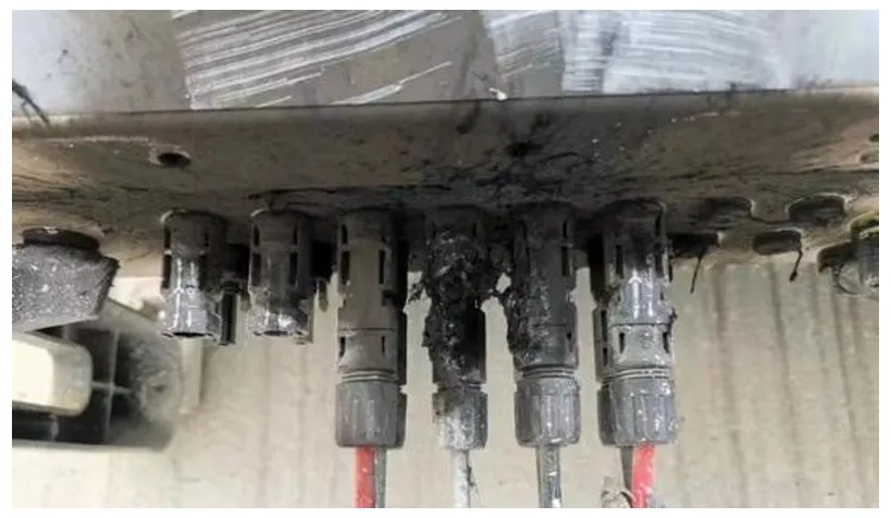
However, long-term exposure of PV connectors to the harsh marine environment, characterized by high humidity, salt spray, and strong corrosion, can significantly increase the contact resistance. This is primarily due to the corrosion and oxidation of the internal metal conductor contact surfaces. Such degradation can lead to thermal effects and even arc fault (
), which pose significant risks to the safety of electrical systems. Therefore, effectively detecting and locating thermal failures in PV connectors has emerged as a key focus and challenge in contemporary research [
3].
Figure 2. Arc fault of PV connectors.
Currently, most thermal fault detection methods for connectors rely primarily on identifying abnormal changes in the temperature field. Common technical means include infrared imaging, thermoelectric sensors, and optical fiber sensing,
etc. [
4]. Among the above-mentioned technical means, infrared temperature measurement is a non-contact measurement. However, due to the complex internal structure of PV inverters, there is a lot of obstruction to the infrared radiation optical path. When used in marine environments, it is highly susceptible to factors such as the temperature, humidity, and solar radiation of the detection environment [
5,
6], which cannot ensure accurate temperature measurement. Moreover, its high cost also limits its application [
7,
8]. Fiber Bragg grating sensors can provide high-precision and high-stability measurements of contacts in environments with high voltage, large currents, and strong magnetic fields, such as those inside switch cabinets. They can easily form a distributed temperature measurement system to conduct real-time online monitoring of all contacts. However, due to the fact that the DC input side of high-power PV inverters is connected to tens or even dozens of PV connectors, this results in a large number of internal measurement parts of the entire PV inverter and high costs [
9,
10]. In contrast, thermoelectric sensing technology, with its advantages of miniaturization, low cost, and high integration, can be well embedded into complex electrical equipment for long-term monitoring. It is the most commonly used means of thermal fault monitoring.
Compared with the research on mature detection technology systems, the studies on the construction of connector thermal models, temperature estimation, and abnormal overheating location are relatively limited, but many scholars have still carried out active explorations. For instance, Li [
11] proposed a thermal fault detection system based on a BP neural network. By establishing a connector temperature field model, the method effectively addresses the issue of excessive temperatures caused by aging or poor contact of busbars and moving/static contacts in high-voltage switch cabinets. K. Zhao et al. [
12] proposed an infrared image recognition algorithm integrating deep learning. This algorithm, through electromagnetic-fluid-thermal coupled numerical calculation and the application of the MASK R-CNN model, can reliably mark and identify each component from the infrared images of gas-insulated switchgear (GIS), accurately calculate their surface temperatures, and further invert the temperature rise of internal connectors, achieving effective detection and location of connector thermal faults in high-voltage and high-current environments. In addition, Wu et al. [
13] constructed a GIS busbar joint temperature prediction model based on the least squares method parameter optimization. They introduced the artificial bee colony algorithm, improved by chaos theory, to optimize the parameters, accurately estimate the busbar joint temperature, and provide reliable support for thermal fault detection and location. However, the above-mentioned studies have all focused on the abnormal overheating detection of a single connector and are not applicable to the scenarios of connector thermal fault detection and location where the number of thermoelectric sensors is limited. Therefore, a key research challenge has long been to establish a thermal model that captures the coupling relationships among connectors and enables precise fault localization with fewer sensors.
To address this issue, this paper refers to the research ideas and technical principles in the field of overheating of lithium-ion batteries [
14,
15] and It proposes a thermal fault location method for connectors of PV inverters based on multiple model estimator (MME). This method combines the lumped thermal model and the abnormal overheating disturbance model, generates state estimation through the parallel Kalman filter, and utilizes the residual probability weighted fusion strategy, significantly improving the accuracy and robustness of thermal fault location in complex environments. At the same time, this paper proposes a deployment scheme for a minimal number of temperature sensors, achieving high-precision thermal fault detection and localization while reducing hardware costs and wiring complexity.
2.1. Theoretical Basis of MME
MME [
16,
17] is a widely used technique for fault detection and location. Under the condition that the mathematical model of the object or disturbance is not completely determined, this technique makes the specified performance index as close to and as optimal as possible by designing the control sequence. The nonlinear problem of estimation control is solved by N linear stochastic control systems. Among them, the multiple model adaptive Kalman filter is an important technical means for dealing with complex control systems.
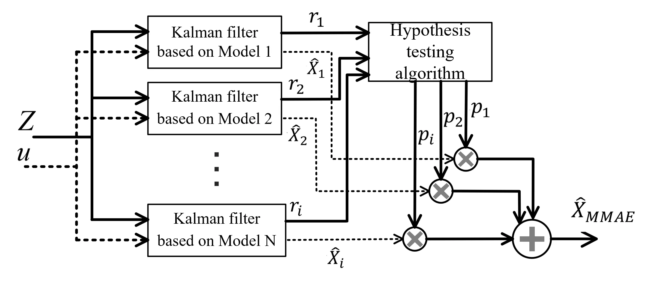
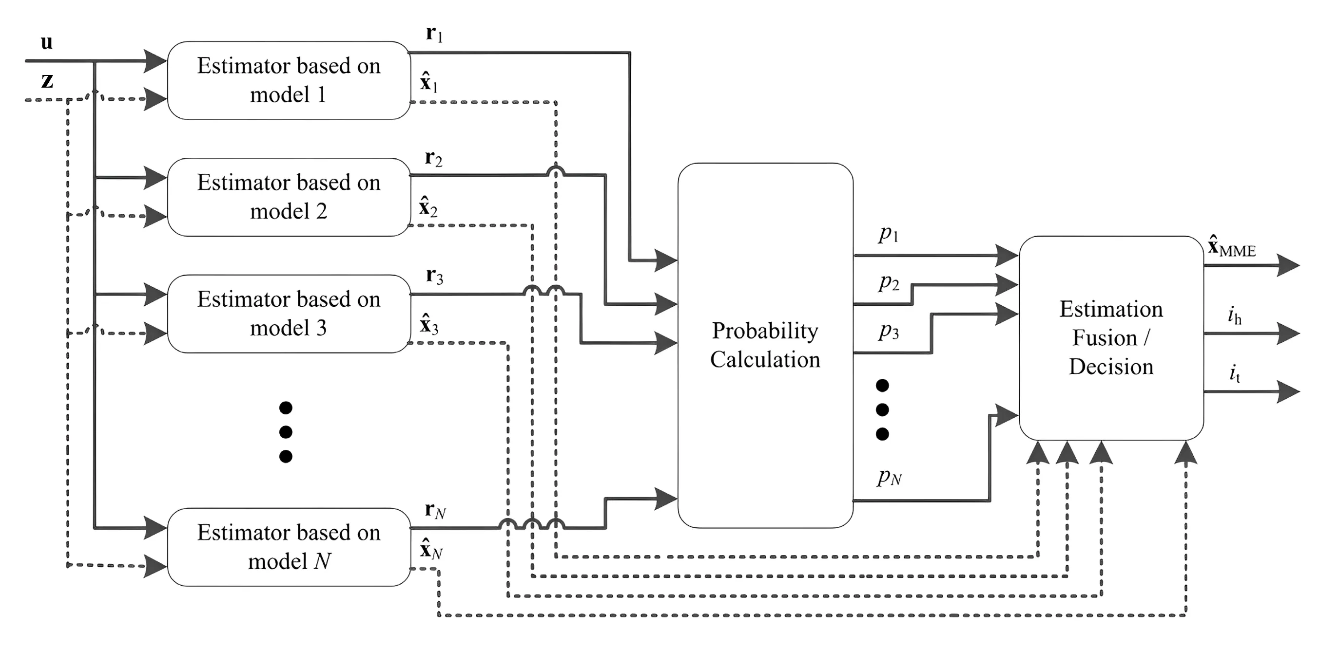
The principle of the multiple model adaptive Kalman filter is shown in
. Each filter model independently calculates the current state estimation of the system $$\hat{X}_{i}$$ based on its built-in model and input vector
u. Then, by calculating the difference from the actual observed vector
Z, the residual $$r_{i}$$ is obtained, which is used as an indicator of the degree of similarity between each filter model and the actual system model. Further, the hypothesis testing algorithm uses the residual to calculate the conditional probability $$p_{i}$$ of each Kalman filter model. Finally, it forms the mixed state estimation of the actual system through the probability-weighted average of each state estimate, so as to ensure the accuracy and robustness of the final state estimation $$\hat{X}_{M M A E}$$.
. Structure diagram of multiple model adaptive Kalman filter.
2.1.1. Multiple Model Adaptive Kalman Filter
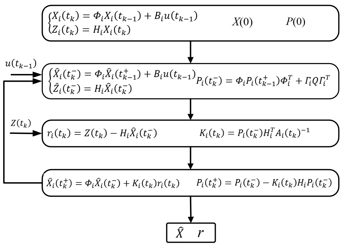
The multiple model adaptive Kalman filter is developed on the basis of the basic Kalman filter equation, which mainly includes the filter model, prediction equation, residual equation, and state update equation.
The Kalman filter model of the system can be expressed as:
where, $$X_{i} $$ and $$Z_{i}$$ are respectively the state vector and measurement vector of the
i-th Kalman filter model,
i = 1, 2, ...,
N; $$\varPhi_{i}$$, $$B_{i}$$, $$\Gamma_{i}$$ and $$H_{i}$$ denote the state transition matrix, control input matrix, noise input matrix, and output matrix of the
i-th Kalman filter model, respectively;
u is the system control input vector; $$w_{i}$$ is the discrete dynamic interference white noise input of the
i-th Kalman filter model and $$v_{i}$$ is the discrete dynamic measurement of white noise for the
i-th Kalman filter model. Where, $$w_{i} $$ and $$v_{i}$$ are unrelated.
The Kalman filter prediction equation of the system can be expressed as:
where, $$\hat{X}_{i}$$ is the state estimation vector of the
i-th Kalman filter; $$\hat{Z}_{i} \left(t_{k}\right)$$ is the prediction of the measured vector by the
i-th Kalman filter before the arrival of time $$t_{k}$$, $$t_{k}^{-} $$ is the moment before the
k-th measurement update; $$t_{k - 1}^{+}$$ is the moment after the (
k − 1)-th measurement update.
The prediction equation of state estimation error covariance matrix can be expressed as:
The state estimation of the Kalman filter is updated by
Equation (4). Here, the gain of the Kalman filter is expressed by
Equation (5), and the residual variance matrix calculated by the Kalman filter is expressed by
Equation (6).
The residual vector of the Kalman filter is the difference between the measured value
Z and the Kalman filter estimate $$H_{i} \hat{X}_{i} \left(t_{k}^{-}\right)$$ based on previous measurements,
i.e.,
The time update equation of the state estimation variance matrix is:
The detailed flow of the Kalman filter algorithm is shown in
.
. Flowchart of Kalman filter algorithm.
2.1.2. Probabilistic Fusion
The hypothesis testing algorithm is used to evaluate and confirm various hypotheses. It checks the residuals of all Kalman filters in the model estimator. If the model of a filter matches the real model of the system, then the residual will be presented as a Gaussian random noise sequence with zero mean, whose variance is:
Under the condition of the measured value $$Z^{t_{k-1}}=[Z^T(t_1),\cdots,Z^T(t_{k-1})]^T$$, and the model parameter vector $$a \in \{a_1,a_2,\cdots,a_k\}$$, the conditional probability density function of the measured value $$Z \left(t_{k}\right)$$ of the
i-th Kalman filter model at time $$t_{k}$$ is:
In the equation:
$$\left\{\cdot\right\} = \left\{- \frac{1}{2} r_{i}^{T} \left(t_{k}\right) A_{i}^{- 1} r_{i} \left(t_{k}\right)\right\} , \beta_{i} = \frac{1}{\left(2 \pi\right)^{m / 2} \left|A_{i}\right|^{1 / 2}}$$,
m is the measurement vector dimension.
The conditional probability of a Kalman filter model can be defined as:
Then the conditional probability of the Kalman filter model can be expressed as:
By assuming the conditional probability of the model, the weighted fusion of state estimates of different Kalman filter models is realized, and the mixed state estimate $$\hat{X}_{M M A E}$$ of the real system is obtained:
If the correct model is included in the estimator, then the model probability of the correct model converges to 1. Otherwise, the probability value of the model closest to the real model converges to 1.
2.2. PV Connector Lumped Thermal Model
2.2.1. Single PV Connector Thermal Model
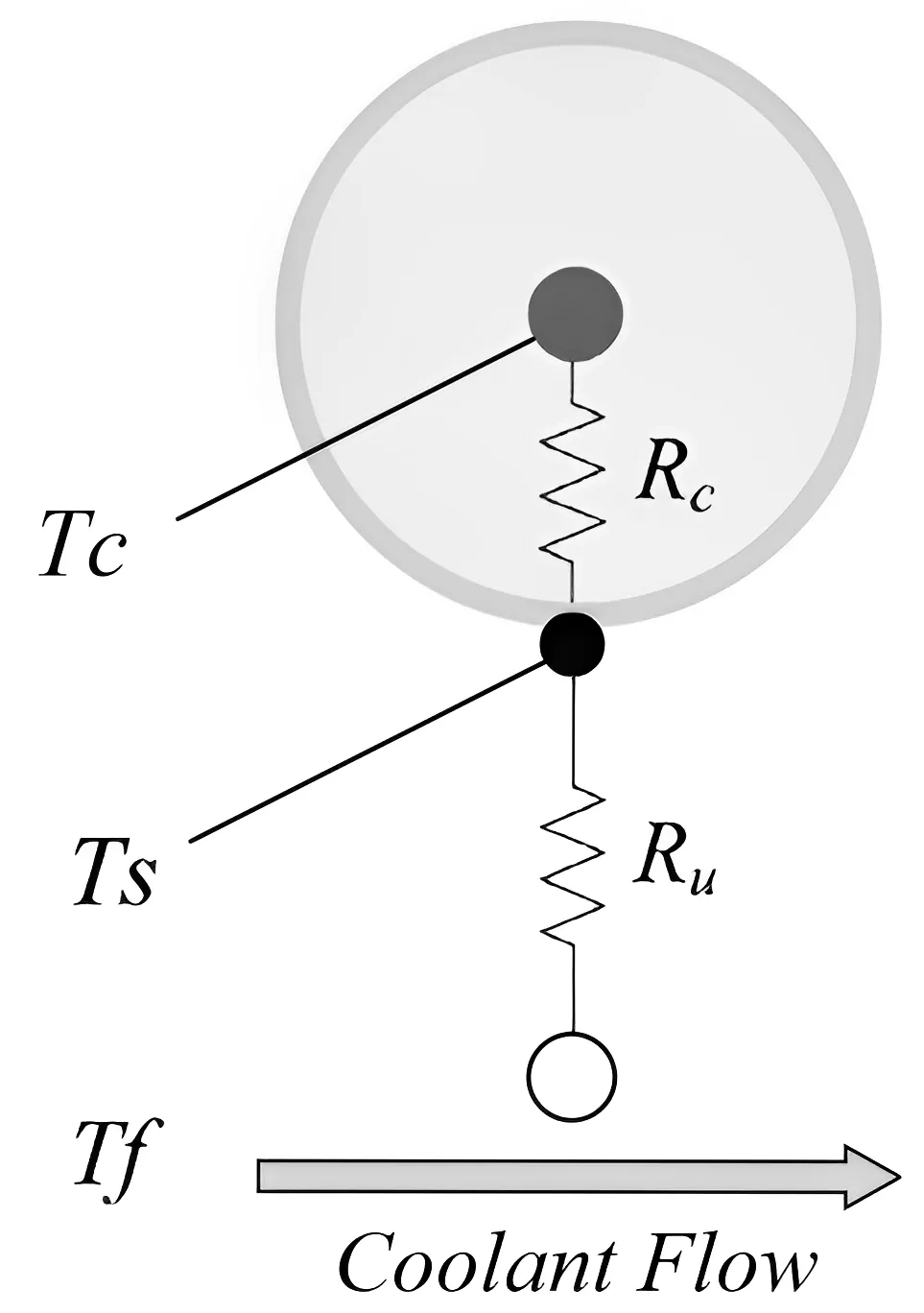
In order to study the heating characteristics of PV connectors, the thermal model of a single connector is established here, and its structure is shown in
. In order to facilitate analysis and calculation, the geometric characteristics of the actual connector are reasonably simplified, and the shape of the model is assumed to be an ideal cylinder. The temperature state of the cylindrical PV connector is modeled at two levels, one is the shell temperature
Ts, and the other is the temperature
Tc of the internal metal core.
. Lumped heat model of a single PV connector.
The thermal model of the above single PV connector can be expressed as follows:
In this model, based on the simplified structure, the heat generation is approximately the joule loss caused by heating the metal core inside the connector, calculated as the product of the square of the current
I and the internal resistance
Re. Generally,
Re depends on both temperature and material properties, and other factors, in order to facilitate the study, the
Re of the normal working PV connector is set as a constant, and the default does not change with temperature or material properties. At the same time, the temperature distribution of the inner metal core and shell is assumed to be uniform.
In order to accurately reflect the internal heat transfer mechanism, the modeling of the heat exchange process is simplified in this study. In it, the heat exchange between the metal core and the surface is simulated by heat conduction over the thermal resistance
Rc, which is a lumped parameter that includes both conduction and contact thermal resistance.
Ru represents the resistance of heat convection between the surface and the surrounding air, and is used to consider air convection. The air temperature is denoted as
Tf.
Cc represents the heat capacity of the metal core inside the PV connector, and
Cs is the heat capacity of the connector shell.
2.2.2. Multi-Connector Lumped Thermal Model
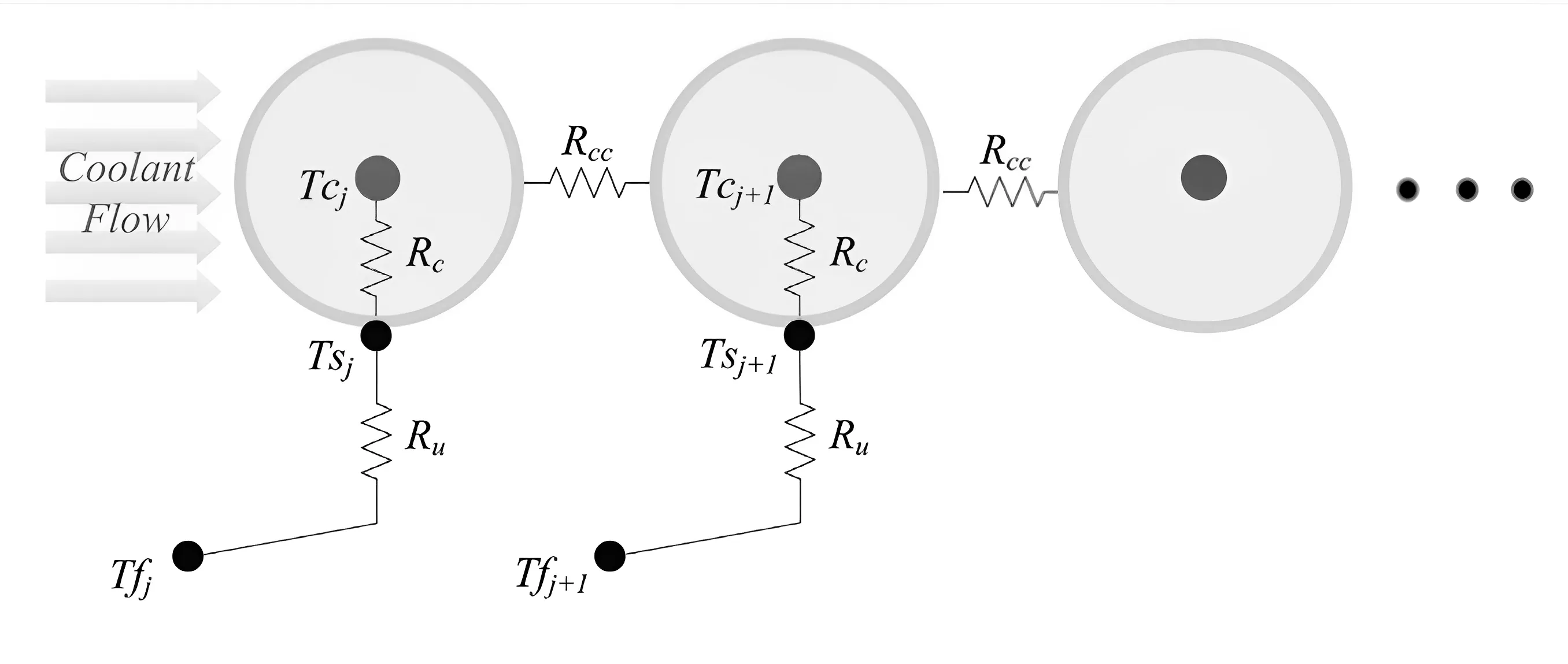
The lumped thermal model of several adjacent PV connectors arranged equidistantly is shown in . The model consists of N single connectors.
. Lumped thermal model of N connectors.
Based on the lumped thermal model of a single connector, a general law applicable to the thermal model of N connectors can be summarized, that is, considering a system composed of N PV connectors, the heat equation of the
j-th PV connector can be expressed as:
In the equation,
Tsj is the temperature of the connector shell,
Tcj is the temperature of the metal core inside the PV connector,
Rc is the equivalent thermal resistance of the internal metal core to the surface of the shell, and
Ru is the thermal resistance of the surface of the shell to the air.
Cc is the heat capacity of the metal core inside the connector, and
Cs is the heat capacity of the connector housing.
Tf is the ambient air temperature.
Rcc is a lumped parameter that includes the conduction and contact thermal resistance of adjacent PV connectors connected by a metal substrate.
Cf is the heat capacity of air.
2.2.3. System State Equation
Although the number of PV connectors is not limited by a specific limit, in order to simplify the analysis, this paper takes six PV connectors (that is,
N = 6) arranged at equal distances as the research object.
By rewriting
Equation (16) and
Equation (17), a set of state observation equations in the form of a matrix of PV connectors thermal model system can be obtained:
For a thermal model system with
N = 6:
In the above equation,
A and
B are the system matrices, and
C is the output matrix. The measurement of the state is expressed as 1 in the output matrix
C. For example, a thermal model with two PV connectors has four temperature states, namely
Tc1,
Ts1,
Tc2 and
Ts2. Measuring the metal core temperature of PV connector 1 can be expressed as a
C matrix with a value of [1 0 0 0]. From the
A and
C matrices of the system, the observability of the system can be checked and further become the basis for determining the minimum number of temperature sensors in a set of PV connectors thermal model [
14,
18].
2.3. Modeling of Abnormal Overheating Disturbance
Considering the Joule heat increment caused by increasing contact resistance as an unknown input disturbance, state and interference estimation based on Kalman filter is established.
2.3.1. Unknown Disturbance Hypothesis
According to
Equation (16), the heat generated inside the PV connector and the heat released jointly determine the thermal balance state of the metal core. During abnormal overheating caused by increased contact resistance, the energy balance of the PV connector metal core can be described by the following equation:
In the equation,
Qr is the Joule heat in the abnormally overheating state (
i.e.,
I2R term), and
Qrelease is the heat released to the outside of the metal core (
i.e., $$\frac{T_{c} - T_{s}}{R_{c}}$$ term in
Equation (16)).
For a PV connector model that causes abnormal overheating due to increased contact resistance, the Joule heating term represents the additional energy released by the increased contact resistance. At this time, the resistance
R of the
I2R term in
Equation (16) changes. Since the original thermal model did not account for this additional Joule term, this “additional” term can be regarded as an unknown disturbance in the system.
2.3.2. Unknown Disturbance Modeling
In a control system, the system is usually augmented by introducing an integrator driven by white noise to effectively deal with unknown disturbances that cause steady-state migration [
19,
20].
Let a linear, time-invariant discrete-time system have the form shown in
Equation (25), which is augmented by
Equation (26).
In
Equation (25) and
Equation (26), $$\mathbf{x} \left(k\right) \in R^{n}$$ is the state vector of the system at time k, $$\mathbf{u} \left(k\right) \in R^{m}$$ is the input vector, $$\mathbf{z} \left(k\right) \in R^{p}$$ is the measurement vector, and $$\mathbf{d} \left(k\right) \in R^{n d}$$ is the interference vector. The perturbation acts on the state through the matrix $$\mathbf{B}_{d} \in R^{n \times n d}$$ and on the measurement through the matrix $$\mathbf{C}_{d} \in R^{p \times n d}$$. By setting $$\mathbf{C}_{d}$$ to zero, a pure input perturbation model can be obtained. By setting $$\mathbf{B}_{d}$$ to zero, a pure output perturbation model can be obtained.
Next, you need to verify the detectability of the augmentation system. This step is critical because augmentation systems must be detectable. According to [
19,
20], the detectability of augmentation systems can be verified by the following conditions:
2.3.3. State and Interference Estimation Based on Kalman Filter
After adding additional unknown interference vectors to the original system, a steady-state Kalman filter is designed to estimate the state and interference of the system. Suppose that the model in
Equation (26) is expanded to include a zero-mean white noise process term $$\mathbf{w} \left(k\right)$$ and a zero-mean white noise measure term $$\mathbf{v} \left(k\right)$$, in the following form:
Let the covariances of $$\mathbf{w} \left(k\right)$$ and $$\mathbf{v} \left(k\right)$$ be $$\bm{Q}_{\bm{w}}$$ and
R, respectively, and $$\mathbf{w} \left(k\right)$$ and $$\mathbf{v} \left(k\right)$$ are not correlated. $$\mathbf{G}$$ is the noise gain matrix, the process noise is associated with the state variable, and $$\mathbf{G} = \mathbf{I}$$ is selected. The interference is driven by white noise $$\xi \left(k\right)$$ and its covariance is $$\bm{Q}_{\xi}$$.
The state and disturbance of the system are first predicted by the Kalman filter, and then the output $$\mathbf{z} \left(k\right)$$ is used to update the state and disturbance of the system, in the following form:
2.4. Design of MME
2.4.1. Parallel Estimator Design
In the case described in Section 2.3, the augmented system and estimator are designed to handle interference that affects only one particular PV connector. However, if the interference affects other PV connectors, new augmentation systems and estimators need to be designed accordingly.
shows the operation of N parallel estimators, each based on the same system model and assuming that interference affects only one of the cells at a time. Each estimator model is represented by the parameter
ai, where
i = 1, 2, ..., N. Based on the input
u and output
z, these estimators generate state estimates, such as
Equation (31) and
Equation (32).
. Working principle diagram of N parallel estimators.
2.4.2. Probability Calculation and Estimation Fusion
In order to determine which unit is affected by the interference, the conditional probability $$p_{i} \left(k\right)$$ is defined, that is, the probability that
a is
ai (
i.e., assuming that the
i-th model is the real model) after observing the measurement history to the time step
k. This means that by calculating the conditional probability for each model, the system can determine which unit is most likely to be disturbed and give an estimate accordingly.
The conditional probability is shown as follows:
In the equation, $$\mathbf{Z} \left(k - 1\right) = \left[\mathbf{z}^{T} (1) \ldots \mathbf{z}^{T} \left(k - 1\right)\right]^{T}$$.
At the same time, $$p_{i} \left(k\right)$$ can be iteratively updated by recursively evaluating all
i to:
where $$f_{\mathbf{z} \left(k\right) \left|\right. a , \mathbf{Z} \left(k - 1\right)} \left(\mathbf{z}_{k} \left|\right. a_{i} , \mathbf{Z}_{k - 1}\right)$$ is the conditional density function of measuring
z with time step
k given a certain Kalman filter model $$a\in\{a_{1,},a_2,\ldots,a_N\}$$ and measurement history $$\mathbf{Z}_{k - 1}$$. The conditional density function is defined as:
From Equations (33) to (34), it can be seen that if the interference affects a specific state quantity (
i.e., a PV connector unit), then the corresponding estimator model ai will produce a smaller residual than the other models. Therefore, the model is more likely to be the one that best matches the actual system.
Similar to the method in [
21], the estimated fusion/decision module selects the model index $$i_{h} \left(k\right)$$ with the highest probability at each time step k through decision logic, and its calculation method is as follows:
The final determination of the real model index $$i_{t} \left(k\right)$$ is done by using the probability threshold $$p_{t h r e s h}$$, which is expressed as:
Therefore, the real model index $$i_t (k)$$ identifies abnormally overheating PV connectors.
In this paper, the probability threshold $$p_{t h r e s h} = 0 . 75 $$ is selected as the criterion to determine the real model according to the results of multiple simulations. Because once the probability predicted by the model reaches this threshold, the model can be judged as the final true model.
Based on the design of PV connector thermal model and MME constructed in Section 2, this chapter further researches the thermal fault location of PV connectors. Based on the clustering model, the observability of the system is analyzed, and the precise location of abnormally overheating PV connectors is discussed under the condition of minimum sensor configuration.
3.1. Sensor Deployment Based on the Observability of Clustering Models
An effective closed-loop observer is based on the observability of the model. In this section, observability conditions are analyzed to guide the placement of sensors in a particular cell in a set of PV connector units, enabling effective temperature detection.
Observability of the thermal model of the PV connector described above can be tested by
Equation (39):
where,
A is the system matrix,
C is the output matrix in
Equation (27), and n is the system order. The model is fully observable if and only if the rank of
Q is equal to n [
14].
For a thermal model that contains two PV connector units, the system matrix A is expressed as
Equation (40).
The matrix
C will be determined by the position of the temperature sensor. If the temperature sensor measures the temperature of the metal core of PV connector #1,
C1 = [1 0 0 0]; If the sensor is measuring the metal core temperature of PV connector #2, then
C2 = [0 0 1 0].
If we assign all the elements of the set
A to the values in this article and compute
Q by substituting them into the
Equation (39), we find that the rank of the matrix
Q is 4 when either
C1 or
C2 is used. This means that full observability can be achieved for a set of PV connectors consisting of two units, regardless of whether the first or second unit is measured.
Similarly, for
A thermal model of any number of PV connector units, after establishing the system matrix A, an observability analysis can be performed to determine the minimum number of sensors to achieve full observability. The observability test of system matrix
A can be specifically referred to [
14], and the relevant results are summarized as shown in
.
.
Minimum number of sensors for different connector units to achieve full observability conditions.
| Number of Units |
Minimum Number of Sensors |
| 1,2,3 |
1 |
| 4,5,6 |
2 |
| 7,8,9 |
3 |
| 10,11,12 |
4 |
3.2. Thermal Fault Location Simulation and Analysis
In this paper, MATLAB is used to locate the abnormal overheating fault of 6 PV connector models arranged in adjacent equidistant.
3.2.1. Conditional Input
Assume that one of the six PV connector units has an overheating disturbance. As described in Section 2.3, to account for heat generation in real systems, an unknown input $$\mathbf{p}$$ is introduced into the continuous time state-space model with the following expression:
In
Equation (41), the matrices $$\mathbf{B}_{p c}$$ and $$\mathbf{p}$$ can be viewed as additional generated heat. For example, in
Equation (42), the sixth connector is abnormally overheated (that is, an additional
Qrc term is added to the original state quantity
Tc6).
In the previous section, it was explained that when the number of PV connector units in a set is 6, the minimum number of sensors required to meet the condition of full observability is 2. Now, assume that the temperature sensor is configured on the third and sixth PV connectors. The system equation
C can be expressed as:
In this paper, it is assumed that the initial temperature of the 6-unit PV connector is the same as the ambient temperature, which is 25 ℃. Considering the influence of air convection, the airflow direction is from left to right, and the
Ru value corresponding to the gas flow is 0.6 × 10⁻³ m³/s. In addition, the rated channel current of the PV connector is set to 20 A, and the contact impedance is maintained at a constant value
Re = 0.25 mΩ.
It is assumed that due to the corrosion of the metal core contact surface, the contact impedance of the connector is abnormally increased, which causes abnormal overheating behavior of a connector unit (denoted as
Qr). Specifically, the heat input
Qr of abnormal overheating behavior is set to 5 W and 3 W, respectively, and the selection of relevant parameters is based on the study on abnormal overheating resistance of PV connectors in [
22,
23]. The heat input is applied from t = 0 s until the PV connectors reach the steady-state operating temperature, aiming to simulate the abnormal overheating behavior under different heating power, and to compare and analyze the temperature change characteristics under the two working conditions.
The specific parameters of the thermal model are shown in
. The materials and parameters in the table are determined according to [
24,
25] and the PV connector test methods and requirements in the international standard IEC 62852:2020.
.
Specific materials and working parameters of the thermal model.
| Argument |
Numerical Value |
Argument |
Numerical Value |
| Irated |
20 A |
Re |
0.25 mΩ |
| Cc |
1.16 JK−1 |
Cs |
19.8 JK−1 |
| Rc |
5.42 KW−1 |
Rcc |
2.81 KW−1 |
3.2.2. Comparison of Simulation Results
Considering a 6-unit connector thermal model with only two temperature sensors, the following two scenarios are analyzed. In the first case, the abnormally overheated connector is a connector with a temperature sensor, and in the second case, the abnormally overheated connector is a connector without a temperature sensor. The results show how the probabilities of each augmentation model evolve over time, as well as the resulting state estimates for the dominant (highest) probability model.
- (1)
-
Abnormally overheated PV connectors containing temperature sensors
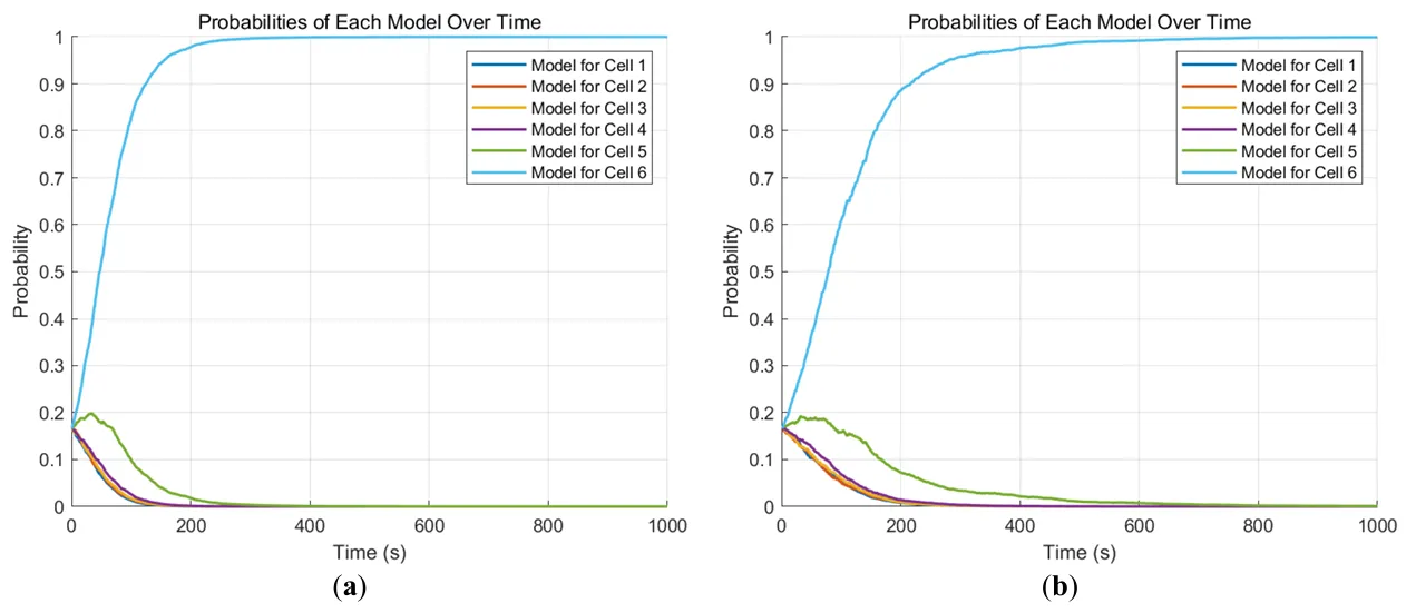
① Abnormal overheating is detected in the PV connector #6.
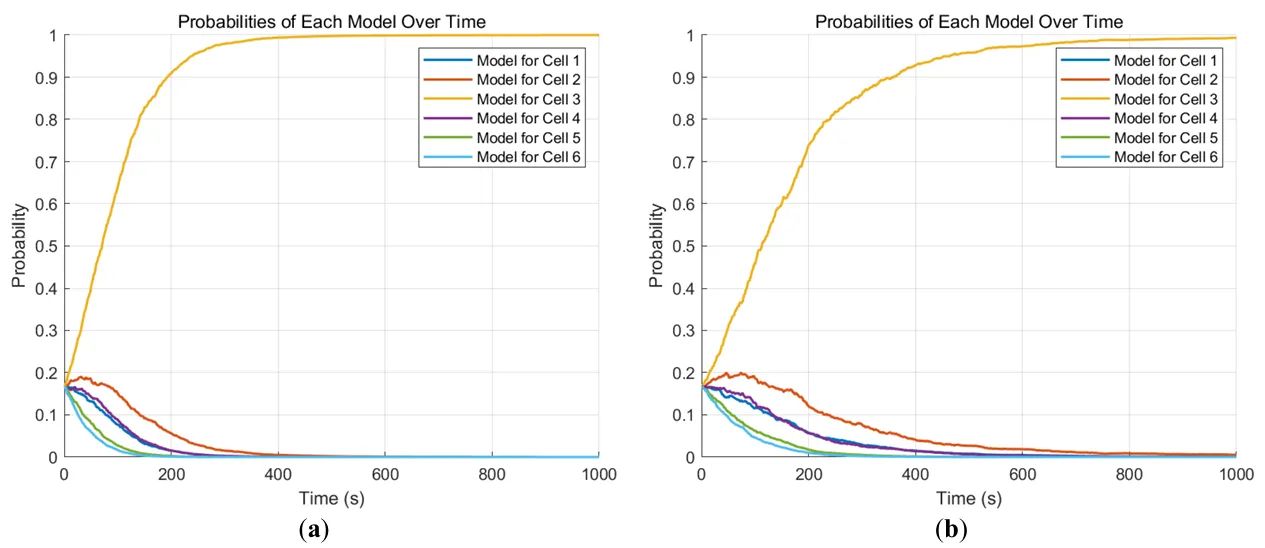
shows the probability $$p_{i} \left(k\right)$$ of each of the six augmentation models used by the estimated decision block to identify
Equation (37). It can be seen that when the PV connector #6 introduces interference at t = 0 s, the probability of the real model corresponding to the augmented model 6 gradually increases to 1 over time, while the probability of the other models gradually approaches 0.
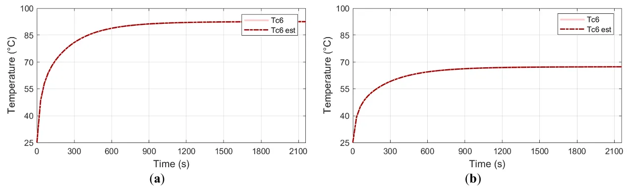
Each augmentation model has the same probability before the perturbation enters. The temperature is estimated according to the dominant (highest) probability model. When the heating power of the PV connector #6 is 5 W, the system determines the real model at t = 78 s. When the abnormal heating power is 3 W, the time for the system to judge the real model is extended to t = 140 s. In addition,
shows the MME estimated temperature of the PV connector #6 abnormally overheated PV connector model compared to the true temperature.
. Probability of the six augmented models when the PV connector #6 is abnormally overheated, (<b>a</b>) 5 W heating power; (<b>b</b>) 3 W heating power.
. Comparison between the actual temperature of PV connector # 6 and the estimated temperature of MME, (<b>a</b>) 5 W heating power; (<b>b</b>) 3 W heating power.
② Abnormal overheating is detected in PV connector #3.
shows the probability $$p_{i} \left(k\right)$$ used to estimate the decision block for each of the six augmenting models of the identification
Equation (37) when the PV connector #3 is abnormally overheated.
. Probability of the six augmented models when the PV connector #3 is abnormally overheated, (<b>a</b>) 5 W heating power; (<b>b</b>) 3 W heating power.
- (2)
-
Abnormally overheated PV connector without temperature sensor
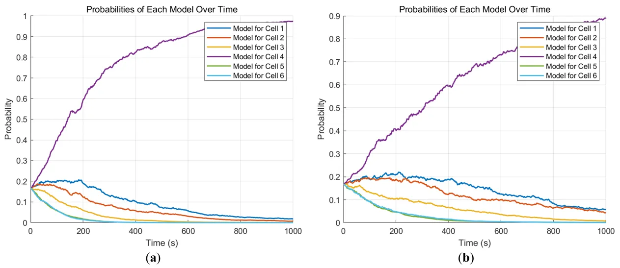
As can be predicted from the previous discussion, if abnormal overheating occurs in any of the PV connectors where the temperature is not measured, it may take longer, since each increase in interference affects only one of the PV connector units until the nearest sensor senses the temperature anomaly. The following shows the results of the overheating of PV connector #4. In
, the
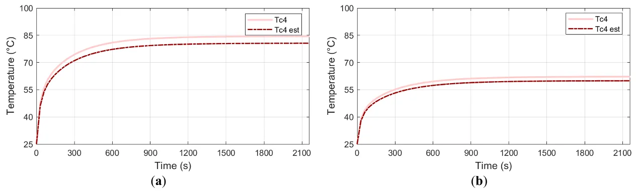
p4 value exceeds the probability threshold of 0.75 at t = 302 s (5 W) and at t = 470 s (3 W), respectively. In
, the red solid line represents the measured temperature, and the red dashed line represents the MME estimated temperature.The evolution of the probability of other abnormal overheating conditions is shown in
(PV Connector #2),
(PV connector #5), and
(PV connector #1). It can be noted that the MME takes quite a long time to determine the model of abnormal overheating.
① Abnormal overheating is detected in PV connector #4.
shows the probability $$p_{i} \left(k\right)$$ used to estimate the decision block for each of the six augmentation models of the identification
Equation (37) when the PV connector #4 is abnormally overheated.
shows the comparison between the actual temperature of the PV connector #4 model and the estimated temperature of the MME.
. Probability of six augmented models when the PV connector # 4 is abnormally overheated, (<b>a</b>) 5 W heating power; (<b>b</b>) 3 W heating power.
Figure 12. Comparison between the actual temperature of PV connector # 4 and the estimated temperature of MME, (<b>a</b>) 5 W heating power; (<b>b</b>) 3 W heating power.
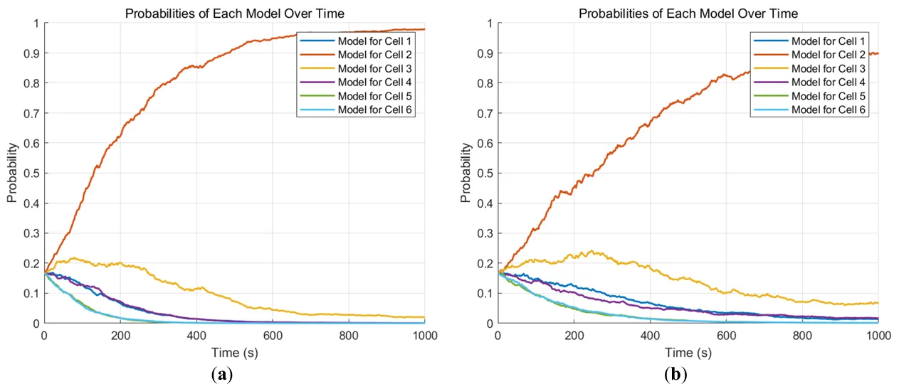
② Abnormal overheating is detected in the PV connector #2.
shows the probability $$p_{i} \left(k\right)$$ used to estimate the decision block for each of the six augmented models of the identification
Equation (37) when the PV connector #2 is abnormally overheated.
. Probability of the six augmented models when the PV connector # 2 is abnormally overheated, (<b>a</b>) 5 W heating power; (<b>b</b>) 3 W heating power.
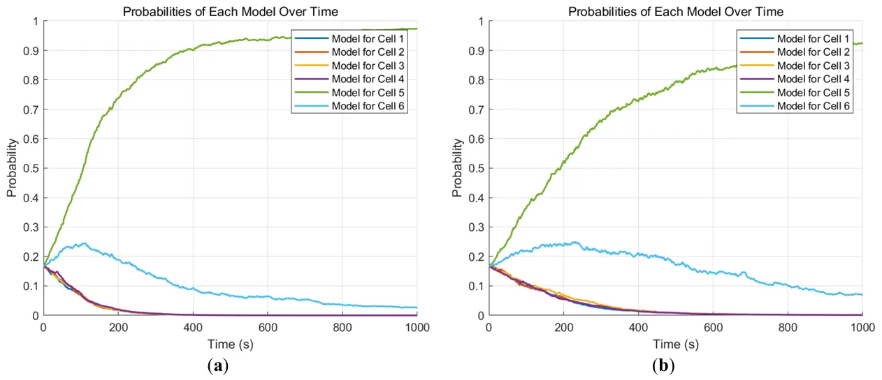
③ When the PV connector #5 is abnormally overheated.
shows the probability $$p_{i} \left(k\right)$$ used to estimate the decision block for each of the six augmented models of the identification
Equation (37) when the PV connector # 5 is abnormally overheated.
. Probability of the six augmented models when the PV connector #5 is abnormally overheated, (<b>a</b>) 5 W heating power; (<b>b</b>) 3 W heating power.
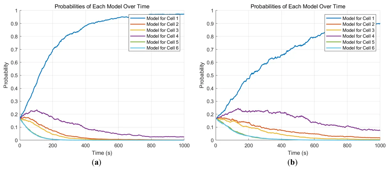
④ Abnormal overheating is detected in PV connector #1.
When the PV connector #1 is abnormally overheated,
shows the probability $$p_{i} \left(k\right)$$ used to estimate the decision block for each of the six augmented models of the identification
Equation (37).
. Probability of the six augmented models when the PV connector #1 is abnormally overheated, (<b>a</b>) 5 W heating power; (<b>b</b>) 3 W heating power.
3.2.3. Determine the Actual Model Timing
summarizes the time taken to locate the real model (
i.e., abnormally overheated model) based on temperature sensors in the PV connector #3 and #6. It can be seen that the higher the heating power, the shorter the fault location time, and vice versa.
.
Time to locate an abnormally overheated PV connector.
| Abnormally Overheated PV Connector |
Time to Locate the Overheating PV Connector |
| Heating Power 5 W |
Heating Power 3 W |
| PV Connector #1 |
243 s |
549 s |
| PV Connector #2 |
287 s |
504 s |
| PV Connector #3 |
127 s |
211 s |
| PV Connector #4 |
302 s |
470 s |
| PV Connector #5 |
212 s |
425 s |
| PV Connector #6 |
78 s |
140 s |
3.3. Experimental Validation
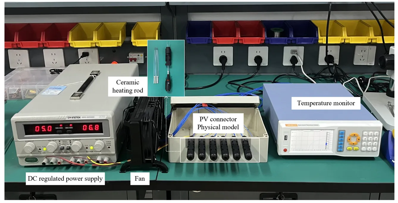
3.3.1. Experimental System
The experimental system consists of a DC power supply, a temperature monitor, and six PV connectors arranged at equal distances. Ceramic heating rods are used to simulate abnormal heating.
The experiment was carried out at a constant ambient temperature of 25 ℃. The heating power of the analog abnormal heating connector is set to 5 W, and the heating power of the other PV connectors is 0.1 W. The temperature sensor is arranged at the connection gap of the PV connector #6, and the metal core of the abnormally overheated PV connector.
Before the experiment, the resistance value of the ceramic heating rod is measured, and the output voltage of the DC voltage regulator is calculated and adjusted according to the resistance value, so that the voltage at both ends reaches the set value. The temperature data was then recorded at a rate of once per second with a duration of 3600 s using a temperature monitor. A total of three experiments were conducted, and the average value was taken as the final experimental data.
is the experimental measurement site, and the relevant experimental parameters are set as shown in
.
.
Settings of relevant experimental parameters.
| Ambient Temperature |
Normal PV Connectors |
Abnormal PV Connectors |
Data Recording Duration |
| 25 ℃ |
0.1 W |
5 W |
3600 s |
3.3.2. Experimental Result
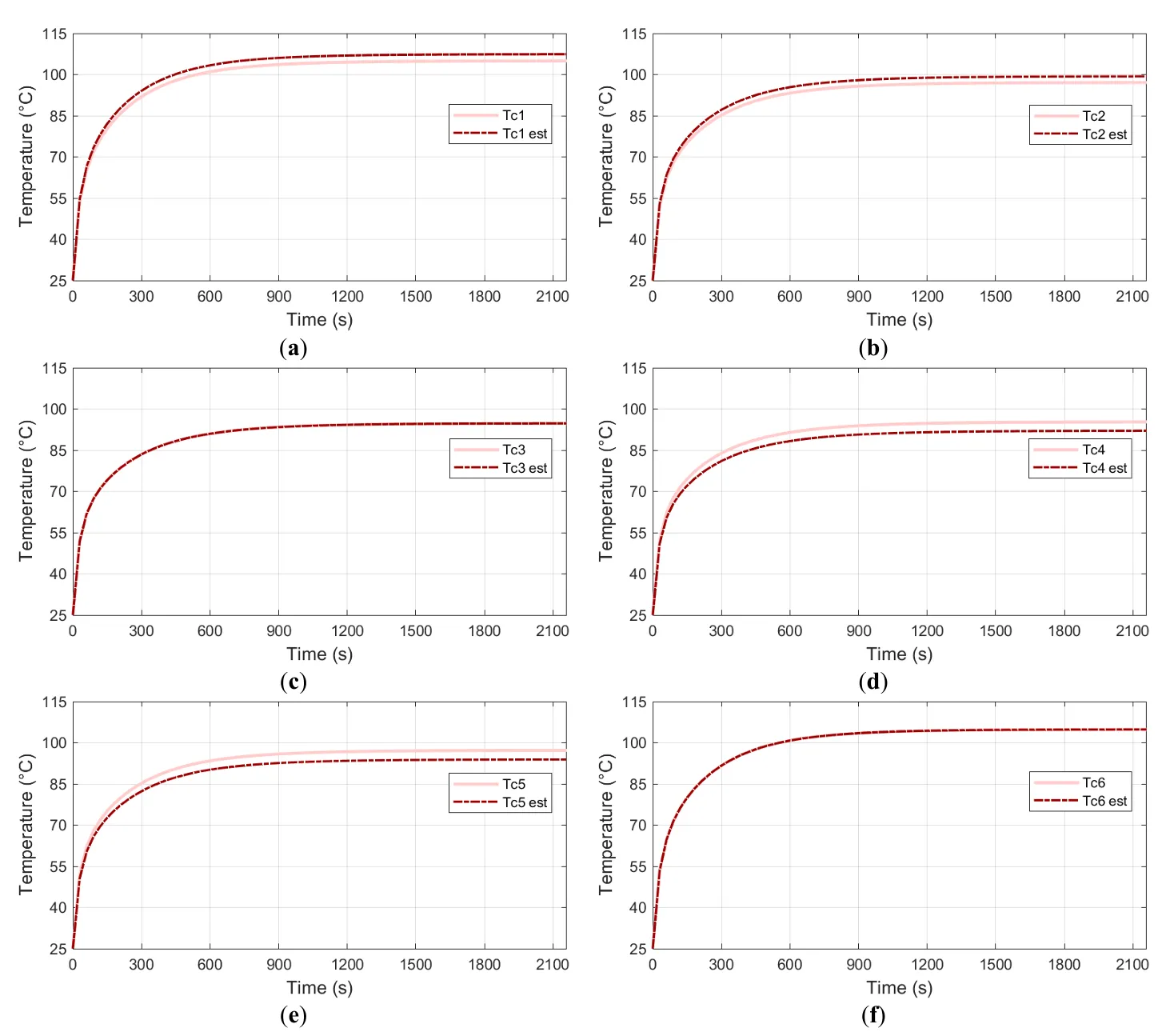
The comparison between MME estimated temperature and measured sensor data is shown in
. In addition, the specific values after reaching the steady state are shown in
.
. MME estimated temperature and actual measured temperature in the case of abnormal overheating of each PV connector. (<b>a</b>) PV connector #1; (<b>b</b>) PV connector #2; (<b>c</b>) PV connector #3; (<b>d</b>) PV connector #4; (<b>e</b>) PV connector #5; (<b>f</b>) PV connector #6.
.
Comparison of the specific values after steady state.
| Abnormally Overheated PV Connector |
Simulation Temperature |
Measured Temperature |
| PV Connector #1 |
107.4 ℃ |
104.9 ℃ |
| PV Connector #2 |
99.3 ℃ |
97.1 ℃ |
| PV Connector #3 |
94.7 ℃ |
94.7 ℃ |
| PV Connector #4 |
92.0 ℃ |
95.3 ℃ |
| PV Connector #5 |
93.8 ℃ |
97.2 ℃ |
| PV Connector #6 |
104.7 ℃ |
104.7 ℃ |
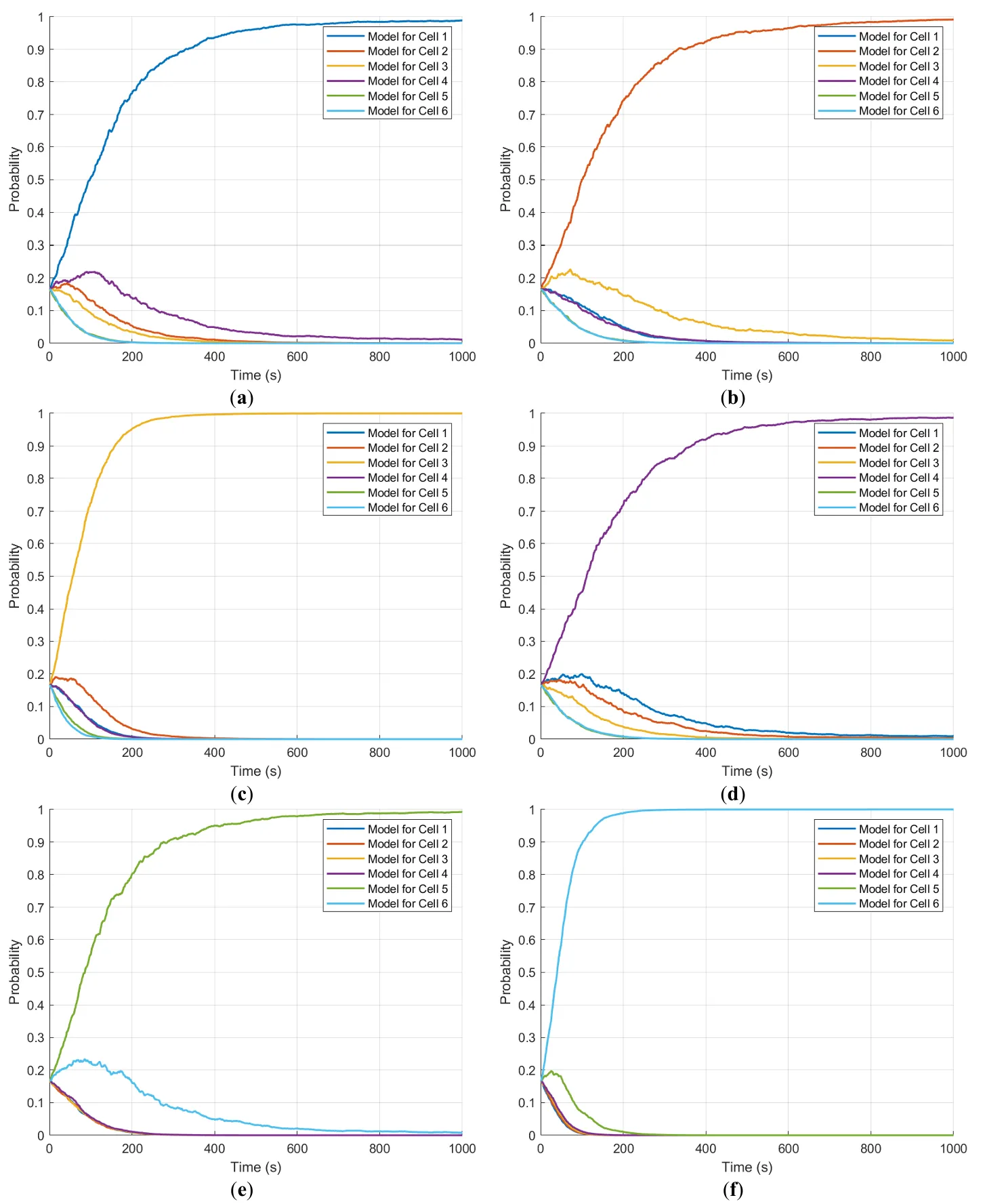
The probability evolution of the obtained models is shown in
.
. Augmentation probabilities of the six models in the case of abnormal overheating of each connector. (<b>a</b>) PV connector #1; (<b>b</b>) PV connector #2; (<b>c</b>) PV connector #3; (<b>d</b>) PV connector #4; (<b>e</b>) PV connector #5; (<b>f</b>) PV connector #6.
Combined with the analysis of simulation results, the measured temperature data of #3 and #6 temperature sensors show a high trend. This bias may result from idealized assumptions of the model, such as the assumption that the temperature distribution of the shell and metal core is uniform during model definition, or some non-ideal factors in the experimental setup are not fully taken into account.
However, analyzing the model probability of each connector in the case of abnormal overheating is a good fit with the simulation results. This proves that the proposed MME algorithm can accurately identify and locate abnormally overheated PV connectors.
This paper presents a novel thermal fault detection and location methodology utilizing MME to address the issue of abnormal overheating in PV connectors on the DC input side of PV inverters in offshore PV systems. By constructing the lumped thermal model and abnormal overheating disturbance model of PV connectors, combined with the multiple model adaptive Kalman filter algorithm, the thermal fault detection and accurate location are realized by using the minimum temperature sensor. Simulation results demonstrate that the proposed method effectively identifies faults under varying heating power levels, significantly reducing localization time as power increases (e.g., the fastest 78 s at 5 W). The experimental validation further confirms the algorithm’s proficiency in accurately identifying abnormally elevated PV connectors, with the experimental data exhibiting a strong alignment with the simulation results.
We extend our sincere gratitude to all members of Tianjin Key Laboratory of New Energy Power Conversion, Transmission and Intelligent Control for their support of this research.
Conceptualization, C.W. and L.Z.; Methodology, L.Z.; Software, L.Z.; Validation, C.W., L.Z. and P.C.; Formal Analysis, L.Z.; Investigation, L.Z.; Resources, C.W. and P.C.; Data Curation, L.Z.; Writing—Original Draft Preparation, C.W. and L.Z.; Writing—Review & Editing, C.W., L.Z. and Q.X.; Visualization, C.W. and L.Z.; Supervision, C.W. and P.C.; Project Administration, C.W., L.Z., P.C. and Q.X.; Funding Acquisition, C.W. and P.C.
Not applicable.
Not applicable.
The statement is required for all original articles which informs readers about the accessibility of research data linked to a paper and outlines the terms under which the data can be obtained.
This paper was partially supported by the National Key R&D Program of China (No. 2022YFB4200703).
The authors declare that they have no known competing financial interests or personal relationships that could have appeared to influence the work reported in this paper.