1. Introduction
The 6-DOF bicopter is a type of aerial drone that is widely used in civilian and defence applications [
1,
2,
3]. The dynamic model of the 6-DOF bicopter is characterized by complex nonlinearities and underactuation [
4,
5,
6]. Such UAVs combine the advantages of vertically take-off and landing drones with the high speed of fixed-wing rotorcrafts. To describe the position and the velocity of the 6-DOF bicopter an inertial and a body-fixed reference frame is defined [
7,
8,
9]. These frames are connected with rotation matrices. Typically, the state-space description of this aerial drone comprises 12 state variables out of which the first six are the cartesian coordinates of the drone and its orientation (Euler) angles for rotation around the axis of the inertial reference frame [
10,
11,
12]. The rest of the state variables of this UAV are the linear velocities that describe the translational motion of the drone in the inertial reference frame and the angular velocities which describe the turn speed of the drone around the axes of the inertial reference frame [
13,
14,
15]. So far, several nonlinear control methods have been proposed for the stabilization and autonomous navigation problem of the 6-DOF bicopter [
16,
17,
18]. Some of these methods consider simplified linear models of the bicopter while others attempt the inversion of this drone’s dynamics [
19,
20,
21]. Adaptive and robust control schemes have been also proposed [
22,
23,
24]. Due to the complexity of the nonlinear dynamic model of the 6-DOF bicopter and because of underactuation the nonlinear optimal control problem for the 6-DOF bicopter has been little dealt with up to now. The autonomous navigation problem of tandem rotor helicopters is also a relevant topic where control methods for bicopters can be applied [
25,
26,
27,
28,
29].
In this article nonlinear optimal (H-infinity) control is proposed for the dynamic model of the 6-DOF bicopter [
30,
31,
32]. By proving first differential flatness properties for this UAV, the nonlinear controllability of the dynamics of the 6-DOF bicopter is confirmed [
33,
34]. To apply the nonlinear optimal control method, the dynamic model of the bicopter is linearized sequentially (at each sampling instance) around a time-varying operating point that is also updated at each sampling interval. This linearization point $$(x^∗,u^∗)$$ is defined by the present value of the system’s state vector $$u^{∗}$$ and by the last sampled value of the control inputs vector $$u^{∗}$$. The linearization is based on Taylor series expansion and on the computation of Jacobian matrices [
35,
36,
37,
38]. For the linearized state-space description of the drone an H-infinity feedback controller is designed. To compute the stabilizing feedback gains of the H-infinity controller an algebraic Riccati equation is repetitively solved at each time step of the control algorithm [
39,
40]. The global stability properties of this control scheme are proven through Lyapunov analysis. First, it is demonstrated that the control loop of the bicopter satisfies the H-infinity tracking performance criterion, while under moderate conditions global asymptotic stability is also proven. The nonlinear optimal control method achieves fast and accurate tracking of setpoints by the state variables of the bicopter while also keeping moderate the variations of the control inputs.
Besides, the article proposes a multi-loop flatness-based control approach for the dynamic model of the 6-DOF bicopter. The drone’s dynamic model is decomposed into two cascading subsystems. It is proven that each one of these subsystems is differentially flat. The state vector of the second subsystem is a virtual control inputs vector for the first subsystem. The control inputs vector of the first subsystem becomes a setpoints vector for the second subsystem. The differential flatness properties for the chained subsystem signify also that each one of them can be controlled by inverting its dynamics as it is commonly done for input-output linearized flat systems. The global stability properties of the multi-loop flatness-based control method are proven through Lyapunov analysis. The method achieves stabilization and autonomous navigation for the 6-DOF bicopter without the need for changes of state variables and complicated state-space model transformations. Under this control scheme the stabilization of the drone’s dynamics is achieved by simply selecting a diagonal feedback gain matrix with positive elements for each one of the above-noted chained subsystems [
39,
40].
Outlining the above, the article gives two major research findings, which have direct use in drones’ technology: (i) a nonlinear optimal control method, (ii) a multi-loop flatness-based control method. The structure of the article is as follows: In Section 2 the dynamic model of the 6-DOF bicopter is formulated and the associated state-space description is given. In Section 3 differential flatness properties are proven for the state-space model of the 6-DOF bicopter. In Section 4 the dynamic model of the bicopter undergoes approximate linearization through first-order Taylor series expansion and the computation of Jacobian matrices. In Section 5 an H-infinity controller is formulated for the dynamics of the 6-DOF bicopter. In Section 6 the global stability properties of the nonlinear optimal controller are proven through Lyapunov analysis. In Section 7 a multi-loop flatness-based controller is proposed for the autonomous bicopter. In Section 8 global stability is proven for the multi-loop flatness-based controller of the 6-DOF bicopter. In Section 9 simulation tests are presented about the performance of the nonlinear optimal controller and the multi-loop flatness-based controller for the dynamic model of the 6-DOF bicopter. Finally, In Section 10 concluding remarks are stated.
2. Dynamic Model of the 6-DOF Autonomous Bicopter
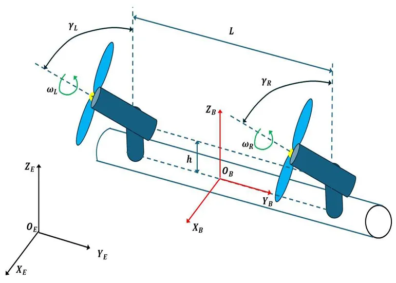
The diagram of the 6-DOF autonomous bicopter is given in . The inertial reference frame is denoted as $$O_{E} X_{E} Y_{E} Z_{E}$$. The body-fixed reference frame is denoted as $$O_{B} X_{B} Y_{B} Z_{B}$$. The rotation (Euler) angles around the axes of the inertial reference frame are denoted as $$\phi$$ (roll angle), $$\theta$$ (pitch angle) and $$\psi$$ (yaw angle).
The transformation matrix connecting the linear velocities of the bicopter in the inertial reference frame with the ones in the body-fixed reference frame is given by [
30]
The linear velocities vector of the bicopter in the inertial frame $$v_{E}$$ is connected to the velocities vector in the body-fixed frame through the relation
. Diagram of the 6-DOF autonomous bicopter.
It holds that $$v_{E} = R v_{B}$$, where $$v_{E} = \left[ \overset{\cdot}{x} , \overset{\cdot}{y} , \overset{\cdot}{x} \right]^{T}$$ is the linear velocities vector of the UAV in the inertial reference frame and $$v_{B} = \left[ u , v , w \right]^{T}$$ is the linear velocities vector of the UAV expressed in the body-fixed reference frame.
About the orientation (attitude) angles of the bicopter and the associated angular velocities it holds that
The angular velocities vector of the bicopter in the inertial frame $$\overset{\cdot}{\eta} = \left[ \overset{\cdot}{\phi} , \overset{\cdot}{\theta} , \overset{\cdot}{\phi} \right]^{T}$$ is connected to the angular velocities vector in the body-fixed frame $$\omega = \left[ p , q , r \right]^{T}$$ through the relation
The dynamic model of the bicopter comprises the following state vector: $$X = \left[ x_{E} , \overset{\cdot}{x}_{E} , \eta , \overset{\cdot}{\eta} \right]^{T}$$, where $$x_{E} = \left[ x , y , z \right]^{T}$$ are the cartesian coordinates of the center of gravity of the bicopter in the inertial reference frame, $$\overset{\cdot}{x}_{E} = \left[ \overset{\cdot}{x} , \overset{\cdot}{y} , \overset{\cdot}{z} \right]^{T}$$ are the linear velocities of the center of gravity of the bicopter in the inertial reference frame, $$\eta = \left[ \phi , \theta , \psi \right]^{T}$$ are the rotation angles of the bicopter around the axes of the inertial reference frame, and $$\overset{\cdot}{\eta} = \left[ \overset{\cdot}{\phi} , \overset{\cdot}{\theta} , \overset{\cdot}{\psi} \right]^{T}$$ are the angular velocities of the bicopter around the axes of the inertial reference frame [
4,
5,
6].
Thus, the state vector of the bicopter comprises state variables expressed exclusively in the inertial reference frame and is given by [
4]
The rotation speed of the right rotor is defined as $$\omega_{R}$$ and the tilting angle of this rotor is denoted as $$\gamma_{R}$$, The rotation speed of the left rotor is defined as $$\omega_{L}$$ and the tilting angle of this rotor is denoted as $$\gamma_{L}$$. The state equations which describe the dynamics of the bicopter are [
4]:
The control inputs vector of the bicopter is defined as $$u = \left[ u_{1} , u_{2} , u_{3} , u_{4} \right]^{T}$$ where
The parameters of the dynamic model of the bicopter are outlined in the following: $$m$$ is the mass of the bicopter, $$h$$ is the vertical distance between the center of gravity of the bicopter and the rotors’ plane, $$L$$ is the horizontal distance between the two rotors, $$K_{T}$$ is the thrust coefficient, $$I_{x x}$$ is the moment of inertia for rotation around the
x-axis of the inertial reference frame, $$I_{y y}$$ is the moment of inertia for rotation around the
y-axis of the inertial reference frame, $$I_{z z}$$ is the moment of inertia for rotation around the z-axis of the inertial reference frame, $$\omega_{R}$$ is the turn speed of the right rotor, $$\omega_{L}$$ is the turn speed of the left rotor, $$\gamma_{R}$$ is the tilting angle of the right rotor, $$\gamma_{L}$$ is the tilting angle of the left rotor.
Using the previously given definition about the state variables of the bicopter $$x_{i}$$, $$i=1,2,c\cdots,12$$ and the control inputs of this UAV $$u_{i}$$, $$i=1,\cdots,4,$$, the state-space description of the 6-DOF bicopter becomes:
Next, the control inputs of the bicopter are redefined as follows:
Through numerical operations one can confirm that the following relation holds
Thus, the state-space model of the bicopter is written in the following matrix form:
Concisely, the dynamic model of the bicopter can be written in the following nonlinear affine-in-the-input state-space form:
$$x{\in}R^{12\times1},f(x){\in}R^{12\times1},g(x){\in}R^{12\times6}\,\mathrm{and}\,v{\in}R^{6\times1}$$
3. Differential Flatness Properties of the 6-DOF Bicopter
The dynamic model of the bicopter of Equation (27) is differentially flat with flat outputs vector $$Y = \left[ x_{1} , x_{3} , x_{5} , x_{7} , x_{9} , x_{11} \right]^{T}$$ or $$Y = \left[ x , y , z , \phi , \theta , \psi \right]^{T}$$. A system is differentially flat if the following two conditions hold: (i) all its state variables and its control inputs can be written as differential functions of a selected subset its state vector elements which constitutes the flat outputs vector, (ii) the flat outputs and their time-derivatives are “differentially independent" which means that they are not connected through a relation in the form of an homogeneous differential equation.
From the odd-numbered state equations of the system one has:
Thus one can infer that the even-numbered state variables of the bicopter are differential functions of the system’s flat outputs, or
Besides, from the even-numbered state equations one has:
which equivalently gives
Thus, one infers that the control input variables of the bicopter are differential functions of the flat outputs vector of the system or
The differential flatness property is an implicit proof of the bicopter’s controllability. It also signifies that the bicopter’s dynamics can be transformed to the input-output linearized form through successive differentiations of its flat outputs. Moreover, it allows for solving the setpoints defition problem. First, one defines setpoints in an unconstraint manner for those state variables which coincide with the flat outputs of the system. These are the odd-numbered state variables $$x_{i}$$, $$i = 1 , 3 , 5 , 7 , 9 , 11$$. For the rest of the state variables, that is for the even-numbered state vector elements, setpoints are chosen using the differential relations which connect them with the flat outputs.
4. Approximate Linearization of the Bicopter Dynamics
The dynamic model of the bicopter, being in the nonlinear state-space form $$\overset{\cdot}{x} = f \left( x , u \right)$$, undergoes approximate linearization through first-order Taylor series expansion and through the computation of the associated Jacobian matrices. The linearization takes place at each sampling instance around the temporary operating point $$\left( x^{∗} , v^{∗} \right)$$, where $$x^{∗}$$ is the present value of the system’s state vector and $$v^{∗}$$ is the last sampled value of the control inputs vector. The modelling error which is due to the truncation of higher-order terms from the Taylor series expansion is considered to be a perturbation which is asymptotically compensated by the robustness of the control algorithm.
Thus, the system is brought to the equivalent linearized form
where $$A$$, $$B$$ are the Jacobian matrices of the bicopter which are given by
The control inputs gain matrix is $$g \left( x \right) = \left[ g_{1} , g_{2} , g_{3} , g_{4} , g_{5} , g_{6} \right]^{T}$$ and the Jacobian matrices of vectors $$g_{i} \left( x \right)$$, $$i = 1 , 2 , 3 , 4 , 6$$ are equal to the zero matrix $$0_{12 \times 12}$$. It is only Jacobian matrix $$\nabla_{x} g_{5} \left( x \right)$$ that has non-zero elements. The cumulative disturbance term $$\overset{\sim}{d}$$ may comprise: (i) the modelling error due to the truncation of higher-order terms from the Taylor series, (ii) model uncertainty and external perturbations, (iii) sensor measurement noise of any distribution.
The Jacobian matrices $$\nabla_{x} f \left( x \right) \mid_{\left( x^{∗} , v^{∗} \right)}$$ and $$\nabla_{x} g_{5} \left( x \right) \mid_{\left( x^{∗} , v^{∗} \right)}$$ are computed as follows:
5. Design of an H-Infinity Nonlinear Feedback Controller
5.1. Equivalent Linearized Kinematic-Dynamic Model of the Bicopter
After linearization around its current operating point, the dynamic model of the 6-DOF bicopter is written as
Parameter $$d_{1}$$ stands for the linearization error in the bicopter’s model that was given previously in Equation (39). The reference setpoints for the state vector of the aforementioned dynamic model are denoted by $$\begin{aligned}\mathbf{x_d}=[x_1^d,\cdots,x_{12}^d]\end{aligned}$$. Tracking of this trajectory is achieved after applying the control input $$u^{∗}$$. At every time instant the control input $$u^{∗}$$ is assumed to differ from the control input $$u$$ appearing in Equation (39) by an amount equal to $$\Delta u$$, that is $$u^{∗} = u + \Delta u$$
The dynamics of the controlled system described in Equation (39) can be also written as
and by denoting $$d_{3} = - B u^{∗} + d_{1}$$ as an aggregate disturbance term one obtains
By subtracting Equation (40) from Equation (42) one has
By denoting the tracking error as $$e = x - x_{d}$$ and the aggregate disturbance term as $$L \overset{\sim}{d} = d_{3} - d_{2}$$, the tracking error dynamics becomes
where $$L$$ is a disturbance inputs gain matrix. The above linearized form of the bicopter’s model can be efficiently controlled after applying an H-infinity feedback control scheme.
5.2. The Nonlinear H-Infinity Control
The initial nonlinear model of the bicopter is in the form
Linearization of the model of the bicopter is performed at each iteration of the control algorithm around its present operating point $$\left( x^{∗} , u^{∗} \right) = \left( x \left( t \right) , u \left( t - T_{s} \right) \right)$$. The linearized equivalent of the system is described by
where matrices $$A$$ and $$B$$ are obtained from the computation of the previously defined Jacobians and vector $$\overset{\sim}{d}$$ denotes disturbance terms due to linearization errors, while $$L$$ is a disturbance inputs gain matrix. The problem of disturbance rejection for the linearized model that is described by
where $$x \in R^{n}$$, $$u \in R^{m}$$, $$\overset{\sim}{d} \in R^{q}$$ and $$y \in R^{p}$$, cannot be handled efficiently if the classical LQR control scheme is applied. This is because of the existence of the perturbation term $$\overset{\sim}{d}$$. The disturbance term $$\overset{\sim}{d}$$ apart from modeling (parametric) uncertainty and external perturbations can also represent noise terms of any distribution.
In the $$H_{\infty}$$ control approach, a feedback control scheme is designed for trajectory tracking by the system’s state vector and simultaneous disturbance rejection, considering that the disturbance affects the system in the worst possible manner. The disturbances’ effects are incorporated in the following quadratic cost function:
The significance of the negative sign in the cost function’s term that is associated with the perturbation variable $$\overset{\sim}{d} \left( t \right)$$ is that the disturbance tries to maximize the cost function $$J \left( t \right)$$ while the control signal $$u \left( t \right)$$ tries to minimize it. The physical meaning of the relation given above is that the control signal and the disturbances compete to each other within a min-max differential game. This problem of min-max optimization can be written as $$\begin{aligned}min_umax_{\tilde{d}}J(u,\tilde{d})\end{aligned}$$.
The objective of the optimization procedure is to compute a control signal $$u \left( t \right)$$ which can compensate for the worst possible disturbance, that is externally imposed to the bicopter. The solution to the min-max optimization problem is directly related to the value of parameter $$\rho$$, while there is an upper bound in the disturbances magnitude that can be annihilated by the control signal.
5.3. Computation of the Feedback Control Gains
For the linearized system given by Equation (47) the cost function of Equation (48) is defined, where coefficient $$r$$ determines the penalization of the control input and weight coefficient $$\rho$$ determines the reward of the disturbances’ effects. It is assumed that (i) The energy that is transferred from the disturbances signal $$\overset{\sim}{d} \left( t \right)$$ is bounded, that is $$\int_{0}^{\infty} \overset{\sim}{d}^{T} \left( t \right) \overset{\sim}{d} \left( t \right) d t < \infty$$, (ii) matrices $$\left[ A , B \right]$$ and $$\left[ A , L \right]$$ are stabilizable, (iii) matrix $$\left[ A , C \right]$$ is detectable. In the case of a tracking problem the optimal feedback control law is given by
with $$e = x - x_{d}$$ to be the tracking error, and $$K=\frac{1}{r}B^{T}P$$ where
P is a positive definite symmetric matrix. As it will be proven in Section 6, matrix $$P$$ is obtained from the solution of the Riccati equation
where $$Q$$ is a positive semi-definite symmetric matrix. The worst case disturbance is given by
The solution of the H-infinity feedback control problem for the dynamic model of the bicopter and the computation of the worst case disturbance that the related controller can sustain, comes from superposition of Bellman’s optimality principle when considering that the bicopter is affected by two separate inputs (i) the control input $$u$$ (ii) the cumulative disturbance input $$\overset{\sim}{d} \left( t \right)$$. Solving the optimal control problem for $$u$$, that is for the minimum variation (optimal) control input that achieves elimination of the state vector’s tracking error, gives $$u=-\frac{1}{r}B^TPe$$. Equivalently, solving the optimal control problem for $$\overset{\sim}{d}$$, that is for the worst case disturbance that the control loop can sustain gives $$\tilde{d}=\frac{1}{\rho^{2}}{L^{T}}Pe$$.
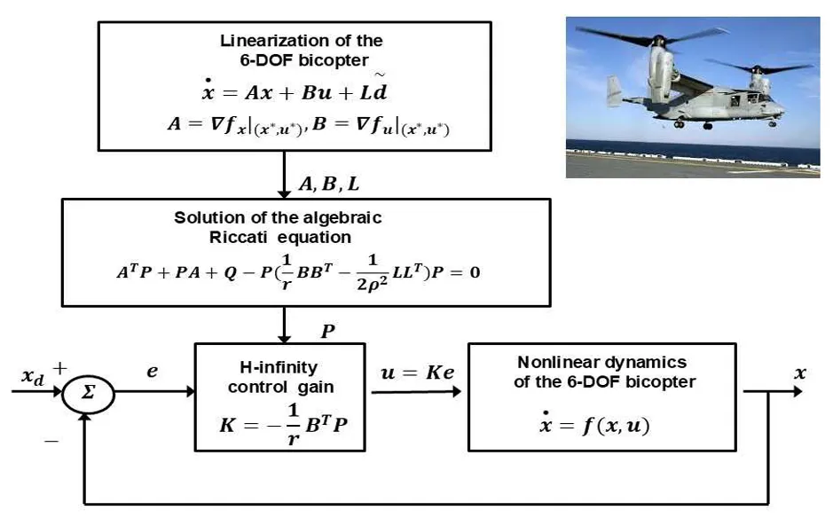
The diagram of the considered control loop for the 6-DOF bicopter is depicted in .
. Nonlinear optimal (H-infinity) control scheme and implementation stages for the bicopter.
6. Lyapunov Stability Analysis
Through Lyapunov stability analysis it will be shown that the proposed nonlinear control scheme assures $$H_{\infty}$$ tracking performance for the 6-DOF bicopter, and that in case of bounded disturbance terms asymptotic convergence to the reference setpoints is achieved. The tracking error dynamics for the bicopter is written in the form of Equation (44) $$\dot{e}=Ae+Bu+L\tilde{d}$$ where in the bicopter's case $$L=\in R^{12\times12}$$ is the disturbance inputs gain matrix. Variable $$\tilde{d}$$ denotes model uncertainties and external disturbances of the bicopter's dynamic model. The following Lyapunov function is considered
where $$e = x - x_{d}$$ is the tracking error. By differentiating with respect to time one obtains
The previous equation is rewritten as
Assumption 1. For given positive definite matrix $$Q$$ and coefficients $$r$$ and $$\rho$$ there exists a positive definite matrix $$P$$, which is the solution of the following matrix equation
Moreover, the following feedback control law is applied to the system
By substituting Equation (57) and Equation (58) one obtains
which after intermediate operations gives
or, equivalently
Lemma 1. The following inequality holds
Proof. The binomial $$(\rho\alpha-\frac{1}{\rho}b)^2$$ is considered. Expanding the left part of the above inequality one gets
The following substitutions are carried out: $$a = \overset{\sim}{d}$$ and $$b = e^{T} P L$$ and the previous relation becomes
Equation (65) is substituted in Equation (62) and the inequality is enforced, thus giving
Equation (66) shows that the $$H_{\infty}$$ tracking performance criterion is satisfied. The integration of $$\overset{\cdot}{V}$$ from $$0$$ to $$T$$ gives
Moreover, if there exists a positive constant $$M_{d} > 0$$ such that
then one gets
Thus, the integral $$\int_{0}^{\infty}\lvert\lvert e\rvert\rvert_{Q}^{2}dt$$ is bounded. Moreover, $$V \left( T \right)$$ is bounded and from the definition of the Lyapunov function $$V$$ in Equation (52) it becomes clear that $$e \left( t \right)$$ will be also bounded since $$e(t)\in\Omega_{e}=\{e|e^{T}Pe{\leq}2V(0)+\rho^{2}M_{d}\}$$. According to the above and with the use of Barbalat’s Lemma one obtains $$\lim_{t \rightarrow \infty} e \left( t \right) = 0$$. □
Through the stages of the stability proof one arrives at Equation (66) which shows that the H-infinity tracking performance criterion holds. By selecting the attenuation coefficient $$\rho$$ to be sufficiently small and in particular to satisfy $$\rho^2<||e||_Q^2/||\tilde{d}||^2$$ one has that the first derivative of the Lyapunov function is upper bounded by 0. This condition holds at each sampling instance and consequently global stability for the control loop of the bicopter can be concluded.
7. Multi-Loop Flatness-Based Control for the Autonomous Bicopter
Multi-loop flatness-based control is also proposed as an alternative method for the stabilization and autonomous navigation problem of the 6-DOF bicopter. The state variables of the 6-DOF bicopter are redefined as follows:
Using the redefinition of the state viarable of the 6-DOF bicopter, the state equations of the system comes to the following form:
Next, the new control inputs $$v_{1}$$ to $$v_{6}$$ are defined:
Once again, through numerical operations one can confirm that the following relation holds
This results into the following state-space description in matrix form:
Next, the state-space model of Equation (78) is written in the form of two cascading subsystems. To this end the following subvectors and submatrices are defined:
Subsysten $$\Sigma_{1}$$ with state vector $$z_{1 , 6} = \left[ z_{1} , z_{2} , z_{3} , z_{4} , z_{5} , z_{6} \right]^{T}$$, drift vector $$f_{1 , 6} \left( z_{1 , 6} \right) = 0_{6 \times 1}$$, control inputs gain matrix $$g_{1 , 6} \left( z_{1 , 6} \right) = I_{6 \times 6}$$ and virtual control inputs vector $$v_{1} = z_{7 , 12} = \left[ z_{7} , z_{8} , z_{9} , z_{10} , z_{11} , z_{12} \right]^{T}$$.
Subsystem $$\Sigma_{2}$$ with state vector $$z_{7 , 12} = \left[ z_{7} , z_{8} , z_{9} , z_{10} , z_{11} , z_{12} \right]^{T}$$, drift vector $$f_{7 , 12} = 0_{6 \times 1}$$, real control inputs vector $$v = \left[ v_{1} , v_{2} , v_{3} , v_{4} , v_{5} , v_{6} \right]^{T}$$ and control inputs gain matrix
Thus, the bicopter’s dynamics is written in the form of the chained subsystem: $$\Sigma_{1}$$ and $$\Sigma_{2}$$:
The integrated system of Equations (80) and (81) is differentially flat with flat outputs vector $$z_{1 , 6}$$.
Indeed from Equation (80) one has that $$z_{7 , 12} = \overset{\cdot}{z}_{1 , 6}$$ which means that $$z_{7 , 12}$$ is a differential function of the flat outputs vector $$z_{1 , 6}$$.
From Equation (81) one solves for the control inputs $$v$$. This gives
which signifies that control input $$v$$ is a differential function of the flat output $$z_{1 , 6}$$. Therefore, the integrated system of Equations (80) and (81) is differentially flat.
Differential flatness can be also proven for each one of the subsystems of Equations (80) and (81) is these are examined independently. For the subsystem of Equation (80) the flat output is taken to be $$y_{1} = z_{1 , 6}$$ and the virtual control inputs vector is defined to be $$v_{1} = z_{7 , 12}$$. Thus, solving Equation (80) for $$v_{1}$$ gives
which signifies that $$v_{1}$$ is a differential function of the flat outputs vector $$z_{1 , 6}$$. Consequently, the subsystem of Equation (80) is differentially flat.
For the subsystem of Equation (81) the flat output is taken to be $$y_{2} = z_{7 , 12}$$, while $$z_{1 , 6}$$ is considered to be a coefficients vector and the real control inputs vector is $$v$$. Thus, solving Equation (81) for $$v$$ gives
which signifies that $$v$$ is a differential function of the flat outputs vector $$z_{7 , 12}$$. Consequently, the subsystem of Equation (81) is also differentially flat.
The proof of differential flatness properties for the subsystems of Equations (80) and (81) means that: (i) these subsystems can be written in the input-output linearized form and (ii) a stabilizing feedback controller can be designed for each one of them by inverting their dynamics, as it is commonly done for input-output linearized flat systems.
8. Design of a Multi-Loop Flatness-Based Controller for the 6-DOF Bicopter
The bicopter’s dynamic model has been written in the form of the chained subsystems of Equations (80) and (81). For the subsystem of Equation (80) the stabilizing feedback control is taken to be
where $$z_{1 , 6}^{d}$$ is the setpoint for state vector $$z_{1 , 6}$$ and $$K_{1} \in R^{6 \times 6}$$ is a diagonal matrix with positive diagonal elements $$k_{i i , 1} > 0$$ for $$i=1,\cdots,6$$.
For the subsystem of Equation (81) the stabilizing feedback control is taken to be
where $$z_{7 , 12}^{d}$$ is the setpoint for state vector $$z_{7 , 12}$$ and $$K_{2} \in R^{6 \times 6}$$ is a diagonal matrix with positive diagonal elements $$k_{i i , 2} > 0$$ for $$i=1,\cdots,6.$$.
By substituting the feedback control input of Equation (85) into subsystem $$\Sigma_{1}$$ of Equation (80) and by defining the tracking error vector $$e_{1 , 6} = z_{1 , 6} - z_{1 , 6}^{d}$$ one gets asymptotically
By substituting the feedback control input of Equation (86) into subsystem $$\Sigma_{1}$$ of Equation (81) and by defining the tracking error vector $$e_{7 , 12} = z_{7 , 12} - z_{7 , 12}^{d}$$ one gets asymptotically
Consequently, the closed-loop system dynamics of the bicopter becomes asymptotically:
which comes to confirm that the bicopter state vector’s tracking error converges asymptotically to zero, and the system is globally asympotitcally stable.
Global asymptotic stability for the bicopter’s control loop can be also proven through Lyapunov stability analysis. To this end, the following Lyapunov function is defined:
By differentiating in time one gets:
Next, using the tracking error dynamics which was shown in Equation (89) one gets
or equivalently
with $$K_{1} > 0$$ and $$K_{2} > 0$$. Thus, one obtains
Consequently, the Lyapunov function of the bicopter’s control loop is strictly diminishing until it converges to 0 and thus the system is globally asymptotically stable.
9. Simulation Tests
9.1. Results from Nonlinear Optimal Control
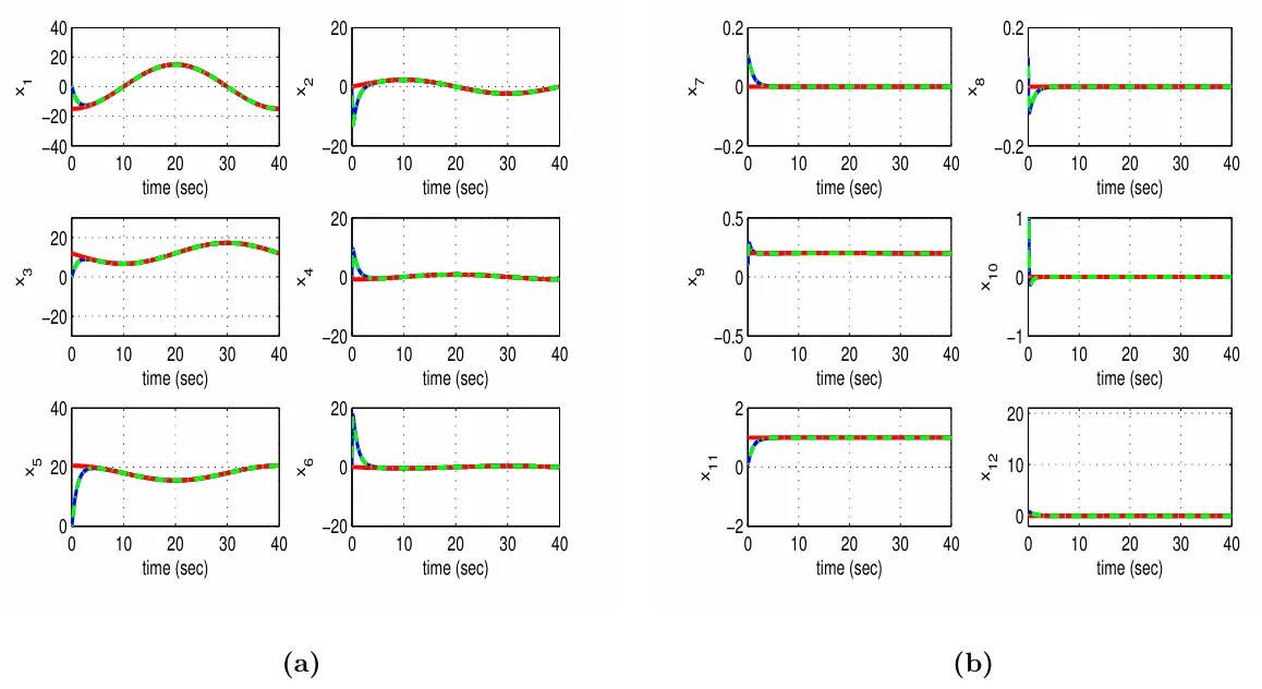
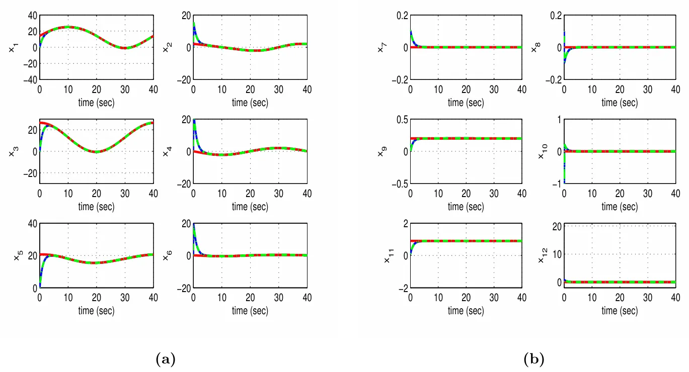
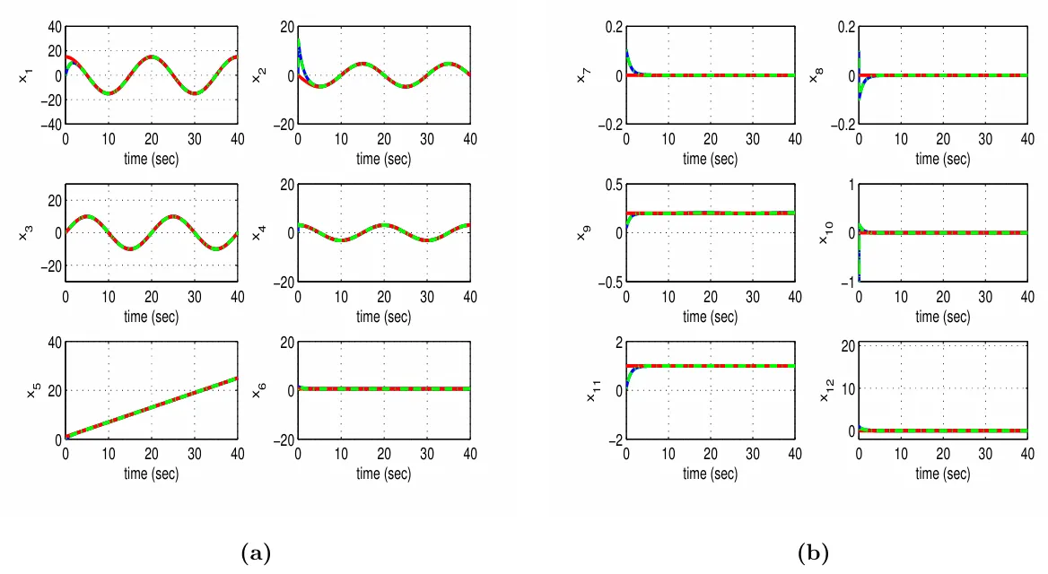
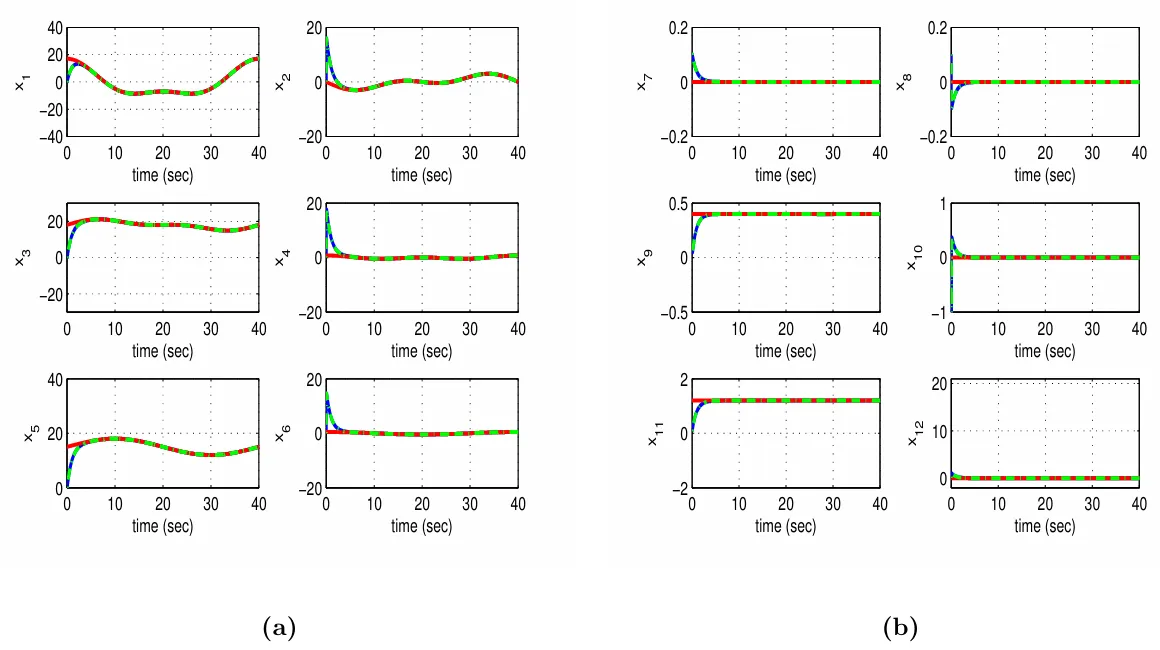
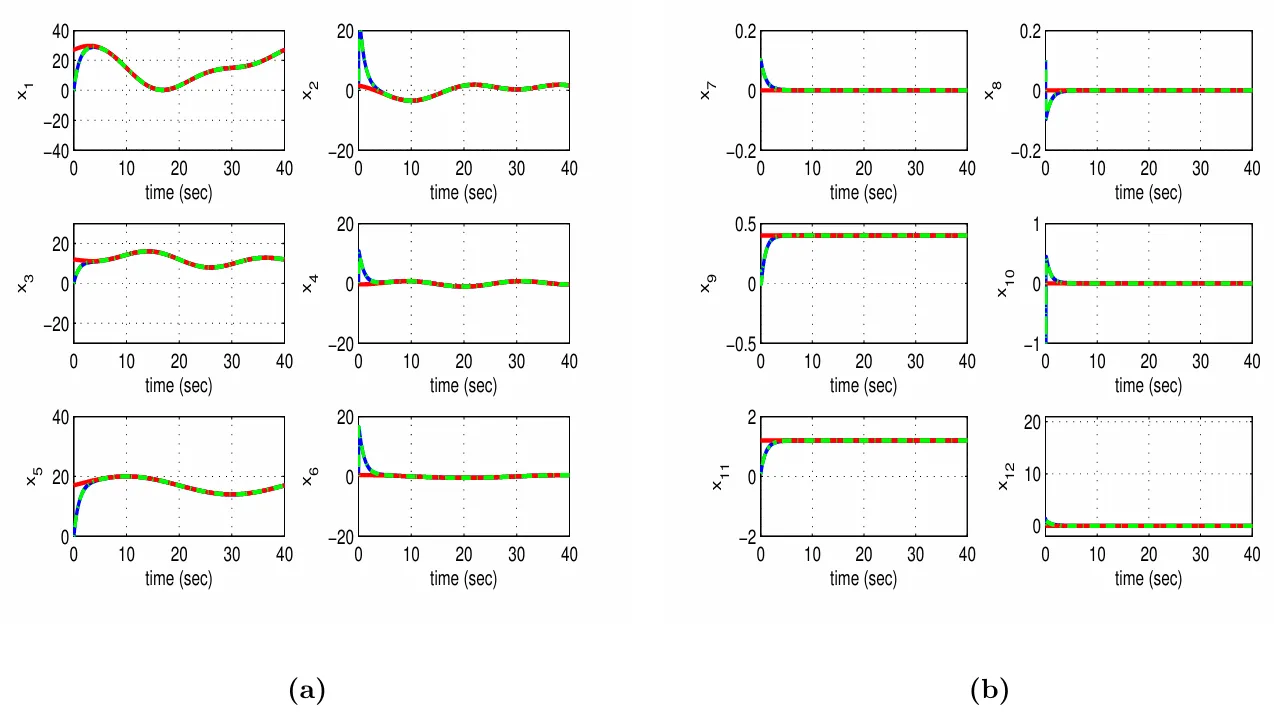
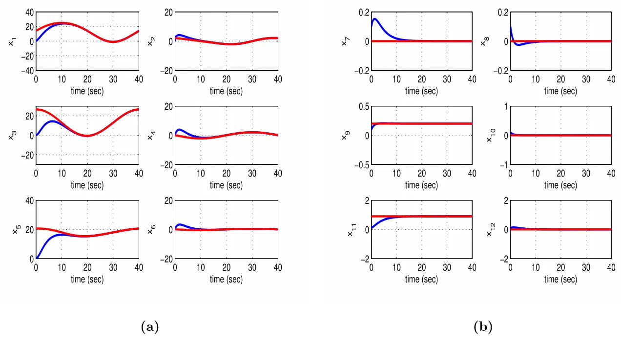
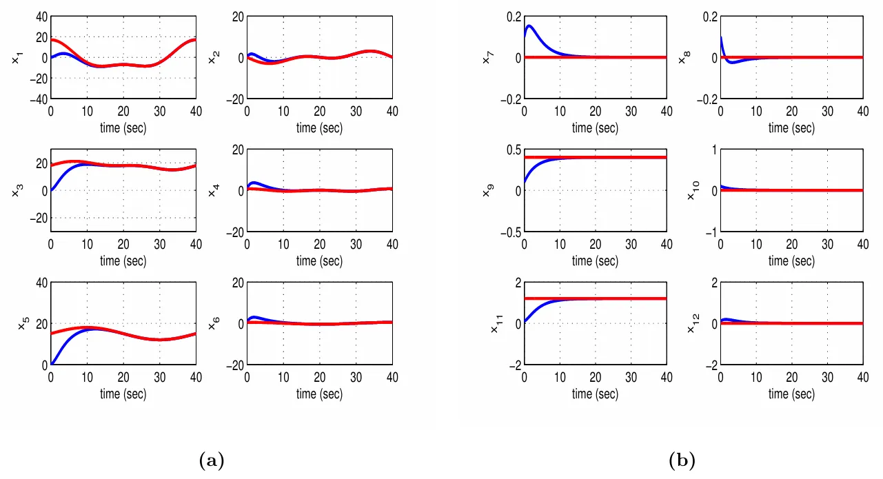
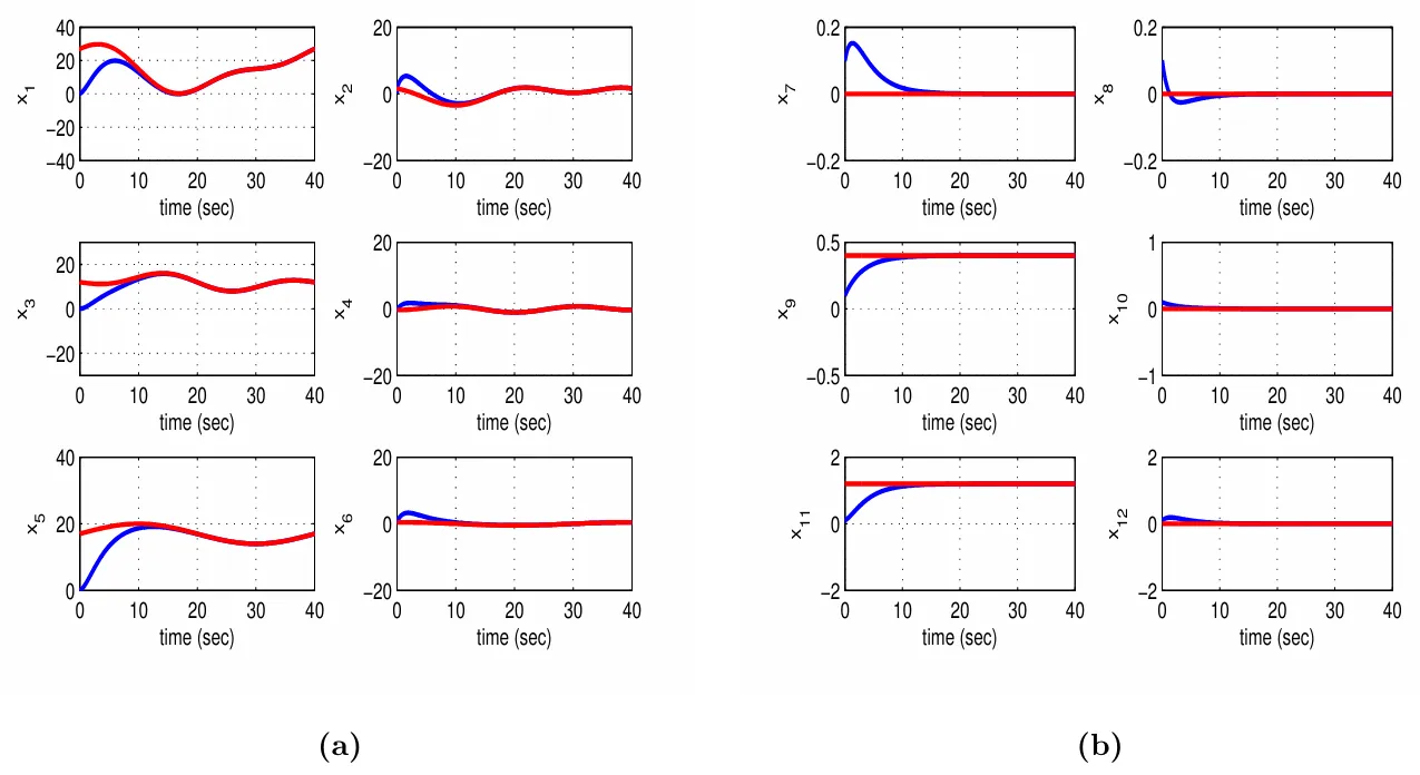
To confirm the fine performance of the proposed nonlinear optimal control method for the 6-DOF bicopter simulation experiments have been also performed. To apply this control scheme, the algebraic Riccati equation of Equation (57) had to be repetitively solved at each time-step of the control algorithm. The obtained results are depicted in , , , , , , , , , , , , , , and . State estimation is performed with the H-infinity Kalman Filter using as measurable outputs the odd numbered state variables $$x_{i}$$, $$i = 1 , 3 , 5 , 7 , 9 , 11$$. Indicative parametrization for the dynamic model of the bicopter can be found in [
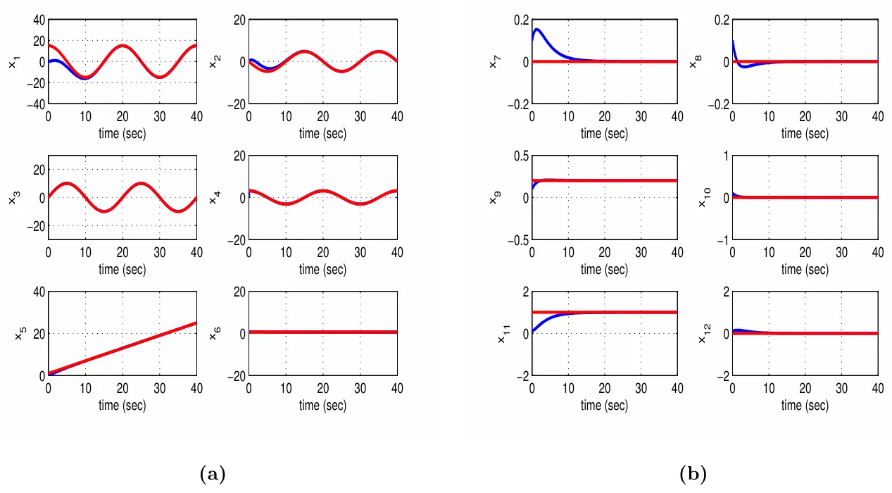
4] The values for the parameters of the dynamic model of the bicopter which have been used in the simulation experiments have been: $$m = 2$$ kg, $$K_{t} = 1 . 0$$, $$L = 1 . 0$$ m, $$I_{x x} = 1 . 0\, \mathrm{k g} \cdot \mathrm{m}^{2}$$, $$I_{y y} = 0 . 2\, \mathrm{k g} \cdot \mathrm{m}^{2}$$, $$I_{z z} = 0 . 2\, \mathrm{k g} \cdot \mathrm{m}^{2}$$ and $$g = 9 . 81\, \mathrm{m / s}^{2}$$. The real values of the state vector elements of the 6-DOF bicopter are printed in blue, the associated setpoints are marked in red while state estimates which have been provided by the H-infinity Kalman Filter are plotted in green. It can be noticed that the nonlinear optimal control method achieves fast and accurate tracking of setpoints by the state variables of the 6-DOF bicopter while keeping also moderate the variations of the control inputs. The transient performance of the control method is determined by the values of the coefficients $$r$$, $$\rho$$ and $$Q$$ of the above-noted Riccati equation. For relatively small values of gain $$r$$ the tracking error of the state variables is eliminated, while for relatively large values of the diagonal elements of matrix $$Q$$ fast convergence of the state variables to setpoints is enabled. Moreover, the smallest value of the attenuation coefficient $$\rho$$ for which one obtains a valid solution from the method’s Riccati equation (in the form of a positive definite and symmetric matrix $$P$$) is the one that gives to the control loop its maximum robustness.
Compared to other nonlinear control schemes that one could have considered for treating the control problem of the 6-DOF bicopter it can be stated that the article’s nonlinear optimal control scheme exhibits specific advantages. Unlike global linearization-based control methods (Lie algebra-based control and flatness-based control with transformation into canonical forms) the new nonlinear optimal control method avoids changes of state variables and complicated state-space model transformations. Besides, it does not need inverse transformations for computing the control inputs that should be applied to the initial nonlinear state-space model of the system and in this manner singularity issues are also avoided. Unlike Nonlinear Model Predictive Control, the proposed nonlinear optimal control method is of proven global stability and the convergence of its iterative search for the optimum does not depend on initial conditions and on ad-hoc parametrization of the controller. Unlike sliding-mode control and backstepping control, in the new nonlinear optimal control method there is no need the controlled system to be found or to be transformed into a specific state-space form. For instance, in sliding-mode control the selection of sliding surfaces becomes an intuitive procedure if the system is not previously transformed into the input-output linearized form. Furthermore, the application of backstepping control is hindered if the controlled system is not found in the backstepping integral (strict feedback) form. Compared to PID control approaches the new nonlinear optimal control method is of proven global stability, performs well at changes of operating points and does not use empirical knowledge and ad-hoc procedures for selecting the feedback gains of the controller. Finally, compared to multi-model feedback control the new nonlinear optimal control method is computationally more efficient because it does not need to linearize around multiple operating points and because it does not have to solve multiple Riccati equations or LMIs so as to compute the feedback control signals.
Figure 3. Tracking of setpoint 1 by the 6-DOF bicopter with the use of nonlinear optimal control: (<b>a</b>) convergence of state variables x<sub>1</sub> to x<sub>6</sub> (blue lines) to the associated setpoints (red lines) and estimated values provided by Kalman Filtering (green lines) (<b>b</b>) convergence of state variables x<sub>7</sub> to x<sub>12</sub> (blue lines) to the associated setpoints (red lines) and estimated values provided by Kalman Filtering (green lines).
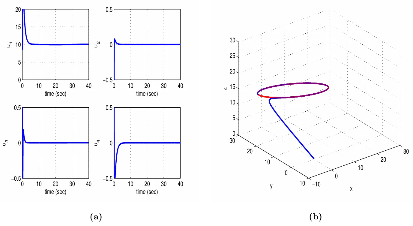
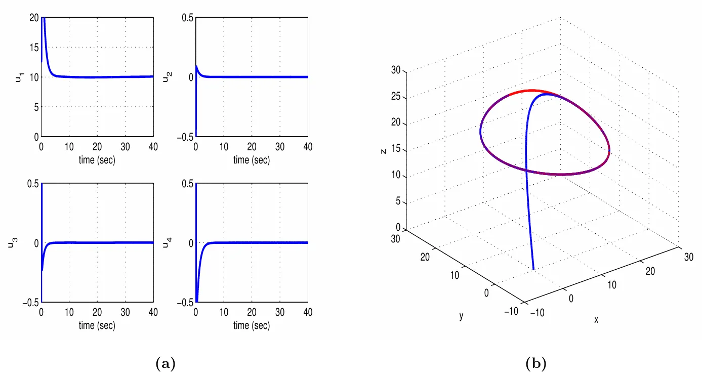
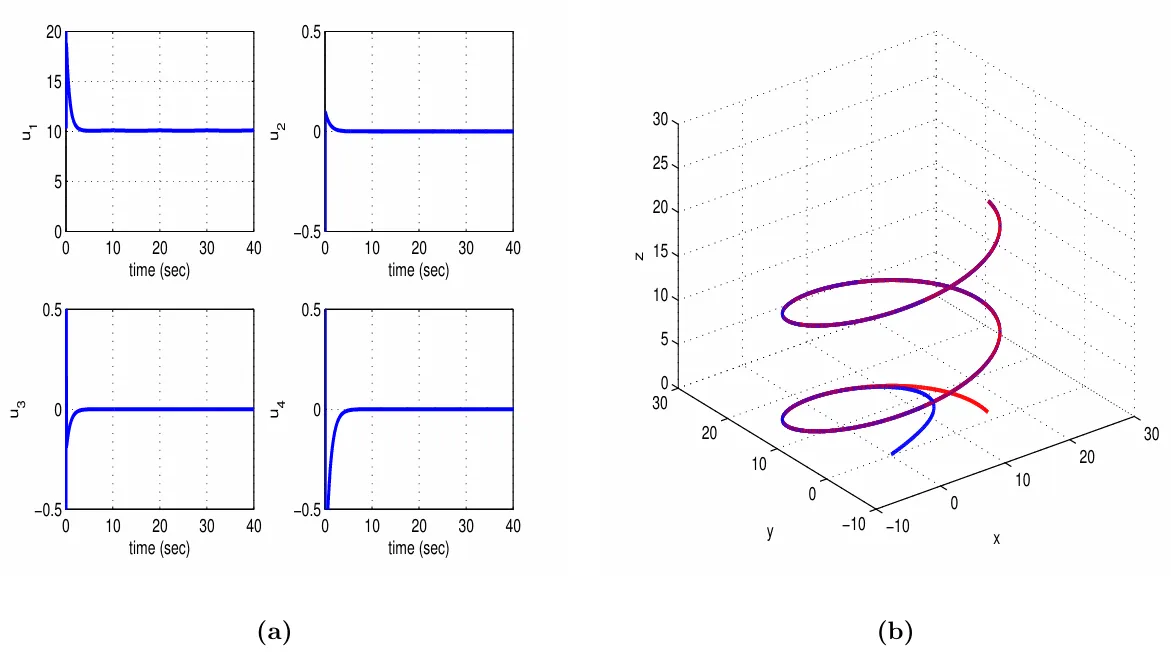
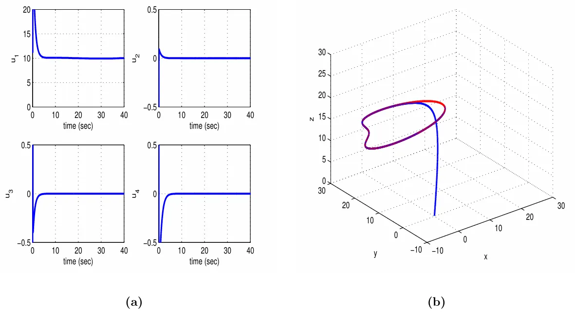
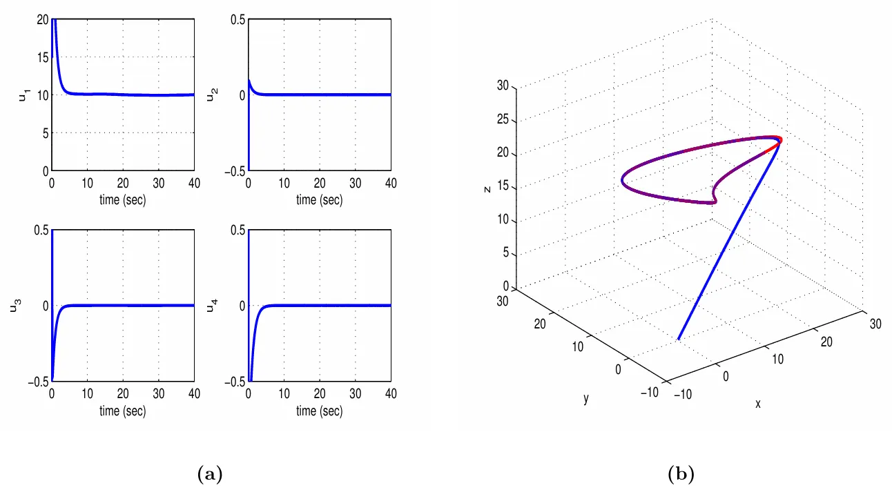
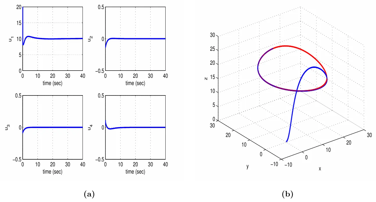
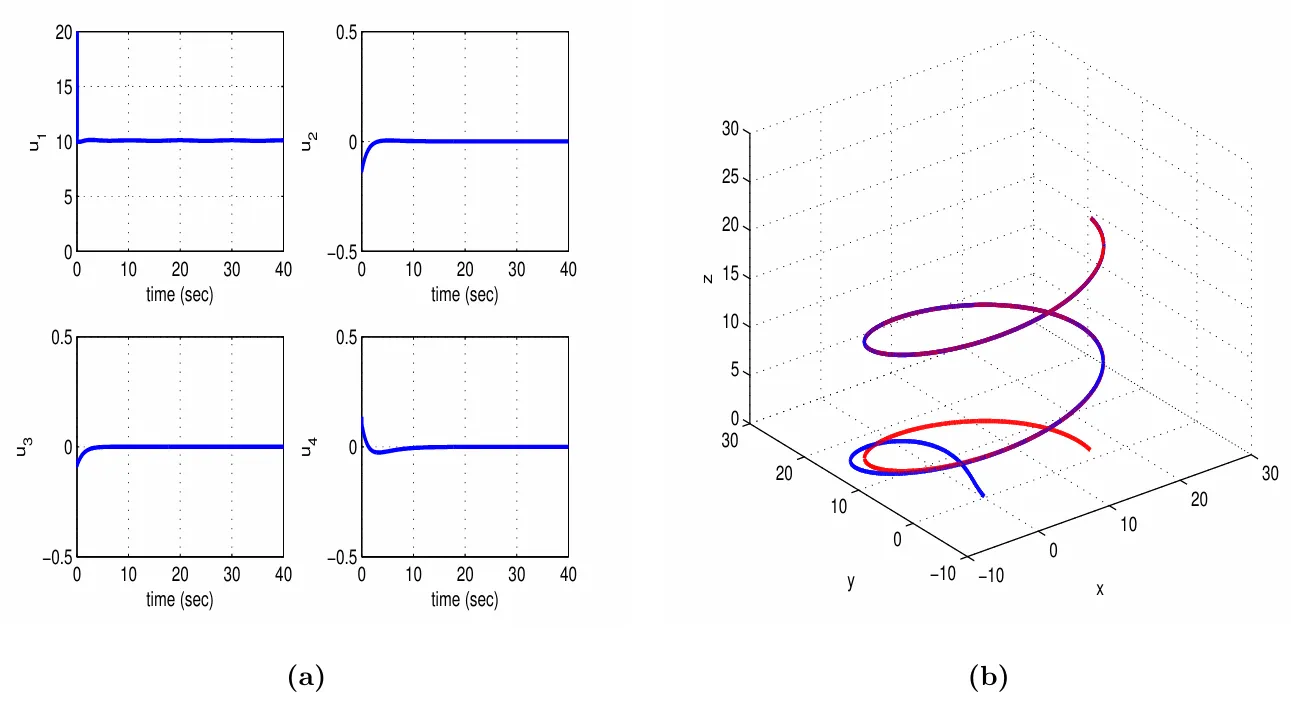
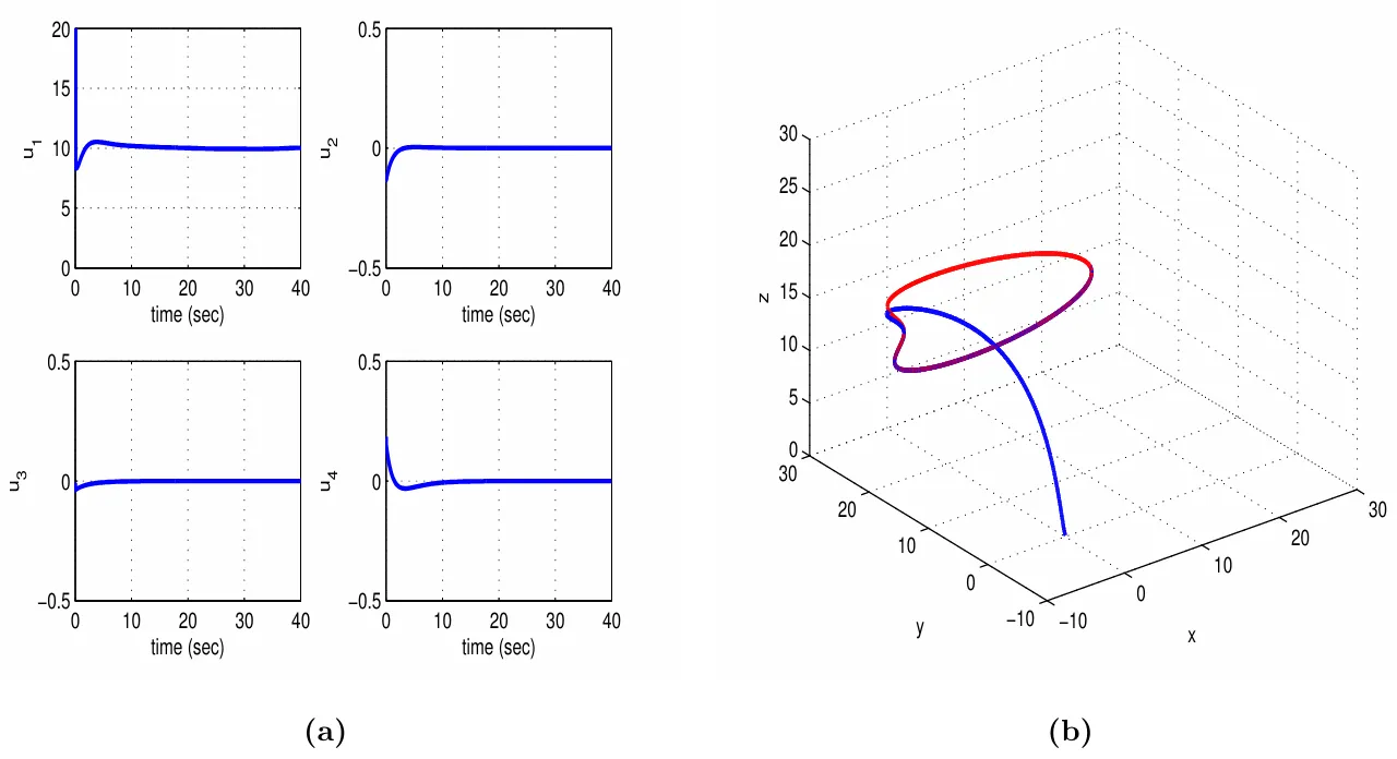
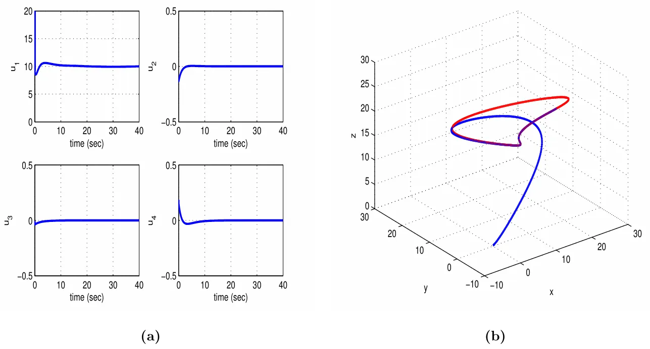
Figure 4. Tracking of setpoint 1 by the 6-DOF bicopter with the use of nonlinear optimal control: (<b>a</b>) variations of the control inputs u<sub>1</sub> and u<sub>4</sub> (blue lines) (<b>b</b>) convergence of the path of the bicopter’s center of gravity (blue line) to its reference trajectory in the XYZ cartesian space (red line).
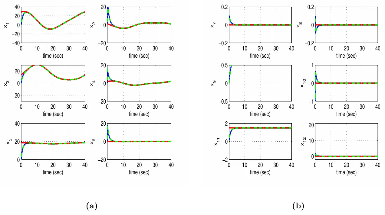
Figure 5. Tracking of setpoint 2 by the 6-DOF bicopter with the use of nonlinear optimal control: (<b>a</b>) convergence of state variables x<sub>1</sub> to x<sub>6</sub> (blue lines) to the associated setpoints (red lines) and estimated values provided by Kalman Filtering (green lines) (<b>b</b>) convergence of state variables x<sub>7</sub> to x<sub>12</sub> (blue lines) to the associated setpoints (red lines) and estimated values provided by Kalman Filtering (green lines).
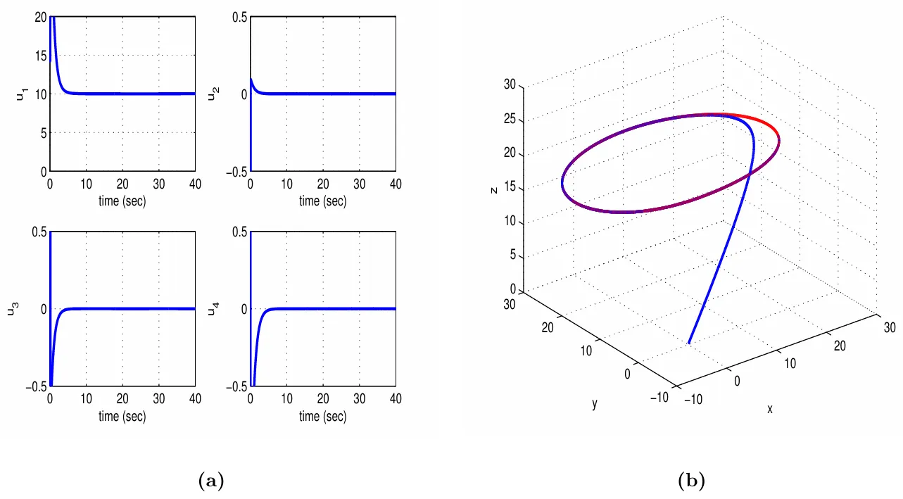
Figure 6. Tracking of setpoint 2 by the 6-DOF bicopter with the use of nonlinear optimal control: (<b>a</b>) variations of the control inputs u<sub>1</sub> and u<sub>4</sub> (blue lines) (<b>b</b>) convergence of the path of the bicopter’s center of gravity (blue line) to its reference trajectory in the XYZ cartesian space (red line).
Figure 7. Tracking of setpoint 3 by the 6-DOF bicopter with the use of nonlinear optimal control: (<b>a</b>) convergence of state variables x<sub>1</sub> to x<sub>6</sub> (blue lines) to the associated setpoints (red lines) and estimated values provided by Kalman Filtering (green lines) (<b>b</b>) convergence of state variables x<sub>7</sub> to x<sub>12</sub> (blue lines) to the associated setpoints (red lines) and estimated values provided by Kalman Filtering (green lines).
Figure 8. Tracking of setpoint 3 by the 6-DOF bicopter with the use of nonlinear optimal control: (<b>a</b>) variations of the control inputs u<sub>1</sub> and u<sub>4</sub> (blue lines) (<b>b</b>) convergence of the path of the bicopter’s center of gravity (blue line) to its reference trajectory in the XYZ cartesian space (red line).
Figure 9. Tracking of setpoint 4 by the 6-DOF bicopter with the use of nonlinear optimal control: (<b>a</b>) convergence of state variables x<sub>1</sub> to x<sub>6</sub> (blue lines) to the associated setpoints (red lines) and estimated values provided by Kalman Filtering (green lines) (<b>b</b>) convergence of state variables x<sub>7</sub> to x<sub>12</sub> (blue lines) to the associated setpoints (red lines) and estimated values provided by Kalman Filtering (green lines).
Figure 10. Tracking of setpoint 4 by the 6-DOF bicopter with the use of nonlinear optimal control: (<b>a</b>) variations of the control inputs u<sub>1</sub> and u<sub>4</sub> (blue lines) (<b>b</b>) convergence of the path of the bicopter’s center of gravity (blue line) to its reference trajectory in the XYZ cartesian space (red line).
Figure 11. Tracking of setpoint 5 by the 6-DOF bicopter with the use of nonlinear optimal control: (<b>a</b>) convergence of state variables x<sub>1</sub> to x<sub>6</sub> (blue lines) to the associated setpoints (red lines) and estimated values provided by Kalman Filtering (green lines) (<b>b</b>) convergence of state variables x<sub>7</sub> to x<sub>12</sub> (blue lines) to the associated setpoints (red lines) and estimated values provided by Kalman Filtering (green lines).
Figure 12. Tracking of setpoint 5 by the 6-DOF bicopter with the use of nonlinear optimal control: (<b>a</b>) variations of the control inputs u<sub>1</sub> and u<sub>4</sub> (blue lines) (<b>b</b>) convergence of the path of the bicopter’s center of gravity (blue line) to its reference trajectory in the XYZ cartesian space (red line).
Figure 13. Tracking of setpoint 6 by the 6-DOF bicopter with the use of nonlinear optimal control: (<b>a</b>) convergence of state variables x<sub>1</sub> to x<sub>6</sub> (blue lines) to the associated setpoints (red lines) and estimated values provided by Kalman Filtering (green lines) (<b>b</b>) convergence of state variables x<sub>7</sub> to x<sub>12</sub> (blue lines) to the associated setpoints (red lines) and estimated values provided by Kalman Filtering (green lines).
Figure 14. Tracking of setpoint 6 by the 6-DOF bicopter with the use of nonlinear optimal control: (<b>a</b>) variations of the control inputs u<sub>1</sub> and u<sub>4</sub> (blue lines) (<b>b</b>) convergence of the path of the bicopter’s center of gravity (blue line) to its reference trajectory in the XYZ cartesian space (red line).
Figure 15. Tracking of setpoint 7 by the 6-DOF bicopter with the use of nonlinear optimal control: (<b>a</b>) convergence of state variables x<sub>1</sub> to x<sub>6</sub> (blue lines) to the associated setpoints (red lines) and estimated values provided by Kalman Filtering (green lines) (<b>b</b>) convergence of state variables x<sub>7</sub> to x<sub>12</sub> (blue lines) to the associated setpoints (red lines) and estimated values provided by Kalman Filtering (green lines).
Figure 16. Tracking of setpoint 7 by the 6-DOF bicopter with the use of nonlinear optimal control: (<b>a</b>) variations of the control inputs u<sub>1</sub> and u<sub>4</sub> (blue lines) (<b>b</b>) convergence of the path of the bicopter’s center of gravity (blue line) to its reference trajectory in the XYZ cartesian space (red line).
Figure 17. Tracking of setpoint 8 by the 6-DOF bicopter with the use of nonlinear optimal control: (<b>a</b>) convergence of state variables x<sub>1</sub> to x<sub>6</sub> (blue lines) to the associated setpoints (red lines) and estimated values provided by Kalman Filtering (green lines) (<b>b</b>) convergence of state variables x<sub>7</sub> to x<sub>12</sub> (blue lines) to the associated setpoints (red lines) and estimated values provided by Kalman Filtering (green lines).
Figure 18. Tracking of setpoint 8 by the 6-DOF bicopter with the use of nonlinear optimal control: (<b>a</b>) variations of the control inputs u<sub>1</sub> and u<sub>4</sub> (blue lines) (<b>b</b>) convergence of the path of the bicopter’s center of gravity (blue line) to its reference trajectory in the XYZ cartesian space (red line).
To elaborate on the tracking performance and on the robustness of the proposed nonlinear optimal control method for 6-DOF bicopter the following Tables are given: (i)
Table 1 which provides information about the accuracy of tracking of the reference setpoints by the state variables of the 6-DOF bicopter’s state-space model, (ii)
Table 2 which provides information about the robustness of the control method to parametric changes in the model of the 6-DOF bicopter, for instance change in mass $$m$$, (iii)
Table 3 which provides the convergence times of the 6-DOF bicopter’s state variables to the associated setpoints.
Table 1.
Nonlinear optimal control. Tracking RMSE for the 6-DOF bicopter in the disturbance-free case.
|
RMSEx1 |
RMSEx2 |
RMSEx3 |
RMSEx7 |
RMSEx8 |
RMSEx9 |
| setpoint1 |
0.0008 |
0.0001 |
0.0002 |
0.0001 |
0.0001 |
0.0001 |
| setpoint2 |
0.0002 |
0.0001 |
0.0005 |
0.0001 |
0.0001 |
0.0001 |
| setpoint3 |
0.0009 |
0.0003 |
0.0007 |
0.0001 |
0.0001 |
0.0001 |
| setpoint4 |
0.0008 |
0.0002 |
0.0006 |
0.0001 |
0.0001 |
0.0001 |
| setpoint5 |
0.0006 |
0.0002 |
0.0002 |
0.0001 |
0.0001 |
0.0001 |
| setpoint6 |
0.0006 |
0.0002 |
0.0002 |
0.0001 |
0.0001 |
0.0001 |
| setpoint7 |
0.0002 |
0.0001 |
0.0003 |
0.0001 |
0.0001 |
0.0001 |
| setpoint8 |
0.0002 |
0.0001 |
0.0002 |
0.0001 |
0.0001 |
0.0001 |
Table 2.
Nonlinear optimal control.Tracking RMSE for the 6-DOF bicopter in the case of disturbances.
| ∆a% |
RMSEx1 |
RMSEx2 |
RMSEx3 |
RMSEx7 |
RMSEx8 |
RMSEx9 |
| 0% |
0.0002 |
0.0001 |
0.0005 |
0.0001 |
0.0001 |
0.0001 |
| 10% |
0.0003 |
0.0001 |
0.0005 |
0.0001 |
0.0001 |
0.0001 |
| 20% |
0.0004 |
0.0001 |
0.0005 |
0.0001 |
0.0001 |
0.0001 |
| 30% |
0.0005 |
0.0001 |
0.0006 |
0.0001 |
0.0001 |
0.0001 |
| 40% |
0.0005 |
0.0001 |
0.0006 |
0.0001 |
0.0001 |
0.0001 |
| 50% |
0.0006 |
0.0001 |
0.0006 |
0.0001 |
0.0001 |
0.0001 |
| 60% |
0.0006 |
0.0001 |
0.0007 |
0.0001 |
0.0001 |
0.0001 |
Table 3.
Nonlinear optimal control.Convergence time (s) for the 6-DOF bicopter.
|
Ts x1 |
Ts x2 |
Ts x3 |
Ts x7 |
Ts x8 |
Ts x9 |
| setpoint1 |
3.0 |
3.0 |
2.5 |
3.0 |
3.0 |
1.0 |
| setpoint2 |
2.5 |
3.0 |
3.0 |
2.5 |
3.0 |
2.5 |
| setpoint3 |
0.5 |
0.5 |
2.0 |
2.5 |
3.0 |
2.5 |
| setpoint4 |
2.5 |
3.5 |
0.5 |
2.5 |
3.0 |
2.5 |
| setpoint5 |
0.5 |
0.5 |
3.5 |
2.5 |
2.5 |
3.5 |
| setpoint6 |
2.5 |
3.5 |
3.5 |
2.5 |
3.0 |
3.0 |
| setpoint7 |
3.5 |
3.5 |
2.5 |
2.5 |
3.0 |
2.5 |
| setpoint8 |
3.5 |
3.0 |
2.5 |
2.5 |
3.0 |
2.5 |
9.2. Results from Multi-Loop Flatness-Based Control
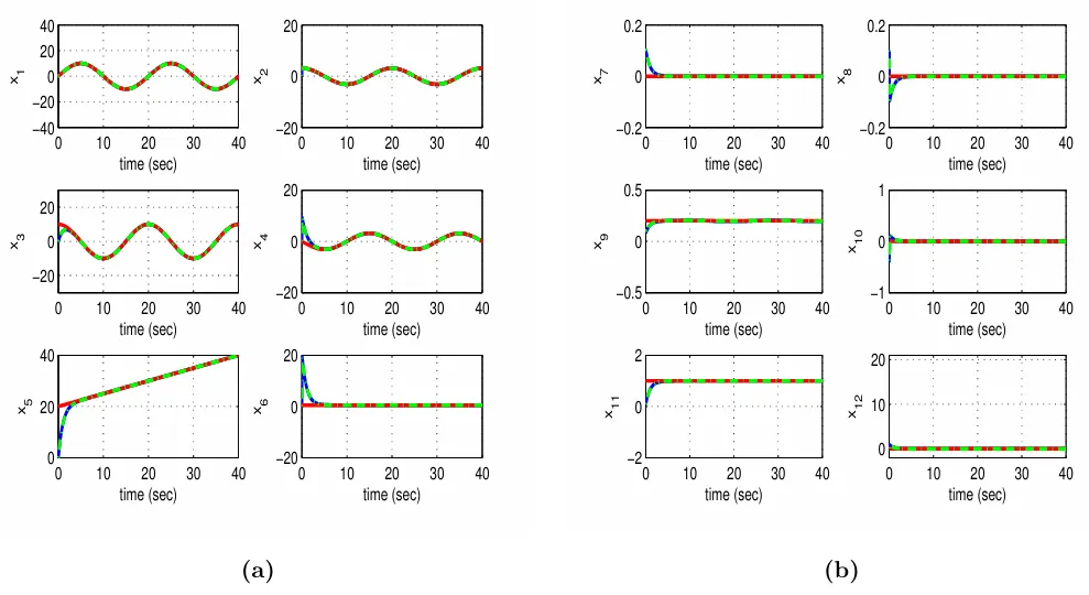
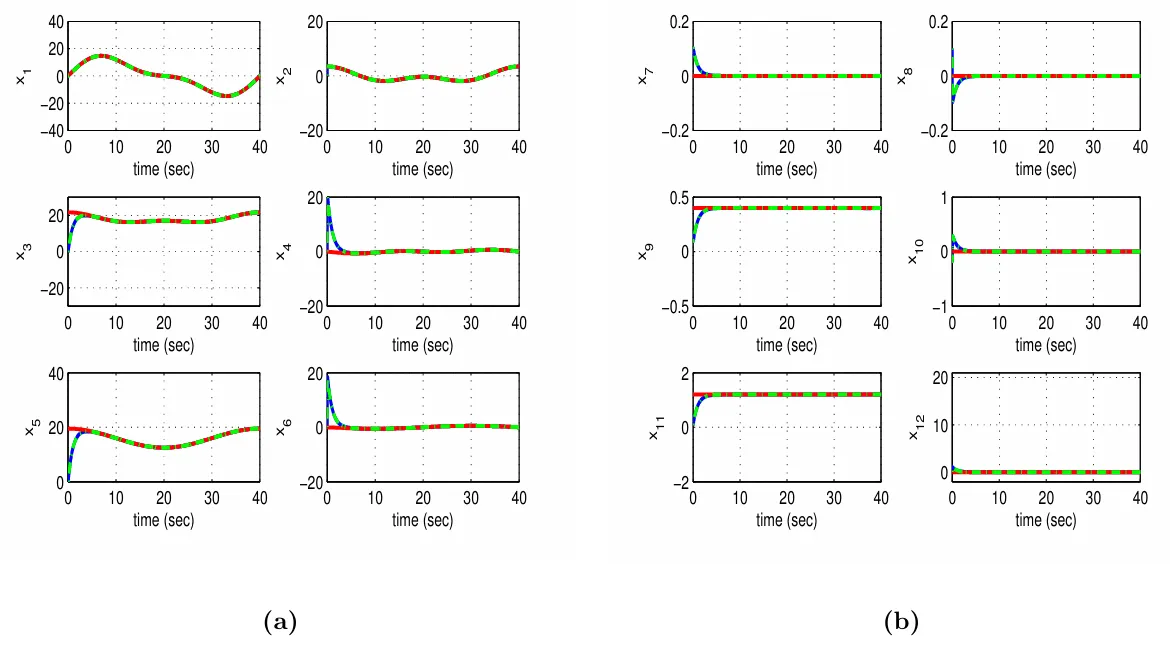
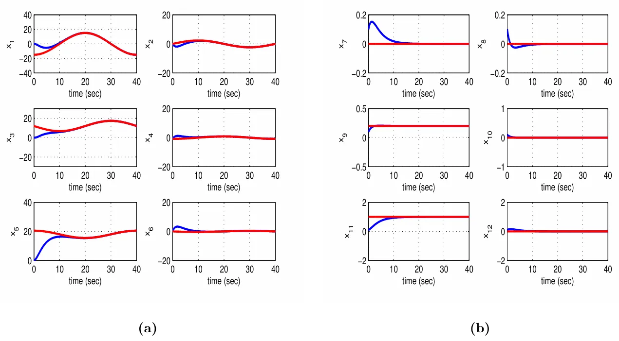
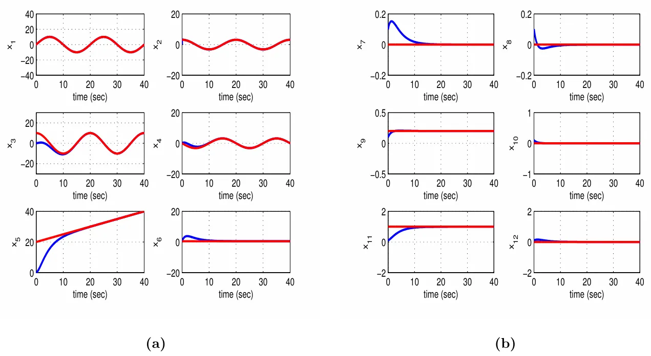
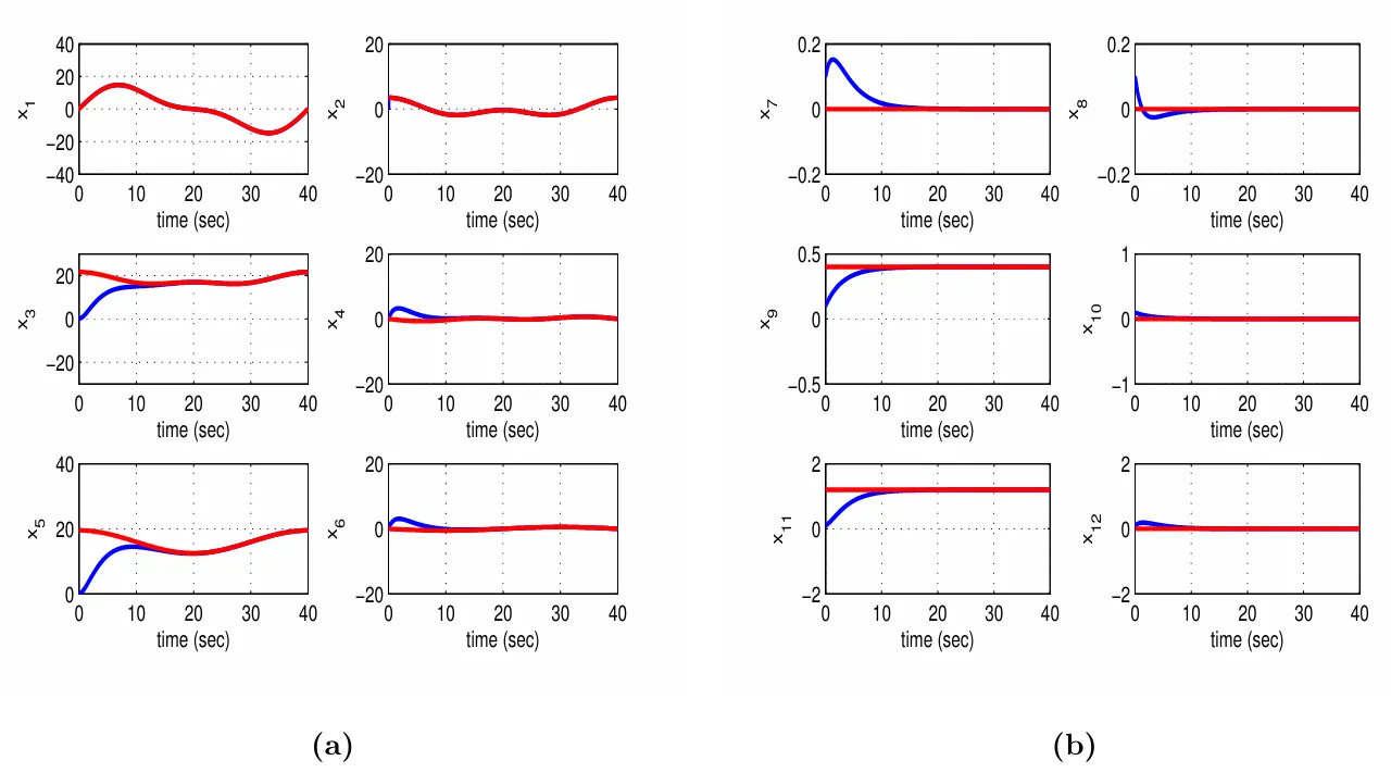
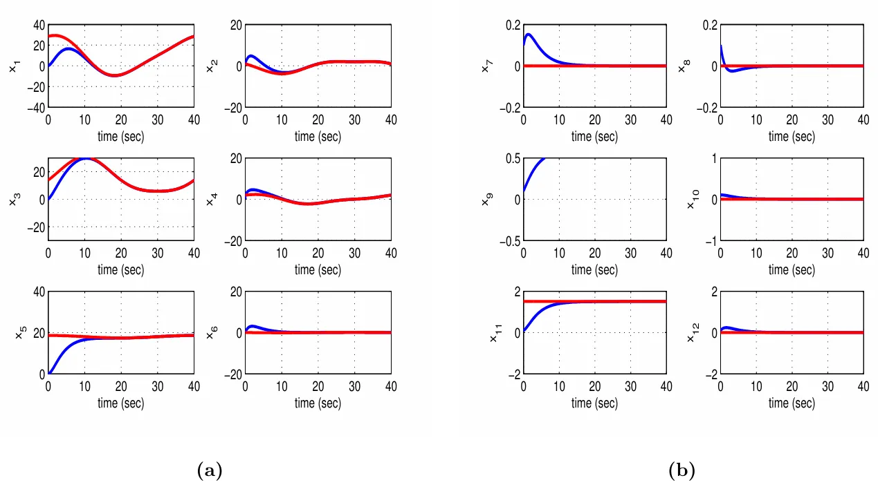
The fine performance of the multi-loop flatness-based control method has been further confirmed through simulation experiments. Under this control scheme the stabilization and autonomous navigation of the bicopter becomes a simple procedure. It suffices to assign positive values to the diagonal elments of the two diagonal feedback gain matrices $$K_{1}$$ and $$K_{2}$$ of the two chained subsystems in which the state-space model of the bicopter is decomposed. The obtained results are depicted in , , , , , , , , , , , , , , and . The multi-loop flatness-based control method allows for treating also the setpoints definition problem for the bicopter. Setpoints are chosen in an unconstrained manner for the state vector of the first subsystem. Next, the virtual control inputs vector of the first subsystem becomes setpoints vector for the second subsystem. The speed of convergence of the state variables of the two subsystems to their setpoints depends on the values of the diagonal elements of gain matrices $$K_{1}$$ and $$K_{2}$$. An advantage of the multi-loop flatness-based control method is that it avoids changes of state variables and complicated state-space model transformations.
The feedback control scheme, which is followed for the cascading subsystems that constitute the dynamic model of the 6-DOF bicopter and which is based on inversion of the subsystems’ dynamics of this aerial drone, is equally robust to sliding-mode control in which the switching control term has been substituted by a saturation function. One can easily confirm this for the first-order $$i$$-th subsystem of the form $$\overset{\cdot}{z}_{i} = f_{i} \left( z_{i} \right) + g_{i} \left( z_{i} \right) v_{i}$$ by defining the sliding surface $$s_{i} = e_{i} = z_{1} - z_{i}^{d}$$ and the associated sliding mode controller $$v_{i} = \hat{g}_{i} \left( z_{i} \right)^{- 1} \left[ \overset{\cdot}{z}_{i}^{d} - \hat{f}_{i} \left( z_{i} \right) - K_{i} s g n \left( z_{i} - z_{i}^{d} \right) \right]$$ which after substituting the $$s g n \left( s_{i} \right)$$ function with the saturation $$s a t \left( s_{i} \right)$$ function becomes $$v_{i} = \hat{g}_{i} \left( z_{i} \right)^{- 1} \left[ \overset{\cdot}{z}_{i}^{d} - \hat{f}_{i} \left( z_{i} \right) - K_{i} \left( z_{i} - z_{i}^{d} \right) \right]$$. The latter relation coincides with the flatness-based control in successive loops for the $$i$$-th subsystem under uncertainty (with use of the estimated functions $$\hat{f}_{i} \left( z_{i} \right)$$ and $$\hat{g}_{i} \left( z_{i} \right)$$) which is computed by the article’s control method. Therefore, the proposed flatness-based control method in successive loops provides sufficient robustness margins which enable the reliable and safe functioning of the 6-DOF bicopter under reasonable levels of model uncertainty or external perturbations.
Figure 19. Tracking of setpoint 1 by the 6-DOF bicopter with the use of multi-loop flatness-based control: (<b>a</b>) convergence of state variables x<sub>1</sub> to x<sub>6</sub> (blue lines) to the associated setpoints (red lines) and estimated values provided by Kalman Filtering (<b>b</b>) convergence of state variables x<sub>7</sub> to x<sub>12</sub> (blue lines) to the associated setpoints (red lines) and estimated values provided by Kalman Filtering.
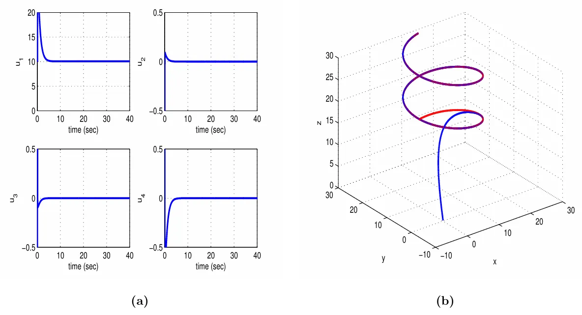
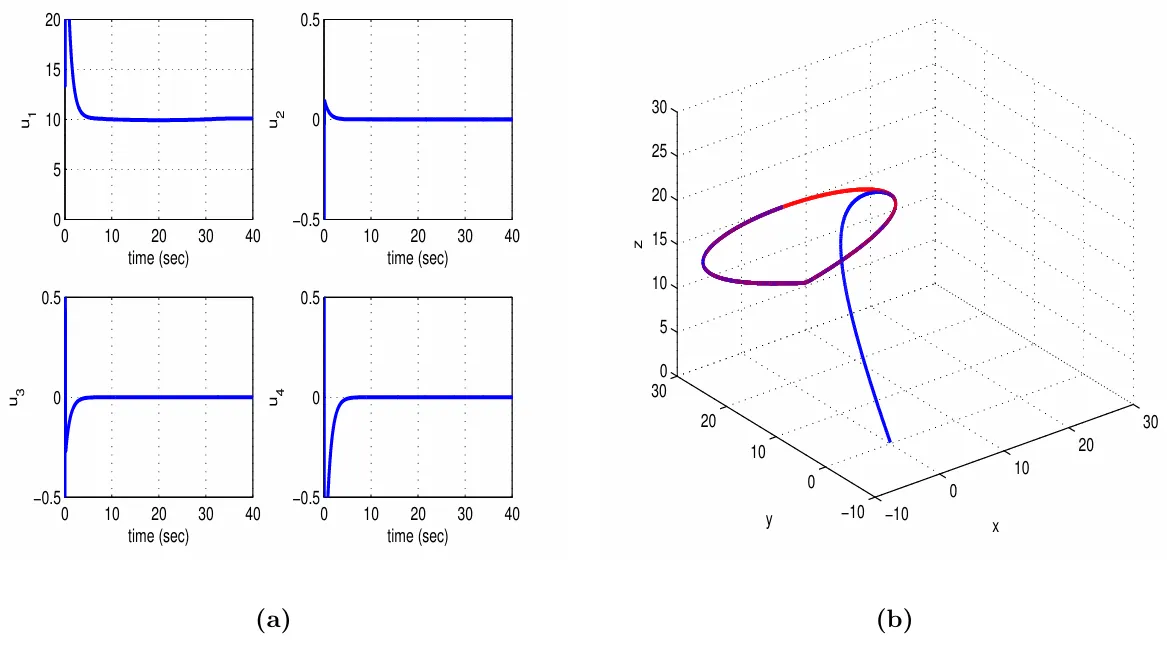
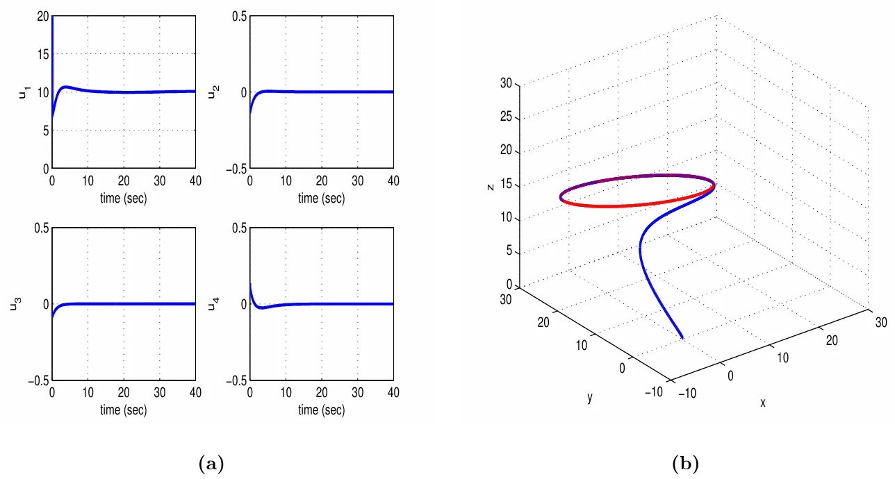
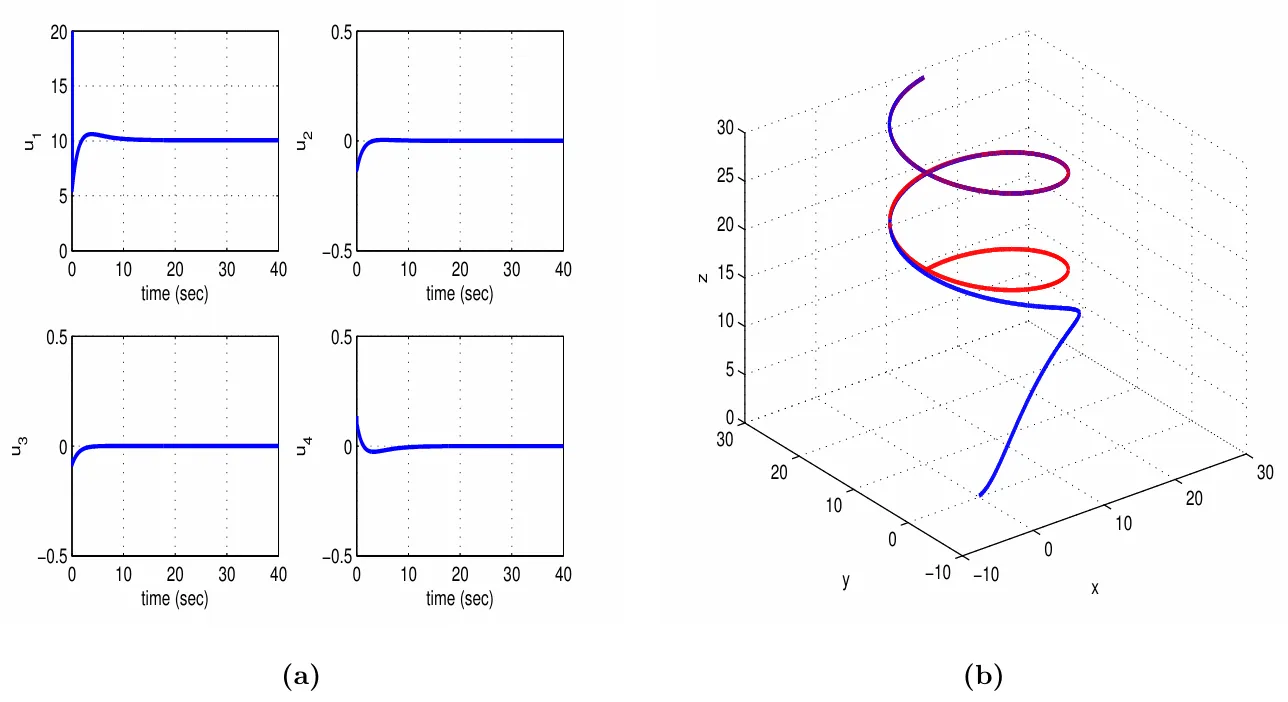
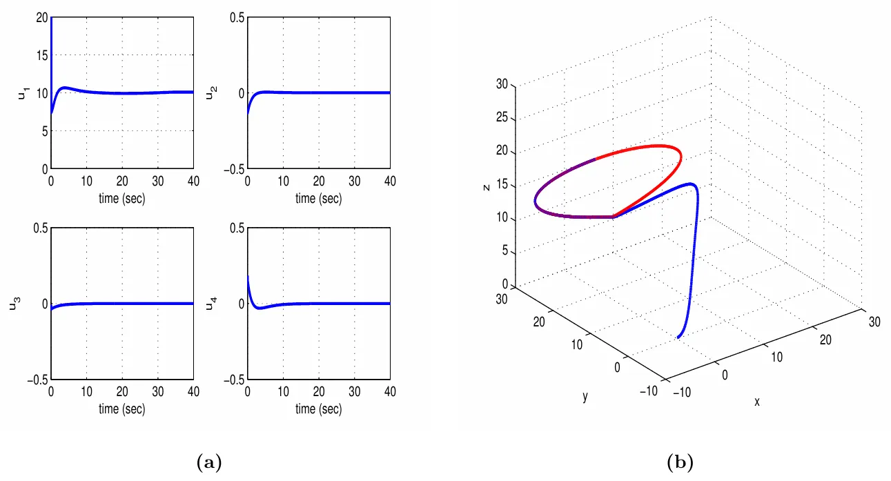
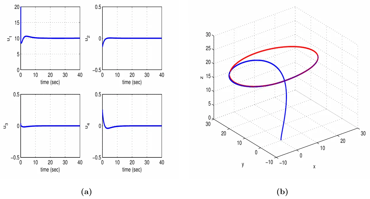
Figure 20. Tracking of setpoint 1 by the 6-DOF bicopter with the use of multi-loop flatness-based control: (<b>a</b>) variations of the control inputs u<sub>1</sub> and u<sub>4</sub> (blue lines) (<b>b</b>) convergence of the path of the bicopter’s center of gravity (blue line) to its reference trajectory in the XYZ cartesian space (red line).
Figure 21. Tracking of setpoint 2 by the 6-DOF bicopter with the use of multi-loop flatness-based control: (<b>a</b>) convergence of state variables x<sub>1</sub> to x<sub>6</sub> (blue lines) to the associated setpoints (red lines) and estimated values provided by Kalman Filtering (<b>b</b>) convergence of state variables x<sub>7</sub> to x<sub>12</sub> (blue lines) to the associated setpoints (red lines) and estimated values provided by Kalman Filtering.
Figure 22. Tracking of setpoint 2 by the 6-DOF bicopter with the use of multi-loop flatness-based control: (<b>a</b>) variations of the control inputs u<sub>1</sub> and u<sub>4</sub> (blue lines) (<b>b</b>) convergence of the path of the bicopter’s center of gravity (blue line) to its reference trajectory in the XYZ cartesian space (red line).
Figure 23. Tracking of setpoint 3 by the 6-DOF bicopter with the use of multi-loop flatness-based control: (<b>a</b>) convergence of state variables x<sub>1</sub> to x<sub>6</sub> (blue lines) to the associated setpoints (red lines) and estimated values provided by Kalman Filtering (<b>b</b>) convergence of state variables x<sub>7</sub> to x<sub>12</sub> (blue lines) to the associated setpoints (red lines) and estimated values provided by Kalman Filtering.
Figure 24. Tracking of setpoint 3 by the 6-DOF bicopter with the use of multi-loop flatness-based control: (<b>a</b>) variations of the control inputs u<sub>1</sub> and u<sub>4</sub> (blue lines) (<b>b</b>) convergence of the path of the bicopter’s center of gravity (blue line) to its reference trajectory in the XYZ cartesian space (red line).
Figure 25. Tracking of setpoint 4 by the 6-DOF bicopter with the use of multi-loop flatness-based control: (<b>a</b>) convergence of state variables x<sub>1</sub> to x<sub>6</sub> (blue lines) to the associated setpoints (red lines) and estimated values provided by Kalman Filtering (<b>b</b>) convergence of state variables x<sub>7</sub> to x<sub>12</sub> (blue lines) to the associated setpoints (red lines) and estimated values provided by Kalman Filtering.
Figure 26. Tracking of setpoint 4 by the 6-DOF bicopter with the use of multi-loop flatness-based control: (<b>a</b>) variations of the control inputs u<sub>1</sub> and u<sub>4</sub> (blue lines) (<b>b</b>) convergence of the path of the bicopter’s center of gravity (blue line) to its reference trajectory in the XYZ cartesian space (red line).
Figure 27. Tracking of setpoint 5 by the 6-DOF bicopter with the use of multi-loop flatness-based control: (<b>a</b>) convergence of state variables x<sub>1</sub> to x<sub>6</sub> (blue lines) to the associated setpoints (red lines) and estimated values provided by Kalman Filtering (<b>b</b>) convergence of state variables x<sub>7</sub> to x<sub>12</sub> (blue lines) to the associated setpoints (red lines) and estimated values provided by Kalman Filtering.
Figure 28. Tracking of setpoint 5 by the 6-DOF bicopter with the use of multi-loop flatness-based control: (<b>a</b>) variations of the control inputs u<sub>1</sub> and u<sub>4</sub> (blue lines) (<b>b</b>) convergence of the path of the bicopter’s center of gravity (blue line) to its reference trajectory in the XYZ cartesian space (red line).
Figure 29. Tracking of setpoint 6 by the 6-DOF bicopter with the use of multi-loop flatness-based control: (<b>a</b>) convergence of state variables x<sub>1</sub> to x<sub>6</sub> (blue lines) to the associated setpoints (red lines) and estimated values provided by Kalman Filtering (<b>b</b>) convergence of state variables x<sub>7</sub> to x<sub>12</sub> (blue lines) to the associated setpoints (red lines) and estimated values provided by Kalman Filtering.
Figure 30. Tracking of setpoint 6 by the 6-DOF bicopter with the use of multi-loop flatness-based control: (<b>a</b>) variations of the control inputs u<sub>1</sub> and u<sub>4</sub> (blue lines) (<b>b</b>) convergence of the path of the bicopter’s center of gravity (blue line) to its reference trajectory in the XYZ cartesian space (red line).
Figure 31. Tracking of setpoint 7 by the 6-DOF bicopter with the use of multi-loop flatness-based control: (<b>a</b>) convergence of state variables x<sub>1</sub> to x<sub>6</sub> (blue lines) to the associated setpoints (red lines) and estimated values provided by Kalman Filtering (<b>b</b>) convergence of state variables x<sub>7</sub> to x<sub>12</sub> (blue lines) to the associated setpoints (red lines) and estimated values provided by Kalman Filtering.
Figure 32. Tracking of setpoint 7 by the 6-DOF bicopter with the use of multi-loop flatness-based control: (<b>a</b>) variations of the control inputs u<sub>1</sub> and u<sub>4</sub> (blue lines) (<b>b</b>) convergence of the path of the bicopter’s center of gravity (blue line) to its reference trajectory in the XYZ cartesian space (red line).
Figure 33. Tracking of setpoint 8 by the 6-DOF bicopter with the use of multi-loop flatness-based control: (<b>a</b>) convergence of state variables x<sub>1</sub> to x<sub>6</sub> (blue lines) to the associated setpoints (red lines) and estimated values provided by Kalman Filtering (<b>b</b>) convergence of state variables x<sub>7</sub> to x<sub>12</sub> (blue lines) to the associated setpoints (red lines) and estimated values provided by Kalman Filtering.
Figure 34. Tracking of setpoint 8 by the 6-DOF bicopter with the use of multi-loop flatness-based control: (<b>a</b>) variations of the control inputs u<sub>1</sub> and u<sub>4</sub> (blue lines) (<b>b</b>) convergence of the path of the bicopter’s center of gravity (blue line) to its reference trajectory in the XYZ cartesian space (red line).
To elaborate on the tracking performance and on the robustness of the proposed multi-loop flatness-based control method for 6-DOF bicopter the following Tables are given: (i)
Table 4 which provides information about the accuracy of tracking of the reference setpoints by the state variables of the 6-DOF bicopter’s state-space model, (ii)
Table 5 which provides information about the robustness of the control method to parametric changes in the model of the 6-DOF bicopter, for instance change in mass $$m$$, (iii)
Table 6 which provides the convergence times of the 6-DOF bicopter’s state variables to the associated setpoints.
Table 4.
Multi-loop flatness-based control. Tracking RMSE for the 6-DOF bicopter in the disturbance-free case.
|
RMSEx1 |
RMSEx2 |
RMSEx3 |
RMSEx7 |
RMSEx8 |
RMSEx9 |
| setpoint1 |
0.0002 |
0.0001 |
0.0002 |
0.0001 |
0.0001 |
0.0001 |
| setpoint2 |
0.0009 |
0.0002 |
0.0005 |
0.0001 |
0.0001 |
0.0001 |
| setpoint3 |
0.0014 |
0.0003 |
0.0006 |
0.0001 |
0.0001 |
0.0001 |
| setpoint4 |
0.0009 |
0.0005 |
0.0014 |
0.0001 |
0.0001 |
0.0001 |
| setpoint5 |
0.0012 |
0.0002 |
0.0007 |
0.0001 |
0.0001 |
0.0001 |
| setpoint6 |
0.0004 |
0.0002 |
0.0009 |
0.0001 |
0.0001 |
0.0001 |
| setpoint7 |
0.0008 |
0.0003 |
0.0010 |
0.0001 |
0.0001 |
0.0001 |
| setpoint8 |
0.0002 |
0.0001 |
0.0002 |
0.0001 |
0.0001 |
0.0001 |
Table 5.
Multi-loop flatness-based control. Tracking RMSE for the 6-DOF bicopter in the case of disturbances.
| ∆a% |
RMSEx1 |
RMSEx2 |
RMSEx3 |
RMSEx7 |
RMSEx8 |
RMSEx9 |
| 0% |
0.0009 |
0.0005 |
0.0002 |
0.0001 |
0.0001 |
0.0001 |
| 10% |
0.0009 |
0.0002 |
0.0005 |
0.0001 |
0.0001 |
0.0001 |
| 20% |
0.0009 |
0.0002 |
0.0005 |
0.0001 |
0.0001 |
0.0001 |
| 30% |
0.0009 |
0.0002 |
0.0005 |
0.0001 |
0.0001 |
0.0001 |
| 40% |
0.0009 |
0.0002 |
0.0005 |
0.0001 |
0.0001 |
0.0001 |
| 50% |
0.0010 |
0.0002 |
0.0005 |
0.0001 |
0.0001 |
0.0001 |
| 60% |
0.0010 |
0.0002 |
0.0006 |
0.0001 |
0.0001 |
0.0001 |
Table 6.
Multi-loop flatness-based control. Convergence time (s) for the 6-DOF bicopter.
|
Ts x1 |
Ts x2 |
Ts x3 |
Ts x7 |
Ts x8 |
Ts x9 |
| setpoint1 |
7.5 |
7.5 |
8.0 |
12.0 |
7.5 |
2.5 |
| setpoint2 |
8.0 |
7.5 |
10.0 |
12.5 |
7.5 |
2.5 |
| setpoint3 |
0.5 |
0.5 |
8.0 |
12.5 |
7.5 |
2.5 |
| setpoint4 |
8.0 |
8.0 |
0.5 |
12.5 |
7.5 |
2.0 |
| setpoint5 |
0.5 |
0.5 |
10.0 |
12.5 |
7.5 |
7.5 |
| setpoint6 |
7.5 |
7.5 |
10.0 |
12.5 |
7.5 |
7.5 |
| setpoint7 |
10.0 |
8.0 |
9.0 |
12.5 |
7.5 |
7.5 |
| setpoint8 |
9.0 |
8.0 |
8.0 |
12.5 |
7.5 |
7.5 |
10. Conclusions
The article has proposed two different solutions for the nonlinear control problem of the 6-DOF bicopter: (i) nonlinear optimal control, (ii) multi-loop flatness-based control. In (i) nonlinear optimal control the dynamic model of the 6-DOF bicopter undergoes linearization at each sampling instance around the temporary operating point $$\left( x^{∗} , u^{∗} \right)$$ where $$x^{∗}$$ is the present value of the drone’s state vector and $$u^{∗}$$ is the last sampled value of the control inputs vector. The linearization is based on Taylor series expansion and on the computation of Jacobian matrices. For the linearized model of the system an H-infinity feedback controller is designed. The H-infinity controller represents a min-max differential game where the control inputs try to minimize a cost function which contains a quadratic term of the state vector’s tracking error while the model uncertainty and external perturbation terms try to maximize this cost function. To compute the feedback gains of this controller an algebraic Riccati equation is solved repetitively at each time-step of the control algorithm. The global stability properties of the control scheme are proven through Lyapunov analysis. The nonlinear optimal control approach assures fast and accurate tracing of setpoints by the state variables of the 6-DOF bicopter, while also keeping moderate the variations of the control inputs.
At a second stage the article has examined a multi-loop flaatness-based control method for the dynamic model of the 6-DOF bicopter. The drone’s dynamics is written in the form of two chained and differentially flat subsystems. The state vector of the second subsystem becomes virtual control input to the first subsystem, while the control inputs of the first subsystem become setpoints for the second subsystem. Knowing that differential flatness properties hold for each one of these subsystems a stabilizing feedback controller can be designed for each one of them by inverting their dynamics as it is commonly done for input-output linearized flat systems. The global stability properties of the multi-loop flatness-based control scheme are proven though Lyapunov analysis. Multi-loop flatness-based control achieves precise tracking of setpoints by the state variables of the 6-DOF bicopter without the need for changes of state variables or state-space model transformations.
Author Contributions
Conceptualization: G.R., P.S., M.A., Z.G., L.D. and M.A.-N., Methodology: G.R., Software: G.R., Validation: G.R., P.S., M.A., Z.G., L.D. and M.A.-N., Formal Analysis: G.R., P.S., M.A., Z.G., L.D. and M.A.-N., Investigation: G.R., Resources: G.R., P.S. and M.A.-N., Data Curation: N/A, Writing—Original Draft Preparation: G.R., Writing—Review & Editing: G.R., Visualization: G.R., Supervision: G.R., Project Administration: G.R., Funding Acquisition: G.R., P.S. and M.A.-N.
Ethics Statement
Not Applicable.
Informed Consent Statement
Not Applicable.
Data Availability Statement
Data about the article's experimental results are available from the authors upon reasonable request.
Funding
(a) Gerasimos Rigatos has been partially supported by Grant Ref. 040723 “Autonomous electric vehicles: Nonlinear control, traction and propulsion” of the Unit of Industrial Automation, Industrial Systems Institute, Greece (b) Pierluigi Siano and Mohammed Al-Numay acknowledge financial support from the Researchers Supporting Project Number (RSP2025R150), King Saud University, Riyadh, Saudi Arabia.
Declaration of Competing Interest
The authors declare that, to their knowledge, no conflict exists with third parties about the content and developments of this article.
References
-
1.
Qin Y, Chen N, Cai Y, Xu W, Zhang F. Gemini II: Design, modeling and control of a compact yet efficient servoless bicopter.
IEEE/ASME Trans. Mechatron. 2022,
27, 4304–4315.
[Google Scholar]
-
2.
Li S, Liu F, Gao Y, Xiang J, Tu Z, Li D. AirTwins: Modular bicopters capable of splitting from their combined quadropter in midair.
IEEE Robot. Autom. Lett. 2023,
8, 6068–6075.
[Google Scholar]
-
3.
Zhao H, Zi R, Quan Q. Relaxed hover solution-based control for a bicopter with rotor and servo stuck failure. In Proceedings of the 2024 IEEE International Conference on Robotics and Automation (ICRA), Yokohama, Japan, 13–17 May 2024.
-
4.
Fahmizal, Nagrado HA, Cahyadi AJ, Ardiyanto I. Attitude control of UAV bicopter using adaptive LQG.
Results Control. Optim. 2024,
17, 100484.
[Google Scholar]
-
5.
Abedini A, Bataleblu A, Roshanian J. Codesign optimization of a novel multi-identity drone helicopter (MICOPTER).
J. Intell. Robot. Syst. 2022,
106, 56.
[Google Scholar]
-
6.
Abedini A, Bataleblu A, Roshanian J. Robust backstepping control of position and attitude for a bicopter drone. In Proceedings of the 2021 9th RSI International Conference on Robotics and Mechatronics (ICRoM), Tehran, Iran, 17–19 November 2021.
-
7.
Ding J, Zhu Y, Zhang L, Dong Y, Ding Y. Sytab: A class of smooth transition hybrid terrestrial / aerial bicopters.
IEEE Robot. Autom. Lett. 2022,
7, 9199–9206.
[Google Scholar]
-
8.
Li Y, Qin Y, Xu W, Zhang F. Modeling, identification and control of non-minimum phase dynamics of bicopter UAVs. In Proceedings of the 2020 IEEE/ASME International Conference on Advanced Intelligent Mechatronics (AIM), Boston, MA, USA, 6–9 July 2020.
-
9.
Marton LT, Kutasi DN. Modeling and Control Strategies For Bicopter Type UAVs. In Proceedings of the 2024 25th International Carpathian Control Conference (ICCC), Krynica Zdrój, Poland, 22–24 May 2024.
-
10.
Xu Y, Gao L, Liu B, Zhang J, Zhu Y, Zhao J. Analysis and control of an active balance tail for the tilting dual-rotor UAV.
Aircr. Eng. Aerosp. Technol. 2024,
96, 1192–1202.
[Google Scholar]
-
11.
Anzai T, Kojia Y, Makabe T, Okada K, Inaba M. Design and development of a flying humanoid robot platform with bicopter flight units. In Proceedings of the 2020 IEEE-RAS 20th International Conference on Humanoid Robots (Humanoids), Munich, Germany, 19–21 July 2021.
-
12.
Zhang Q, Liu Z, Zhao J, Zhang S. Modeling and attitude control of bicopters. In Proceedings of the 2016 IEEE International Conference on Aircraft Utility Systems (AUS), Beijing, China, 10–12 October 2016.
-
13.
He X, Wang Y. Design and trajectory tracking control of a new bicopter UAV.
IEEE Robot. Autom. Lett. 2022,
7, 9191–9198.
[Google Scholar]
-
14.
Portella Delgado J.M, Goel A. Adaptive nonlinear control of a bicopter with unknown dynamics. In Proceedings of the 2024 American Control Conference, Toronto, ON, Canada, 10–12 July 2024.
-
15.
Bertrand S, Hamel T, Piet-Lahanier H. Stability analysis of an UAV controller using perturbation theory. In Proceedings of the IFAC WC 2008, 17th World Congress of the Intl. Federation on Automatic Control, Seoul, Korea, 6–11 July 2008.
-
16.
Darvispoor S, Roshanian J, Tayefi M. A novel concept of VTOL birotor UAV based on moving mass control.
Aerosp. Sci. Technol. 2020,
107, 106238.
[Google Scholar]
-
17.
Aschemann H, Meinlschmidt T. Cascaded nonlinear control of a duocopter with disturbance compensation by an Unscented Kalman Filter. In Proceedings of the IMACS Mathmod 2015, 8th Vienna International Conference on Mathematical Modelling, Vienna, Austria, 18–20 February 2015.
-
18.
Abedini A, Bataleblu A, Roshanian J. Robust trajectory tracking for a bicopter drone using IBKS and SPNN adaptive controllers. In Proceedings of the 2022 10th RSI International Conference on Robotics and Mechatronics (ICRoM), Tehran, Iran, 22–24 November 2022.
-
19.
Amir N, Ramirez-Serrano A, Davies RJ. Integral backstepping control of an unconventional dual-fan unmanned aerial vehicle.
J. Intell. Robot. Syst. 2013,
69, 147–159.
[Google Scholar]
-
20.
Meinschmidt T, Aschemann H. Cascaded flatness-based control of a duocopter subject to unknown disturbances. In Proceedings of the 2014 19th International Conference on Methods and Models in Automation and Robotics (MMAR), Miedzyzdroje, Poland, 2–5 September 2014.
-
21.
Aschemann H. Robust control of a duocopter by discrete-time sliding-mode technique and an Extended Kalman Filter for disturbance compensation. In Proceedings of the 2022 26th International Conference on Methods and Models in Automation and Robotics (MMAR), Myedzyzdroje, Poland, 22–25 August 2022.
-
22.
Yang CM, Bhounsule PA. Robust control using control Lyapunov function and Hamilton-Jacobi reachability. In Proceedings of the IFAC 4th Modeling, Estimation and Control Conference, Chicago, IL, USA, 28–30 October 2024.
-
23.
Meinlschmidt T, Aschemann H, Bart SS. Cascaded backstepping control of a duocopter including disturbance compensation by Unscented Kalman Filtering. In Proceedings of the 2014 International Conference on Control, Decision and Information Technologies (CoDIT), Metz, France, 3–5 November 2014.
-
24.
Aschemann H, Prabel R. Robust disturbance compensation for a duocopter by gain-scheduled nonlinear control and observer design. In Proceedings of the IECON 2015–41st Annual Conference of the IEEE Industrial Electronics Society, Yokohama, Japan, 9–12 November 2015.
-
25.
Ahmed F, Sobiesiak L, Forbes JR. Model Predictive Control of a Tandem-Rotor Helicopter With a Nonuniformly Spaced Prediction Horizon.
IEEE Control Syst. Lett. 2022,
6, 2828–2833.
[Google Scholar]
-
26.
Li W, Yang P, Geng K, Zhu X. Fault-tolerant attitude tracking control of tandem rotor helicopter considering internal actuator saturation and external wind gust.
Int. J. Adapt. Control Signal Process. 2023,
37, 1671-1692.
[Google Scholar]
-
27.
Duan D, Li Y, Ding Z, Li J. Flight dynamics analysis of a small tandem helicopter considering aerodynamic interference.
Proc. IMechE Part G J. Aerosp. Eng. 2022,
236, 2803–2816.
[Google Scholar]
-
28.
Xu X, Watanabe K, Nagai I. Feedback linearization control for a tandem rotor UAV robot equipped with two 2‑DOF tiltable coaxial‑rotors.
Artif. Life Robot. 2021,
26, 259–268.
[Google Scholar]
-
29.
Ahmed F, Sobiesiak L, Forbes JR. Cascaded Model Predictive Control of a Tandem-Rotor Helicopter.
IEEE Control Syst. Lett. 2023,
7, 1345–1350.
[Google Scholar]
-
30.
Rigatos G, Busawon K. Robotic Manipulators and Vehicles: Control, Estimation and Filtering; Springer: Cham, Switzerland, 2018.
-
31.
Rigatos G, Karapanou E. Advances in Applied Nonlinear Optimal Control; Cambridge Scholars Publishing: Newcastle upon Tyne, UK, 2020.
-
32.
Rigatos G, Abbaszadeh M, Siano P. Nonlinear Optimal and Flatness-Based Control Methods and Applications for Complex Dynamical Systems; IET Publications: London, UK, 2025.
-
33.
Rigatos G, Abbaszadeh M, Siano P. Control and Estimation of Dynamical Nonlinear and Partial Differential Equation Systems: Theory and Applications; IET Publications: London, UK, 2022.
-
34.
Rigatos G. Nonlinear Control and Filtering Using Differential Flatnesss Theory Approaches: Applications to Electromechanical Systems; Springer: Cham, Switzerland, 2015.
-
35.
Rigatos GG, Tzafestas SG. Extended Kalman Filtering for Fuzzy Modelling and Multi-Sensor Fusion, Mathematical and Computer Modelling of Dynamical Systems.
Math. Comput. Model. Dyn. Syst. 2007,
13, 251–266.
[Google Scholar]
-
36.
Basseville M, Nikiforov I. Detection of Abrupt Changes: Theory and Applications; Prentice-Hall: Hoboken, NJ, USA, 1993.
-
37.
Rigatos G, Zhang Q. Fuzzy model validation using the local statistical approach.
Fuzzy Sets Syst. 2009,
60, 882–904.
[Google Scholar]
-
38.
Toussaint GJ, Basar T, Bullo F. 𝐻∞ optimal tracking control techniques for nonlinear underactuated systems. In Proceedings of the IEEE CDC 2000, 39th IEEE Conference on Decision and Control, Sydney, Australia, 12–15 December 2000.
-
39.
Rigatos G, Abbaszadeh M, Siano P, Wira P. Autonomous Electric Vehicles: Nonlinear Control, Traction and Propulsion; Elsevier: Amsterdam, The Netherlands, 2024.
-
40.
Rigatos G, Abbaszadeh M, Hamida MA, Siano P. Intelligent Control for Electric Power Systems and Electric Vehicles; CRC Publications: Boca Raton, FL, USA, 2024.