
A Method for Predicting the Crystallinity of Linear and Branched Polyethylene †
A Method for Predicting the Crystallinity of Linear and Branched Polyethylene †

Received: 23 July 2026 Revised: 17 August 2026 Accepted: 26 August 2026 Published: 20 September 2026

© 2026 The authors. This is an open access article under the Creative Commons Attribution 4.0 International License (https://creativecommons.org/licenses/by/4.0/).
1. Introduction
Tailoring product properties for industrial applications is a crucial issue in chemical engineering. When dealing with polymers, the crystallinity in particular has a major impact on physical properties such as gas solubility, melting behavior, and tensile strength [1]. The crystallinity itself depends mainly on the structure of polyethylene [2], in which backbone branching, including short and long chains, plays a major role [1,3,4].
Flory [5] was the first to develop a physical relationship (FCA) between the branching degree, the temperature, and the crystallinity of polymers. He considered a branched polyethylene as a copolymer, with only one type of monomer being crystallizable. While capturing the general dependencies of decreasing crystallinity with increasing branching degree, the main drawback is the description of the linear unbranched polymer, since Flory’s theory [5] gives 100% for the limiting crystallinity. However, experiments have shown that unbranched polyethylene in fact does not crystallize completely [6,7]. There are mainly two reasons for the reduced crystallinity of linear polymers. A polymer melt consists of twisted, looped, and knotted chains. These entanglements do not suddenly detangle shortly before crystallization; instead, they remain in the amorphous phase as non-crystallizable units, thereby lowering the overall crystallinity [8]. Second, as crystallization progresses, certain polymer chain sequences become isolated and are too short to form a stable crystallite, thereby remaining amorphous as well [8]. While chain entanglement is an issue widely discussed in literature [6,9,10,11,12,13,14], only a few have dealt with the issue of isolated, hence wasted space, during crystallization [15,16,17,18].
One way to determine the wasted space that emerges as crystallization progresses is based on the figurative problem of cars being randomly placed along a curb without overlapping, also known as the Car-Parking-Problem (CPP) [19]. While this approach was applied successfully in the field of adsorption [20,21,22,23], it found barely any attention in the field of crystallization. Gornick and Jackson [16] transferred the CPP to the crystallinity of polymer chains by calculating the wasted space that evolves between two sequences that have already crystallized but are too short to form another stable crystallite. Maltz and Mola [17,24] introduced another point of view by considering the crystallization as a continuous process in which the sequences crystallize one after another, resulting in different probabilities for different configurations. Independent from Maltz and Mola’s extension [17,24], Gornick and Freedman [25] derived the same relations 10 years later. Yet, both the statistical and the continuous approaches were introduced at a merely academic level and, according to our knowledge, have not been further investigated.
In this work, a framework is presented that accounts for the crystallinity of linear polyethylene by incorporating the CPP both in a purely statistical manner and continuously. Afterward, branching is incorporated by considering the polyethylene as a copolymer. Finally, predictions for the crystallinity of both linear and branched polyethylene are presented and compared with experimental data taken from the literature [9,26,27,28,29,30,31,32,33,34,35,36,37,38,39,40,41,42,43,44,45,46,47,48,49,50] covering a wide range of molecular weight, temperature, and branching.
2. Theoretical Framework
For the general treatment of crystallinity, polymer configurations are accommodated in a lattice [51]. In this context, a crystalline region is characterized by $${\zeta }^{*}$$, the equilibrium number of repeating structural elements of one chain, which in the case of polyethylene is $$C{H}_{2}$$-segments. The crystallinity, $${\alpha }^{lin},$$ of the linear polyethylene is then defined as:
where $${j}_{max}$$ is the maximal number of crystalline sequences, and $$M$$ is the segment number of the entire chain. The segment number is given directly by the molecular weight divided by the molar mass of a segment. However, $${\zeta }^{*}$$ and $${j}_{max}$$ are unknown. For this reason, the former considers the free energy change in forming a crystallite, while for $${j}_{max}$$ the car-parking problem is applied to polymer crystallization.
2.1. Crystalline Sequence Length
Based on the works of Flory [51], Mandelkern et al. [52] found an implicit expression for the free energy change $$\mathrm{\Delta }F$$ in forming a crystallite:
where $$\zeta$$ is the crystalline sequence length, differing from the crystalline sequence length $${\zeta }^{*}$$ in equilibrium. $$\rho$$ is the number of cylindrically arranged crystalline sequences in cross section, $$N$$ is the number of polymer chains, $$M$$ is the segment number, $$T$$ is the system temperature, $${\mathrm{\Delta }}_{SL}h$$ is the melting enthalpy of one segment, $${T}_{0}^{SL}$$ is the melting temperature, and $${\sigma }_{u}$$ is the lateral surface free energy of a chain. The second term in the squared brackets of Equation (2) has a different sign compared to the publication [52], which is, however, in agreement with [51,53]. In this work, $${\mathrm{\Delta }}_{SL}h$$ is divided by 2 as it refers to one ethylene-unit, which contains two segments. $$D$$ in Equation (2) which is regarded by Flory [51] and Mandelkern et al. [52] as the nucleation constant, is defined as follows:
whereby $${\sigma }_{e}$$ is the surface energy and $${a}_{0}$$ the cross-sectional area of the polymer chain. With the help of the first term of a Taylor series expansion, the first term of Equation (2) in squared brackets $$N\mathrm{ln}\left(1 -\frac{\zeta \rho }{NM}\right)$$ can be written as $$-\zeta \rho /M$$. Strictly speaking, this is only valid at small crystallinities. However, the error should be minor compared to the general inaccuracies involved in dealing with crystallinities. $$\mathrm{\Delta }F$$ in Equation (2) does not exhibit a maximum or minimum, but shows a saddle point where the free energy derivatives $${\left(\frac{\partial \mathrm{\Delta }F}{\partial \zeta }\right)}_{\rho }$$ and $${\left(\frac{\partial \mathrm{\Delta }F}{\partial \rho }\right)}_{\zeta }$$ equal zero [52]. Combining both derivatives leads to the crystalline sequence length in equilibrium, $${\zeta }^{*}$$:
whereby $${\sigma }_{u}$$ vanishes. While $${\mathrm{\Delta }}_{SL}h$$ and $${T}_{0}^{SL}$$ are substance properties, which are experimentally accessible, $${\sigma }_{e}$$ in Equation (3) is a property coming from crystallization growth kinetics, whose estimation is accompanied by larger uncertainties. For lower molecular weights, there is probably an effect of the chain length on $${\sigma }_{e}$$ [54] which will be disregarded here for the sake of simplification. However, the impact of $${\sigma }_{e}$$ on the calculation results are rather small. Parameters for Equation (3) and Equation (4) are given in Table 1. By using Equation (3) in combination with Equation (4), $${\zeta }^{*}$$ can be calculated.
Table 1. Parameters used for the model predictions Equation (3) and Equation (4).
|
Quantity |
Value |
Method |
Ref. |
|---|---|---|---|
|
$${\mathrm{\Delta }}_{SL}h \left[\mathrm{k}\mathrm{J}/\mathrm{m}\mathrm{o}{\mathrm{l}}_{{\mathrm{C}}_{2}{\mathrm{H}}_{4}}\right]$$ |
$$8.284$$ |
(a) |
[55] |
|
$${T}_{0}^{SL} \left[\mathrm{K}\right]$$ |
$$414.6$$ |
(b) |
[56] |
|
$${a}_{0} \left[{\mathrm{m}}^{2}/\mathrm{m}\mathrm{o}\mathrm{l}\right]$$ |
$$1.1\times {10}^{5}$$ |
- |
[57] |
|
$${\sigma }_{e} \left[\mathrm{m}\mathrm{J}/{\mathrm{m}}^{2}\right]$$ |
168 |
(c) |
[58] |
(a): Differential Scanning Calorimetry with solution-grown crystals of orthorhombic phase, (b): extrapolation of linear chain homologs, (c): nucleation kinetics of polyethylene droplets.
2.2. Car-Parking-Problem
After determining $${\mathrm{\zeta }}^{\mathrm{*}}$$ (Equation (4)), $${j}_{max}$$ is required for calculating the crystallinity according to Equation (1). This is done via the car-parking-problem (Figure 1a), which was constructed by Renyi in 1958 [19]. In this 1-dimensional random space-filling problem, the following question was posed: Having a given interval $$\left(0,x\right)$$, how many units $$j$$, which have the length 1, can be placed so that no points overlap. The question is similar to the illustration of identical cars, randomly parked along a curb, which is why the problem is known as the car-parking problem. Renyi [19] postulated the following continuous recursion for the number of $$j$$, that can be placed on $$\left(0,x\right)$$, while $$j$$ has the length 1:
Forming the limit of the unit density $$j\left(x\right)/x$$ for an infinite interval, one obtains the famous car-parking-constant $$C$$:
2.3. Statistical Treatment
Gornick and Jackson [16] applied the car-parking-problem to the crystallization of polymers by considering a polyethylene chain consisting of $$M$$ segments in which $$j$$ sequences of length $${\zeta }^{*}$$ are crystallized (Figure 1b). For the calculation of $${j}_{max}$$, the wasted space $$W$$ is required, e.g., the remaining amorphous sequences which are too short to accommodate another crystalline sequence. One obtains $$W$$ with the following expression [16]:
whereby $$r$$ is the length of an amorphous interval and $$P\left(r\right)$$ is the probability that an amorphous interval has this length. Wasted space is produced if intervals are too small to accommodate a crystalline sequence, which means $$r<{\mathrm{\zeta }}^{\mathrm{*}}$$, causing the sum in Equation (7) to run to $${\zeta }^{*}-1$$. The factor $$j+1$$ in Equation (7) results from the reference to the entire chain. Technically speaking, there are configurations of $$P\left(r\right)$$, where less intervals than $$j+1$$ exist, due to crystalline sequences placed directly adjacent to each other. In this case, the factor $$j+1$$ in Equation (7) is replaced by $$j$$. However, for long chains this effect is negligible. Equation (7) is valid if enough amorphous segments $$A$$ remain so the sum can reach the value $${\zeta }^{*}-1$$, whereby $$A$$ is given by:
There is one exception to Equation (7), which is introduced in this work: In the case of high crystallinities, the number of amorphous segments $$A$$ may be too small to accommodate another crystalline sequence. In this case, all the amorphous segments become wasted space, which leads to the following expression:
Subsequently, for the calculation of the wasted space with Equation (7), an expression for $$P\left(r\right)$$ is required. This is achieved by considering $$N\left(M,j,{\zeta }^{*}\right)$$, the number of possibilities, arranging $$j$$ sequences in a polymer chain consisting of $$M$$ segments and crystalline sequences having the length $${\zeta }^{*}$$. In other words, $$N\left(M,j,{\zeta }^{*}\right)$$ is the number of permutations of $$j$$ crystalline sequences with $$A$$ amorphous segments (Equation (8)), given by the following expression [16]:
With the help of Equation (10), $$P\left(r\right)$$ can be calculated [16]:
Gornick and Jackson [16] determined the limiting case of Equation (11) for $$M\to \infty$$, $$j\to \infty$$ and large $${\zeta }^{*}$$, in order to solve Equation (11) analytically. With this, they were able to successfully account for combinatorial limitations of the crystallinity. Unfortunately, only polymer chains of infinite length can be considered. In contrast, in this work, Equation (11) is solved for the first time for a finite number of segments. Since the calculation of faculties for high segment numbers is extremely CPU-intensive, Equation (11) is approximated with the help of Stirling’s formula:
Using Equation (11) and Equation (12) result in the following equation:
Now, the wasted space can be calculated as a function of $$M$$, $${\zeta }^{*}$$ and $$j$$ with the help of Equation (7) and Equation (9). Yet, to obtain the crystallinity (Equation (1)), the maximal number of crystalline sequences $${j}_{max}$$ is required. This is achieved in this work by calculating the derivative of $$W$$ (given by Equation (7) and Equation (9)) according to $$j$$, which is then set to zero:
Therefore, by solving Equation (14), $${j}_{max}$$ can be obtained, and the derivation can be calculated using Equation (13), which results in:
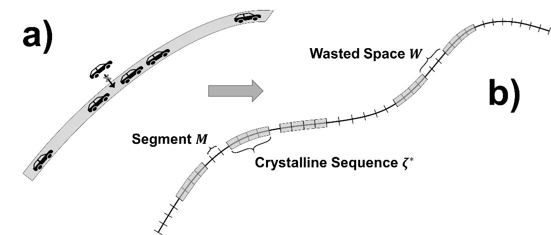
Figure 1. (a) Model concept of the car-parking-problem. (b) Application to crystallization of a polymer chain.
2.4. Continuous Filling
While the approach of Gornick and Jackson [16] is a purely statistical consideration of the problem, Maltz and Mola [17,24] introduced a continuous view of the problem. In this approach, the chronology of the crystalline sequences comes into play, which is elucidated in Figure 2.
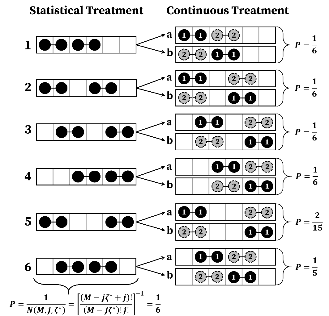
Figure 2. Probability $$P$$ of filling two 2-segment-sequences into a compartment of six segments. On the left-hand side is the purely statistical approach. On the right-hand side is the continuous treatment: First, a black sequence is inserted, followed by a grey sequence.
For the left-hand side of Figure 2, Equation (10) can be applied, resulting in a probability of $$1/6$$ for one of the possible arrangements 1/6. For the calculation of the right-hand side, one has to calculate the possibility of the black sequence to find its place in an empty compartment, which is $$1/5$$ in all configurations. The probability of introducing the grey sequence into 1a is $$1/3$$, respectively $$1/2$$ for 1b, resulting in an overall probability of configuration 1 of $$P=1/5\cdot 1/3+1/5\cdot 1/2=1/6$$. The same accounts for configurations 2–4 in Figure 2. However, configurations 5 and 6 in Figure 2 equal a probability of $$2/15$$, respectively $$1/5$$.
For calculating the wasted space, two natural constraints must be considered [17,24]. If the crystalline sequence length $${\zeta }^{*}$$ is larger than the length of the polymer chain $$M$$, all space is wasted.
Secondly, if $${\zeta }^{*}$$ equals the chain length, however improbable, the whole chain crystallizes at once, resulting in a wasted space of zero [17]:
The recursive formulism in case $${\zeta }^{*}$$ is smaller than $$M$$ is as follows [17]:
The crystallinity of the continuous approach is obtained by using the last value of the recursive formula of $$W$$ (Equation (18)) and Equation (19). In this case, Equation (1) is replaced by:
Freedman and Gornick [59] addressed the same issue 10 years later and reached the same result (Equation (18) and Equation (19)) independently of Maltz and Mola [17,24]. Both methods can only be applied to linear chains.
2.5. Branching
In case of branched chains, the degree of branching $$br$$ must be incorporated. A fundamental predictive model for estimating the crystallinity, $${\alpha }^{br}$$, as a function of the branching degree $$br$$ was introduced by Flory [5], where $$br$$ is the number of threefold branching points per 1000 carbon atoms, since polyethylene exhibits almost exclusively threefold branching points. As can be seen in Figure 3, the polymer chain is divided into units A (main chain) and units Co (co-monomer), with just A-units being crystallizable. The co-monomer represents the branching. This limitation means that maybe the model can not be applied to very long branches.
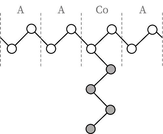
With the help of the branching degree $$br$$ and the number of segments in the branch $${n}_{br}$$ (grey circles in Figure 3), the mole fraction of A units $${x}_{A}$$ for random copolymers is calculated [5]:
The volume fraction of A-units $${\phi }_{A}$$ differs from the mole fraction $${X}_{A}$$, since monomers A and Co do not have the same volume:
The crystallinity of branched polyethylene is given by [5]:
$$\theta$$ in Equation (22) is calculated as follows:
where $${\mathrm{\Delta }}_{SL}h$$ is the melting enthalpy of one A-unit and $${T}_{0}^{SL}$$ the melting temperature of the unbranched linear chain. The same parameters for $${\mathrm{\Delta }}_{SL}h$$ and $${T}_{0}^{SL}$$ are used for the calculation of the linear crystalline sequence length given in Table 1. The second term in the denominator of Equation (22) differs from Flory’s original approach [5]. This correction was shown by Kilian [60], Baur [61], and Wunderlich [62] and considers the fact that only amorphous sequences are available for further crystallization. The critical crystalline length $${\zeta }_{cr}$$ is calculated as follows:
which is a function of the temperature, expressed by $$\theta$$ (Equation (23)). $$D$$ is given by Equation (3). Solely sequences composed of A-units that are at least equivalent to $${\zeta }_{cr}$$ can crystallize. $${\zeta }_{cr}$$ should not be confused with $${\zeta }^{*}$$, accounting for the merely linear chain.
2.6. Numerical Procedure
The numerical procedure for the prediction of crystallinities is shown in Figure 4. First, the crystalline sequence length $${\zeta }^{*}$$ is calculated via Equation (4). Afterward, the limiting crystallinity for a linear polyethylene chain via the CPP is predicted with Equation (1) or Equation (19) and the crystallinity of the branched chain prescribed by the FCA using Equation (22). The final crystallinity $$\alpha$$ is assumed to be $${\alpha }^{lin}\cdot {\alpha }^{br}$$.
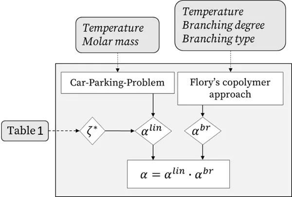
Figure 4. Numerical procedure for prediction of the crystallinity of polyethylene with the CPP/FCA. Rectangles with rounded corners are input variables, and diamonds are calculations.
3. Results and Discussions
3.1. Linear Polyethylene
Figure 5 shows both experimental data of electron microscope studies [63,64] and predictions of $${\zeta }^{*}$$ for the linear chain as a function of the segment number $$M$$ for different temperatures.
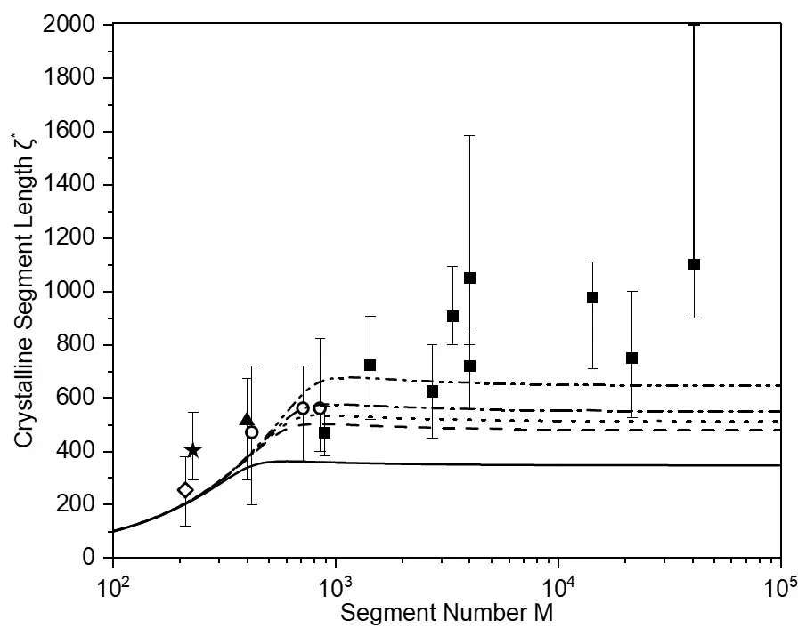
Figure 5. Plot of $${\zeta }^{*}$$ as a function of $$M$$, calculated with Equation (4) for different temperatures. Parameters taken from Table 1. Experimental data from Mandelkern [63] (filled symbols) and Anderson [64] (open symbols) for $$T=393.15 \,\mathrm{K}$$ (solid line, diamonds), $$T=399.15\, \mathrm{K}$$ (dashed line, stars), $$T=400.15 \,\mathrm{K}$$ (dotted line, triangles), $$T=401.15\, \mathrm{K}$$ (dashed-dotted line, circles) and $$T=403.15 \,\mathrm{K}$$ (dashed double dotted line, squares), where bars represent the range of the electron microscope studies while the symbols depict the mean value.
The quantity $${\zeta }^{*}$$ as a function of the segment-number, respectively molecular weight, has two characteristic parts: first, for low molecular weights, $${\zeta }^{*}$$ is independent of the temperature and has almost linear growth. In this area, $${\zeta }^{*}$$ corresponds roughly to the chain length. Second, for higher molecular weights, $${\zeta }^{*}$$ levels off and is almost independent of the molecular weight. The value for $${\zeta }^{*}$$ is approximately given by the limit of Equation (4) being $$\underset{M\to \infty }{\mathrm{lim}}{\zeta }^{*}=8{\sigma }_{e}a{T}_{0}^{SL}/\left({\mathrm{\Delta }}_{SL}h\left({T}_{0}^{SL}-T\right)\right)$$. The calculations reproduce the experimental data qualitatively, considering the experimental inaccuracies.
Applying the purely statistical approach (Equation (7) and Equation (9)), one can calculate the wasted space as a function of the crystallinity for different crystalline sequence lengths, which is shown in Figure 6. Coming from low crystallinities, $$W$$ increases slowly at first and drops after a maximum to 0. The wasted space cannot decrease with increasing crystallinity, hence $$\frac{\partial W}{\partial \alpha }$$ must be positive in the physically useful range. This is why the maximum in $$W$$ simultaneously represents the maximal accessible amount of crystallinity and therefore the maximal number of crystalline sequences, $${j}_{max}$$. This value of $${j}_{max}$$ is calculated by solving Equation (14) and shown as stars in Figure 6. For high crystallinities, the crystallinity is prescribed by Equation (9), where all remaining amorphous segments become wasted space, which is represented by the bold line in Figure 6.
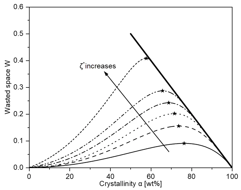
Figure 6. Wasted space as a function of the crystallinity $$\alpha$$ for different crystalline sequence lengths $${\zeta }^{*}$$ at a constant chain length of $$M=1\times {10}^{5}$$. Solid line: $${\zeta }^{*}=2$$, dashed line: $${\zeta }^{*}=5$$, dotted line: $${\zeta }^{*}=100$$, dash-dotted line: $${\zeta }^{*}=10,000$$, dashed double dotted line: $${\zeta }^{*}=20,000$$, short dashed line: $${\zeta }^{*}=40,000$$ calculated with Equation (7). The stars denote the maximal reachable crystallinity calculated with Equation (14). The bold line denotes the wasted space via Equation (9).
Figure 7 shows the maximal crystallinity, calculated with Equation (9), as a function of the $${\zeta }^{*}$$, which equals the crystallinity of the maximum of the wasted space in Figure 6 (stars), calculated with Equation (14). Additionally, Figure 7 shows the wasted space $$W$$ of a single crystalline sequence (which can be obtained by inserting $$j=1\,$$in Equation (9)) as well as the corresponding crystallinity of a single crystalline sequence (which can be obtained by inserting $$j=1\,$$in Equation (1)). The maximal crystallinity in Figure 7, coming from the left side, e.g., at low crystalline sequence lengths, reaches a plateau at approx. $$71 \%$$ after an initial decrease, before it decreases again and finds its minimum at $$50\%$$. From $${\zeta }^{*}/M=0.5$$ on, the crystallinity increases again since it is prescribed by the crystallinity for a chain having a single crystalline sequence.
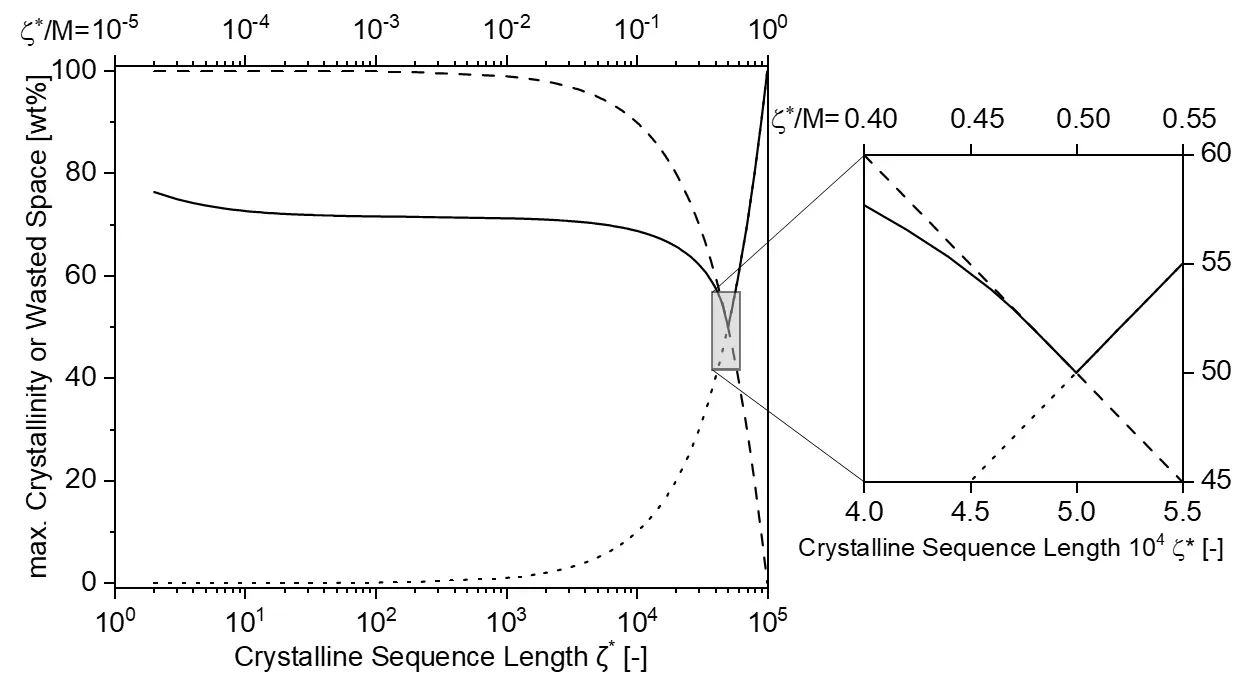
Figure 7. The solid line shows the maximal crystallinity as a function of $${\zeta }^{*}$$ for a polymer chain consisting of $$M=1\times {10}^{5}$$ segments by purely statistical treatment (Equation (1)). The dashed line is the wasted space for one crystalline sequence, while the dotted line is the crystallinity for one crystalline sequence. A magnification is shown on the right side.
Figure 8 shows the maximal crystallinity when estimated by continuous treatment (Equation (19)) considering the chronology in which the sequences crystallize. The result resembles qualitatively the route of the statistical treatment, which is depicted as a dashed curve in Figure 8. However, it gives higher crystallinities for $${\zeta }^{*}/M <0.5$$. Furthermore, the crystallinity tends to be asymptotic to Renyi’s constant ($$~74.8\%$$) at intermediate lengths of the crystalline segments ($$1\times {10}^{-3}\le {\zeta }^{*}/M\le 1\times {10}^{-2}$$). The Renyi constant is a special limiting case of the car-parking problem and results in the maximum crystallinity.
An interesting effect is the local maximum and minimum for $$1/4\le {\zeta }^{*}/M\le 1/2$$, shown in the magnification of Figure 8. This originates from the continuous counting method. Coming from the right side and considering the interval $$1/2\le {\zeta }^{*}/M\le 1$$ (not shown in the magnification of Figure 8), only one sequence can be accommodated in the polymer chain. Between $$1/3\le {\zeta }^{*}/M\le 1/2$$, either one or two sequences can be accommodated, depending on the placement of the first sequence. While the incorporation of two sequences results in a higher crystallinity, at the same time, the probability of placing two sequences decreases with increasing sequence length. These two effects occasion the local maximum. $${\zeta }^{*}/M=1/3$$ represents the inflection point of the curve leading to the next interval $$1/4\le {\zeta }^{*}/M\le 1/3$$, where analogous can be applied, resulting in the minimum. For $${\zeta }^{*}/M\ge 1/4$$, although different numbers of sequences can be accommodated in one interval, the effect of different probabilities gets weaker, and the curve of crystallinity is monotonic again.
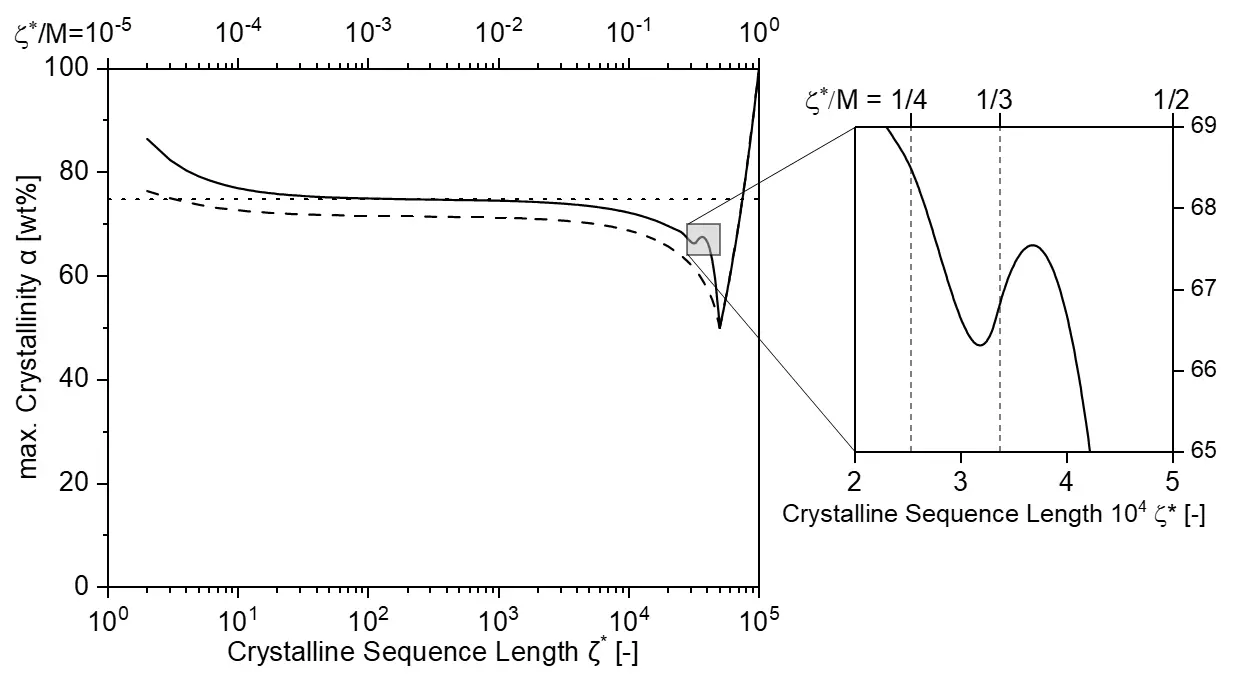
Figure 8. Maximal crystallinity as a function of $${\zeta }^{*}$$ for a polymer chain consisting of $$M=1\times {10}^{5}$$ segments by continuous treatment (Equation (19), solid line). The dashed line depicts the purely statistical treatment for the sake of comparability. Renyi’s constant (Equation (6)) is shown by the dotted line. A magnification is shown on the right side.
Figure 9 shows the prediction of the crystallinity of linear polyethylene as a function of the segment number for five different temperatures for both the statistical and the continuous treatment. For low molecular weights, both curves are identical and run down from fully crystalline to $$50\%$$. In this interval, only one crystalline sequence exists, and the crystallinity is predefined by the length of this sequence. After that, the crystallinity of the statistical treatment increases again due to the accommodation of more crystalline sequences in the polymer chain, levelling off at a crystallinity of about $$\alpha =72\%$$.
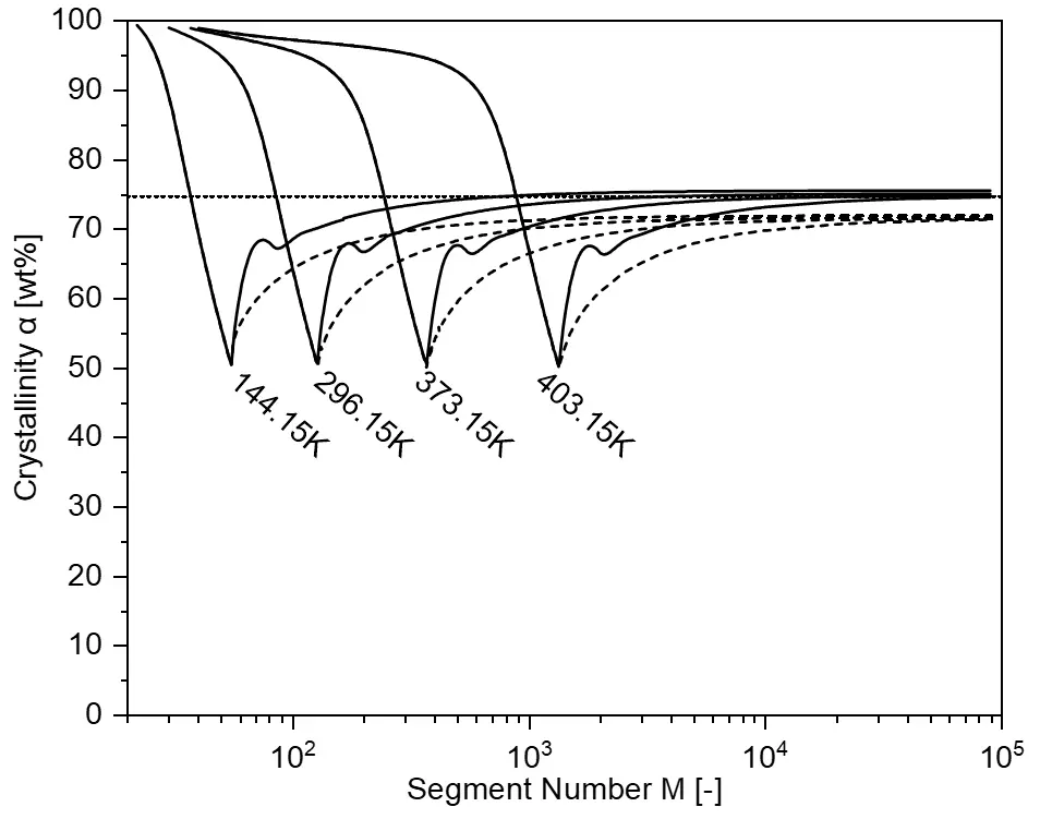
Figure 9. Prediction of the crystallinity of linear polyethylene as a function of the segment number $$M$$ for different temperatures indicated in the figure. The continuous treatment results in the solid line, while the statistical approach leads to the dashed line. The dotted line indicates Renyi’s constant (Equation (6)).
After the minimum in Figure 9, the curve for the continuous treatment increases as well, but at a higher level, and shows the local maximum already discussed in Figure 8. Subsequently, the continuous curve seems to run to an asymptotic limit close to Renyi’s constant. However, the curve does not converge and exceeds Renyi’s constant in case of low temperatures (hence short crystalline sequences) already in the range of reasonable change length. This exceeding of Renyi’s constant for low crystalline sequence length became already apparent in Figure 8. The Renyis constant is obtained for intermediate length of crystalline segments, while the length of the chain is long enough. For short crystalline sequences, a higher value of crystallinity can be obtained, which is physically absolutely reasonable. Consider a crystalline sequence of one. Here, a packing value of one (completely crystallized) would be possible.
Figure 10 shows the crystallinity as a function of temperature for different segment numbers. The crystallinity is decreasing with increasing temperature, since crystalline sequences become longer with increasing temperature, hence more wasted space is produced (Figure 6). For very high temperatures, the crystalline sequence is in the order of magnitude of the chain length, and theoretically, very high crystallinities can be obtained by a single very long crystalline sequence. For this to happen, the polymer chain must be defect-free, e.g., free of branches, knots, etc., which is unlikely to occur.
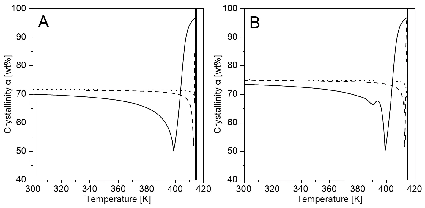
Figure 10. Prediction of the crystallinity of linear polyethylene as a function of the temperature for different segment numbers $$M$$ with statistical treatment (A) and continuous treatment (B). The solid lines denote $$M=1\times {10}^{3}$$, the dashed lines $$M=1\times {10}^{4}$$ and the dotted lines $$M=1\times {10}^{5}$$. The vertical bold line on the right denotes the melting temperature of linear polyethylene ($$414.6 \,\mathrm{K}$$ [56]).
3.2. Branched Polyethylene
3.2.1. Experimental Data
Figure 11 provides a comprehensive overview of existing experimental data [9,26,27,28,29,30,31,32,33,34,35,36,37,38,39,40,41,42,43,44,45,46,47,48] on the crystallinity of branched polyethylene measured by differential scanning calorimetry. Experimental data involving other experimental methods were excluded due to questionable assumptions when determining the crystallinity, and to keep the observations comparable.
The experimental data in Figure 11 underlie a clear trend where the maximal crystallinity of unbranched polyethylene lies around 60–75% while completely amorphous polyethylene exists in the region of around 100–150 branches per 1000 C-atoms. The measurements may be divided into two groups: Slowly cooled samples having cooling rates below $$20 \,\mathrm{K}/\mathrm{m}\mathrm{i}\mathrm{n}$$ and cooling in oil baths, as well as quenched samples having maximal possible cooling rates. Moreover, the target cooling temperature of the samples and the heating rate of the DSC measurement are issues. Furthermore, the amount and length of branching, as well as the molar mass distribution, polymerization method, and additives, must be considered. Since information on the above-mentioned influencing variables is often lacking and, in addition, all the variables are interrelated, it is challenging to extract clear dependencies from Figure 11.
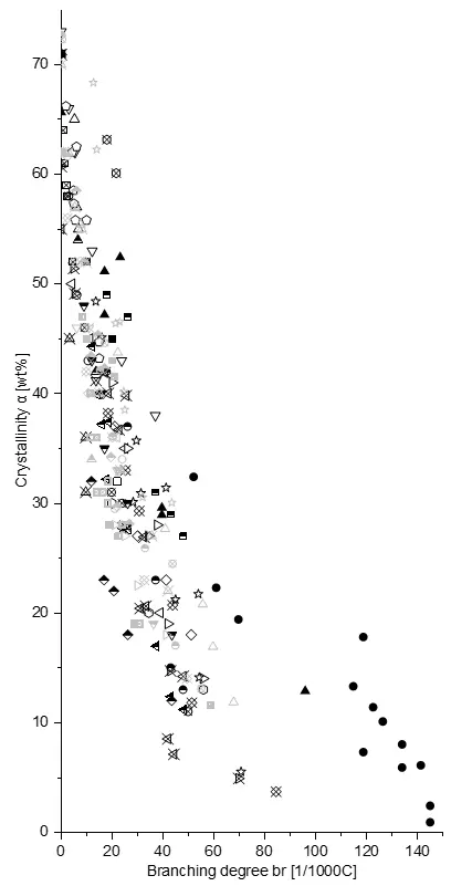
Figure 11. Experimental data concerning the crystallinity of polyethylene as a function of the branching degree br for slowly cooled (black) and quenched (grey) samples. References for experimental data are as follows:  : [30],
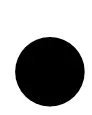 : [31],
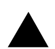 : [32],
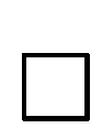 : [30],
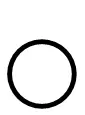 : [33],
 : [9],
 : [34],
 : [35],
 : [35],
 : [36],
 : [37],
 : [29],
 : [38],
 : [39],
 : [36],
 : [37],
 : [29],
 : [40],
 : [41],
 : [42],
 : [26],
 : [48],
 : [48],
 : [35],
 : [36],
 : [37],
 : [29],
 : [43],
 : [44],
 : [30],
 : [27],
 : [33],
 : [33],
 : [33],
 : [35],
 : [45],
 : [28],
 : [27],
 : [44],
 : [27],
 : [46],
 : [45],
 : [47],
 : [44],
 : [27],
 : [45],
 : [47],
 : [28],
 : [47]. More information such as the target temperature, the used heating rate, the length of the branching and the molecular weight are provided in Table 2.
Table 2. Information of the data in Figure 11. For slowly cooled samples, the first temperature indicates the target temperature (RT denotes room temperature) while the second one (dT) is the cooling rate (OB denotes oil bath). For quenched samples, just the target temperature is given. nbr represents the length of the branch, where C1 is methyl, C2 is ethyl, etc. MN indicates the molecular weight with a polydispersity index given in brackets where available. nrw denotes a narrow distribution, while n/a means not available.
|
Ref. |
T [°C] |
dT [K/min] |
nbr |
MN [kg/mol] |
||
|---|---|---|---|---|---|---|
|
Slowly Cooled |
|
[30] |
n/a |
n/a |
C1 |
200 (n/a) |
|
[31] |
RT |
10 |
C1 |
250 (n/a) |
|
|
[32] |
40 |
5 |
C1 |
n/a (n/a) |
|
|
[30] |
n/a |
n/a |
C2 |
100 (1.32) |
|
|
[33] |
n/a |
n/a |
C2 |
200 (12) |
|
|
[9] |
−50 |
10 |
C2 |
500 (2.3) |
|
|
[34] |
n/a |
15 |
C2 |
150 (6) |
|
|
[35] |
RT |
OB |
C2 |
100 (nrw) |
|
|
[35] |
RT |
OB |
C2 |
100 (nrw) |
|
|
[36] |
10 |
10 |
C2 |
100 |
|
|
[37] |
0 |
20 |
C2 |
100 |
|
|
[29] |
20 |
10 |
C2 |
n/a (n/a) |
|
|
[38] |
25 |
15 |
C2 |
8–30 (4–10) |
|
|
[39] |
n/a |
n/a |
C4 |
150 (13) |
|
|
[36] |
10 |
10 |
C4 |
100 (n/a) |
|
|
[37] |
0 |
20 |
C4 |
100 (n/a) |
|
|
[29] |
20 |
10 |
C4 |
n/a (n/a) |
|
|
[40] |
30 |
4.8 |
C4 |
100 (2.2) |
|
|
[41] |
40 |
10 |
C4 |
n/a (2–3) |
|
|
[42] |
50 |
2 |
C4 |
10–40 (n/a) |
|
|
[26] |
40 |
n/a |
C4 |
n/a (n/a) |
|
|
[48] |
−40 |
10 |
C6 |
n/a (n/a) |
|
|
[48] |
20 |
10 |
C6 |
n/a (n/a) |
|
|
[35] |
RT |
OB |
C6 |
100 (nrw) |
|
|
[36] |
0 |
10 |
C6 |
100 (n/a) |
|
|
[37] |
0 |
20 |
C6 |
100 (n/a) |
|
|
[29] |
20 |
10 |
C6 |
n/a (n/a) |
|
|
Quenched |
|
[43] |
−130 |
C1 |
200 (n/a) |
|
|
[44] |
35 |
C2 |
100 (2) |
||
|
[30] |
−130 |
C2 |
108 (1.32) |
||
|
[27] |
−20 |
C2 |
n/a (n/a) |
||
|
[33] |
−78 |
C2 |
125 (5) |
||
|
[33] |
40 |
C2 |
206 (5) |
||
|
[33] |
95 |
C2 |
108 (1.31) |
||
|
[35] |
−78 |
C2 |
100 (nrw) |
||
|
[45] |
0 |
C2 |
n/a (n/a) |
||
|
[28] |
0 |
C2 |
n/a (n/a) |
||
|
[27] |
−20 |
C3 |
n/a |
||
|
[44] |
−35 |
C4 |
100 (2) |
||
|
[27] |
−20 |
C4 |
n/a (n/a) |
||
|
[46] |
−150 |
C4 |
150 (n/a) |
||
|
[45] |
0 |
C4 |
n/a (n/a) |
||
|
[47] |
n/a |
C4 |
100 (2) |
||
|
[44] |
−35 |
C6 |
0.83 (2) |
||
|
[27] |
−20 |
C6 |
n/a (n/a) |
||
|
[45] |
0 |
C6 |
n/a (n/a) |
||
|
[47] |
n/a |
C6 |
100 (2) |
||
|
[28] |
0 |
C6 |
20–70 (5) |
||
|
[47] |
n/a |
C10 |
100 (2) |
No significant trend can be observed in Figure 11 regarding the type of cooling, although the target temperature of the quenched samples is mostly lower, which makes a comparison challenging. It appears that the crystallinity decreases as the branch length increases, when comparing different samples [27,28,29,36,37,45] with ethyl-, butyl-, and hexyl branched polyethylene at the same crystallization conditions. At the same time, Voigt-Martin et al. [35] measured no significant difference between ethyl- and hexyl-branched samples. Methyl-branches can be accommodated in the crystalline lattice up to a certain extent [58,65,66,67,68], which may explain why these systems [30,31,32] (filled symbols in Figure 11) exhibit a slightly higher crystallinity than the general trend. The influence of long-chain branches on the crystallinity is of minor importance, since their number is relatively small [69]. LDPE, for example, usually has approximately 20–25 short-chain branching points per 1000 carbon atoms and 0.5–1 long-chain branching points per 1000 carbon atoms, HDPE and LLDPE even less [69]. Moreover, due to their length, they can be incorporated in the crystal domains. The branching affects the crystallization behavior of the main chain, which is modeled by the Flory copolymer approach. As long as the main chain has long enough intervals to accommodate a crystalline length, crystallization occurs.
The same superposition of influences is evident when examining the effect of the target temperature on crystallinity in Figure 11. There seems to be a trend of higher crystallinities at lower temperatures when considering experimental data having similar conditions. Androsch and Wunderlich [48] measured the crystallinity of two hexyl-branched samples at −40 °C and 20 °C, exhibiting a significantly higher crystallinity for the lower temperature. Also, methyl-branched samples from Han-Adebekun et al. [32] at 40 °C have a significantly lower crystallinity than methyl-branched measurements from Ver Strate and Wilchinsky [31] at room temperature. On the other hand, quenched samples in Figure 11 show no large scatter across the crystallinity, although the range of target temperature (−130 °C to 95 °C) is much higher than for the slowly cooled systems (−50 °C to 30 °C).
3.2.2. Modelling Results
Model calculations were carried out in the following way: Via Equation (4) a crystalline sequence length $${\zeta }^{*}$$ for the linear polyethylene was calculated. Subsequently, with the help of $${\zeta }^{*}$$ and the CPP (Equation (1) or (19) respectively), a maximal crystallinity, $${\alpha }^{lin}$$, was calculated. Afterward, the crystallinity, $${\alpha }^{br}$$, is calculated using Equation (22). Finaly, the crystallinity, α, is obtained by multiplying both quantities.
Figure 12 shows the influence of several variables on the predicted crystallinity, namely the counting method of the CPP, the target temperature, the branching length as well as the molecular weight. Unless the indicated variables were varied, continuous treatment was chosen, the target temperature was set to $$T=273.15 \,\mathrm{K}$$ and polyethylene has butyl branches $$(n_\mathrm{br} = 4)$$ and a molecular weight of $${\mathrm{M}}_{\mathrm{N}}=100\,\mathrm{k}\mathrm{g}/\mathrm{m}\mathrm{o}\mathrm{l}$$ with parameters given in Table 1.
The predictive model correctly reproduces the general trend of experimental data in Figure 12. In particular, the limiting crystallinity of unbranched polyethylene, as determined by the CPP, is predicted accurately to be between 70% and 75%. Furthermore, Figure 12A shows the dependence on the treatment of the CPP. Choosing the continuous treatment results in a higher limiting crystallinity for unbranched polyethylene compared to the statistical treatment. This effect was already observed in Figure 9. The choice of treatment for the calculation of crystallinities is far from trivial, as it is a choice of mathematical abstraction for a complex, multivariate physical behavior. When considering a crystallization process, it seems obvious that sequences do not crystallize at exactly the same time. Even when considering quenched samples, there is probably a (very short) time lag between sequence crystallization due to inhibited motion or temperature gradients in the polymer. In view of that, the continuous treatment seems to be the more accurate abstraction. Moreover, the continuous treatment results in the classic Renyi constant for intermediate lengths of the crystalline sequences (Figure 8 and Figure 9). Henceforth, the continuous treatment is used for all subsequent calculations.
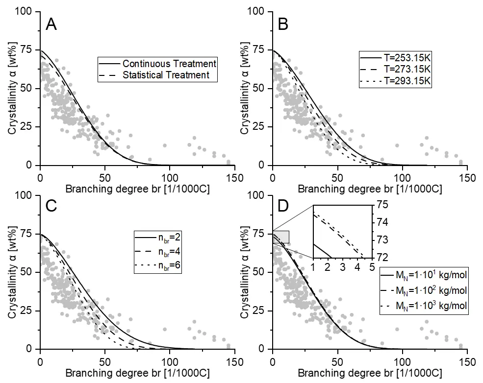
Figure 12. Model predictions for the crystallinity of polyethylene and its dependence on variables with parameters given in Table 1. Unless otherwise indicated, conditions were: $$T=273.15\mathrm{ }\,\mathrm{K},\mathrm{ }{M}_{N}=100\mathrm{ }\,\mathrm{k}\mathrm{g}/\mathrm{m}\mathrm{o}\mathrm{l},{n}_{br}=4$$, Continuous Treatment. (A): Dependence on the counting method for the CPP, (B): Dependence on the target temperature of crystallization, (C): Dependence on the length of branching (ethyl, butyl, and hexyl branches), (D): Dependence on molecular weight. Grey circles represent the experimental data from Figure 11.
The target temperature, whose influence on crystallinity is shown in Figure 12B, enters the model as a variable in calculating $${\zeta }^{*}$$ in Equation (4). However, its main influence is through the incorporation of the FCA in Equation (22). This results in higher crystallinities for lower temperatures in Figure 12B, which reproduces the observation that was found in Figure 11. According to Flory [5], at lower temperatures, shorter crystallites can exist in equilibrium. Hence, a rather short sequence that is enclosed between two branches must stay amorphous at higher temperatures but may crystallize at lower temperatures once this sequence is stable as a crystallite.
The length of the branching, $${n}_{br}$$, affects obviously only Equation (22), where branching is incorporated into the model. According to Figure 12C, longer branches result in a lower crystallinity, which agrees with experimental observations from Figure 11. The influence of the molecular weight of polyethylene on the crystallinity, which is shown in Figure 12D, affects just the crystallinity of the linear polyethylene. There is a slightly higher crystallinity for longer polyethylene chains. The exact limiting crystallinity can be discerned in Figure 9 and Figure 10.
In the next section, model predictions are compared with parts of the experimental data [29,36,48,49,50,56] from Figure 11. Since crystallinity depends on a variety of input variables, which have already been discussed, only measurements where sufficient input variables are available (at least target temperature, molecular weight, and branch length) will be considered.
Figure 13 shows the crystallinity of slowly cooled ethyl- and hexyl-branched polyethylene samples at $$T = 293.15 \,\mathrm{K}$$ and $${M}_{N} = 78\, \mathrm{k}\mathrm{g}\mathrm{m}\mathrm{o}{\mathrm{l}}^{-1}$$ from [29]. The effect of lower crystallinity as the branching length increases is clearly visible. The model predicts the experimental data in very high agreement, although there is a slight overestimation in the area of lower branching. The authors [29] performed measurements of samples polymerized with different catalysts. In Figure 13, just experimental data with metallocene catalyst are included due to their narrow branching distribution. Samples with a Ziegler-Natta type of catalyst were excluded due to their broad branching distribution [29]. There are different reasons for these slight overestimations, for instance, chain entanglements or kinetic issues. The incorporation of both effects leads to much more complexity, where the chain entanglements is discussed in the literature [6,9,10,11,12,13,14] in great detail. In order to take kinetic effects such as the cooling rate into account, an additional kinetic approach would be necessary, as only the equilibrium state can be described with the current theory.
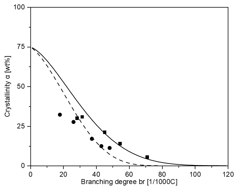
Figure 13. Predicted crystallinity of two slowly cooled sets of polyethylene samples, each having ethyl (squares, solid line) and hexyl (circles, dashed line) branches with target temperature $$T = 293.15 \,\mathrm{K}$$ and $${M}_{N}\approx 78\,\mathrm{k}\mathrm{g}/\mathrm{m}\mathrm{o}\mathrm{l}$$, parameters are given in Table 1. Experimental data taken from [29].
Figure 14 depicts the impact of the target temperature on a set of hexyl-branched polyethylene samples having a molecular weight of $${M}_{N}\approx 78\,\mathrm{k}\mathrm{g}/\mathrm{m}\mathrm{o}\mathrm{l}$$ with a molar mass distribution of $${\mathrm{M}}_{\mathrm{w}}/{\mathrm{M}}_{\mathrm{n}}\approx 2.35$$ [48]. The target temperatures were $$T=233.15\, \mathrm{K}$$ and $$T=293.15\, \mathrm{K}$$ respectively. As the temperature increases, the crystallinity decreases, which is in very good agreement with the model predictions.
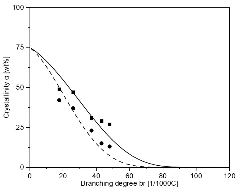
Figure 14. Predicted crystallinity of two slowly cooled sets of hexyl-branched polyethylene samples having temperatures of $$T=233.15 \,\mathrm{K}$$ (solid line, squares [48]) and $$T=293.15\, \mathrm{K}$$ (dashed line, circles [48]). No molecular weight is specified in the paper [48], so $${M}_{N}=100 \,\mathrm{k}\mathrm{g}\mathrm{m}\mathrm{o}{\mathrm{l}}^{-1}$$ is assumed, while the other parameters are given in Table 1.
To investigate the temperature dependence of crystallinity in more detail, Figure 15 shows the crystallinity for fixed branching degrees as a function of temperature. In general, the crystallinity decreases with increasing temperature, which can also be seen in Figure 12B. In Figure 15A, measurements from Starck et al. [36] show a decreasing crystallinity with increasing branch length, although the heavily branched sample ($$43.6\,\mathrm{ }\mathrm{b}\mathrm{r}\,\mathrm{ }1000{\mathrm{C}}^{-1}$$) has a higher crystallinity compared to measurements from Androsch and Wunderlich [49], having a similar branching degree ($$43\mathrm{ }\,\mathrm{b}\mathrm{r}\mathrm{ }\,1000{\mathrm{C}}^{-1}$$). The model correctly predicts the sigmoidal course of the temperature dependence. The combined CPP/FCA predicts the slightly branched samples from Starck et al. [36] in high agreement. However, the prediction of the heavily branched sample is in higher agreement with the measurement from Androsch and Wunderlich [49] than with the data from Starck et al. [36]. Both papers [36,49] use the heating run to measure the crystallinity at the same heating rate ($$10\mathrm{ }\,{\mathrm{K}\mathrm{m}\mathrm{i}\mathrm{n}}^{-1}$$) and use polymers having molecular weights between $${M}_{N}=50\,\mathrm{ }\mathrm{k}\mathrm{g}\mathrm{m}\mathrm{o}{\mathrm{l}}^{-1}$$ and $${M}_{N}=80\,\mathrm{ }\mathrm{k}\mathrm{g}\mathrm{m}\mathrm{o}{\mathrm{l}}^{-1}$$, such that the influence of the molecular weight on the crystallinity should be negligible (Figure 12D). The discrepancy between both experimental data sets [36,49] is pronounced at lower temperatures and almost vanishes in the range of the melting temperature. Possible reasons for the discrepancy could be differences in the production of the sample: Kim et al. [50] polymerized the samples in the laboratory with a metallocene catalyst, which results in a narrow branching distribution [65]. Androsch and Wunderlich [49] used a commercial polyethylene sample with an unknown polymerization procedure. Moreover, additives may also influence the crystallinity.
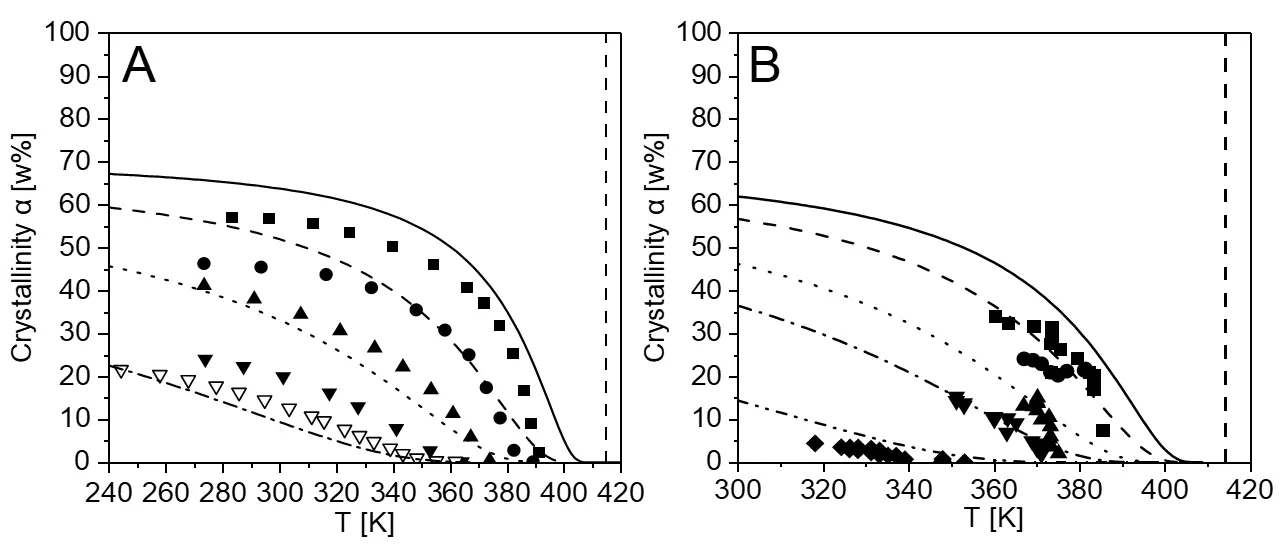
Figure 15. Temperature dependence of the crystallinity of hexyl-branched polyethylene having different branching degrees. (A): Filled symbols [36] having approx. $${M}_{W}=70\, \mathrm{k}\mathrm{g}\mathrm{m}\mathrm{o}{\mathrm{l}}^{-1}$$ and $$9\mathrm{ }\,\mathrm{b}\mathrm{r}1000{\mathrm{C}}^{-1}$$ (squares), $$15.8\, \mathrm{b}\mathrm{r}1000{\mathrm{C}}^{-1}$$ (circles), $$26 \,\mathrm{b}\mathrm{r}1000{\mathrm{C}}^{-1}$$ (triangles up) and $$43.6\,\mathrm{ }\mathrm{b}\mathrm{r}1000{\mathrm{C}}^{-1}$$ (triangles down). Open symbols [49] having $${M}_{N}=78\, \mathrm{k}\mathrm{g}\mathrm{m}\mathrm{o}{\mathrm{l}}^{-1}$$ and $$43\,\mathrm{ }\mathrm{b}\mathrm{r}1000{\mathrm{C}}^{-1}$$. (B): Experimental data [50], having approx. $${M}_{N}=23\, \mathrm{k}\mathrm{g}\mathrm{m}\mathrm{o}{\mathrm{l}}^{-1}$$ and $$9.9\,\mathrm{ }\mathrm{b}\mathrm{r}1000{\mathrm{C}}^{-1}$$ (squares), $$12.9\, \mathrm{b}\mathrm{r}1000{\mathrm{C}}^{-1}$$ (circles), $$18.2\,\mathrm{ }\mathrm{b}\mathrm{r}1000{\mathrm{C}}^{-1}$$ (triangles up), $$24.0\,\mathrm{ }\mathrm{b}\mathrm{r}1000{\mathrm{C}}^{-1}$$ (triangles down) and $$38.6\,\mathrm{ }\mathrm{b}\mathrm{r}1000{\mathrm{C}}^{-1}$$ (diamonds). Lines in A and B are predictions with the combined CPP/FCA with parameters given in Table 1. The vertical dashed lines denote the melting temperature of linear polyethylene ($$414.6\, \mathrm{K}$$ [56]).
The predicted melting point depression in Figure 15A, i.e., the decrease in melting point due to the inclusion of branches in the highly branched samples, is in very good agreement with both experimental data sets [36,49]. However, the melting point depressions of the slightly branched samples are smaller than those in the experiment [36]. Figure 15B compares the predicted influence of the temperature on the crystallinity with experimental data from Kim et al. [50], which is in very high agreement. Especially the high and medium branched samples are reproduced very well, while the little branched sample is slightly overestimated.
4. Conclusions
In this work, a theory for predicting the crystallinity of branched polyethylene was derived. Starting at the crystallinity of linear polyethylene, the car-parking-problem was incorporated and applied by statistical and continuous treatment, by which the influence of the molecular weight on linear polyethylene could be studied. Furthermore, the influence of the polyethylene architecture on the crystallinity was investigated by incorporating branches along the backbone. The influence of several variables was compared with experimental data and revealed exceptional results. Slight overestimations of the crystallinity in the area of lower branching degrees may be attributed to chain entanglement.
Author Contributions
Conceptualization, S.L., M.F. and S.E.; Methodology, S.L., M.F. and S.E.; Software, S.L.; Validation, S.L., M.F. and S.E.; Formal Analysis, S.L.; Investigation, S.L., M.F. and S.E.; Writing—Original Draft Preparation, S.L.; Writing—Review & Editing, S.L., M.F. and S.E.; Visualization, S.L.; Supervision, M.F. and S.E.
Ethics Statement
Not applicable.
Informed Consent Statement
Not applicable.
Data Availability Statement
The original data are available on request via e-mail.
Funding
This research received no external funding.
Declaration of Competing Interest
There are no financial interests. There are no financial and personal relationships with other people or organizations that could inappropriately influence (bias) their work.
References
- Müller AJ, Arnal ML. Thermal fractionation of polymers. Prog. Polym. Sci. 2005, 30, 559–603. DOI:10.1016/j.progpolymsci.2005.03.001 [Google Scholar]
-
Mandelkern L. Crystallization of Polymers: Equilibrium Concepts, 2nd ed.; Cambridge University Press: Cambridge, UK, 2002. [Google Scholar]
-
He FA, Zhang LM. Study on branching structure, melting, and crystallization of polyethylene prepared by nickel α-diimine catalyst covalently intercalated inside OapPOSS-modified laponite clay gallery. Polym. Test. 2014, 35, 80–86. DOI:10.1016/j.polymertesting.2014.03.001 [Google Scholar]
-
Fischlschweiger M, Enders S. Solid–liquid equilibria of crystalline and semi-crystalline monodisperse polymers, taking into account the molecular architecture by application of the lattice cluster theory. Mol. Phys. 2014, 112, 3109–3119. DOI:10.1080/00268976.2014.931605 [Google Scholar]
-
Flory PJ. Theory of crystallization in copolymers. Trans. Farad. Soc. 1955, 51, 848–857. DOI:10.1039/TF9555100848 [Google Scholar]
-
Flory PJ, Yoon DY. Molecular morphology in semicrystalline polymers. Nature 1978, 272, 226–229. DOI:10.1038/272226a0 [Google Scholar]
-
Mandelkern L, Allou AL, Gopalan MR. Enthalpy of fusion of linear polyethylene. J. Phys. Chem. 1968, 72, 309–318. DOI:10.1021/j100847a060 [Google Scholar]
-
Mandelkern L. Crystallization of Polymers: Kinetics and Mechanisms, 2nd ed.; Cambridge University Press: Cambridge, UK, 2009. DOI:10.1017/CBO9780511535413 [Google Scholar]
-
Moyassari A, Mostafavi H, Gkourmpis T, Hedenqvist MS, Gedde UW, Nilsson F. Simulation of semi-crystalline polyethylene: Effect of short-chain branching on tie chains and trapped entanglements. Polymer 2015, 72, 177–184. DOI:10.1016/j.polymer.2015.07.008 [Google Scholar]
-
Psarski M, Piorkowska E, Galeski A. Crystallization of Polyethylene from Melt with Lowered Chain Entanglements. Macromolecules 2000, 33, 916–932. DOI:10.1021/ma990298h [Google Scholar]
-
Yamazaki S, Hikosaka M, Toda A, Wataoka I, Gu F. Role of entanglement in nucleation and melt relaxation of polyethylene. Polymer 2002, 43, 6585–6593. DOI:10.1016/S0032-3861(02)00592-X [Google Scholar]
-
Bu H, Gu F, Bao L, Chen M. Influence of Entanglements on Crystallization of Macromolecules. Macromolecules 1998, 31, 7108–7110. DOI:10.1021/ma980713q [Google Scholar]
-
Iwata K. Role of entanglement in crystalline polymers 1. Basic theory. Polymer 2002, 43, 6609–6626. DOI:10.1016/S0032-3861(02)00524-4 [Google Scholar]
-
Nilsson F, Lan X, Gkourmpis T, Hedenqvist MS, Gedde UW. Modelling tie chains and trapped entanglements in polyethylene. Polymer 2012, 53, 3594–3601. DOI:10.1016/j.polymer.2012.05.045 [Google Scholar]
-
Stribeck N. Oriented Quiescent Crystallization of Polyethylene Studied by USAXS. Macromol. Chem. Phys. 2004, 205, 1455–1462. DOI:10.1002/macp.200400035 [Google Scholar]
-
Gornick F, Jackson JL. Sequence Selection Problem in the Crystallization of Polymers. J. Chem. Phys. 1963, 38, 1150–1154. DOI:10.1063/1.1733816 [Google Scholar]
-
Maltz A, Mola EE. Average saturation coverage for one-dimensional arrays of β-bell particles. Surf. Sci. 1982, 115, 599–605. DOI:10.1016/0039-6028(82)90390-9 [Google Scholar]
-
Gordon M, Hillier IH. Statistics of Random Placement, Subject to Restrictions, on a Linear Lattice. J. Chem. Phys. 1963, 38, 1376–1380. DOI:10.1063/1.1733861 [Google Scholar]
-
Renyi A. On a One-Dimensional Problem Concerning Random Space-Filling; Mathematical Institute of the Hungarian Academy of Sciences: Budapest, Hungary, 1958; Volume 3, pp. 109–127. [Google Scholar]
-
Evans JW. Random and cooperative sequential adsorption. Rev. Modern Phys. 1993, 65, 1281–1329. DOI:10.1103/RevModPhys.65.1281 [Google Scholar]
-
Bonnier B, Boyer D, Viot P. Pair correlation function in random sequential adsorption processes. J. Phys. A Math. Gen. 1994, 27, 3671–3682. DOI:10.1088/0305-4470/27/11/017 [Google Scholar]
-
McQuistan RB, Lichtman D. Exact Occupation Kinetics for One–Dimensional Arrays of Dumbbells. J. Math. Phys. 1968, 9, 1680–1684. DOI:10.1063/1.1664497 [Google Scholar]
-
McQuistan RB, Lichtman D, Levine LP. Adsorption statistics for immobile, diatomic molecules. Surf. Sci. 1970, 20, 401–410. DOI:10.1016/0039-6028(70)90190-1 [Google Scholar]
-
Maltz A, Mola EE. Continuous one–dimensional average unsaturated coverage as the limit of a lattice model. J. Chem. Phys. 1983, 79, 5141–5144. DOI:10.1063/1.445639 [Google Scholar]
-
Gornick F, Freedman RW. Reactions of adjacent substituents on polymer chains: Combinatorial consequences of the mechanism. J. Math. Chem. 1990, 5, 265–274. DOI:10.1007/BF01166357 [Google Scholar]
-
Novak A, Bobak M, Kosek J, Banaszak BJ, Lo D, Widya T, et al. Ethylene and 1-hexene sorption in LLDPE under typical gas-phase reactor conditions: Experiments. J. Appl. Polym. Sci. 2006, 100, 1124–1136. DOI:10.1002/app.23508 [Google Scholar]
-
Alizadeh A, Richardson L, Xu J, McCartney S, Marand H, Cheung YW, et al. Influence of Structural and Topological Constraints on the Crystallization and Melting Behavior of Polymers. 1. Ethylene/1-Octene Copolymers. Macromolecules 1999, 32, 6221–6235. DOI:10.1021/ma990669u [Google Scholar]
-
Hay JN, Zhou XQ. Incorporation of branches into the crystal lattice during the solidification of linear low density polyethylene. Polymer 1993, 34, 1002–1005. DOI:10.1016/0032-3861(93)90221-U [Google Scholar]
-
Keating MY, Lee IH. Glass transition, crystallinity, resin stiffness, and branch distribution in metallocene and Ziegler-Natta ethylene 1-olefins. J. Macromol. Sci. Part B 1999, 38, 379–401. DOI:10.1080/00222349908212439 [Google Scholar]
-
Axelson DE, Mandelkern L, Popli R, Mathieu P. Carbon-13 NMR of polyethylenes: Correlation of the crystalline component T1 with structure. J. Polym. Sci. Polym. Phys. Ed. 1983, 21, 2319–2335. DOI:10.1002/pol.1983.180211109 [Google Scholar]
-
Ver Strate G, Wilchinsky ZW. Ethylene-propylene copolymers: Degree of crystallinity and composition. J. Polym. Sci. Part A-2 Polym. Phys. 1971, 9, 127–142. DOI:10.1002/pol.1971.160090109 [Google Scholar]
-
Han-Adebekun GC, Hamba M, Ray WH. Kinetic study of gas phase olefin polymerization with a TiCl4/MgCl2 catalyst I. Effect of polymerization conditions. J. Polym. Sci. Part A Polym. Chem. 1997, 35, 2063–2074. DOI:10.1002/(SICI)1099-0518(19970730)35:10<2063::AID-POLA22>3.0.CO;2-D [Google Scholar]
-
Glotin M, Mandelkern L. A Raman spectroscopic study of the morphological structure of the polyethylenes. Coll. Polym. Sci. 1982, 260, 182–192. DOI:10.1007/BF01465438 [Google Scholar]
-
Seguela R, Rietsch F. Tensile drawing behaviour of ethylene/α-olefin copolymers: influence of the co-unit concentration. Polymer 1986, 27, 703–708. DOI:10.1016/0032-3861(86)90127-8 [Google Scholar]
-
Voigt‐Martin IG, Alamo RG, Mandelkern L. A quantitative electron microscopic study of the crystalline structure of ethylene copolymers. J. Polym. Sci. Part B Polym. Phys. 1986, 24, 1283–1302. DOI:10.1002/polb.1986.090240608 [Google Scholar]
-
Starck P, Rajanen K, Löfgren B. Comparative studies of ethylene–α-olefin copolymers by thermal fractionations and temperature-dependent crystallinity measurements. Thermochim. Acta 2003, 395, 169–181. DOI:10.1016/S0040-6031(02)00138-7 [Google Scholar]
-
Jokela K, Väänänen A, Torkkeli M, Starck P, Serimaa R, Löfgren B, et al. Differential scanning calorimetry, small-angle X-ray scattering, and wide-angle X-ray scattering on homogeneous and heterogeneous ethylene-α-copolymers. J. Polym. Sci. Part B Polym. Phys. 2001, 39, 1860–1875. DOI:10.1002/polb.1161 [Google Scholar]
-
Hedenqvist M, Angelstok A, Edsberg L, Larsson PT, Gedde UW. Diffusion of small-molecule penetrants in polyethylene: Free volume and morphology. Polymer 1996, 37, 2887–2902. DOI:10.1016/0032-3861(96)89384-0 [Google Scholar]
-
Huang Y-L, Brown N. Dependence of slow crack growth in polyethylene on butyl branch density: Morphology and theory. J. Polym. Sci. Part B Polym. Phys. 1991, 29, 129–137. DOI:10.1002/polb.1991.090290116 [Google Scholar]
-
Mirabella FM, Bafna A. Determination of the crystallinity of polyethylene/α-olefin copolymers by thermal analysis: Relationship of the heat of fusion of 100% polyethylene crystal and the density. J. Polym. Sci. Part B Polym. Phys. 2002, 40, 1637–1643. DOI:10.1002/polb.10228 [Google Scholar]
-
Quijada R, Rojas R, Mauler RS, Galland GB, Scipioni RB. Study of the effect of the monomer pressure on the copolymerization of ethylene with 1-hexene. J. Appl. Polym. Sci. 1997, 64, 2567–2574. DOI:10.1002/(SICI)1097-4628(19970627)64:13<2567::AID-APP10>3.0.CO;2-X [Google Scholar]
-
Chien JCW, Nozaki T. Ethylene–hexene copolymerization by heterogeneous and homogeneous Ziegler–Natta catalysts and the “comonomer” effect. J. Polym. Sci. Part A Polym. Chem. 1993, 31, 227–237. DOI:10.1002/pola.1993.080310127 [Google Scholar]
-
Axelson DE. Crystalline order in polyethylene: A 13C NMR CP/MAS solid-state T1 study. J. Polym. Sci. Polym. Phys. Ed. 1982, 20, 1427–1435. DOI:10.1002/pol.1982.180200808 [Google Scholar]
-
Alamo RG, Mandelkern L. Thermodynamic and structural properties of ethylene copolymers. Macromolecules 1989, 22, 1273–1277. DOI:10.1021/MA00193A045 [Google Scholar]
-
France C, Hendra PJ, Maddams WF, Willis HA. A study of linear low-density polyethylenes: Branch content, branch distribution and crystallinity. Polymer 1987, 28, 710–712. DOI:10.1016/0032-3861(87)90216-3 [Google Scholar]
-
Martín S, Expósito MT, Vega JF, Martínez‐Salazar J. Microstructure and properties of branched polyethylene: Application of a three-phase structural model. J. Appl. Polym. Sci. 2012, 128, 1871–1878. DOI:10.1002/app.38290 [Google Scholar]
-
Laguna MF, Cerrada ML, Benavente R, Pérez E, Quijada R. Permeation measurements in ethylene-1-hexene, ethylene-1-octene, and ethylene-1-dodecene copolymers synthesized with metallocene catalysts. J. Polym. Sci. Part B Polym. Phys. 2003, 41, 2174–2184. DOI:10.1002/polb.10577 [Google Scholar]
-
Androsch R, Wunderlich B. A Study of Annealing of Poly(ethylene-co-octene) by Temperature-Modulated and Standard Differential Scanning Calorimetry. Macromolecules 1999, 32, 7238–7247. DOI:10.1021/ma9905223 [Google Scholar]
-
Androsch R, Wunderlich B. Analysis of the Degree of Reversibility of Crystallization and Melting in Poly(ethylene-co-1-octene). Macromolecules 2000, 33, 9076–9089. DOI:10.1021/ma000504h [Google Scholar]
-
Kim M-H, Phillips PJ, Lin JS. The equilibrium melting points of random ethylene-octene copolymers: A test of the Flory and Sanchez-Eby theories. J. Polym. Sci. Part B Polym. Phys. 2000, 38, 154–170. DOI:10.1002/(SICI)1099-0488(20000101)38:1<154::AID-POLB19>3.0.CO;2-1 [Google Scholar]
-
Flory PJ. Thermodynamics of Crystallization in High Polymers. IV. A Theory of Crystalline States and Fusion in Polymers, Copolymers, and Their Mixtures with Diluents. J. Chem. Phys. 1949, 17, 223–240. DOI:10.1063/1.1747230 [Google Scholar]
-
Mandelkern L, Fatou JG, Howard C. The Nucleation of Long-Chain Molecules 1. J. Phys. Chem. 1964, 68, 3386–3391. DOI:10.1021/j100793a047 [Google Scholar]
-
Mandelkern L. Crystallization Kinetics in High Polymers. II. Polymer-Diluent Mixtures. J. Appl. Phys. 1955, 26, 443–451. DOI:10.1063/1.1722016 [Google Scholar]
-
Hoffman JD, Frolen LJ, Ross GS, Lauritzen JI. On the Growth Rate of Spherulites and Axialites from the Melt in Polyethylene Fractions: Regime I and Regime II Crystallization. J. Res. Nat. Bur. Stand. Sect. A Phys. Chem. 1975, 79A, 671–699. DOI:10.6028/jres.079a.026 [Google Scholar]
-
Quinn FA, Mandelkern L. Thermodynamics of Crystallization in High Polymers: Poly-(ethylene) 1. J. Am. Chem. Soc. 1958, 80, 3178–3182. DOI:10.1021/ja01546a003 [Google Scholar]
-
Wunderlich B, Czornyj G. A Study of Equilibrium Melting of Polyethylene. Macromolecules 1977, 10, 906–913. DOI:10.1021/ma60059a006 [Google Scholar]
-
Clark ES. Unit Cell Information on Some Important Polymers. In Physical Properties of Polymers Handbook, 2nd ed.; Mark JE, Ed.; Springer: New York, NY, USA, 2007. [Google Scholar]
-
Richardson MJ, Flory PJ, Jackson JB. Crystallization and melting of copolymers of polymethylene. Polymer 1963, 4, 221–236. DOI:10.1016/0032-3861(63)90028-4 [Google Scholar]
-
Freedman RW, Gornick F. Further reflections on the one-dimensional packing problem. J. Math. Chem. 1993, 13, 167–176. DOI:10.1007/BF01165562 [Google Scholar]
-
Kilian HG. Partiell kristallisierende Copolymere als pseudoeutektische Systeme. Coll. Polym. Sci. 1965, 202, 97–107. DOI:10.1007/BF01497096 [Google Scholar]
-
Baur H. Zur Theorie der Kristallisation in Copolymeren. Coll. Polym. Sci. 1965, 203, 97–107. DOI:10.1007/BF01507753 [Google Scholar]
-
Wunderlich B. Macromolecular Physics: Crystal Nucleation, Growth, Annealing; Academic Press: New York, NY, USA, 1976. [Google Scholar]
-
Mandelkern L. The effect of molecular weight on the crystallization, melting, and morphology of long-chain molecules. J. Polym. Sci. Part C Polym. Symp. 1967, 15, 129–162. DOI:10.1002/polc.5070150112 [Google Scholar]
-
Anderson FR. Morphology of Isothermally Bulk–Crystallized Linear Polyethylene. J. Appl. Phys. 1964, 35, 64–70. DOI:10.1063/1.1713100 [Google Scholar]
-
Alamo RG, Mandelkern L. The crystallization behavior of random copolymers of ethylene. Thermochim. Acta 1994, 238, 155–201. DOI:10.1016/S0040-6031(94)85210-3 [Google Scholar]
-
Martuscelli E, Pracella M. Effects of chain defects on the thermal behaviour of polyethylene. Polymer 1974, 15, 306–314. DOI:10.1016/0032-3861(74)90128-1 [Google Scholar]
-
Perez E, Vanderhart DL, Crist B, Howard PR. Morphological partitioning of ethyl branches in polyethylene by carbon-13 NMR. Macromolecules 1987, 20, 78–87. DOI:10.1021/ma00167a015 [Google Scholar]
-
Pérez E, Vanderhart DL. Morphological partitioning of chain ends and methyl branches in melt-crystallized polyethylene by 13C-NMR. J. Polym. Sci. Part B Polym. Phys. 1987, 25, 1637–1653. DOI:10.1002/polb.1987.090250807 [Google Scholar]
-
Kissin YV. “Catalysts for the Manufacture of Polyethylene”. In Handbook of Industrial Polyethylene and Technology; Spalding MA, Chatterjee AM, Eds.; Wiley: Hoboken, NJ, USA, 2017. [Google Scholar]