
Contrasting Wave Power Intensity and Resource Quality in the Northwest Pacific: Variability, Availability, and Extreme Load Risk
Contrasting Wave Power Intensity and Resource Quality in the Northwest Pacific: Variability, Availability, and Extreme Load Risk
Xincong Chen
1
 Zhimeng Zhang
1,2,*
Chunning Ji
1,3
Weilin Chen
1
Dong Xu
4
Zhimeng Zhang
1,2,*
Chunning Ji
1,3
Weilin Chen
1
Dong Xu
4
Received: 22 June 2026 Revised: 13 July 2026 Accepted: 28 July 2026 Published: 04 August 2026

© 2026 The authors. This is an open access article under the Creative Commons Attribution 4.0 International License (https://creativecommons.org/licenses/by/4.0/).
1. Introduction
Ocean wave energy is a promising marine renewable resource because surface waves can store and transport substantial mechanical energy over long distances, providing a potentially dense and complementary source of low-carbon power for coastal and island regions [1,2]. Over the past two decades, global and regional assessments have greatly advanced the understanding of where large wave-energy resources are located. Early global atlases and hindcast-based studies showed that the strongest theoretical wave-power resources are generally concentrated in the mid- to high-latitude oceans and along exposed western continental margins, where persistent winds and storm activity maintain large wave heights and long wave periods [3,4,5,6]. More recent studies have further shown that wave power is nonstationary, varying across seasonal, interannual, and climatic time scales, and may respond to large-scale ocean warming and changes in atmospheric circulation [7,8,9]. These studies provide the foundation for modern wave-energy resource assessment, but they also expose a limitation of a purely intensity-based view: large mean wave power does not necessarily imply a high-quality resource for practical exploitation.
This limitation has become increasingly important in wave-energy assessment practice. Technical guidelines and review studies emphasize that resource characterization should include not only mean wave-power magnitude but also temporal variability, persistence, uncertainty, and deployment-relevant constraints [10,11]. The International Electrotechnical Commission Technical Specification (IEC TS) 62600-101 framework, for example, defines procedures for estimating, analyzing, and reporting wave-energy resources at potential wave energy converter (WEC) sites, whereas guidance from the European Marine Energy Centre (EMEC) explicitly distinguishes short-term instantaneous wave power from the longer-term wave-power climate, including monthly, seasonal, annual, and interannual variability. These recommendations reflect a broader shift in the field: the relevant question is no longer simply where waves are energetic, but where wave-energy resources are energetic, persistent, predictable, and operationally manageable.
This shift has also led to divergent interpretations of wave-energy potential. A conventional view favors the most energetic regions because higher mean wave power can increase theoretical production and improve the energetic attractiveness of a site. However, another perspective argues that lower- or moderate-energy environments may be more feasible when lower variability, reduced survivability constraints, higher device availability, and more favorable capacity-factor behavior are considered [12,13,14]. This tension is central to wave-energy development. High-energy regions can provide large theoretical resources, but they may also impose stronger structural loads, greater downtime, and higher design costs. Moderate-energy regions may offer lower gross power but can become more attractive if the resource is more persistent and less exposed to extreme sea states. Therefore, wave-energy potential should be assessed by distinguishing resource intensity from resource quality [15].
This distinction is particularly important in storm-dominated basins. In such regions, high mean and high-percentile wave power are often generated by extratropical storms, monsoonal surges, or tropical cyclones. These forcing systems can produce high wave-power densities, but they can also create pronounced seasonality, intermittent resource windows, and elevated extreme-load exposure. From an engineering perspective, this creates an intensity–persistence–risk trade-off. A site with very high mean wave power may be less favorable if its energy is concentrated within short storm-driven periods or if it is frequently exposed to extreme wave events. Conversely, a site with moderate wave power may represent a higher-quality resource if it provides more continuous availability, lower temporal variability, and lower risk exposure. Although many regional assessments now include seasonal means or high-percentile statistics, the combined structure of wave-power intensity, persistence, and risk is still less commonly diagnosed as an integrated resource-quality problem.
A further underdeveloped dimension is the physical origin of the wave-energy resource. Ocean waves in a given region may be dominated by locally generated wind seas, remotely generated swells, or mixed sea states. These wave systems have different implications for resource quality. Wind-sea-dominated conditions are more directly connected to local winds and storm activity and therefore tend to be more energetic but also more variable and risk-prone. Swell-dominated conditions, by contrast, are associated with waves generated remotely and propagated over long distances; they often have longer periods and smoother temporal evolution, which may favor persistence and operational predictability. The distinction between wind sea and swell is well established in wave-climatology and spectral-partitioning studies [16,17,18], and global analyses have shown that swell dominates large parts of the open-ocean wave climate [16]. Nevertheless, wind-sea/swell composition has rarely been used as a central explanatory variable in wave-energy resource-quality assessment. This leaves an important question unresolved: is the mismatch between high wave-power intensity and high-quality wave-energy resources controlled, at least partly, by wave-system source composition?
The Northwest Pacific provides a suitable natural laboratory for addressing this question. The basin contains a wide range of wave-energy environments, including the northern South China Sea, East China Sea shelf, Philippine Sea, Ryukyu–Kuroshio transition zone, Kuroshio Extension region, and the mid- to high-latitude storm belt. These regions are influenced by different combinations of East Asian monsoon forcing, tropical cyclones, extratropical storms, western-boundary-current environments, remote swell propagation, and shelf–open-ocean contrasts. Previous studies have assessed wave-energy resources in China’s adjacent seas, including the East China Sea, South China Sea, and offshore China, using SWAN, WAVEWATCH III, satellite observations, buoy data, and reanalysis products [19,20,21,22,23,24]. These studies have shown strong spatial and seasonal differences among marginal seas and coastal waters and have provided important baseline knowledge for regional resource evaluation. However, most existing work has focused on resource magnitude, seasonal distribution, or site-level potential. The broader basin-scale question of how wave-energy intensity, persistence, risk exposure, and wind-sea/swell source structure interact across the Northwest Pacific remains insufficiently resolved.
Satellite altimetry provides broad spatial coverage and increasingly long time series, making it particularly valuable where long-term buoy observations are sparse. Multi-satellite altimeter data have been used to assess wave-energy resources in China’s seas [22], while recent studies have applied SWIM radar and high-resolution altimetry to wave-power assessments along European Atlantic coasts and in the Mediterranean Sea [25,26]. Satellite altimetry, therefore, provides an important observational complement to reanalysis and numerical hindcasts, although its intermittent temporal sampling and uncertainties in coastal retrievals and wave-period estimation should be considered.
Long-term reanalysis products make it possible to examine these relationships consistently at the basin scale. ERA5, the fifth-generation global reanalysis produced by the European Centre for Medium-Range Weather Forecasts (ECMWF), provides hourly global atmospheric and ocean-wave variables from 1979 onward, including significant wave height, wave periods, wind-wave height, swell height, wave direction, 10 m winds, mean sea-level pressure, bathymetry, and other wave diagnostics [27]. ERA5 has been widely used for climatological wave analysis and preliminary resource-scale assessment, and validation studies have generally shown useful skill for significant wave height and wave period under broad climatological conditions, while also noting limitations in shallow waters, tropical-cyclone conditions, and extremes [28,29,30,31]. In particular, severe ERA5 winds can be negatively biased, resulting in an underestimation of extreme wave conditions when significant wave height exceeds approximately 7.5 m [32]. ERA5 is therefore appropriate for basin-scale resource-quality diagnosis and technical pre-screening, provided that it is not overinterpreted as a substitute for high-resolution nearshore modeling, bias-corrected extreme-wave hindcasts, device-specific power matrices, or final site-level validation.
The Northwest Pacific features a complex wave climate governed by the East Asian monsoon, frequent tropical cyclones, extratropical storms, and extensive open-ocean fetch, producing pronounced spatial gradients in wave-energy characteristics. Rather than merely identifying zones of maximum energy, this study evaluates whether high-power regions also provide operationally favorable resources. The primary contribution is an integrated diagnosis of the spatial decoupling between theoretical wave-power intensity and practical resource quality: Section 3.1 characterizes resource intensity and sea-state structure; Section 3.2 evaluates temporal stability, availability, and persistence; Section 3.3 examines extreme-load and wave-amplification risk; Section 3.4 relates resource-quality contrasts to wind-sea/swell composition; and Section 3.5 integrates these dimensions into a technical pre-screening framework.
2. Materials and Methods
2.1. Study Area, Data Source, and Processing Framework
The study domain covers the Northwest Pacific (NWP) between 0–60° N and 100–180° E. This domain spans marginal seas, continental shelves, subtropical open-ocean regions, the Ryukyu–Kuroshio transition, the Kuroshio Extension, and the mid- to high-latitude storm belt. To reduce the masking effect of basin-scale averaging, six diagnostic subregions were defined for comparative analysis: the Northern South China Sea (NSCS; 10–22° N, 110–120° E), Philippine Sea (PS; 10–22° N, 125–145° E), East China Sea Shelf (ECSS; 24–32° N, 122–128° E), Ryukyu–Kuroshio Transition Zone (RKTZ; 24–32° N, 128–136° E), Kuroshio Extension Onset Region (KEOR; 30–38° N, 136–150° E), and Mid- to High-Latitude Storm Belt (MHSB; 38–50° N, 145–170° E). These subregions were not intended to represent fixed dynamical boundaries; rather, they provide a reproducible geographical framework for comparing low-latitude marginal-sea, shelf, western-boundary-current, open-ocean, and storm-belt wave-energy environments. The same domain and subregional boxes were implemented on a regular 0.5° longitude–latitude grid.
The analysis used 45 years of six-hourly ERA5 wave data covering 1979–2023. ERA5 is the fifth-generation ECMWF global reanalysis and provides hourly global atmospheric, land, and ocean-wave fields [27]. The variables extracted in this study were significant wave height of combined wind waves and swell, Hs; mean wave period, Tm; peak wave period, Tp; significant height of wind waves, Hs,wind; significant height of total swell, Hs,swell; maximum individual wave height, Hmax; and model bathymetry. These variables were used for wave-power estimation, wind-sea/swell source diagnosis, risk-proxy construction, and depth-constrained technical screening within a consistent multidecadal framework. Wave power, percentile thresholds, availability, variability, risk, and screening-score fields were subsequently derived from these variables. The effective temporal sampling rate was four records per day, corresponding to the six-hourly data interval. The 24 h declustering interval used in the event analysis, therefore, corresponded to four consecutive time steps.
ERA5 Hmax was used only as a relative risk proxy. ECMWF defines maximum individual wave height as a model-based estimate of the expected highest individual wave within a short time window rather than a direct observation of an individual wave [33]. Therefore, all Hmax-derived diagnostics in this study are interpreted as relative amplification-risk indicators, not as observed rogue-wave occurrence statistics.
2.2. Wave-Power Estimation and Wind-Sea/Swell Source Metrics
For deep-water waves, wave-power density per unit wave-crest width can be approximated as:
where J is expressed in kW·m−1, Hs is the significant wave height in metres, and Te is the energy period in seconds. This formulation is widely used in first-order wave-energy resource assessment because energy flux scales with both wave-height variance and characteristic period [3,4,5,6,7,10,11]. The energy period is generally preferred for wave-energy resource characterization because it is directly linked to spectral energy flux [12,13]. Because Te was not available in the processed ERA5 dataset, the standard ERA5 mean wave period, Tm, was used as a proxy. Since energy flux depends on Te, a spectral conversion factor is typically required when standard mean wave periods are used; for example, Te ≈ 1.14Tm for a Pierson–Moskowitz spectrum or Te ≈ 1.05Tm for a JONSWAP spectrum. For this basin-scale assessment, Jm(t) was calculated using the unadjusted mean-period proxy to provide a conservative baseline:
A peak-period-based estimate was calculated as a sensitivity case:
The Jm field was used as the principal wave-power variable throughout the analysis, whereas Jp was used to assess the sensitivity of resource magnitude and spatial pattern to the period proxy.
The deep-water approximation was used because this study was designed for basin-scale resource-quality diagnosis rather than final site-level energy-flux prediction. In shallow and nearshore areas, wave shoaling, refraction, bottom friction, coastal sheltering, and wave–current interaction can substantially alter wave power before it reaches a device. The results are therefore interpreted as basin-scale resource indicators and technical pre-screening outputs. Device-level power production, nearshore transformation, and micro-siting require higher-resolution wave modeling, bathymetry, and device-specific power matrices.
To interpret the physical source of wave-energy resources, wind-sea and swell contribution proxies were defined from the partitioned significant wave heights. The swell and wind-sea contribution proxies were calculated as:
These height-squared contribution proxies are based on the proportionality between integrated wave energy and $${\textit{H}}_{\textit{s}}^{\text{2}}$$, consistent with wind-sea/swell climatology and spectral-partitioning studies [16,17,18]. They should not be interpreted as exact component-wise wave-power fractions because independent energy periods for wind sea and swell were not used. Cswell was calculated directly from Hs,swell and Hs,wind, after which long-term, December–February (DJF), June–August (JJA), and monthly subregional statistics were derived.
2.3. Resource Intensity, Stability, and Availability Diagnostics
Resource intensity was first characterized using long-term mean wave power:
where N is the number of valid six-hourly records. For a complete 1979–2023 time series retaining all leap-day records, N = (45 × 365 + 11) × 4 = 65,744. The additional 11 days correspond to leap days from 1980 to 2020. If invalid records occurred in a grid cell, N was set to the actual number of valid observations in that cell. Long-term, seasonal, and percentile-based resource statistics were calculated following standard wave-energy resource characterization procedures [10,11,12,13]. Seasonal mean wave power was calculated for DJF and JJA to represent winter and summer resource regimes. High-power conditions were described using local-percentile statistics. For each grid cell, the 90th, 95th, and 99th percentiles of Jm(t) were calculated from the complete six-hourly record, and conditional means above these thresholds were used to represent the energetic tail of the resource distribution. This approach distinguishes the energy associated with high-resource states from the long-term mean background.
Joint sea-state matrices were used to diagnose the wave states supporting the resource. Frequency matrices of Hs–Tm were constructed to show sea-state occurrence, and contribution matrices of Jm–Tm were constructed to show which wave-power and period classes contributed most to total wave power. Scatter-matrix and sea-state-bin approaches are standard in wave-energy assessment because they connect wave climate to the operating range of wave energy converters and support subsequent device-specific power-matrix analysis [10,11,15]. In this study, they were used diagnostically to distinguish frequent moderate-energy states from less frequent but disproportionately energetic states.
Resource stability and availability were quantified using monthly, seasonal, annual, and event-duration metrics. The monthly coefficient of variation was defined as:
where Jy,m is the monthly mean wave power at a given grid cell in year y and month m. The coefficient of variation is widely used to quantify normalized wave-resource variability and predictability [12,13]. Monthly means were calculated using a no-leap calendar with 365 days per year and four six-hourly records per day, yielding 45 annual cycles and 540 monthly samples for each complete grid cell. The same no-leap month vector was used throughout the monthly and seasonal aggregation procedures.
A steady-power-supply ratio was defined as:
where Nm is the number of valid monthly samples. The coefficients α and β were set to 0.7 and 1.3, respectively, corresponding to a ±30% band around the long-term annual mean. This range was adopted as a study-specific basin-scale steadiness criterion, consistent with the broader use of normalized variability and persistence metrics in wave-resource assessments [12,13,14,15], rather than as a universal WEC operating threshold.
Seasonal variability index was defined as:
and interannual variability index as:
where Jy denotes annual mean wave power. These metrics distinguish month-to-month variability, climatological seasonal contrast, and year-to-year variability, all of which are relevant to wave resource persistence and operational planning [7,12,13,14,15,24].
Availability was defined as the fraction of valid six-hourly records exceeding selected wave-power thresholds. The principal availability metric was:
where N is the number of valid records. Threshold-based availability provides an operational complement to mean resource magnitude by quantifying the fraction of time during which a selected resource condition is present [10,11,14,15]. Resource persistence was further quantified using the mean annual maximum continuous availability window. For each grid cell and each year, the longest consecutive interval during which Jm > 10 kW·m−1 was identified and converted from six-hourly time steps to days:
This metric complements A10:A10 measures the total fraction of usable time, whereas $${\textit{L}}_{\text{10}}^{\textit{max}}$$ measures whether usable conditions occur as persistent windows or fragmented short events.
For subregional seasonal comparisons, monthly medians and interquartile ranges were calculated from the grid cells within each predefined subregion. This procedure was applied to Jm, A10, and Cswell, allowing each subregion to be represented by its monthly spatial distribution rather than by a single basin-wide average. Monthly fields were first calculated, and the 25th, 50th, and 75th percentiles were then extracted within each subregion.
2.4. Risk Proxies and Resource–Risk Classification
Two risk dimensions were considered: extreme-load exposure and wave-amplification risk. Local high-percentile thresholds of significant wave height and wave power first represented extreme-load exposure. For each grid cell,
The use of percentile thresholds and event declustering is consistent with peak-over-threshold methods used in extreme-value and metocean-event analyses [34,35]. Exceedance events, denoted EHs95 and EJm95, were then defined as Hs(t) > P95Hs,local or Jm(t) > P95J,local, respectively, subject to a concurrent Hs ≥ 2 m filter. The minimum-wave-height condition excludes weak sea states that may be statistically unusual locally but are less relevant to structural loading. To avoid counting consecutive six-hourly records from the same storm as independent events, exceedance sequences were declustered by merging clusters separated by less than 24 h, equivalent to four six-hourly time steps. The mean annual number of declustered events was then calculated for each grid cell.
Wave-amplification risk was represented by:
For each grid cell, the local 95th percentile of Rmax was calculated, and the mean annual number of declustered Rmax > P95R,local events, ER95, was estimated using the same 24 h declustering procedure and Hs ≥ 2 m filter. This filtering procedure avoided interpreting high Rmax ratios under weak sea states as practically meaningful amplification events. Since ERA5 Hmax is a statistical estimate rather than an observed individual-wave height, Rmax was used only as a relative amplification-risk proxy [33,36,37].
To summarize the trade-off between resource intensity and risk exposure, resource–risk phase-space diagrams were constructed using all analyzed grid cells. The horizontal axis represents long-term mean Jm, and the vertical axis represents either the mean annual number of declustered Hs > P95local events or the mean annual number of declustered Rmax > P95local events. These diagrams distinguish high-resource–high-risk, high-resource–low-risk, low-resource–high-risk, and low-resource–low-risk sectors. They were not used as final site rankings; rather, they provide a diagnostic view of whether high wave-power regions are also risk-prone and whether the six subregions occupy distinct resource–risk regimes. Finally, the relationship between wave-system source and resource quality was assessed using class-based comparisons. Grid cells were grouped into resource, stability, and risk classes: high-resource and intermediate-resource groups were defined from percentiles of long-term mean Jm; stable and unstable groups from percentiles of CVm; and high-risk and low-risk groups from percentiles of EHs95. The distributions of annual mean Cswell were then compared using boxplots. This step tests whether high-quality resources are systematically more swell dominated and whether high-resource or high-risk conditions are more strongly influenced by wind sea or mixed sea states.
2.5. Technical Pre-Screening and Uncertainty Treatment
A composite technical pre-screening score was developed to identify priority zones for subsequent high-resolution modeling and device-specific feasibility analysis. The score was not designed to determine final wave energy converter deployment sites. Instead, it provides a transparent basin-scale index combining resource intensity, availability, stability, water-depth suitability, and risk proxies [10,11].
Six criteria were used. The resource score R∗ was based on long-term mean Jm, the availability score A∗ on A10, the stability score S∗ on inverse-normalized CVm, the water-depth suitability score D∗ on bathymetry, the extreme-load safety score K∗ on inverse-normalized EHs95, and the amplification-risk safety score N∗ on inverse-normalized ER95. Positive indicators were min–max normalized as:
whereas negative indicators were inversely normalized as:
Thus, all normalized scores increase with suitability. The water-depth suitability score was defined using the piecewise function:
This function assigns the highest suitability to intermediate depths, penalizes very shallow areas where coastal transformation and nearshore constraints are stronger, and penalizes very deep areas where mooring, installation, and transmission costs generally increase.
The equal-weighted composite score was calculated as:
Equal weighting was used in the main analysis to maintain transparency and avoid introducing unsupported preference assumptions. Two alternative weighting schemes were retained as sensitivity cases: one emphasizing resource and availability and one emphasizing risk reduction. The top 20% priority grid cells were identified from the 80th percentile of the composite-score distribution.
Several sources of uncertainty were explicitly considered. First, the use of Tm as a proxy for Te introduces period-related uncertainty, evaluated using the Tp-based sensitivity estimate. Second, the deep-water wave-power approximation is appropriate for basin-scale screening but not for shallow nearshore micro-siting. Third, ERA5 resolution limits the representation of coastal sheltering, island effects, shallow-water transformation, wave–current interaction, and tropical-cyclone extremes. ERA5 severe winds may also underestimate extreme wave conditions, particularly for Hs exceeding approximately 7.5 m [32]; the upper-tail and extreme-event results should therefore be interpreted as relative screening indicators. Fourth, the Hmax-based Rmax index was treated as a relative amplification-risk proxy rather than a direct rogue-wave occurrence rate. Fifth, the composite score does not include distance to shore, port access, shipping activity, ecological restrictions, marine spatial-planning constraints, mooring design, or economic feasibility. High-score grid cells are therefore interpreted as priority zones for subsequent modeling and field validation, not as final deployment sites [10,38].
3. Results and Discussion
3.1. Basin-Scale Wave-Energy Intensity and Sea-State Structure
The long-term mean wave-power fields reveal a pronounced basin-scale gradient in the Northwest Pacific (Figure 1a,b). Using the mean-period-based estimate Jm, the strongest resources are concentrated east of Japan and extend northeastward into the mid- to high-latitude storm belt. In this energetic sector, long-term mean wave power generally exceeds 40 kW·m−1, with local maxima approaching 55–60 kW·m−1 near the eastern part of the domain. In contrast, the marginal seas and shelf regions west of the Ryukyu Arc are characterized by much lower mean wave power. The northern South China Sea, East China Sea shelf, Yellow Sea, and coastal waters along the East Asian margin mostly remain below 10–20 kW·m−1. This contrast indicates that the first-order resource pattern is controlled by exposure to open-ocean storm waves rather than by proximity to coastlines or shelf seas. Oceanographically, the pronounced winter wave-power maxima and associated high-risk exposure in the MHSB and KEOR are primarily related to the intensification of the Aleutian Low and the East Asian winter monsoon. These atmospheric systems generate strong winds and extensive fetches, producing energetic wind seas and mixed sea states during winter, resulting in a highly energetic yet strongly seasonal wave climate.
The six subregions occupy distinct positions within this basin-scale gradient. The NSCS and ECSS represent low- to moderate-energy marginal-sea and shelf environments, where most grid cells remain below approximately 15 kW·m−1. The PS and RKTZ occupy intermediate conditions, generally between 20 and 25 kW·m−1, reflecting greater exposure to open-ocean swell and western Pacific wave systems. The KEOR forms a transition toward the high-energy open-ocean regime, with values commonly ranging from 20 to 30 kW·m−1. The MHSB contains the largest spatially coherent high-resource area, consistent with its direct exposure to mid-latitude storm forcing. This spatial hierarchy is broadly consistent with previous global wave-energy assessments, which identified the mid-latitude oceans and exposed western-boundary regions as major wave-power reservoirs [3,4,5,6,7,8]. However, the map also shows that the highest resources lie largely offshore, suggesting a potential trade-off between theoretical resource intensity and practical deployability.
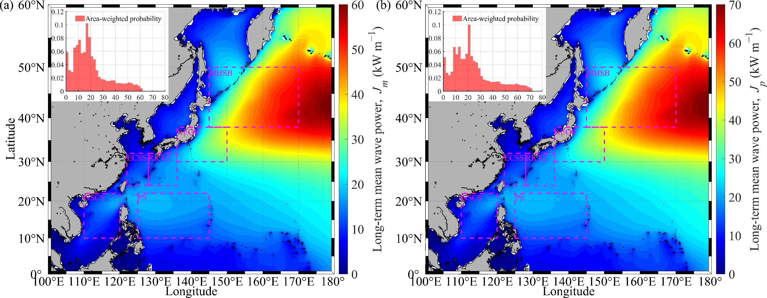
Figure 1. Long-term mean wave-power density in the Northwest Pacific estimated using (a) the mean-period-based formulation, Jm = 0.49$${\textit{H}}_{\textit{s}}^{\text{2}}$$Tm, and (b) the peak-period-based sensitivity formulation, Jp = 0.49$${\textit{H}}_{\textit{s}}^{\text{2}}$$Tp. Insets show latitude-weighted probability distributions of grid-cell long-term mean wave power. Magenta dashed boxes denote the six diagnostic subregions.
The area-weighted probability distributions embedded in Figure 1a further show that the basin is not dominated by uniformly high wave power. For Jm, the distribution is strongly right skewed, with the highest area-weighted probabilities concentrated around 10–20 kW·m−1. The modal bin occurs near 16–20 kW·m−1, where the area-weighted probability reaches approximately 0.10–0.11. By contrast, grid cells exceeding 40 kW·m−1 form a much smaller fraction of the basin area, appearing as a long high-energy tail rather than the dominant resource class. The most energetic region east of Japan is therefore spatially prominent but not representative of the Northwest Pacific as a whole. The basin-scale resource distribution consists primarily of low- to moderate-power environments and a relatively limited but intense high-power storm-belt sector.
The sensitivity estimate based on peak wave period, Jp, preserves the same spatial pattern but increases wave-power magnitude throughout the basin (Figure 1b). The high-energy core east of Japan remains the dominant resource center, and the relative ranking among the subregions is essentially unchanged. However, the color scale and histogram indicate a systematic upward shift in magnitude: the Jp field reaches approximately 65–70 kW·m−1, compared with 55–60 kW·m−1 for Jm. The area-weighted distribution of Jp is similarly right skewed but shifted toward higher values, with its modal range closer to approximately 18–22 kW·m−1. This behaviour is expected because Tp is generally longer than the mean-period proxy used in Jm. Therefore, Jp is interpreted as an upper sensitivity estimate rather than an alternative resource climatology.
The comparison between Jm and Jp has two implications. First, the spatial structure of the resource is robust to the choice of period proxy: the same high-resource and low-resource regions emerge under both estimates. Second, the absolute magnitude is sensitive to the selected wave-period parameter, supporting the use of Jm as a conservative principal estimate and Jp as a sensitivity reference. This is consistent with wave-energy assessment guidance, which emphasizes that the energy period is the preferred characteristic period but that proxy-based estimates should explicitly document uncertainty when Te is unavailable. In the present study, period-proxy uncertainty changes the estimated resource magnitude but not the basin-scale interpretation: the Northwest Pacific contains a pronounced high-power regime east of Japan and within the storm belt, while most marginal and shelf seas remain moderate or weak in terms of long-term mean wave power.
The seasonal mean fields reveal that the long-term mean resource pattern shown in Figure 1 is primarily shaped by winter conditions (Figure 2a,b). During DJF, wave power is strongly amplified over the open Northwest Pacific, especially east of Japan and within the MHSB. The DJF mean Jm exceeds 80 kW·m−1 over a broad sector east of 155° E and reaches local maxima of approximately 110–120 kW·m−1 in the eastern part of the domain. The high-energy core extends southwestward toward the KEOR, where winter mean wave power commonly reaches 40–70 kW·m−1. This indicates that the KEOR acts as a transition zone between the lower-resource western-boundary and shelf seas and the fully exposed mid-latitude storm-belt regime.
By contrast, marginal seas and shelf regions remain much weaker in winter. The ECSS generally exhibits DJF mean wave power below 15–20 kW·m−1, whereas most of the NSCS remains below 20 kW·m−1, except for localized enhancement along exposed coastal and island-margin sectors. The PS and RKTZ occupy intermediate conditions. In the PS, winter wave power is mostly approximately 20–30 kW·m−1, whereas the RKTZ shows a sharper spatial gradient from relatively weak values near the East China Sea shelf to stronger values east of the Ryukyu Arc. This contrast supports the interpretation that exposure to open-ocean storm waves, rather than latitude alone, strongly shapes the winter resource distribution.
The JJA field is much weaker and spatially smoother than the DJF field. Most of the open Northwest Pacific decreases to approximately 10–20 kW·m−1, with only limited areas exceeding 20 kW·m−1. The strongest summer values occur in a subtropical band extending from the Philippine Sea toward the waters east of Taiwan and south of Japan, where JJA mean Jm locally approaches 20–30 kW·m−1. In the MHSB and KEOR, however, the summer reduction is substantial: regions exceeding 60–100 kW·m−1 in DJF mostly decrease to below 20 kW·m−1 in JJA. This confirms that the highest-resource sector is strongly seasonal and dominated by winter storm-wave conditions rather than a persistent year-round energy supply.
The DJF–JJA difference field in Figure 2c highlights this seasonality more directly. Across the eastern and mid-latitude open Northwest Pacific, DJF exceeds JJA by more than 40 kW·m−1, with the difference reaching approximately 70–100 kW·m−1 in the storm-belt high-energy core. The largest winter–summer contrast is therefore colocated with the long-term high-resource center in Figure 1. This result is relevant to resource-quality assessment because the region with the largest mean wave power is also the region in which the annual resource depends most strongly on winter enhancement. Thus, the high-power regime east of Japan is not only energetic but also strongly seasonal.
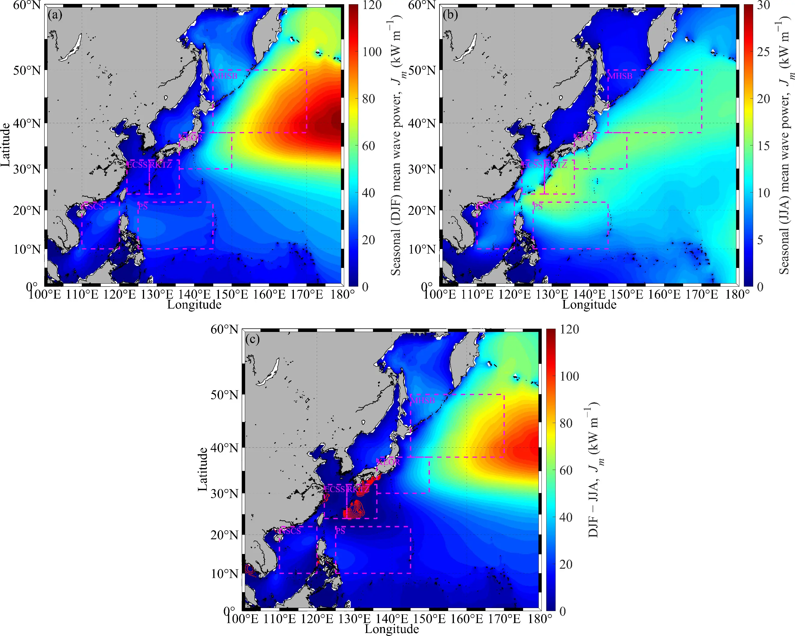
Figure 2. Seasonal mean Jm during (a) DJF and (b) JJA, and (c) the DJF–JJA difference. Red contours in (c) identify locally summer-dominant conditions; magenta dashed boxes denote the six diagnostic subregions.
The red contours in the DJF–JJA panel mark areas where Jm,DJF − Jm,JJA < 0, indicating that summer wave power locally exceeds winter wave power. These negative-difference zones are small compared with the winter-dominant open-ocean area, but they are physically meaningful. One such region appears within or near the RKTZ, where the summer resource can locally exceed the winter value. This suggests that parts of the Ryukyu–Kuroshio transition are influenced by summer wave systems, possibly associated with tropical-cyclone activity, subtropical swell, and western Pacific wave propagation. Smaller negative-difference areas also appear along parts of the East China coastal margin and the southwestern coast of Southeast Asia, including coastal waters near Vietnam and Cambodia. These coastal and marginal-sea anomalies indicate that local monsoonal wind regimes, tropical disturbances, and coastal exposure can locally reverse the basin-scale winter-dominant pattern.
This seasonal pattern is consistent with the broader climatology of the Northwest Pacific. In winter, intensified extratropical cyclones and stronger East Asian monsoon winds enhance wave generation over the mid-latitude western North Pacific. In summer, the storm track weakens and shifts, reducing background wave power over the MHSB and KEOR, while tropical-cyclone and monsoon-related wave activity becomes more relevant in subtropical and marginal seas. Previous wave-climate and wave-energy studies have similarly emphasized that mid-latitude storm forcing and monsoonal variability strongly shape seasonal wave resources in the western North Pacific and China’s adjacent seas [7,19,20,21,22,23,24]. The present result extends this interpretation by showing that seasonal forcing not only modulates resource magnitude but also structures the resource-quality problem by separating winter-amplified high-power regions from more moderate and potentially less seasonally concentrated regions.
The subregional monthly cycles in Figure 3a–f provide a quantitative view of the seasonal contrasts identified in Figure 2, separating the basin into a winter-dominant storm-wave regime, a summer–autumn-enhanced transition regime, and lower-energy marginal-sea regimes. The storm-dominated MHSB and KEOR exhibit the largest seasonal amplitudes. The MHSB peaks in winter, exceeding 70 kW·m−1, and decreases to approximately 10–15 kW·m−1 in summer, emphasizing its high-energy but highly variable character. Conversely, the marginal-sea and transition regions—PS, RKTZ, ECSS, and NSCS—have substantially lower gross resource intensity but exhibit distinct and, in some cases, complementary seasonal behavior. For example, the RKTZ and ECSS exhibit late-summer and autumn resource plateaus associated with tropical-cyclone activity and subtropical swell, avoiding the extreme winter–summer contrast of the northern storm-belt regions. These temporal differences indicate that lower-annual-mean regions may provide seasonal availability when storm-belt resources are near their annual minima.
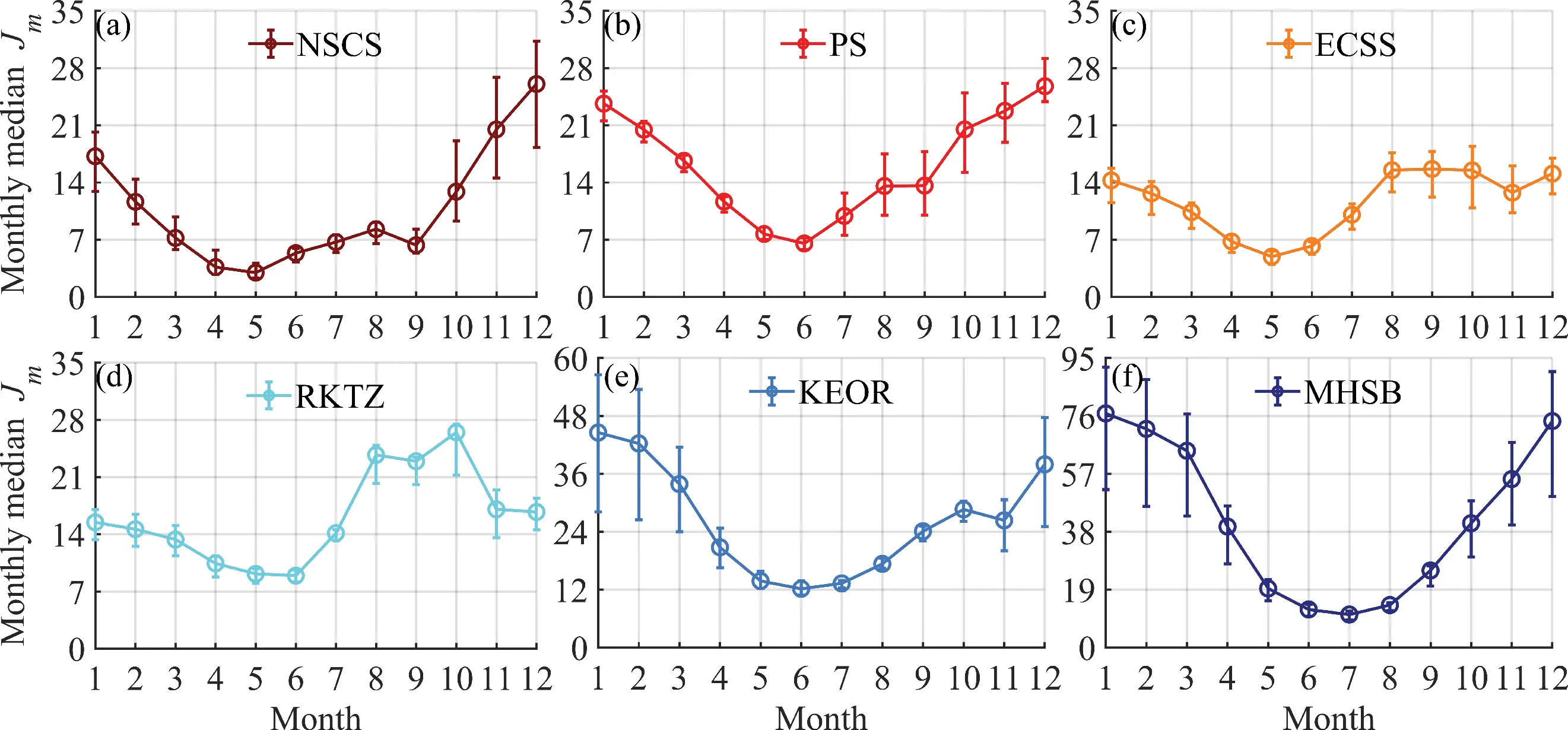
Figure 3. Monthly evolution of median Jm in (a) NSCS, (b) PS, (c) ECSS, (d) RKTZ, (e) KEOR, and (f) MHSB. Circles denote monthly medians, and vertical bars show the interquartile range across grid cells. The vertical-axis range differs among panels.
The NSCS has the lowest springtime resource but a strong late-year increase (Figure 3a). Median Jm decreases from 17 kW·m−1 in January to approximately 3–5 kW·m−1 in April–May, gradually recovers through summer, and rises sharply after October, reaching approximately 20 kW·m−1 in November and 25–27 kW·m−1 in December. This cycle is consistent with winter-monsoon enhancement over the northern South China Sea, with a secondary warm-season contribution that may be linked to regional monsoon and tropical-storm activity. The NSCS, therefore, has a low annual mean compared with the open-ocean regions, but its December–January resource can briefly reach levels comparable to or higher than the annual medians of some transition regions. Together, these monthly curves clarify an important point that is less visible in the maps alone: the spatial ranking of wave-energy intensity changes with season. The MHSB and KEOR dominate the basin in winter but lose much of their advantage in summer. The RKTZ and ECSS strengthen during late summer and autumn, whereas the NSCS exhibits a pronounced winter-monsoon peak despite low spring values. The monthly cycles, therefore, support the distinction between resource intensity and resource quality. The highest-resource regions have the strongest seasonal concentration, whereas some moderate-resource regions display different seasonal timing or less extreme annual contrasts. This temporal complementarity is relevant to basin-scale planning because a region with lower annual mean wave power may still provide valuable seasonal availability, particularly if its energetic months do not coincide with the summer minima of the storm-belt regions.
The upper-tail wave-power fields further confirm that the energetic core of the Northwest Pacific is concentrated east of Japan and within the mid- to high-latitude storm belt (Figure 4a,b). The conditional mean wave power above the local 90th percentile, $$\overline{J_m \mid J_m > P90}$$, broadly follows the long-term mean pattern in Figure 1, but with a much sharper contrast between the open-ocean storm-belt sector and the marginal seas. In the MHSB and the eastern part of the domain, $$\overline{J_m \mid J_m > P90}$$ commonly exceeds 160 kW·m−1, with local maxima approaching 220–240 kW·m−1. The KEOR also shows elevated upper-tail resources, generally around 80–160 kW·m−1, indicating that this transition region is frequently affected by energetic winter and storm-wave conditions. By contrast, the NSCS, ECSS, and most shelf seas remain mostly below 50–90 kW·m−1, except for locally exposed areas near Taiwan, the Ryukyu Arc, and parts of the western Pacific margin. The conditional mean above the local 99th percentile, $$\overline{J_m \mid J_m > P99}$$, reveals an even stronger concentration of extreme resource intensity in the open Northwest Pacific. Marginal and shelf regions such as the ECSS and NSCS remain lower overall, although localized enhancement occurs around exposed island chains and shelf-break transition zones.
The subregional pattern is consistent with the seasonal cycles in Figure 3. The MHSB, with its large winter maximum and strong seasonal amplitude, also exhibits the highest upper-percentile wave power. The KEOR behaves as a secondary high-tail region, reflecting its exposure to winter storm waves and the western-boundary-current extension environment. The PS and RKTZ have lower mean resources than the MHSB, but their upper-tail values remain non-negligible, suggesting occasional energetic events associated with western Pacific swell, tropical cyclones, or transition-season wave systems. The ECSS and NSCS show weaker upper-tail resources, but their localized high-percentile enhancement near exposed coasts and island passages indicates that marginal seas can still experience episodic high-energy conditions despite low basin-scale means.
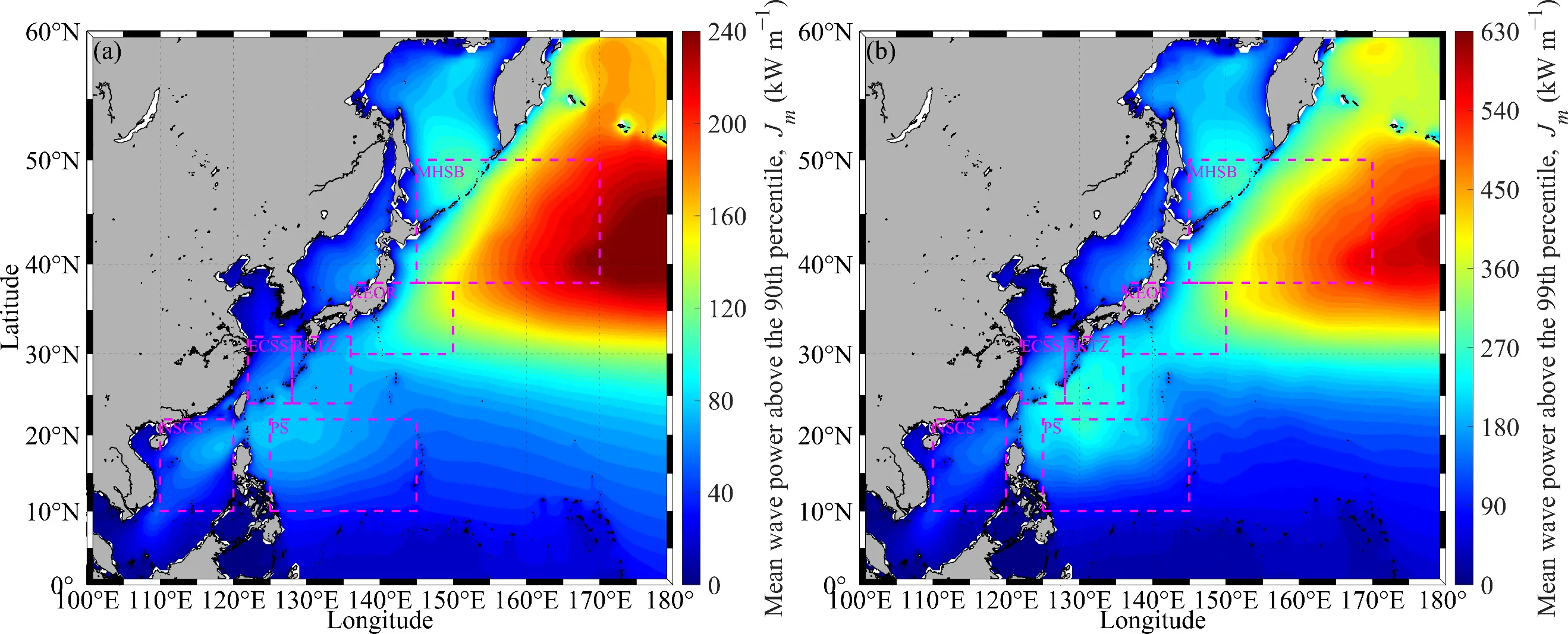
Figure 4. Upper-tail wave-power intensity: conditional mean Jm above the local (a) 90th and (b) 99th percentiles. Percentile thresholds were calculated independently at each grid cell. Magenta dashed boxes denote the six diagnostic subregions.
The joint Hs–Tm frequency matrices provide a sea-state-level explanation for the spatial and seasonal resource patterns described above (Figure 5a–g). For the full Northwest Pacific, the most frequent sea states are concentrated around moderate wave heights and periods, with a dominant cluster near Hs ≈ 1.2–2.0 m and Tm ≈ 6.5–8.5 s. This cluster lies mostly between the 5 and 20 kW·m−1 wave-power contours, indicating that the basin-wide wave climate is dominated by moderate-energy sea states rather than persistently extreme conditions. However, the distribution has a clear upper-right tail toward larger Hs and longer Tm, crossing the 20 and 40 kW·m−1 contours. This tail is small in frequency but important for the high-percentile resource fields shown in Figure 4.
The marginal-sea subregions show distinctly lower-energy sea-state structures. In the NSCS, the highest-frequency states are centered around Hs ≈ 0.5–1.4 m and Tm ≈ 4–6.5 s, with most of the distribution falling below or near the 5–10 kW·m−1 contours. The distribution is elongated along a positive Hs–Tm direction, suggesting that higher waves are accompanied by longer periods, but the majority of sea states remain relatively low in wave-power density. The ECSS is similar but slightly more compact, with its frequency maximum near Hs ≈ 0.8–1.5 m and Tm ≈ 4.5–6.5 s. Most ECSS sea states remain below 10 kW·m−1, consistent with the low-to-moderate mean and upper-percentile resources shown in Figure 1 and Figure 4. These two regions therefore represent marginal-sea regimes in which frequent sea states are relatively mild and of short period, even though episodic storm or monsoon events can still produce higher-energy tails.
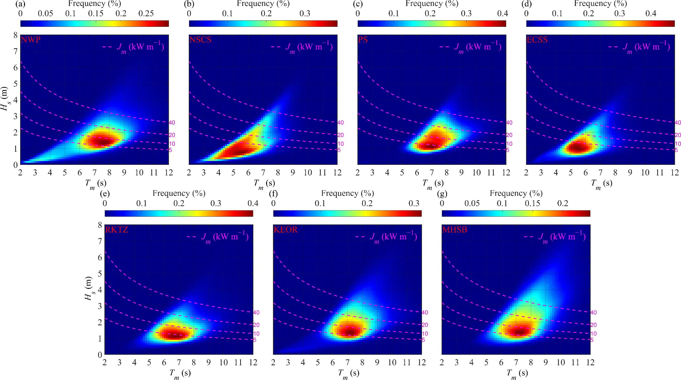
Figure 5. Joint Hs–Tm frequency distributions for (a) the Northwest Pacific and (b–g) the six diagnostic subregions. Magenta contours denote Jm in kW·m−1; color scales differ among panels.
The PS and RKTZ occupy intermediate positions between the marginal seas and high-energy open-ocean regions (Figure 5c,e). In the PS, the dominant frequency lobe is shifted toward longer periods and is centered around Hs ≈ 0.9–2.0 m and Tm ≈ 6–8 s. This places a substantial proportion of the frequent sea states between the 5 and 20 kW·m−1 contours. The RKTZ shows a comparable but slightly lower-energy distribution, with the most frequent states around Hs ≈ 0.9–1.6 m and Tm ≈ 5.5–7.5 s. The longer-period character of the PS and RKTZ relative to the NSCS and ECSS is consistent with their greater exposure to open-ocean swell and western Pacific wave systems. It also helps explain why these regions can show moderate resource levels even when their wave heights are not as large as those in the storm belt: longer periods partly compensate for moderate Hs in the wave-power calculation.
The KEOR and MHSB exhibit the clearest open-ocean high-energy signatures (Figure 5f,g). In the KEOR, the main frequency concentration occurs around Hs ≈ 1.2–2.0 m and Tm ≈ 6–8 s, but the distribution extends more strongly toward Hs > 3 m and Tm > 8 s than in the lower-latitude regions. An appreciable proportion of the KEOR sea-state space therefore reaches the 20–40 kW·m−1 contours. The MHSB has the broadest and most energetic distribution among all subregions. Its frequent states are shifted toward higher wave heights, approximately Hs ≈ 1.2–2.3 m and Tm ≈ 6.5–8.5 s, and its upper tail extends toward Hs ≈ 4–5 m and Tm ≈ 9–10 s. This places a much larger part of the distribution near or above the 20 kW·m−1 contour, with extreme tail states reaching or exceeding 40 kW·m−1. These sea-state characteristics explain why the MHSB dominates both the long-term mean resource and the upper-percentile resource maps.
The subregional matrices also provide physical insight into the source regimes discussed later. Shorter-period, lower-height clusters in the NSCS and ECSS are consistent with locally generated wind sea and monsoon-influenced shelf-sea conditions. Longer-period, moderate-height clusters in the PS and RKTZ suggest stronger swell influence and open-ocean exposure. The broader high-Hs, long-Tm tail in the KEOR and MHSB is characteristic of storm-generated open-ocean wave systems and extratropical wave growth. This interpretation is consistent with established wind-sea/swell partitioning concepts and global wave-climate studies that distinguish locally forced wind seas from remotely generated swell fields [16,17,18].
The Jm–Tm contribution matrices further demonstrate that the most frequent sea states are not necessarily the dominant contributors to total wave power (Figure 6a–g). For the full Northwest Pacific, the largest contribution to accumulated wave power is concentrated around Tm ≈ 6.5–8.5 s and Jm ≈ 5–25 kW·m−1, although the contribution field extends upward to Jm > 60 kW·m−1. Compared with the Hs–Tm frequency distribution in Figure 5a, the energy-contribution maximum is shifted toward higher wave-power classes. This confirms that moderate-to-energetic sea states, rather than the most frequently occurring low-energy states, dominate the basin-integrated wave-energy budget.
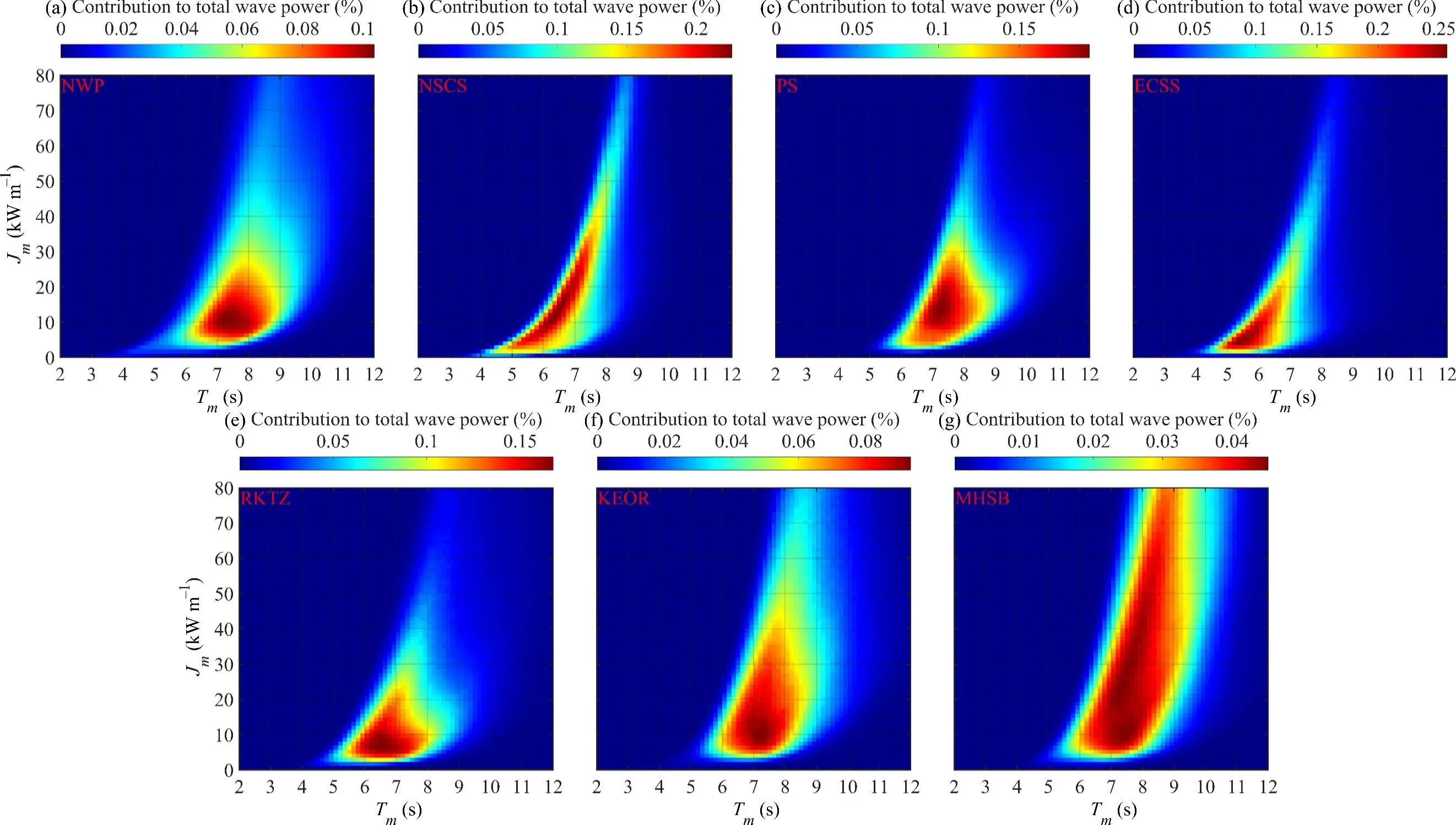
Figure 6. Contributions of Jm–Tm bins to total wave power for (a) the Northwest Pacific and (b–g) the six diagnostic subregions. Color scales differ among panels.
The marginal-sea regions show relatively narrow and low-power contribution structures. In the NSCS, most of the contribution is concentrated along a curved band from Tm ≈ 5–7.5 s and Jm ≈ 3–35 kW·m−1, with the highest contribution occurring around Tm ≈ 6–7 s and Jm ≈ 8–25 kW·m−1. Although the most frequent sea states in Figure 5b are located at lower Hs and shorter periods, Figure 6b shows that the energetic contribution is displaced upward toward stronger monsoon- or storm-related conditions. This indicates that the NSCS resource is not controlled by the background low-energy sea state but by intermittent moderate-energy events. The ECSS has a still lower-energy contribution structure. Its dominant contribution is concentrated mainly around Tm ≈ 5–6.5 s and Jm ≈ 3–18 kW·m−1, with only a limited extension toward Jm ≈ 20–30 kW·m−1. This agrees with the low annual mean and upper-percentile resources observed in Figure 1 and Figure 4. The compactness of the ECSS contribution matrix suggests that relatively short-period and moderate-power conditions dominate this shelf region. Even when energetic events occur, their contribution remains much smaller than in open-ocean transition and storm-belt regions.
The PS and RKTZ occupy intermediate positions in both period and wave-power contribution. In the PS, the main contribution is centered near Tm ≈ 6.5–8.5 s and Jm ≈ 6–30 kW·m−1, with a moderate upward extension beyond 40 kW·m−1. This pattern indicates that the PS resource benefits from longer-period wave systems, even though its wave heights are not as large as those in the storm belt. The RKTZ contribution maximum is slightly lower, mainly around Tm ≈ 6–7.5 s and Jm ≈ 5–25 kW·m−1, but it also extends toward higher power classes. Together, these two regions represent transition regimes in which moderate wave heights combined with relatively long periods generate evident wave-energy contributions.
The KEOR and MHSB exhibit the most energetic contribution structures. In the KEOR, the dominant contribution occurs around Tm ≈ 6.5–8 s and Jm ≈ 5–35 kW·m−1, with a clear extension to Jm > 60 kW·m−1. This indicates that the KEOR is not merely a moderate-frequency transition zone; it also receives substantial contributions from episodic high-power sea states. The MHSB shows the broadest and most vertically extended contribution matrix among all subregions. Its main contribution band spans Tm ≈ 7–9 s and Jm ≈ 5–65 kW·m−1, with high contributions distributed over a wide range of energetic states. This broad vertical structure explains why the MHSB dominates both the mean wave-power map and the upper-tail statistics: its energy budget is supported not only by frequent moderate-power conditions but also by repeated high-power events.
The contrast between Figure 5 and Figure 6 is central to interpreting wave-energy resource quality. In the Hs–Tm frequency matrices, the highest occurrence probabilities are often found in mild or moderate sea states. However, because Jm scales with $${\textit{H}}_{\textit{s}}^{\text{2}}$$Tm, relatively infrequent increases in wave height can dominate the accumulated energy contribution. This is most evident in the KEOR and MHSB, where the contribution maxima extend far above the most frequent background sea states. In contrast, the NSCS and ECSS contain frequent sea states but relatively limited high-power contributions. Thus, an assessment based only on sea-state occurrence would underestimate the importance of energetic tails, whereas an assessment based only on mean power would fail to distinguish whether persistent moderate states or intermittent high-power events supply the resource.
Physically, the contribution structures reflect different wave-generation regimes. The compact, low-power contribution fields in the ECSS and NSCS are consistent with marginal-sea and shelf environments where local monsoon forcing, limited fetch, shallow-water effects, and coastal sheltering constrain wave growth. The PS and RKTZ exhibit longer-period contribution bands, consistent with stronger open-ocean swell influence and exposure to western Pacific wave propagation. The KEOR and MHSB show broader high-power tails, reflecting their exposure to extratropical storm waves and winter storm-track activity. This interpretation is consistent with wind-sea/swell climate studies showing that locally generated wind seas and remotely generated swells form distinct wave systems with different variability and propagation characteristics [16,17,18].
Although the long-term mean and upper-tail wave-power distributions establish the theoretical energy intensity of the Northwest Pacific, these time-averaged metrics do not fully reflect the realistic operational conditions experienced by wave energy converters. High mean power may be disproportionately influenced by severe, intermittent storm events rather than by a consistent energy flux. Evaluating the practical viability of these regions, therefore, requires explicit consideration of temporal stability and continuous availability.
3.2. Temporal Stability and Availability of Wave-Energy Resources
The stability diagnostics show that the spatial pattern of wave-energy quality differs markedly from that of wave-energy intensity (Figure 7). Whereas Figure 1, Figure 2, Figure 3, Figure 4, Figure 5 and Figure 6 identify the MHSB and KEOR as the principal high-power regimes, Figure 7a–d demonstrates that high wave power is often accompanied by strong temporal variability. This confirms that resource intensity alone is insufficient for evaluating practical wave-energy potential and that monthly, seasonal, and interannual fluctuations must be considered jointly, as recommended in wave-energy resource-assessment guidance and review studies [12,13,14,15].
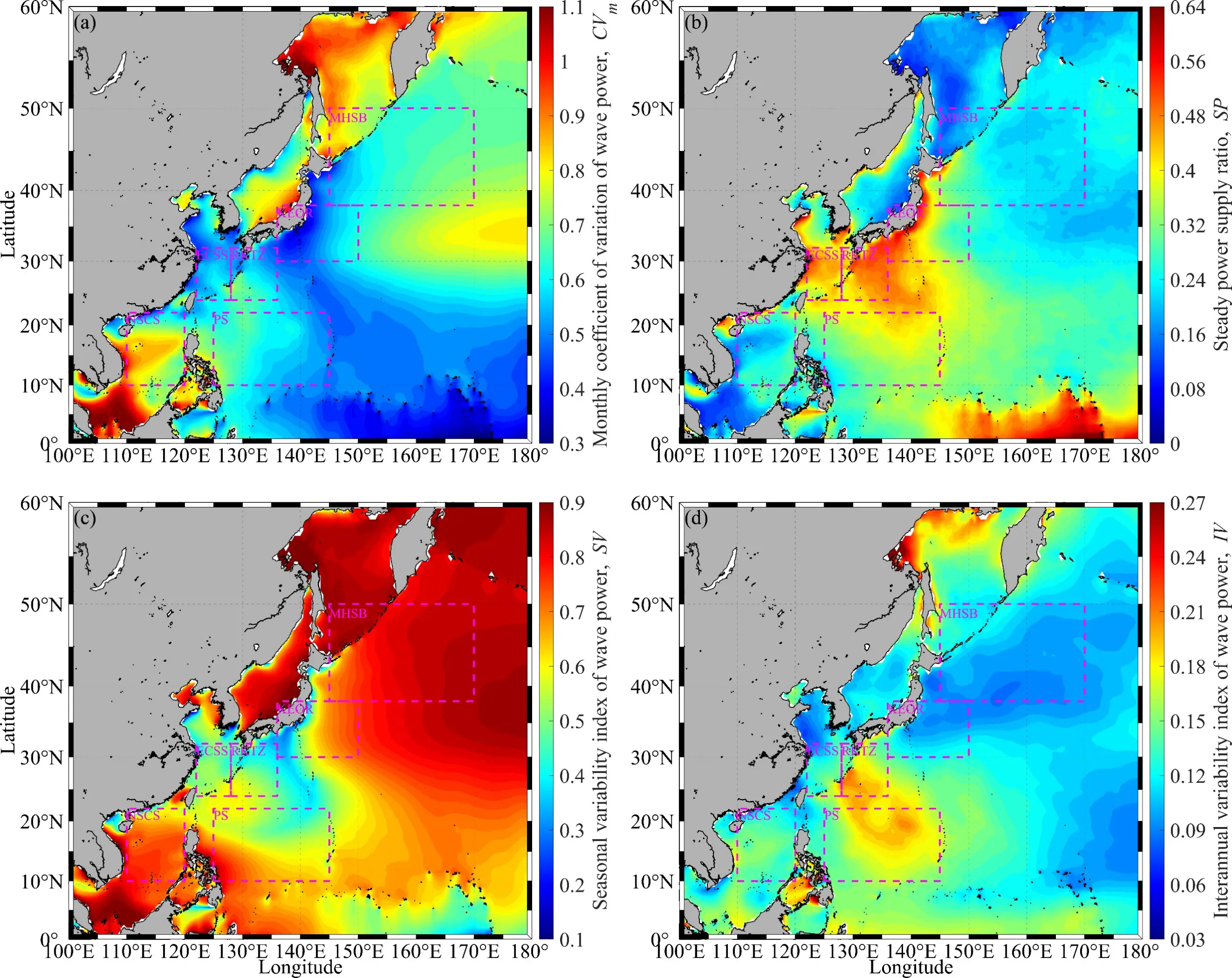
Figure 7. Wave-energy variability metrics: (a) monthly coefficient of variation CVm, (b) steady-power-supply ratio SP, (c) seasonal variability SV, and (d) interannual variability IV. Magenta dashed boxes denote the six diagnostic subregions.
The monthly coefficient of variation, CVm, shows the relative amplitude of month-to-month variability (Figure 7a). Low CVm values of approximately 0.3–0.5 occur mainly in parts of the tropical-to-subtropical open Northwest Pacific, particularly in and around the PS, RKTZ, and parts of the open ocean southeast of Japan. These areas have lower absolute resource intensity than the storm belt but exhibit comparatively smooth monthly fluctuations. In contrast, CVm exceeds 0.8 in several marginal and high-latitude regions, including the northern South China Sea, coastal Southeast Asian waters, the Japan Sea–Okhotsk sector, and parts of the northern margin of the MHSB. In these areas, the standard deviation of monthly wave power is comparable to or greater than the mean monthly resource, indicating strong intermittency. The MHSB itself exhibits moderate-to-high CVm, commonly around 0.5–0.7 in the open-ocean sector and higher values near its northern and western margins. This pattern is consistent with the strong winter maximum and summer minimum shown in Figure 2 and Figure 3.
The steady-power-supply ratio, SP, provides a complementary view (Figure 7b). Unlike CVm, which measures variability amplitude, SP measures how frequently monthly wave power remains close to its long-term reference level. High SP values, reaching approximately 0.48–0.64, occur mainly along parts of the East China Sea shelf, the waters around Japan, and several western-boundary or shelf-transition regions. These regions do not always have the highest mean wave power, but their monthly values are more frequently maintained within the prescribed stable range. By contrast, lower SP values, mostly below 0.32, occur over large parts of the MHSB and high-latitude marginal regions. This indicates that the storm-belt resource, although energetic, often departs substantially from its annual mean. The contrast between CVm and SP highlights an inverse resource-quality pattern: a region can be energetic but unstable, whereas another region can be moderate in magnitude but more favorable in terms of monthly steadiness.
The seasonal variability index, SV, exhibits the clearest large-scale contrast among the four stability diagnostics (Figure 7c). Values above 0.7 dominate much of the mid- to high-latitude open Northwest Pacific, especially the MHSB and the waters east of Japan. The KEOR also exhibits elevated SV, generally around 0.6–0.8. These values reflect the large winter–summer contrast shown in Figure 2, where DJF wave power exceeds JJA wave power by tens of kW·m−1 over the open ocean. The NSCS and some coastal Southeast Asian waters also exhibit high SV, locally reaching 0.7–0.9, consistent with strong monsoon-season modulation. In contrast, the lowest SV values, approximately 0.3–0.5, occur over parts of the subtropical Philippine Sea and transition zones where the annual cycle is less dominated by a single winter maximum. This supports the interpretation that moderate-resource regions can sometimes provide more seasonally balanced resources than the strongest storm-belt areas.
The interannual variability index, IV, has a much smaller numerical range than CVm, mostly between 0.03 and 0.27, but it reveals a different spatial structure (Figure 7d). The lowest IV values, generally below 0.10–0.12, occur over broad parts of the open Pacific, including portions of the PS, KEOR, and MHSB. This suggests that, despite strong seasonal cycles, the year-to-year mean resource in parts of the open ocean is relatively stable compared with its seasonal variability. Higher IV values, approximately 0.18–0.27, occur in several western-boundary and marginal regions, including waters east of Taiwan and the Philippines, parts of the East China Sea–Ryukyu transition, and the high-latitude marginal seas. These areas are more likely to be affected by interannual variations in monsoon intensity, tropical cyclone activity, storm-track position, and regional circulation patterns. Thus, the strongest year-to-year uncertainty is not necessarily colocated with the highest mean wave power.
These four diagnostics demonstrate that a single metric cannot accurately represent wave-energy stability. The MHSB has the largest resource intensity, but it also exhibits high seasonal variability and relatively low monthly steadiness. The KEOR behaves as a high-resource transition region, with strong seasonal modulation but comparatively moderate interannual variability. The PS and RKTZ show lower mean wave power but more moderate CVm, weaker seasonal contrast, and locally higher monthly steadiness, suggesting a more persistent resource character. The NSCS and ECSS remain lower-resource regions, but their stability structures differ: the NSCS is strongly affected by seasonal monsoon modulation, whereas parts of the ECSS and nearby shelf-transition waters show relatively high SP, indicating steadier monthly behavior despite modest resource intensity.
The availability diagnostics provide an operational perspective that is not captured by mean wave power alone (Figure 8a–d). Here, A10 represents the fraction of six-hourly records for which Jm > 10 kW·m−1 and therefore measures how often a grid cell exceeds a moderate wave-power threshold. Compared with the variability metrics in Figure 7, A10 translates the resource climate into a more direct indicator of potential operating time. The spatial patterns show that the Northwest Pacific contains both highly available but strongly seasonal open-ocean resources and lower-availability marginal-sea resources.
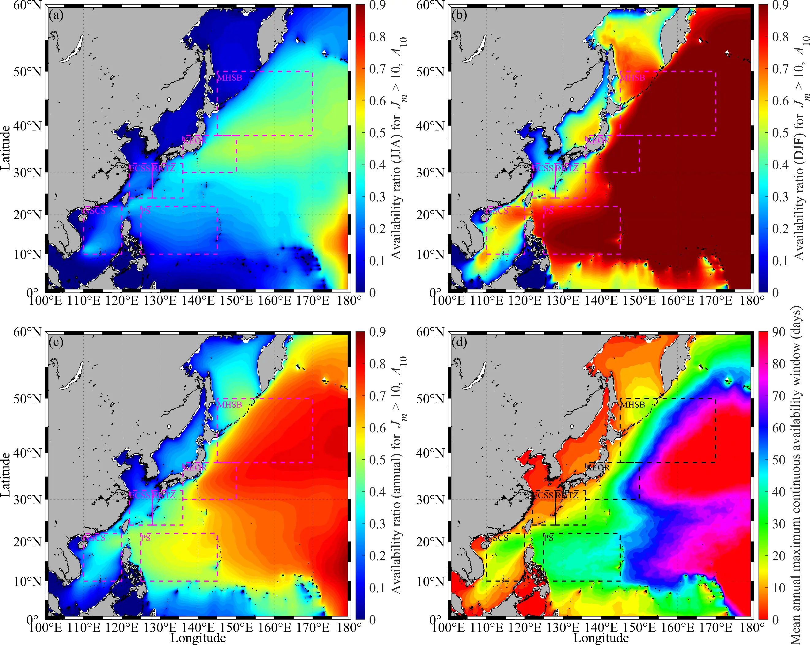
Figure 8. Availability and persistence of wave-power conditions exceeding 10 kW·m−1: (a) JJA A10, (b) DJF A10, (c) annual A10, and (d) mean annual maximum continuous availability window. Magenta dashed boxes denote the six diagnostic subregions.
The JJA availability field is relatively weak over most of the basin (Figure 8a). In the Yellow Sea, Japan Sea, and western marginal seas, A10 generally remains below 0.2, indicating that fewer than 20% of summer six-hourly records exceed 10 kW·m−1. The NSCS and ECSS also exhibit low summer availability over most of their areas, although exposed local sectors can reach approximately 0.2–0.4. By contrast, the open Pacific east and southeast of Japan maintains moderate summer availability, commonly around 0.3–0.5, with locally higher values near the eastern and southeastern margins of the domain. This suggests that even during the basin-wide summer minimum identified in Figure 2 and Figure 3, some open-ocean swell or tropical and subtropical wave systems continue to support moderate wave-power availability.
The DJF availability field is markedly different (Figure 8b). A broad region east of Japan, extending through the KEOR into the MHSB and open Northwest Pacific, exhibits A10 > 0.7, with large areas approaching 0.8–0.9. During winter, more than 70–90% of six-hourly records in these open-ocean regions therefore exceed the 10 kW·m−1 threshold. This is consistent with the high DJF wave power shown in Figure 2 and the winter maxima in Figure 3. The winter availability enhancement is particularly strong in the MHSB and KEOR, confirming that these regions are not only high-power sectors but also high-availability sectors during the energetic season. However, the same pattern also implies strong seasonal dependence: the operationally favorable period is concentrated in winter rather than distributed evenly throughout the year.
The annual A10 field integrates these seasonal contrasts (Figure 8c). The highest annual availability occurs in the open Northwest Pacific east of Japan, where A10 generally exceeds 0.6 and locally approaches 0.8–0.9. The KEOR and MHSB, therefore, remain the most available regions on an annual basis despite their strong seasonality. The PS and RKTZ show intermediate annual availability, mostly around 0.3–0.6, indicating that moderate resources occur frequently enough to maintain meaningful operating potential. The NSCS and ECSS generally exhibit lower annual availability, commonly below 0.2–0.4, although localized enhancement occurs along exposed coastlines, island margins, and transition zones. These results are consistent with the resource-intensity hierarchy in Figure 1, Figure 2, Figure 3, Figure 4, Figure 5 and Figure 6, but they also sharpen the interpretation: high mean power is most meaningful when it translates into a high exceedance fraction, and this translation is strongest over the open ocean.
The maximum continuous availability window adds a persistence dimension to the threshold exceedance analysis (Figure 8d). Whereas A10 measures the total fraction of available time, the continuous-window metric identifies whether available conditions occur as sustained intervals or fragmented short events. The longest windows are concentrated in the central and eastern open Northwest Pacific, especially east of Japan and within the offshore part of the MHSB, where the mean annual maximum continuous window ranges from approximately 60 to 90 days. This indicates that winter high-power conditions can persist for several months in the open-ocean storm-belt regime. The KEOR and adjacent open waters generally show intermediate-to-high persistence, with windows of approximately 30–70 days. In contrast, marginal seas and coastal shelf regions, including much of the NSCS, ECSS, Japan Sea, and sheltered coastal waters, mostly show much shorter windows, commonly below 5–30 days. Their exceedance events are therefore more intermittent, even when localized seasonal or storm-related enhancement occurs. Physically, these patterns reflect the combined influence of the winter extratropical storm track, the East Asian winter monsoon, and open-ocean swell propagation. The winter storm-belt regime generates persistent high-energy waves east of Japan, explaining the high DJF A10 and long continuous windows. In summer, weakened mid-latitude storm activity reduces the availability of high-power conditions in the MHSB and KEOR. Tropical cyclones and monsoonal forcing can locally enhance summer and autumn wave power, but these events are more spatially and temporally intermittent.
The monthly evolution of A10 further quantifies the seasonal availability patterns shown in Figure 8 (Figure 9a–f). The strongest winter availability occurs in the MHSB. Monthly median A10 is close to 1.0 from December to February and remains above 0.85 in March and April, indicating that almost all six-hourly records exceed 10 kW·m−1 during the energetic season. However, A10 decreases rapidly after spring, reaching approximately 0.35–0.40 in June–July before increasing again after August. This behavior mirrors the strong winter maximum and summer minimum of Jm in Figure 3, but it also shows that the MHSB retains some moderate availability during its seasonal minimum. The MHSB therefore, represents a high-availability but strongly seasonal regime. The KEOR shows a similar but slightly less pronounced seasonal evolution. Median A10 is approximately 0.90–0.95 during December–February, decreases to 0.35–0.40 in June–July, and then recovers to 0.70–0.90 from October to December. Compared with the MHSB, the KEOR has lower winter wave-power intensity, but its winter availability is similarly high because the 10 kW·m−1 threshold is exceeded during most winter records. This contrast is important: once a region frequently exceeds a moderate threshold, A10 becomes less sensitive to the magnitude by which the threshold is exceeded. Thus, the KEOR and MHSB may both exhibit high winter availability yet differ substantially in resource magnitude and high-energy exposure.
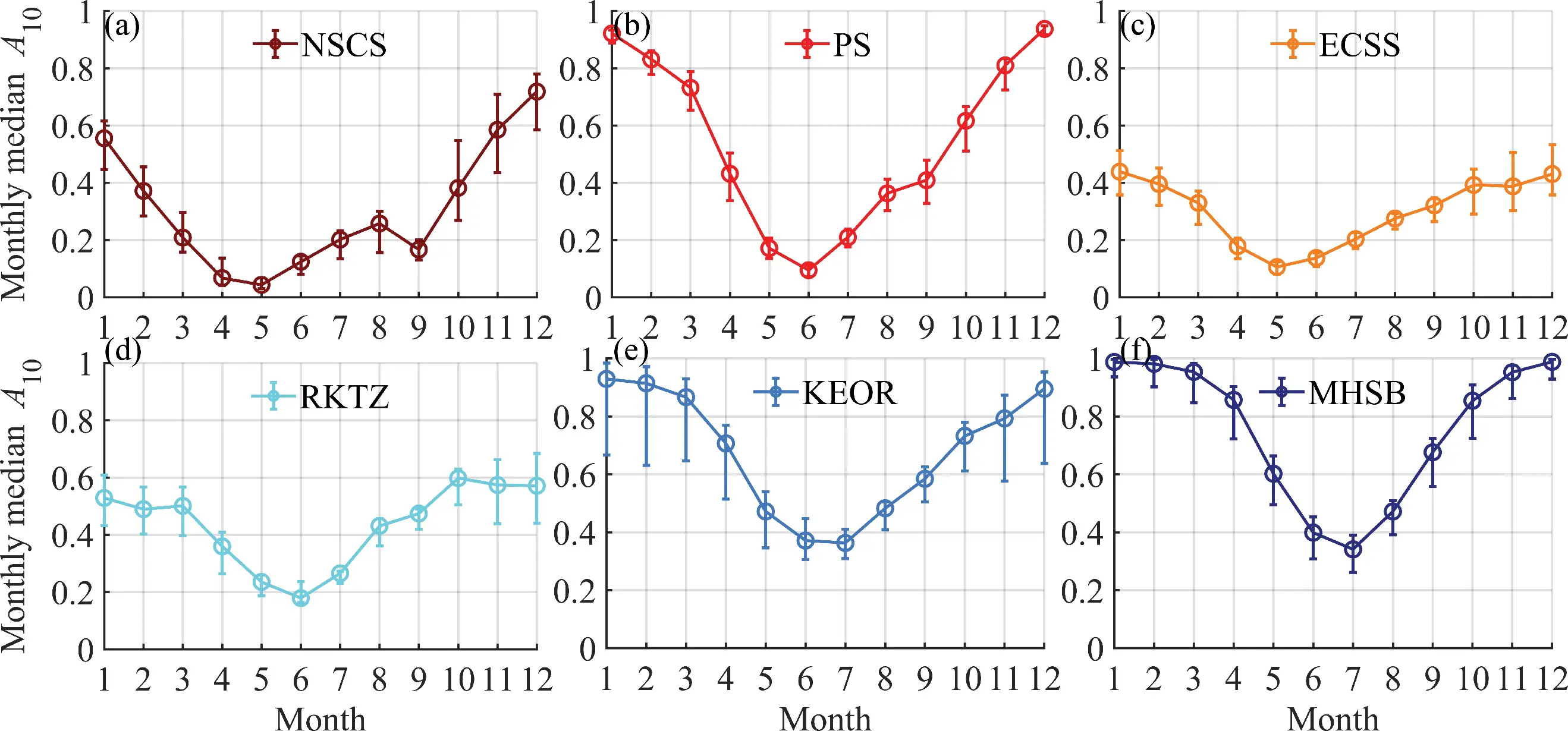
Figure 9. Monthly evolution of median A10 in (a) NSCS, (b) PS, (c) ECSS, (d) RKTZ, (e) KEOR, and (f) MHSB. Circles denote monthly medians, and vertical bars show the interquartile range across grid cells.
The PS also exhibits high winter availability, with median A10 around 0.90 in January and December and approximately 0.70–0.85 in February–March (Figure 9b). Its minimum is much sharper than those of the KEOR and MHSB, decreasing to 0.10 in June. Availability then increases rapidly after July, reaching approximately 0.60 in October and 0.80–0.90 in November–December. This pronounced U-shaped cycle is consistent with the monthly Jm pattern in Figure 3, but threshold-based availability makes the midyear suppression more evident. The PS therefore behaves as a moderate-resource open-ocean region with strong winter and late-year availability but weak early-summer usability. The RKTZ has a more balanced but lower-amplitude availability cycle (Figure 9d). Median A10 is approximately 0.50 during January–March, decreases to 0.18–0.25 in May–June, and then rises to 0.55–0.60 during October–December. This pattern is consistent with the late-summer to autumn enhancement of wave power in Figure 3 and the localized summer-dominant or weakly winter-dominant signals near the RKTZ in Figure 2. Unlike the MHSB and KEOR, the RKTZ does not have a near-saturated winter availability regime. Instead, it maintains moderate availability during both winter and autumn, suggesting a transition resource regime influenced by open-ocean swell, western Pacific wave propagation, and tropical and subtropical weather systems.
The ECSS displays a lower and flatter availability cycle than the open-ocean regions (Figure 9c). Median A10 is approximately 0.40–0.45 in winter, decreases to 0.10–0.15 in May–June, and then gradually recovers to 0.35–0.45 from September to December. This agrees with Figure 3, which shows the ECSS has modest wave power levels and a late-summer to autumn plateau. Although the ECSS rarely reaches the high availability values observed in the KEOR or MHSB, it does not become entirely unavailable outside winter. This indicates that the East China Sea shelf may provide seasonal moderate-power windows, but it is not a basin-scale high-availability resource under the Jm > 10 kW·m−1 criterion. The NSCS exhibits one of the strongest seasonal contrasts among the lower-resource regions. Median A10 is approximately 0.55 in January, decreases to below 0.10 in April–May, remains low to moderate during summer, and then increases sharply after October, reaching approximately 0.60 in November and 0.70 in December. This seasonal evolution is consistent with winter-monsoon enhancement of the northern South China Sea and the low springtime wave-power levels shown in Figure 3. The NSCS, therefore, has low annual availability relative to the open-ocean regions, but it can still provide a pronounced late-autumn to winter availability window.
The subregional availability cycles reinforce the intensity–persistence trade-off. The MHSB and KEOR provide the highest winter and annual availability, but their availability is concentrated in winter and decreases substantially during summer. The PS has high winter availability but a pronounced early-summer minimum. The RKTZ and ECSS exhibit lower peak availability but broader transition-season windows, whereas the NSCS is strongly late-year dominated. The Northwest Pacific, therefore, does not contain a single availability regime. Instead, it contains winter-saturated storm-belt resources, transitional open-ocean resources, and marginal-sea resources with localized seasonal windows. This has direct implications for wave-energy resource-quality assessment. Mean wave power identifies the energetic regions, but monthly A10 identifies the timing and persistence of usable conditions. Regions with similar annual or seasonal mean wave power can differ substantially in the duration of their usable windows, and regions with lower mean power may remain relevant if their availability peaks during complementary seasons. This supports the broader argument that wave-energy assessment should not be based solely on mean-power maps but should include threshold-based availability and seasonal persistence metrics [12,13,14,15].
3.3. Extreme-Event Exposure and Resource–Risk Trade-Offs
The risk-proxy diagnostics show that the regions with the strongest wave-energy resources are also exposed to markedly greater extreme-event activity (Figure 10). The local 95th percentile of significant wave height, P95(Hs), shows a clear open-ocean maximum east of Japan and within the mid- to high-latitude storm belt (Figure 10a). In this region, P95(Hs) generally exceeds 4–5 m and locally approaches 6 m near the eastern boundary of the domain. The KEOR forms a secondary high-wave zone, with P95(Hs) commonly around 3.5–4.5 m. By contrast, the NSCS, ECSS, and most shelf and marginal-sea regions generally remain below 2.5–3.5 m, except for locally exposed sectors near Taiwan, the Ryukyu island chain, and the western Pacific margin. This spatial structure is broadly consistent with the mean and upper-percentile wave-power maps in Figure 1 and Figure 4, confirming that the largest theoretical wave-energy resources are embedded in an energetic storm-wave environment [33,34,35,36,37].
The event-frequency maps provide additional information beyond the magnitude of high waves. The mean annual number of declustered Hs > P95local events, EHs95, is highest along a broad band from the East China Sea–Japan sector into the KEOR and MHSB (Figure 10b). Values commonly reach 16–22 events yr−1 in this band and locally approach approximately 24 events yr−1. In contrast, the tropical and subtropical low-latitude open ocean generally shows lower frequencies, often below 8–12 events yr−1. This pattern differs from the P95(Hs) field in an important way: the largest P95(Hs) values are concentrated farther offshore in the storm-belt core, whereas high event frequencies also occur along western-boundary and marginal transition regions. Thus, extreme-wave magnitude and extreme-wave occurrence frequency are related but not identical. The event frequency based on wave power, EJm95, shows a similar but more energy-oriented pattern (Figure 10c). High values occur east of China, around Japan, across the KEOR, and into the MHSB, with broad areas exceeding 16 events yr−1. The open storm-belt region remains important, but the band of elevated EJm95 is more clearly connected to western-boundary and shelf–open-ocean transition zones than the P95(Hs) field alone.
The amplification-risk proxy, represented by the annual number of declustered Rmax > P95local events, exhibits a more distinct spatial structure (Figure 10d). The highest values occur over the open Northwest Pacific east of Japan, especially in and around the MHSB and downstream KEOR, where ER95 commonly exceeds 32 events yr−1 and locally approaches 40–48 events yr−1. In contrast, most of the NSCS, PS, ECSS, and lower-latitude marginal waters remain below approximately 16–24 events yr−1. The Rmax-based pattern is therefore more strongly concentrated in the storm-influenced open-ocean sector than the Hs- and Jm-based event frequencies. This suggests that wave-amplification risk is not simply a function of mean wave power but is enhanced in regions where energetic sea states, spectral variability, and storm-wave development are more frequent.
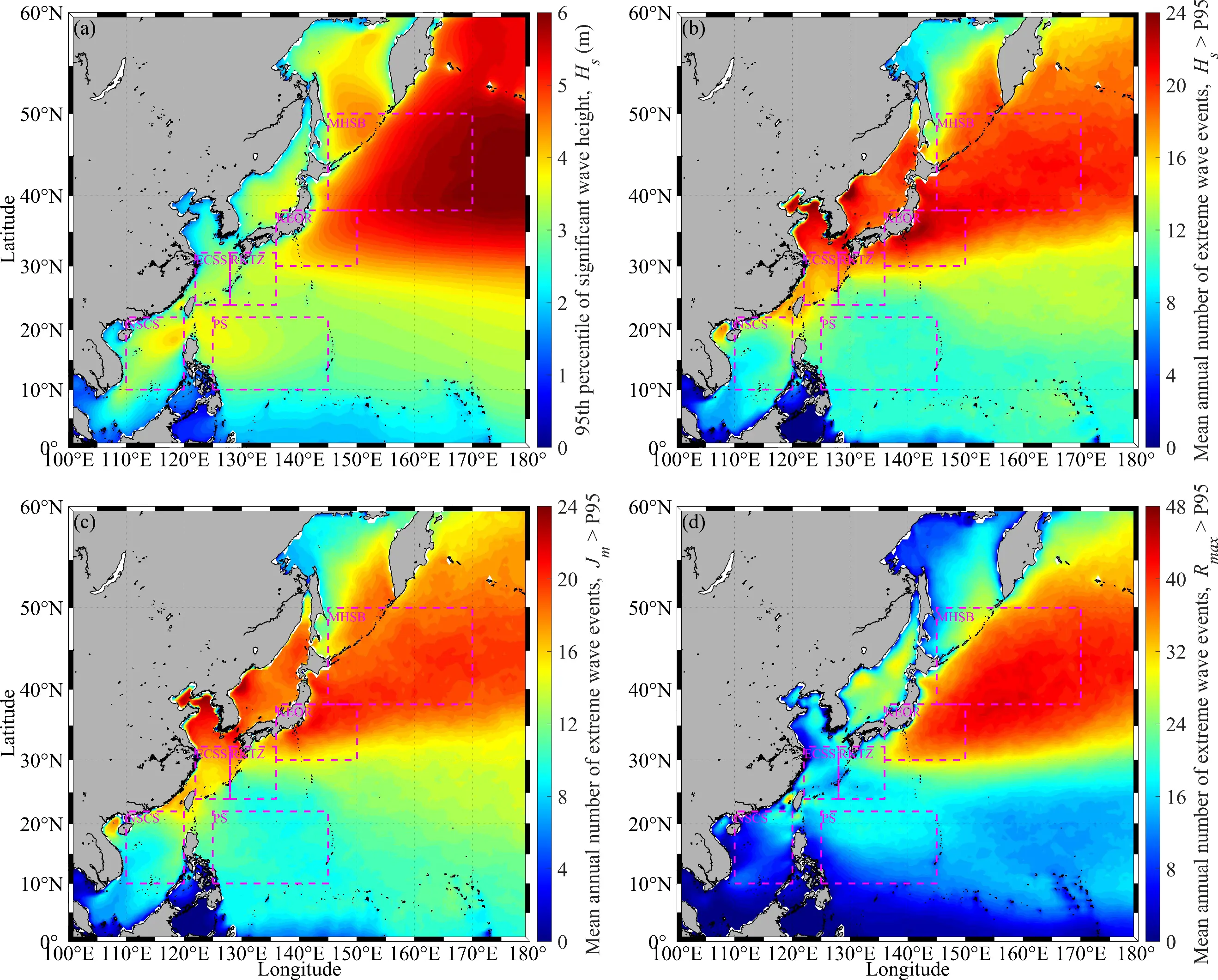
Figure 10. Extreme-load proxies: (a) local P95(Hs); annual declustered exceedance counts for (b) Hs > P95local, (c) Jm > P95local, and (d) Rmax > P95local. Events use a 24 h declustering interval and Hs ≥ 2 m.
The use of a concurrent Hs ≥ 2 m condition in the extreme event definition is important for engineering interpretation. As shown in the Hs–Tm matrices in Figure 5, a large fraction of background sea states in marginal and subtropical regions lies around Hs ≈ 1–2 m and relatively low wave-power contours. Without a minimum-wave-height condition, local-percentile exceedances or high Rmax ratios under weak sea states could inflate event counts that are not relevant to structural loading or WEC survivability. The Hs ≥ 2 m filter, therefore, focuses risk diagnostics on sea states more relevant to structural loading while still allowing local thresholds to account for regional differences in wave climate.
The three event-frequency metrics diagnose different dimensions of risk. EHs95 primarily reflects the frequency of high-wave-load conditions, EJm95 reflects the frequency of high-energy sea states relevant to both resource yield and load exposure, and ER95 reflects the relative occurrence of high individual-wave amplification conditions. Their spatial similarities confirm that the storm-belt and western-boundary transition regions are risk-prone environments. Their differences show that no single metric can fully describe operational risk. In particular, regions with moderate P95(Hs) may still experience frequent high-power events if wave periods are long, whereas regions with high Rmax event frequency may indicate enhanced amplification of individual waves even when mean resource levels are not locally maximal. From a resource-quality perspective, Figure 10 strengthens the interpretation developed from Figure 1, Figure 2, Figure 3, Figure 4, Figure 5, Figure 6, Figure 7, Figure 8 and Figure 9. The MHSB and KEOR are not only high-resource and high-availability regions; they also show elevated frequencies of high-wave, high-power, and amplification-risk events. This indicates that their resource advantage is coupled with greater exposure to operational and survivability constraints. Conversely, subtropical and marginal-sea regions generally have lower event frequencies but also lower mean resource and availability. The Northwest Pacific therefore exhibits clear resource–risk coupling in the storm-belt regime and a resource–risk trade-off across the basin.
Physically, the risk maxima are consistent with the dominant role of winter extratropical storms and storm-wave propagation east of Japan. The largest P95(Hs) and ER95 values occur where strong winds, long fetch, and open-ocean propagation can generate both large wave heights and more variable individual-wave conditions. The elevated EHs95 and EJm95 values along the western boundary and shelf-transition zones likely reflect the combined influence of winter monsoon forcing, storm tracks, tropical-cyclone remnants, topographic effects, and open-ocean exposure. This agrees with earlier wave-climate and wave-energy studies showing that the western North Pacific and adjacent marginal seas are shaped by both extratropical and tropical storm systems, as well as monsoonal variability.
The resource–risk phase-space diagrams provide a direct synthesis of the spatial patterns shown in Figure 1 and Figure 10. When long-term mean wave power is compared with the annual number of declustered Hs > P95local events, the analyzed grid cells form a broad but structured distribution (Figure 11a). The median-based thresholds divide the domain at approximately Jm ≈ 18 kW·m−1 and EHs95 ≈ 12–13 events yr−1. Most high-resource grid cells, particularly those with Jm > 30 kW·m−1, fall within the high-resource–high-risk quadrant, with EHs95 commonly around 16–22 events yr−1. In contrast, the high-resource–low-risk quadrant is sparsely populated. This indicates that, for the Hs-based extreme-load metric, a large mean wave power is rarely achieved without an elevated frequency of high-wave events.
The subregional mean markers clarify this basin-scale structure. The MHSB occupies the most energetic position, with a mean Jm of approximately 40–45 kW·m−1 and EHs95 of 20 events yr−1, placing it clearly in the high-resource–high-risk quadrant. The KEOR also falls within this quadrant, with a lower but still elevated mean resource of 25–27 kW·m−1 and a similar high-wave event frequency near 20 events yr−1. These two regions are therefore not only high-power regimes but also high-load-exposure regimes. This interpretation is consistent with their storm-belt and open-ocean exposure, as identified in Figure 1, Figure 2, Figure 3 and Figure 4, and their high winter availability, as shown in Figure 8.
The lower-resource subregions show more varied risk behavior. The NSCS and PS have mean Jm values below or near the resource threshold, approximately 10–17 kW·m−1, and EHs95 values around 10–11 events yr−1, placing them within or near the low-resource–low-risk sector. The ECSS, however, has relatively low mean wave power, approximately 12 kW·m−1, but a higher EHs95 of 17 events yr−1, placing it in the low-resource–high-risk quadrant. This is an important distinction: a region can have modest mean wave power but still experience frequent local high-wave exceedance events. For the ECSS, this likely reflects episodic monsoon, typhoon, and shelf-edge wave events superimposed on a generally moderate background wave climate. The RKTZ lies close to the median thresholds, with mean Jm around 17 kW·m−1 and EHs95 around 14–15 events yr−1, consistent with its transition-zone character between shelf, subtropical open-ocean, and Kuroshio-influenced wave regimes.
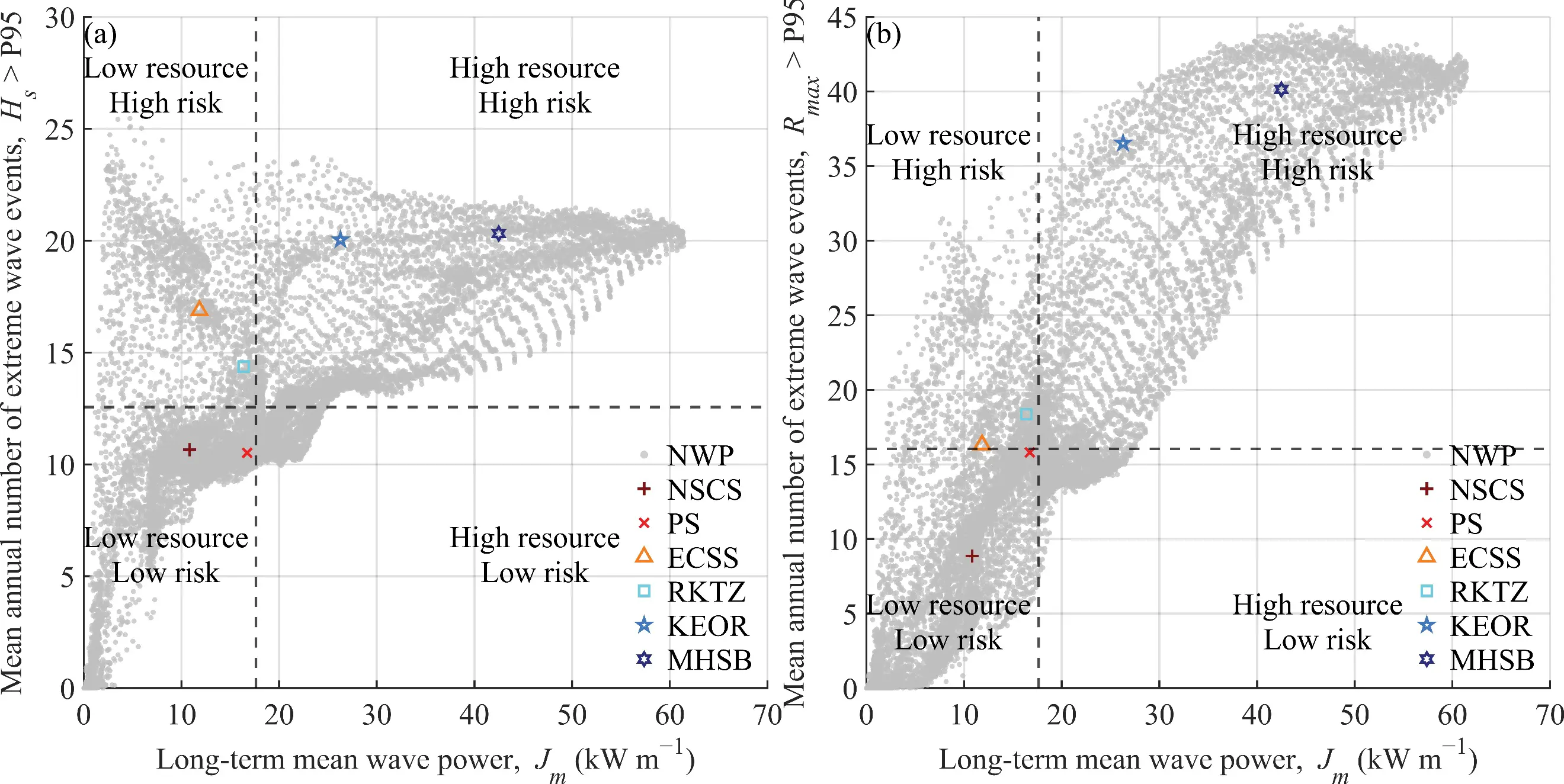
Figure 11. Resource–risk phase spaces relating mean Jm to annual declustered exceedance counts for (a) Hs > P95local and (b) Rmax > P95local. Grey points represent grid cells, symbols show subregional means, and dashed lines denote population medians.
The Rmax-based phase space shows a stronger coupling between resource intensity and wave-amplification risk (Figure 11b). The median thresholds are Jm ≈ 18 kW·m−1 and ER95 ≈ 16 events yr−1. Unlike the Hs-based diagram, the grid-cell distribution shows a clearer increase in ER95 with increasing Jm. High-resource grid cells with Jm > 30 kW·m−1 almost entirely occupy the high-resource–high-risk quadrant, with ER95 commonly exceeding 25–40 events yr−1. The high-resource–low-risk quadrant is nearly empty. This indicates that the energetic open-ocean regime is not only associated with more frequent high-wave events but also with more frequent high-amplification conditions, as represented by the ERA5 Rmax proxy. The subregional positions reinforce this result. The MHSB has the highest mean wave power and the highest Rmax-based event frequency, with ER95 close to 40 events yr−1. The KEOR is also strongly elevated, with ER95 around 36–37 events yr−1. These values are much higher than their corresponding EHs95 values in Figure 11a, suggesting that the amplification-risk proxy responds more strongly to the storm-generated open-ocean regime than the high-wave exceedance metric alone. The RKTZ and ECSS lie near or slightly above the risk threshold, whereas the PS lies close to the resource threshold but remains comparatively lower in ER95. The NSCS is clearly positioned within the low-resource–low-risk sector, with ER95 below 10 events yr−1.
The two phase-space diagrams, therefore, provide complementary perspectives. The Hs-based risk metric highlights high-wave load exposure and identifies both storm-belt high-resource regions and some marginal-sea low-resource but high-risk regions. The Rmax-based metric emphasizes amplification-related risk and shows a tighter association with high-resource open-ocean conditions. This difference is physically meaningful. High Hs events can arise from local exceedances in marginal or shelf seas, whereas high-Rmax events are more concentrated in storm-wave environments where energetic seas, spectral variability, and wave-system interactions are more frequent. Because Hmax in ERA5 is a statistical estimate rather than an observed individual-wave record, the Rmax results should be interpreted as relative amplification-risk diagnostics rather than observed rogue-wave frequencies. Nevertheless, the contrast between the two diagrams is useful for resource-quality assessment because it shows that different risk proxies do not identify exactly the same regions. Therefore, the evaluation of wave-energy resources requires more than ranking regions by mean Jm. A high-resource region may provide large theoretical energy potential but also impose greater operational and survivability constraints, whereas a moderate-resource region may be more attractive if risk exposure and temporal variability are lower.
3.4. Wind-Sea/Swell Source Proxies and Resource-Quality Contrasts
The spatial distribution of the swell-contribution proxy, Cswell, reveals a clear source-structure contrast that underlies the resource and risk patterns discussed above (Figure 12). Since Cwind = 1 − Cswell, regions with low Cswell have a stronger relative wind-sea contribution, whereas high Cswell indicates a more swell-dominated wave climate. Figure 12a–d therefore provides the physical background for interpreting why some high-power regions are more variable and risk-prone, whereas some moderate-power regions exhibit more stable resource characteristics.
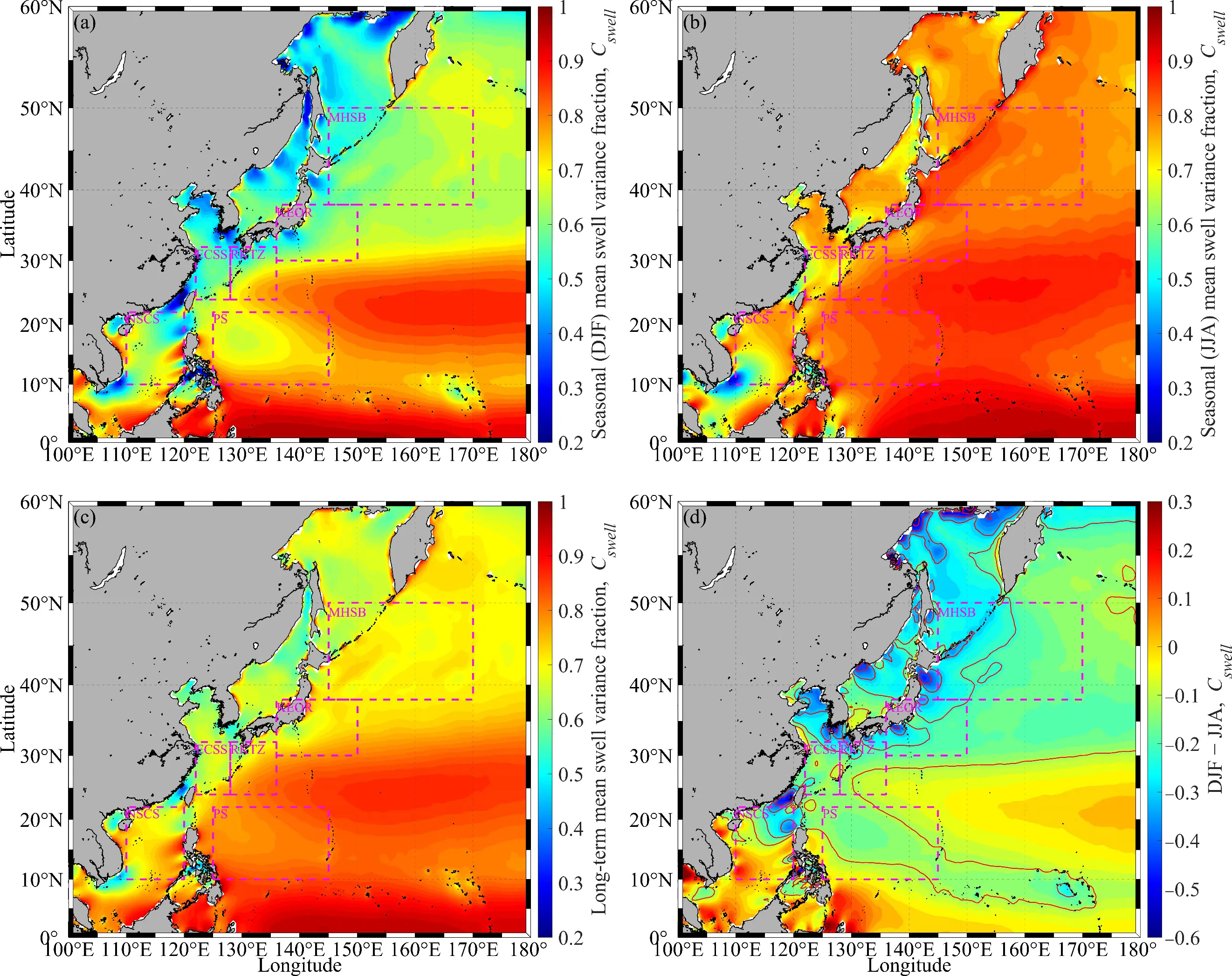
Figure 12. Seasonal and long-term distributions of Cswell: (a) DJF mean, (b) JJA mean, (c) long-term mean, and (d) DJF–JJA difference. Red contours in (d) identify Cswell,DJF < Cswell,JJA. Magenta dashed boxes denote the six diagnostic subregions.
During DJF, the Northwest Pacific shows strong meridional and coastal gradients in Cswell (Figure 12a). The subtropical open Pacific, especially the southern and eastern parts of the PS and the low-latitude western Pacific, is strongly swell dominated, with Cswell commonly exceeding 0.8 and locally approaching 0.9–1.0. In contrast, lower Cswell values occur along the East Asian margin, around Japan, within the Japan Sea–Okhotsk sector, across the ECSS–RKTZ transition, and in parts of the KEOR. In these regions, Cswell frequently decreases to approximately 0.4–0.7 and is locally still lower near semi-enclosed or coastal seas. This indicates a much larger winter wind-sea contribution. The pattern is consistent with the winter dominance of wave power in Figure 2 and Figure 3: the high-energy winter resource is not purely a swell resource but is strongly associated with locally or regionally generated wind seas driven by winter monsoon and extratropical storm activity.
The JJA distribution is substantially more swell dominated over most of the basin (Figure 12b). Large areas of the open Northwest Pacific, including the PS, RKTZ, KEOR, and much of the MHSB, show Cswell > 0.8, with broad subtropical and mid-latitude regions approaching 0.9. This seasonal increase in Cswell coincides with the weakening of the winter storm-wave regime and the reduction of Jm and A10 in summer (Figure 2, Figure 3, Figure 8 and Figure 9). Thus, summer wave conditions are generally more swell dominated but less energetic. Exceptions remain in some marginal or semi-enclosed seas, where Cswell can remain near 0.4–0.6, reflecting local wind-sea generation, coastal geometry, and restricted fetch.
The long-term mean Cswell integrates these seasonal contrasts and highlights the dominant wave-system structure of each subregion (Figure 12c). The PS is the most clearly swell-dominated region among the six diagnostic boxes, with long-term Cswell mostly above 0.8. This agrees with its moderate but persistent resource behavior in the preceding sections. The RKTZ and KEOR show intermediate-to-high Cswell, generally around 0.65–0.85, reflecting their transitional character between open-ocean swell influence and storm-generated western-boundary wave systems. The MHSB has a relatively high long-term Cswell in its eastern open-ocean part but lower values near its western and northern margins, indicating that the storm-belt resource is a mixed regime rather than a purely swell-dominated one. The ECSS and NSCS exhibit stronger spatial heterogeneity, with shelf and coastal waters generally showing lower Cswell than exposed open-ocean regions. This heterogeneity is consistent with the stronger influence of monsoon winds, local fetch, and shelf–coastal effects in marginal seas.
The DJF–JJA difference map further clarifies the seasonal source transition (Figure 12d). Red contours mark the boundary of areas where Cswell,DJF < Cswell,JJA. North of this boundary, especially around Japan, the KEOR, the MHSB, and high-latitude marginal seas, the difference is mostly negative, commonly around −0.1 to −0.3 and locally lower. This indicates that the winter wind-sea contribution is stronger. This region generally coincides with large winter Jm, high-percentile wave power, A10, and risk-event frequencies. The source-composition contrast, therefore, supports the interpretation that the high-power winter regime east of Japan is storm generated and wind-sea enhanced. South of approximately 30° N, the difference becomes weakly positive over several subtropical and low-latitude open-ocean areas, with Cswell,DJF − Cswell,JJA locally reaching approximately 0.1–0.2. This suggests that DJF conditions in these regions can be more swell dominated than summer conditions. A plausible explanation is that winter swell generated by mid-latitude storms propagates into lower-latitude regions, whereas summer conditions may include more local wind sea or tropical-weather influence. Similar distinctions between locally forced wind sea and remotely generated swell have been emphasized in global wind-sea/swell climatology and spectral-partitioning studies [16,17,18]. Thus, the seasonal source transition is not simply a local wind-speed signal; it reflects basin-scale wave-generation and propagation pathways.
The monthly cycles of Cswell provide a subregional view of the seasonal source transitions identified in Figure 12. Overall, all six regions are swell influenced throughout the year, with monthly median Cswell mostly above 0.6. However, the amplitude, phase, and persistence of the swell contribution differ substantially among subregions. These differences help explain why regions with comparable wave-power availability can have different resource-quality characteristics.
The PS is the most persistently swell-dominated region (Figure 13b). Its monthly median Cswell remains high throughout the year, increasing from approximately 0.72 in January to a maximum of approximately 0.88 in May and remaining mostly between 0.83 and 0.86 from June to October before decreasing to approximately 0.76 in December. This high and relatively stable swell contribution is consistent with the PS being an open-ocean tropical region exposed to remote swell propagation. Compared with its wave-power cycle in Figure 3 and availability cycle in Figure 9, the PS shows a clear contrast: Jm and A10 decrease strongly in late spring and early summer, but Cswell remains high. This indicates that the low-resource season in the PS is not caused by a loss of swell dominance but by a reduction in wave height and energy level. The relatively steady wave climate of the PS is consistent with its geographical position. Although the region is less directly exposed to the core of the mid-latitude winter storm track, it receives remotely generated, long-period swell from distant generation regions. Long-distance propagation separates the swell field from more locally forced wind-sea variability, contributing to a smoother wave climate than that of the directly forced KEOR and MHSB.
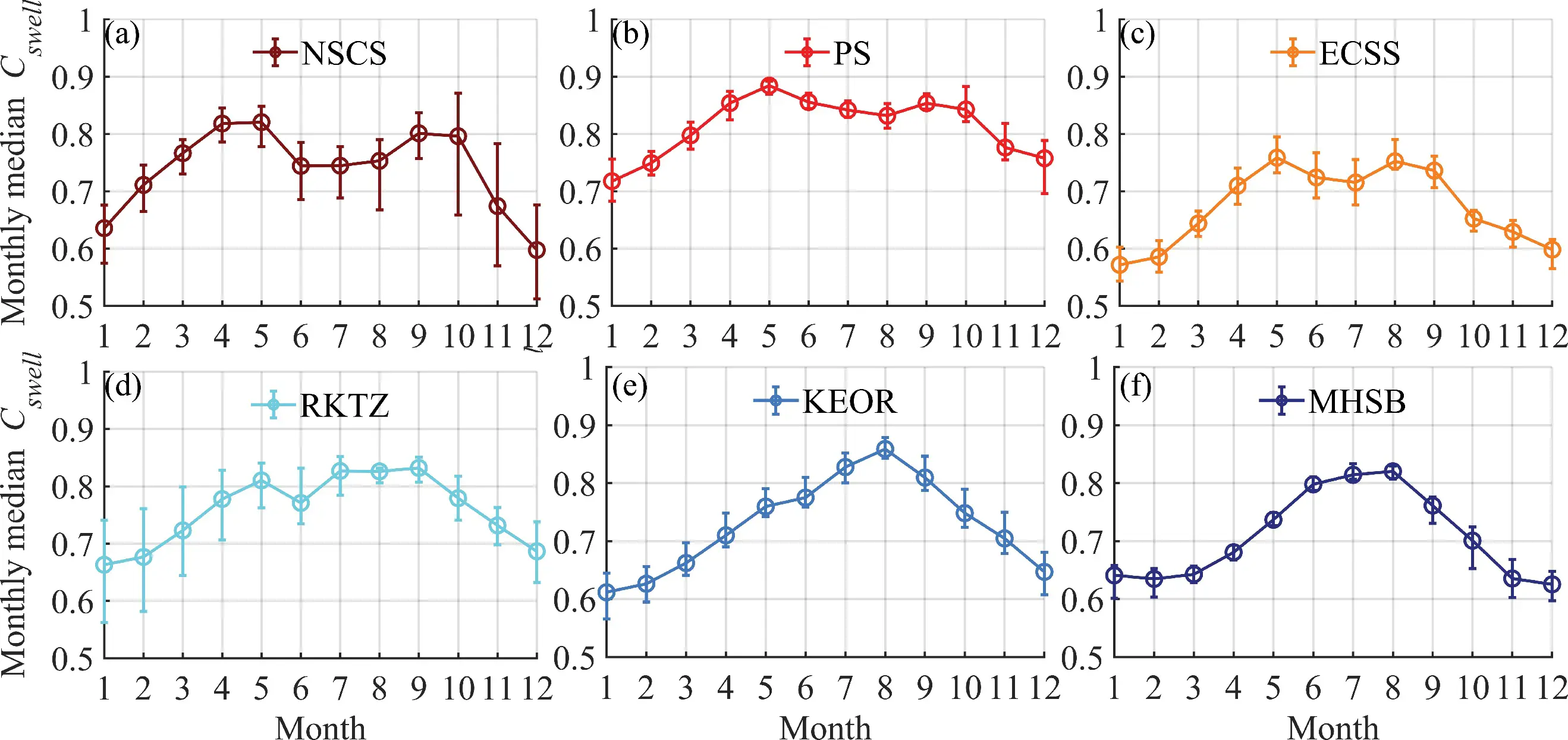
Figure 13. Monthly evolution of Cswell in (a) NSCS, (b) PS, (c) ECSS, (d) RKTZ, (e) KEOR, and (f) MHSB. Circles denote monthly medians, and vertical bars show the interquartile range across grid cells.
The KEOR and MHSB show stronger seasonal source transitions. In the KEOR, monthly median Cswell is 0.61–0.66 in winter, increases gradually through spring, and reaches a maximum of 0.85–0.87 in August before decreasing again toward winter. The MHSB behaves similarly: Cswell is approximately 0.63–0.65 during December–February, increases to 0.80–0.82 during June–August, and then decreases after September. Since Cwind = 1 − Cswell, these curves imply that the wind-sea contribution in the KEOR and MHSB is much larger in winter than in summer. For example, winter Cwind is 0.35–0.40 in the KEOR and MHSB, whereas summer Cwind decreases to 0.15–0.20. This seasonal reversal is directly consistent with Figure 2, Figure 3, Figure 8 and Figure 9: periods of highest wave power and availability in the KEOR and MHSB coincide with reduced Cswell, indicating stronger wind-sea or mixed-sea influence during the energetic winter season. The RKTZ also exhibits a clear seasonal increase in swell contribution from winter to summer. Monthly median Cswell rises from approximately 0.66–0.68 in January–February to 0.80–0.83 between July and September, before decreasing to 0.68 in December. This pattern supports the interpretation of the RKTZ as a transition region. In Figure 3d, the RKTZ shows enhanced wave power during late summer and autumn rather than a purely winter-dominant cycle. In Figure 13d, the same period corresponds to relatively high Cswell, suggesting that part of the late-summer to autumn resource in the RKTZ is supported by open-ocean swell or remotely generated wave systems rather than solely by local winter wind sea. The wider interquartile ranges in several months also indicate strong spatial heterogeneity within the region, consistent with its position between the East China Sea shelf, the Ryukyu island chain, and the open Pacific.
The ECSS has a lower swell contribution than the PS, RKTZ, KEOR, and summer MHSB, yet its seasonal cycle remains evident (Figure 13c). Monthly median Cswell is approximately 0.57–0.60 in winter, increases to 0.70–0.76 from April to August, and then decreases again toward 0.60 in December. Thus, winter in the ECSS is relatively more wind-sea influenced, consistent with East Asian winter-monsoon forcing and shelf-sea wave generation. During spring and summer, the increase in Cswell indicates a larger relative contribution from swell or longer-period incoming waves. This behavior helps explain why the ECSS has modest wave-power intensity but a relatively complex seasonal structure in Figure 3 and Figure 9. The NSCS exhibits a distinct marginal-sea pattern (Figure 13a). Median Cswell is approximately 0.64 in January, increases to 0.80–0.82 in April–May, remains near 0.74–0.80 from June to October, and decreases to 0.60 in December. The lowest Cswell values occur during late autumn and winter, when Jm and A10 increase sharply in Figure 3 and Figure 9. This indicates that the winter wave-energy enhancement in the NSCS is associated with a larger local wind-sea contribution, most likely related to the East Asian winter monsoon. In contrast, spring and summer conditions are more swell dominated but less energetic. The NSCS, therefore, illustrates a common marginal-sea resource pattern: the most energetic months are not necessarily the most swell dominated.
Across the six regions, Figure 13 suggests an important phase relationship between source composition and resource magnitude. In the KEOR, MHSB, ECSS, and NSCS, Cswell tends to be lower during months of higher wave power or higher A10 and higher during the lower-energy summer months. This inverse relationship indicates that the strongest wave-energy conditions are often associated with enhanced wind-sea or mixed-sea contribution. Conversely, more swell-dominated periods tend to be smoother but less energetic. The PS is a partial exception because it remains swell dominated throughout the year, even though its resource magnitude varies seasonally. This makes the PS a useful contrast to the storm-belt regions: it is not the strongest resource region, but it has a consistently high swell fraction. This source–seasonality relationship is central to the resource-quality interpretation. The storm-belt high-power regime identified in Figure 1, Figure 2, Figure 3, Figure 4, Figure 5 and Figure 6 is not simply a high-swell regime; it is a winter wind-sea-enhanced or mixed regime. This helps explain why the KEOR and MHSB combine high resource intensity with strong seasonality and elevated risk exposure. In contrast, the PS and parts of the RKTZ have more persistent swell dominance, which is consistent with their more moderate but potentially higher-quality resource characteristics. These results agree with established wave-climate understanding that wind seas are more closely tied to local wind forcing and storm variability, whereas swells are generated remotely and can provide broader, smoother propagation signals [16,17,18].
The class-based comparison provides evidence consistent with a relationship between resource quality and wave-source composition. Rather than examining Cswell geographically, this analysis groups grid cells by resource intensity, stability, and risk exposure, then compares their annual mean swell contributions. The resource classes show a clear contrast (Figure 14a). High-resource grid cells have a lower median Cswell, approximately 0.71, whereas intermediate-resource grid cells have a higher median value of 0.82. In other words, the high-resource class has an implied wind-sea contribution of 0.29, compared with 0.18 in the intermediate-resource class. This difference is consistent with the spatial patterns in Figure 1, Figure 2, Figure 3, Figure 4, Figure 5 and Figure 6 and the seasonal source analysis in Figure 12 and Figure 13: the strongest wave-power resources in the Northwest Pacific are not primarily associated with purely swell-dominated conditions but with wind-sea-enhanced or mixed regimes generated by winter storms and strong regional wind forcing. The relatively narrow interquartile range of the high-resource group also suggests that this lower-swell, higher-wind-sea signature is a systematic feature of the high-power regime rather than a local anomaly.
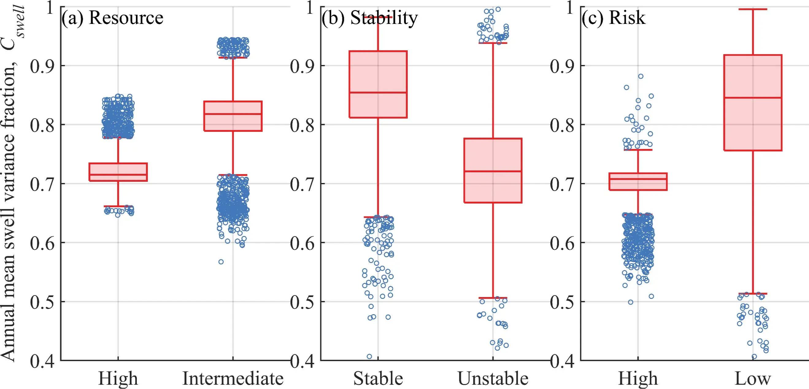
Figure 14. Annual mean Cswell by (a) resource, (b) stability, and (c) risk class. Boxes show interquartile ranges and medians; whiskers denote non-outlier ranges, and points represent individual grid cells. Classes are defined from percentile ranges of Jm, CVm, and EHs95.
The stability classes reveal the opposite tendency (Figure 14b). Stable grid cells show substantially higher Cswell, with a median near 0.85, whereas unstable grid cells have a lower median of approximately 0.72. This implies that stable resources are more swell dominated, whereas unstable resources have a stronger wind-sea component. The result agrees with the physical expectation that swell-dominated wave systems, generated remotely and propagated over long distances, tend to be smoother and less tightly coupled to local storm variability than wind seas [16,17,18]. It also helps explain why some moderate-power regions in the PS and parts of the RKTZ can display better temporal persistence than the storm-belt high-power regions. Their resource magnitude is lower, but their higher swell contribution is associated with reduced monthly and seasonal variability. The risk classes provide a complementary indication of the same source-dependent structure (Figure 14c). High-risk grid cells have a median Cswell of approximately 0.70, whereas low-risk grid cells have a much higher median value near 0.84. The high-risk distribution is also concentrated around relatively low Cswell, indicating that elevated extreme-event exposure is strongly associated with wind-sea or mixed-sea conditions. This is consistent with the risk maps and resource–risk phase-space diagrams in Figure 10 and Figure 11, where the MHSB and KEOR combine high wave power with frequent high-wave, high-power, and wave-amplification events.
These results extend the interpretation beyond a purely statistical trade-off. The intensity–persistence–risk contrast is not only a consequence of the selected thresholds or screening metrics; it is also associated with the inferred source structure of the wave field. Storm-generated wind seas and mixed sea states produce high energy but are accompanied by stronger variability and risk, whereas swell-dominated regimes tend to provide more moderate but steadier resources. Cswell therefore provides an interpretable proxy for relating resource magnitude, stability, and risk exposure.
3.5. Integrated Technical Pre-Screening of Wave-Energy Priority Zones
The composite pre-screening score integrates resource intensity, availability, stability, water-depth suitability, and risk-proxy information discussed in the preceding sections (Figure 15). The resulting pattern differs substantially from the mean wave-power distribution in Figure 1, indicating that high mean wave power alone does not identify the most favorable wave-energy resource zones. The score ranges from approximately 0.25 to 0.65 across the study domain. The highest scores occur not in the storm-belt high-power core east of Japan but in several transition and moderate-resource areas where resource intensity, availability, stability, risk exposure, and water-depth suitability are jointly more favorable. A notable feature of Figure 15a is the reduced score within much of the MHSB and KEOR despite their high mean and upper-tail wave power. These regions have high resource and availability scores, but they are penalized by strong seasonality, elevated extreme-event frequencies, elevated amplification-risk proxy values, and less favorable water-depth suitability in parts of the offshore domain. Within the MHSB, many grid cells remain in the moderate score range of approximately 0.35–0.45, which is considerably lower than would be suggested by resource intensity alone. This result is consistent with the preceding analysis: the storm-belt regime is energetic and highly available in winter, but it is also strongly seasonal and risk-prone.
By contrast, relatively high scores occur in several moderate-resource transition zones. Elevated scores, generally ranging from 0.50 to 0.60 and locally approaching 0.65, occur along parts of the western boundary transition region, around the Ryukyu–Taiwan sector, the East China Sea shelf break, the northern South China Sea, and portions of the subtropical open Northwest Pacific. These regions do not have the largest mean Jm, but they combine moderate resource intensity with more favorable stability or risk characteristics. This supports the central resource-quality interpretation developed in this study: regions with moderate wave power can become more favorable when persistence, risk exposure, and water-depth suitability are considered jointly. The low-latitude and subtropical open-ocean sectors also exhibit relatively high composite scores in some areas. This is likely related to their larger swell contribution, lower seasonal variability, and reduced extreme-load exposure compared with the storm-belt core. However, many of these high-score open-ocean cells are far from land and infrastructure. Because distance to shore, port access, shipping constraints, and marine spatial planning were not included in the screening index, these remote high-score areas should be regarded only as zones with favorable physical resource-quality characteristics, not as deployment-ready sites.
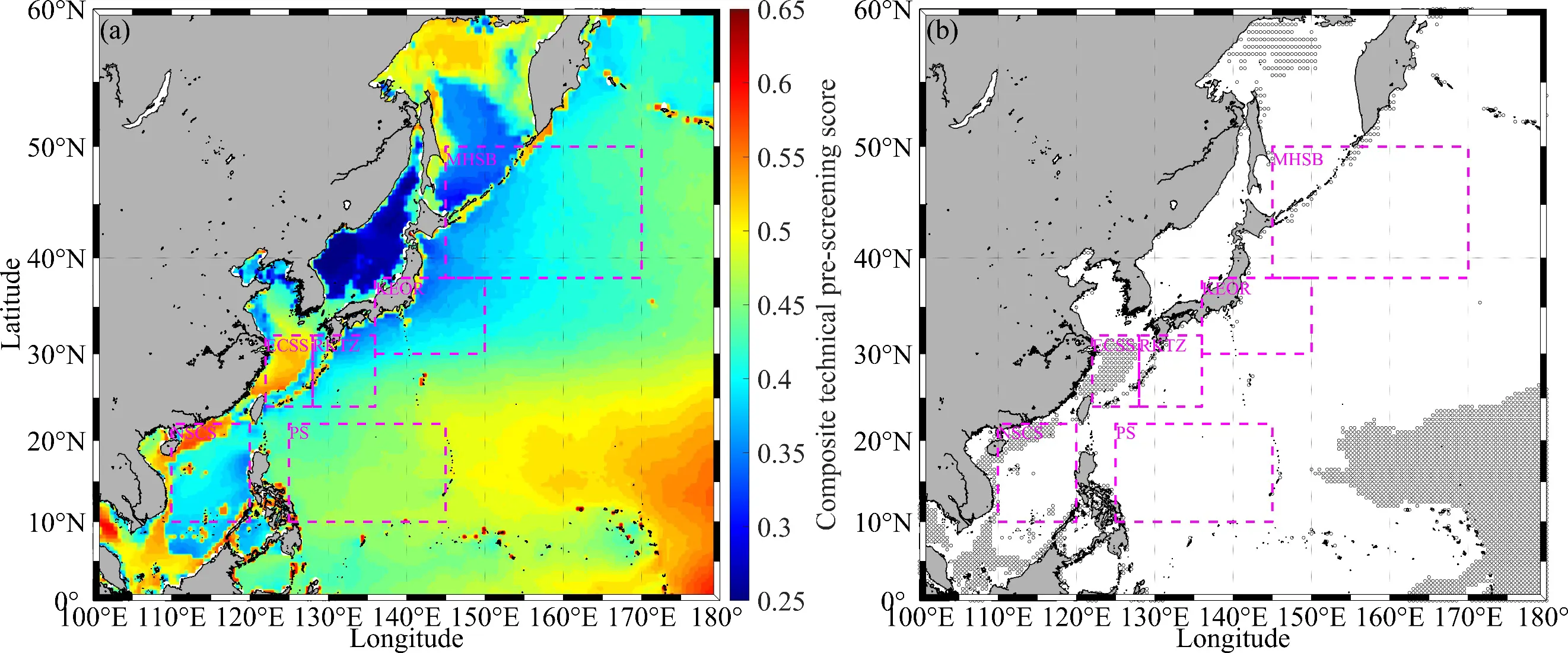
Figure 15. Integrated technical pre-screening of wave-energy priority zones: (a) composite score integrating resource intensity, availability, stability, water-depth suitability, extreme-load safety, and amplification-risk safety; and (b) top 20% priority candidate grid cells. Magenta dashed boxes denote the six diagnostic subregions.
The map of the top 20% candidate grid cells in Figure 15b further emphasizes that priority cells are spatially fragmented rather than concentrated within a single high-power region. Priority grid cells occur in several separated sectors, including parts of the western-boundary transition zone, shelf–open-ocean margins, and remote open-ocean regions. In contrast, the central MHSB and KEOR are not dominant among the top 20% of grid cells, even though they dominate the wave-power maps. This indicates that the screening procedure shifts the ranking from maximum resource intensity toward balanced resource quality. This further supports the need to distinguish between resource abundance and resource quality. The highest-energy region may remain valuable, but it is not automatically the most favorable region for detailed development or deployment assessment. Figure 15 should therefore be interpreted as a basin-scale technical pre-screening output rather than a final siting decision. The index does not include distance to shore, transmission costs, port proximity, marine protected areas, shipping lanes, fisheries, seabed constraints, device-specific power matrices, mooring design, or high-resolution nearshore wave transformation. These factors can substantially alter final site feasibility. Therefore, the top 20% areas should be understood as zones where high-resolution wave modeling, WEC-specific performance assessment, and engineering-economic screening are warranted. This interpretation is consistent with wave-energy resource-assessment guidance, which treats basin- or regional-scale resource characterization as an early stage before detailed site design and validation [10,11,38].
4. Conclusions
Using 45 years of six-hourly ERA5 reanalysis data, this study examined wave-energy resources across the Northwest Pacific by jointly considering wave-power intensity, temporal variability, availability, persistence, extreme-event exposure, and wind-sea/swell composition. The principal conclusions are summarized below.
Key findings:
-
-
The regions with the greatest theoretical wave-power intensity do not necessarily provide the highest practical resource quality. The mid- to high-latitude storm belt and the Kuroshio Extension contain the largest long-term mean, winter, and upper-tail wave-power resources, but their advantages are offset by strong seasonal concentration, reduced summer availability, and elevated extreme-event exposure. This spatial mismatch between maximum energy intensity and integrated resource quality is the central finding of the study.
-
-
Temporal variability fundamentally changes the interpretation of regional wave-energy potential. In the mid- to high-latitude storm belt and the Kuroshio Extension, the monthly coefficient of variation is generally approximately 0.5–0.7, while the seasonal variability index commonly exceeds 0.7. In contrast, parts of the Philippine Sea and the Ryukyu–Kuroshio transition zone exhibit weaker monthly and seasonal variability. Because strong variability concentrates energy production and structural loading within limited seasons, it represents a potential operational and cost penalty in the most energetic regions.
-
-
High wave-power intensity is strongly coupled with elevated risk exposure. Most high-resource grid cells also experience frequent high-wave, high-power, and wave-amplification events, whereas high-resource but low-risk conditions are comparatively rare. The energetic storm-belt resource should therefore be regarded as a high-power–high-risk regime rather than simply as the most favorable resource zone.
-
-
Wave-system composition provides a physical explanation for the contrast between resource intensity and resource quality. Stable and low-risk grid cells have median swell-contribution indices of approximately 0.85 and 0.84, respectively, compared with approximately 0.72 and 0.70 for unstable and high-risk grid cells. The highest-energy regions are more strongly influenced by winter wind sea and mixed sea states, whereas more persistent and lower-risk resources are generally associated with swell-dominated conditions.
-
-
Integrating intensity, availability, variability, water depth, and relative risk substantially changes the spatial ranking of potential wave-energy zones. The composite screening shifts priority away from the maximum-power storm-belt core toward several moderate-resource transition areas, including parts of the Philippine Sea, the Ryukyu–Kuroshio transition zone, the East China Sea shelf break, and the northern South China Sea. These regions do not maximize theoretical wave power, but they provide a more balanced combination of resource magnitude, persistence, and risk.
Limitations and precautions:
-
-
ERA5 is suitable for basin-scale climatological comparison and preliminary screening, but should not be used alone to define engineering design conditions. Severe ERA5 winds may underestimate extreme wave conditions when the significant wave height exceeds approximately 7.5 m. The upper-tail wave-power and extreme-event results should therefore be treated as relative regional indicators rather than as design wave heights, return-period conditions, or survivability limits.
-
-
The technical screening does not include device-specific power matrices, annual energy production, distance to shore, port and grid accessibility, environmental restrictions, mooring requirements, or high-resolution nearshore wave transformation. The identified priority zones should therefore be interpreted as candidates for further assessment rather than final deployment sites.
Future research:
-
-
Future studies should validate and refine the ERA5-based resource and risk patterns using buoy observations, satellite altimetry, and high-resolution wave hindcasts driven by bias-corrected atmospheric forcing, particularly in tropical-cyclone and severe extratropical-storm conditions.
-
-
The present resource-quality framework should be coupled with device-specific power and survivability characteristics and engineering-economic models. Component-resolved spectral data should also be used to quantify separate wind-sea and swell energy fluxes and to assess the effects of directional spreading, spectral bandwidth, crossing seas, and wave–current interaction.
Statement of the Use of Generative AI and AI-Assisted Technologies in the Writing Process
During the preparation of this manuscript, the authors used ChatGPT (OpenAI) in order to improve the language and readability of the manuscript. After using this tool, the authors reviewed and edited the content as needed and take full responsibility for the content of the published article.
Acknowledgments
The authors acknowledge the Copernicus Climate Change Service (C3S) Climate Data Store (CDS) for providing the ERA5 ocean-wave reanalysis data used in this study. The authors are responsible for the use and interpretation of the Copernicus Climate Change Service information presented herein. The authors also acknowledge Rich Pawlowicz for providing the M_Map mapping package for MATLAB [39], which was used for map visualization.
Author Contributions
Conceptualization, X.C.; Methodology, X.C.; Formal Analysis, X.C. and Z.Z.; Investigation, X.C.; Resources, Z.Z.; Data Curation, Z.Z.; Writing—Original Draft Preparation, X.C.; Writing—Review & Editing, Z.Z., D.X., C.J. and W.C.; Visualization, X.C.; Supervision, D.X., C.J. and W.C.; Funding Acquisition, Z.Z. and D.X.
Ethics Statement
Not applicable.
Informed Consent Statement
Not applicable.
Data Availability Statement
The data that support the main findings of this study are available from the corresponding author upon reasonable request.
Funding
This research work was funded by the National Natural Science Foundation of China (grant numbers 52401340, U2443219, and 52179076) and the Tianjin Science and Technology Program (grant number 25ZXZSSS00840).
Declaration of Competing Interest
The authors declare that they have no known competing financial interests that could have appeared to influence the work reported in this paper.
References
- Drew B, Plummer AR, Sahinkaya MN. A review of wave energy converter technology. Proc. Inst. Mech. Eng. Part A J. Power Energy 2009, 223, 887–902. DOI:10.1243/09576509JPE782 [Google Scholar]
- Falcão AFO. Wave energy utilization: A review of the technologies. Renew. Sustain. Energy Rev. 2010, 14, 899–918. DOI:10.1016/j.rser.2009.11.003 [Google Scholar]
- Cornett AM. A global wave energy resource assessment. In Proceedings of the 18th International Offshore and Polar Engineering Conference, Vancouver, BC, Canada, 6–11 July 2008; pp. 318–326. [Google Scholar]
- Mørk G, Barstow S, Kabuth A, Pontes MT. Assessing the global wave energy potential. In Proceedings of the ASME 2010 29th International Conference on Ocean, Offshore and Arctic Engineering, Shanghai, China, 6–11 June 2010; Volume 3, pp. 447–454. DOI:10.1115/OMAE2010-20473 [Google Scholar]
- Arinaga RA, Cheung KF. Atlas of global wave energy from 10 years of reanalysis and hindcast data. Renew. Energy 2012, 39, 49–64. DOI:10.1016/j.renene.2011.06.039 [Google Scholar]
- Gunn K, Stock-Williams C. Quantifying the global wave power resource. Renew. Energy 2012, 44, 296–304. DOI:10.1016/j.renene.2012.01.101 [Google Scholar]
- Reguero BG, Losada IJ, Méndez FJ. A global wave power resource and its seasonal, interannual and long-term variability. Appl. Energy 2015, 148, 366–380. DOI:10.1016/j.apenergy.2015.03.114 [Google Scholar]
- Reguero BG, Losada IJ, Méndez FJ. A recent increase in global wave power as a consequence of oceanic warming. Nat. Commun. 2019, 10, 205. DOI:10.1038/s41467-018-08066-0 [Google Scholar]
- Hemer MA, Fan Y, Mori N, Semedo A, Wang XL. Projected changes in wave climate from a multi-model ensemble. Nat. Clim. Chang. 2013, 3, 471–476. DOI:10.1038/nclimate1791 [Google Scholar]
- IEC TS 62600-101:2024; Marine Energy—Wave, Tidal and Other Water Current Converters—Part 101: Wave Energy Resource Assessment and Characterization. International Electrotechnical Commission: Geneva, Switzerland, 2024; 61p. Available online: https://webstore.iec.ch/en/publication/66062 (accessed on 16 June 2026).
- Pitt E. Assessment of Wave Energy Resource; European Marine Energy Centre: Orkney, UK, 2009; 42p. Available online: https://www.emec.org.uk/?wpfb_dl=34 (accessed on 16 June 2026).
- Mackay EBL, Bahaj AS, Challenor PG. Uncertainty in wave energy resource assessment. Part 1: Historic data. Renew. Energy 2010, 35, 1792–1808. DOI:10.1016/j.renene.2009.10.026 [Google Scholar]
- Mackay EBL, Bahaj AS, Challenor PG. Uncertainty in wave energy resource assessment. Part 2: Variability and predictability. Renew. Energy 2010, 35, 1809–1819. DOI:10.1016/j.renene.2009.10.027 [Google Scholar]
- Lavidas G, Blok K. Shifting wave energy perceptions: The case for wave energy converter feasibility at milder resources. Renew. Energy 2021, 170, 1143–1155. DOI:10.1016/j.renene.2021.02.041 [Google Scholar]
- Fairley I, Lewis M, Robertson B, Hemer M, Masters I, Horrillo-Caraballo J, et al. A classification system for global wave energy resources based on multivariate clustering. Appl. Energy 2020, 262, 114515. DOI:10.1016/ j.apenergy.2020.114515 [Google Scholar]
- Semedo A, Sušelj K, Rutgersson A, Sterl A. A global view on the wind sea and swell climate and variability from ERA-40. J. Clim. 2011, 24, 1461–1479. DOI:10.1175/2010JCLI3718.1 [Google Scholar]
- Hanson JL, Phillips OM. Automated analysis of ocean surface directional wave spectra. J. Atmos. Oceanic Technol. 2001, 18, 277–293. DOI:10.1175/1520-0426(2001)018<0277>2.0.CO;2 [Google Scholar]
- Portilla J, Ocampo-Torres FJ, Monbaliu J. Spectral partitioning and identification of wind sea and swell. J. Atmos. Oceanic Technol. 2009, 26, 107–122. DOI:10.1175/2008JTECHO609.1 [Google Scholar]
- Zheng CW, Zhuang H, Li X, Li XQ. Wind energy and wave energy resources assessment in the East China Sea and South China Sea. Sci. China Technol. Sci. 2012, 55, 163–173. DOI:10.1007/s11431-011-4646-z [Google Scholar]
- Zheng CW, Pan J, Li JX. Assessing the China Sea wind energy and wave energy resources from 1988 to 2009. Ocean Eng. 2013, 65, 39–48. DOI:10.1016/j.oceaneng.2013.03.006 [Google Scholar]
- Liang B, Fan F, Liu F, Gao S, Zuo H. 22-year wave energy hindcast for the China East Adjacent Seas. Renew. Energy 2014, 71, 200–207. DOI:10.1016/j.renene.2014.05.027 [Google Scholar]
- Wan Y, Zhang J, Meng J, Wang J. A wave energy resource assessment in the China’s seas based on multi-satellite merged radar altimeter data. Acta Oceanol. Sin. 2015, 34, 115–124. DOI:10.1007/s13131-015-0627-6 [Google Scholar]
- Lin Y, Dong S, Wang Z, Guedes Soares C. Wave energy assessment in the China adjacent seas on the basis of a 20-year SWAN simulation with unstructured grids. Renew. Energy 2019, 136, 275–295. DOI:10.1016/j.renene.2019.01.011 [Google Scholar]
- Shi X, Liang B, Du S, Shao Z, Li S. Wave energy assessment in the China East Adjacent Seas based on a 25-year wave-current interaction numerical simulation. Renew. Energy 2022, 199, 1381–1407. DOI:10.1016/j.renene.2022.09.094 [Google Scholar]
- Panfilova M, Ponce de León S, Orejarena-Rondón AF, Bettencourt JH, Aouf L, Restano M, et al. Wave energy assessment using SWIM radar and high-resolution altimeter data. Energy Convers. Manag. X 2026, 31, 101971. DOI:10.1016/j.ecmx.2026.101971 [Google Scholar]
- Orejarena-Rondón AF, Panfilova M, Ponce de León S, Restano M, Sabia R, Benveniste J. High-resolution mapping of wave energy resources in the Mediterranean Sea using satellite altimetry. Energy Rep. 2026, 15, 109133. DOI:10.1016/j.egyr.2026.109133 [Google Scholar]
- Hersbach H, Bell B, Berrisford P, Hirahara S, Horányi A, Muñoz‐Sabater J, et al. The ERA5 global reanalysis. Q. J. R. Meteorol. Soc. 2020, 146, 1999–2049. DOI:10.1002/qj.3803 [Google Scholar]
- Stopa JE, Cheung KF. Intercomparison of wind and wave data from the ECMWF Reanalysis Interim and the NCEP Climate Forecast System Reanalysis. Ocean Model. 2014, 75, 65–83. DOI:10.1016/j.ocemod.2013.12.006 [Google Scholar]
- Feng X, Chen X. Feasibility of ERA5 reanalysis wind dataset on wave simulation for the western inner-shelf of Yellow Sea. Ocean Eng. 2021, 236, 109413. DOI:10.1016/j.oceaneng.2021.109413 [Google Scholar]
- Shi H, Cao X, Li Q, Li D, Sun J, You Z, et al. Evaluating the accuracy of ERA5 wave reanalysis in the water around China. J. Ocean Univ. China 2021, 20, 1–9. DOI:10.1007/s11802-021-4496-7 [Google Scholar]
- Zhai R, Huang C, Yang W, Tang L, Zhang W. Applicability evaluation of ERA5 wind and wave reanalysis data in the South China Sea. J. Oceanol. Limnol. 2023, 41, 495–517. DOI:10.1007/s00343-022-2047-8 [Google Scholar]
- Elshinnawy AI, Menéndez M, Medina R. A parameterization for the correction of ERA5 severe winds for extreme ocean wave modelling. Ocean. Eng. 2024, 312, 119048. DOI:10.1016/j.oceaneng.2024.119048 [Google Scholar]
- European Centre for Medium-Range Weather Forecasts. Maximum Individual Wave Height. ECMWF Parameter Database, Parameter 140218. Available online: https://codes.ecmwf.int/grib/param-db/140218 (accessed on 16 June 2026).
- Coles S. An Introduction to Statistical Modeling of Extreme Values; Springer: London, UK, 2001. DOI:10.1007/978-1-4471-3675-0 [Google Scholar]
- Ferreira JA, Guedes Soares C. An application of the peaks over threshold method to predict extremes of significant wave height. J. Offshore Mech. Arct. Eng. 1998, 120, 165–176. DOI:10.1115/1.2829537 [Google Scholar]
- Fedele F, Brennan J, Ponce de León S, Dudley J, Dias F. Real world ocean rogue waves explained without the modulational instability. Sci. Rep. 2016, 6, 27715. DOI:10.1038/srep27715 [Google Scholar]
- Cavaleri L, Bertotti L, Torrisi L, Bitner-Gregersen E, Serio M, Onorato M. Rogue waves in crossing seas: The Louis Majesty accident. J. Geophys. Res. Oceans 2012, 117, C00J10. DOI:10.1029/2012JC007923 [Google Scholar]
- IEC TS 62600-100:2024; Marine Energy—Wave, Tidal and Other Water Current Converters—Part 100: Electricity Producing Wave Energy Converters—Power Performance Assessment. International Electrotechnical Commission: Geneva, Switzerland, 2024; 62p. Available online: https://webstore.iec.ch/en/publication/66061 (accessed on 16 June 2026).
- Pawlowicz R. M_Map: A Mapping Package for MATLAB, version 1.4o [Computer Software]. Available online: https://www.eoas.ubc.ca/~rich/map.html (accessed on 16 June 2026).