
Hybrid Mooring Design for a Pendulum-Based Wave Energy Converter
Hybrid Mooring Design for a Pendulum-Based Wave Energy Converter
Xiaoqiang Jiang 1,2 Chenyu Zhao 1 Hongda Shi 2 Lars Johanning 1,*
Received: 09 June 2026 Revised: 03 July 2026 Accepted: 16 July 2026 Published: 29 July 2026

© 2026 The authors. This is an open access article under the Creative Commons Attribution 4.0 International License (https://creativecommons.org/licenses/by/4.0/).
1. Introduction
Given the increasing scarcity of nearshore and coastline resources, researchers in WEC pay more attention to floating structures, which makes the study of mooring systems particularly important. The mooring system serves not only a station-keeping function, but also constitutes a key subsystem affecting survivability, operational reliability, and life-cycle cost. Moreover, compared with traditional offshore structures, WECs’ mooring systems often account for a larger proportion of the total cost [1,2]. The design of WEC mooring systems should strike a balance between energy acquisition and structural safety. Generally, good capture performance requires violent responses, which obviously differ from the traditional mooring design for ships and platforms in which the primary objective is stability [3,4].
In the past decades, substantial progress has been made in the development of mooring materials, configurations, and layouts. Although traditional catenaries are still widely adopted, taut, semi-taut, and hybrid lines employing synthetic fibre ropes such as nylon and polyester are being used more in WEC design and research [5,6]. Polyester ropes are widely used in offshore mooring systems because of their desirable tension-fatigue performance and resistance to corrosion, while nylon ropes can provide higher axial compliance and may further reduce dynamic mooring loads [7,8]. However, their nonlinear dynamic axial stiffness may lead to noticeable differences in the predicted platform motion, tension, and fatigue damage. On the other hand, novel concepts such as shared mooring systems have also attracted increasing attention in studies of WEC arrays [9,10,11]. With the development of mooring materials and configurations, analysis methods have evolved from quasi-static approaches to nonlinear methods, such as the lumped-mass method and the finite element method, which take inertia, drag forces, and geometric nonlinear effects into consideration [12,13].
In terms of the pendulum-based WECs (also known as rotating mass devices), Cordonnier et al. [14] introduced their series study on SEAREV, suggested that connecting the mooring lines close to the mean pitch rotation center can minimize mooring disturbance to output performance, and the SALM configuration has smaller extreme loads than the spread mooring. Sirigu et al. [15] improved the mooring system of ISWEC by adding a clump weight to reduce mooring load. Paduano et al. [16] analyzed the productivity effects of a 4-leg mooring system on the PeWEC and concluded that mooring analysis should be carefully analyzed for such a pitch-dependent WEC to avoid output overestimation. Cervelli et al. [17] evaluated the influence of multidirectional waves on PeWEC and stressed that the monodirectional approximation overestimates the performance. Xue et al. [18,19] tested ERWEC in several mooring layouts and wave directions, which reveals the fact that the buoy orientation and incident waves play important roles in its performance.
Generally, these works are mostly on vertical pendulum devices, while work on horizontal pendulums is rare. Furthermore, they focus mainly on local parameter analysis rather than on comprehensive design, although there is indeed extensive literature that elaborates on the relatively complete WEC mooring design process for other types. For instance, Depalo et al. [20] proposed an efficient approach for preliminary design of WEC mooring systems, which combined static analysis, frequency-domain quasi-static analysis, time-domain analysis, and code check under DNV rules. More recently, Zhao et al. [21] proposed a three-stage mooring design for the OE35 device, from initial concept development to design verification. However, the significant differences in the operating mechanisms between different WEC types often preclude the direct transfer of mooring design experience from one type to another. For example, a 3-leg spread mooring system has small effects on a buoy’s heave motion while significantly weakening its pitch response [22]. It is not a matter for a point absorber that captures wave power through heave motion, but it obviously affects the performance of devices relying on pitch response. Therefore, a comprehensive and systematic mooring design framework tailored for the pendulum-based WECs is necessary, and it is also required to strike a balance between safety and production.
In this study, one of the pendulum-based WECs [23,24] is selected, and a systematic mooring design is conducted. The remainder of this paper is structured as follows: Section 2 introduces the validation of the numerical model and provides a comprehensive flow of mooring design, from the initial environmental investigation to the safety check at a later stage. Section 3 presents the final design and discusses the results. Section 4 summarizes the main findings and contributions.
2. Model Validation and Mooring Design Methodology
The numerical model of the WEC is established and validated against experimental results. Then, a systematic mooring design is conducted based on that validated model, including the environmental investigation, step-by-step optimization of mooring parameters, and finally the safety code check.
2.1. WEC Concept
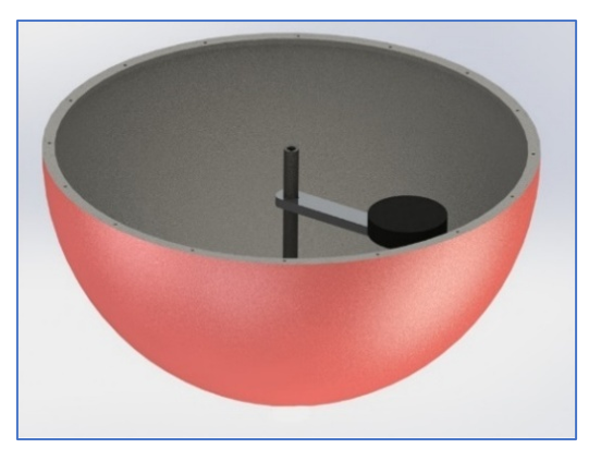
The concept of the selected pendulum-based WEC, or the rotating mass device on a vertical axis, is demonstrated in Figure 1. Its key components are the semi-sphere buoy and a vertical-axis pendulum encapsulated inside. When the buoy is riding on the wave, its multi-DOF motion leads to the response of the pendulum and the production of electricity.
2.2. Validation of Dynamic Simulation
A dynamic simulation for the moored pendulum-based WEC device was established using OrcaFlex [25], one of the industry benchmarks in mooring analysis. In this model, the hydrodynamics are simulated through linear wave theory, and the mooring dynamics are modelled by a nonlinear lumped-mass approach with a fully coupled strategy, which has comprehensive applications and good numerical stability.
The numerical model was validated by the experimental campaign, as shown in Figure 2. The key parameters of this physical model are listed in Table 1, and its pitch natural period is approximately 1.4 s in frequency analysis.
The wave conditions near Pingtan Island, located in the Taiwan Strait, were selected as reference, with a dominant wave energy period of 4~7 s [26], corresponding to a peak period range of 4.44~7.77 s according to the relationship Te = 0.9Tp [27]. To locate the WEC pitch natural period in this range, a 1:16 scale ratio under Froude rules was selected for the experiment.
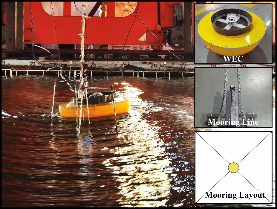
Table 1. Parameters of 1:16 model.
|
Mass |
128.25 |
kg |
|
Diameter |
1.00 |
m |
|
Height of COM |
0.30938 |
m |
|
MOI: Ixx |
1.2060 × 101 |
kg·m2 |
|
MOI: Iyy |
1.1632 × 101 |
kg·m2 |
|
MOI: Izz |
1.6610 × 101 |
kg·m2 |
COM: Center of mass, MOI: Moment of Inertia.
The wave tank is 60 m long and 36 m wide, located in the Shandong Provincial Key Laboratory of Ocean Engineering. The WEC was deployed 30 m away from the wave maker, as shown in Figure 3. A 4-leg mooring system was used in this experiment, with a misalignment angle of 45° relative to the incident waves.
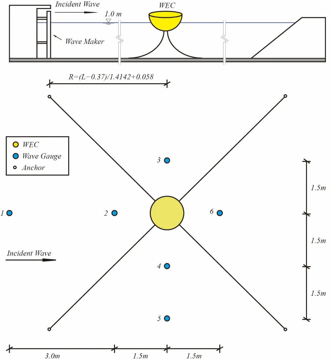
Figure 3. Sketch of experiment campaign.
The mooring system was originally designed in a water depth of 31.6 m, corresponding to 1.975 m in scaled ratio 1:16, while the maximum depth of the wave tank is 1 m, in which the equivalent mooring is required. The equivalent mooring system should not significantly change the restoring forces of the buoy within a specified offset range. Specifically, the horizontal tension should be consistent between the equivalent and original systems, because the restoring force in the horizontal direction is provided entirely by the mooring system. However, in the vertical direction, deviations in vertical tension are acceptable, as they are balanced by the hydrostatic restoring force. Therefore, the buoy’s draft variation is the main concern for judging the vertical tension differences.
The static catenary theory was adopted for the calculation in the design process, in which the line’s dynamic-related factors, like the drag forces, are neglected. Considering that the redundancy of the grounded segment is required, in other words, the angle between the line and the horizontal direction at its touchdown point (TDP) is zero, the standard form of the catenary equation is given by [28]:
|
```latex\begin{cases} x = \dfrac{H}{\omega}sinh^{-1}\left(\dfrac{L\omega}{H}\right)\\[6pt] z = \dfrac{H}{\omega}\left[cosh\left(\dfrac{\omega x}{H}\right)-1\right]\\[6pt] V = \omega L \end{cases}``` |
(1) |
Here, $$\omega$$ represents the submerged weight per unit length, and $$L$$ denotes the arc length from the TDP to a specified point at the suspended segment of the line (hereinafter, called catenary). H is the constant horizontal tension component along the line, and $$\mathrm{V}$$ is the vertical tension component at that point. The variables $$x$$ and $$z$$ denote the horizontal and vertical projection distances from the TDP to the specified point, respectively. These equations indicate the position and tension components at any point along the catenary, while in practical calculations, we focus on the top end of the line.
Given the weight, total length, and positions of the two endpoints of the line, the line tension can be obtained through an iterative procedure: (1) Assume an initial value of the suspended length and calculate the corresponding horizontal projection distance from the TDP to the top end. (2) Substitute these two values into the expression of $$x$$ and solve the implicit expression for the horizontal tension. (3) Substitute the result into the expression of $$z$$ to calculate the vertical projection distance from the TDP to the top end. (4) Update the suspended length and repeat the above steps until the calculated vertical projection distance converges to the actual vertical distance between the two endpoints.
In the equivalent mooring design, its line parameters were adopted from actual chains. By adjusting the line length and relative positions of the two endpoints, an equivalent mooring system with performance similar to that of the target mooring system was obtained, as shown in Table 2. It should be noted that the equivalent mooring line has a significantly higher in-water density, while the water depth, line length, and mooring radius are substantially reduced, making it possible to be deployed in the wave tank.
The theoretical horizontal tension of these two mooring systems in Figure 4a demonstrates good agreement. The vertical tension in Figure 4b demonstrates a deviation of approximately 50 N, whereas the drafts of the buoy under these two mooring systems are similar, as shown in Figure 4c.
The normalized error was adopted to evaluate the consistency of horizontal tension and the buoy’s draft, given by:
|
```latex{\epsilon }_{norm}=\frac{{Q}_{Eq}-{Q}_{Tar}}{{Q}_{ref}}×100\%``` |
(2) |
Here, the numerator on the right-hand side of the equation represents the absolute error between the equivalent and the target system. The denominator, $${Q}_{ref}$$, denotes the reference scale. For the comparison of horizontal tension, $${Q}_{ref}$$ is defined as the horizontal tension of the target system at the designed offset of 0.3 m. For the draft comparison, it is defined as the draft of the buoy without the mooring system. Figure 5 presents these two normalized errors, showing acceptable agreement between the equivalent mooring system and the original one. Therefore, this equivalent design was used in the experiment.
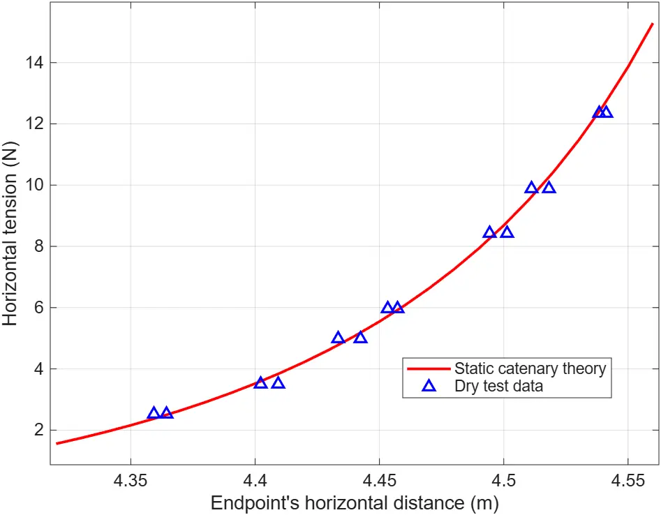
As the line of the equivalent mooring system corresponds to the actual chains, there is no need to adjust its weight except for the segments with sensors and connectors. The horizontal stiffness of the physical line model was measured by a dry test and compared with its theoretical curves, as shown in Figure 6.
Table 2. Line parameters in 1:16 scaled model.
|
Target Mooring |
Equivalent Mooring |
|
|---|---|---|
|
Water depth |
1.975 m |
1 m |
|
Line length |
20 m |
4.81 m |
|
In-water Density |
0.0608 kg/m |
1.7165 kg/m |
|
Mooring radius |
19.66 m |
4.44 m |
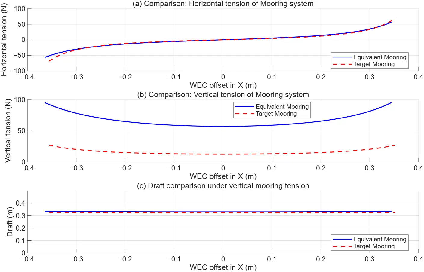
Figure 4. Comparison of the equivalent and target mooring system with respect to offset: (a) Horizontal tension of mooring system; (b) Vertical tension of mooring system; (c) Draft under vertical mooring tension.
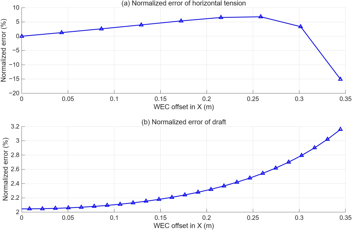
Figure 5. Normalized error assessment: (a) Normalized error of horizontal tension; (b) Normalized error of draft.
There are two full-scale numerical models corresponding to the equivalent mooring and the target mooring. The incident waves in these numerical models are generated by the scaled-up water surface elevation data measured from the wave calibration test. To be specific, the selected wave gauge was located in the position that was later used for the WEC.
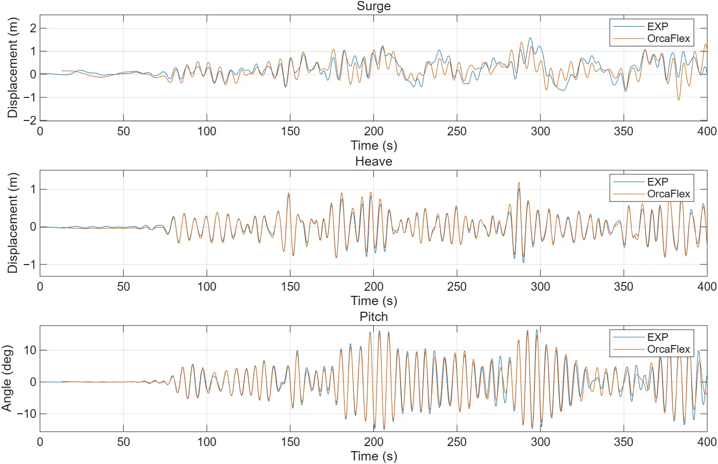
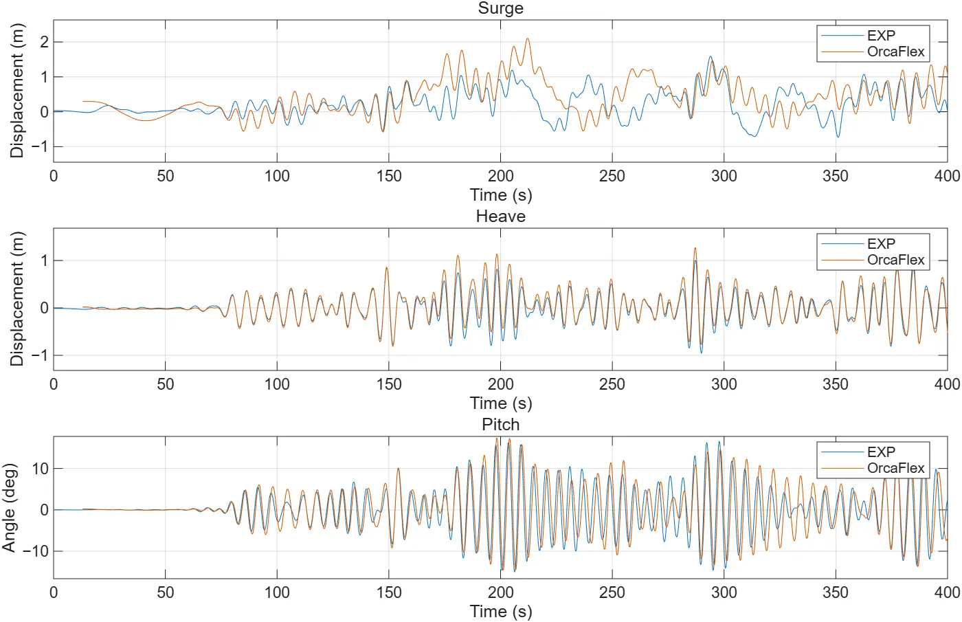
Figure 7a compares the numerical model in equivalent mooring with the scaled-up experiment data, with a peak period of 5.88 s and significant wave height of 1.52 m. It demonstrates good accuracy of the numerical simulation, where the heave and pitch motions are almost the same, while a small deviation occurred in the surge direction. This deviation is driven by the wave differences between the experiment and the numerical model. Specifically, in the experiment, the wave is inevitably reflected by the tank’s boundaries, which results in a multidirectional wave field. However, it is considered a unidirectional wave in the numerical model, although with the same series of surface elevations. Additionally, the surge motion, compared with heave and pitch, is more likely to be affected by wave directions.
On the other hand, the numerical model with target mooring was validated with the same incident wave, as shown in Figure 7b. The consistency is not as good as the previous one due to the following reasons: (1) Difference in water depth affects the buoy’s hydrodynamic results in the frequency domain. (2) The dynamic characteristics of the line are different, for example, the inertia and drag force of line segments. Although with some deviations, this model also agrees well with the experiment.
According to these two comparisons, the numerical model possesses a good ability to accurately predict the WEC’s response. It will play a major role in the following mooring design and optimization process.
 |
|
(a) |
 |
|
(b) |
Figure 7. Numerical model validations. (a) Comparison of numerical model (Equivalent mooring) and experiment data in full-scale; (b) Comparison of numerical model (Target mooring) and experiment data in full-scale.
2.3. Mooring Optimization
2.3.1. Environment Information
It is well known that the extreme line tension driven by the extreme sea states significantly threatens the survivability of a floating structure. For a floating WEC, the waves, tides, and currents are the dominant environmental conditions and should be carefully considered.
The area to the south of Pingtan Island with a water depth of 31.6 m was selected. The corresponding environmental information was acquired from reanalysis data; specifically, the wave and current data were obtained from the Copernicus Marine service [29,30], while the tide data were provided by the Climate Data Store [31]. The data time span is 32 years, starting from 1 January 1993 and ending with 31 December 2024. It is noted that the data of wave, current, and tide were obtained from different places, while these locations are spatially close to each other.
The Direct-IFORM [32] is adopted to calculate the 2D environmental contours of extreme wave height and period. The wave data were categorized into 4 groups by direction, and their environmental contours were calculated separately, as shown in Figure 8. It is noted that a declustering process should be conducted in advance, with a window of 48 h. The mean wave directions with their fractions are listed in Table 3.
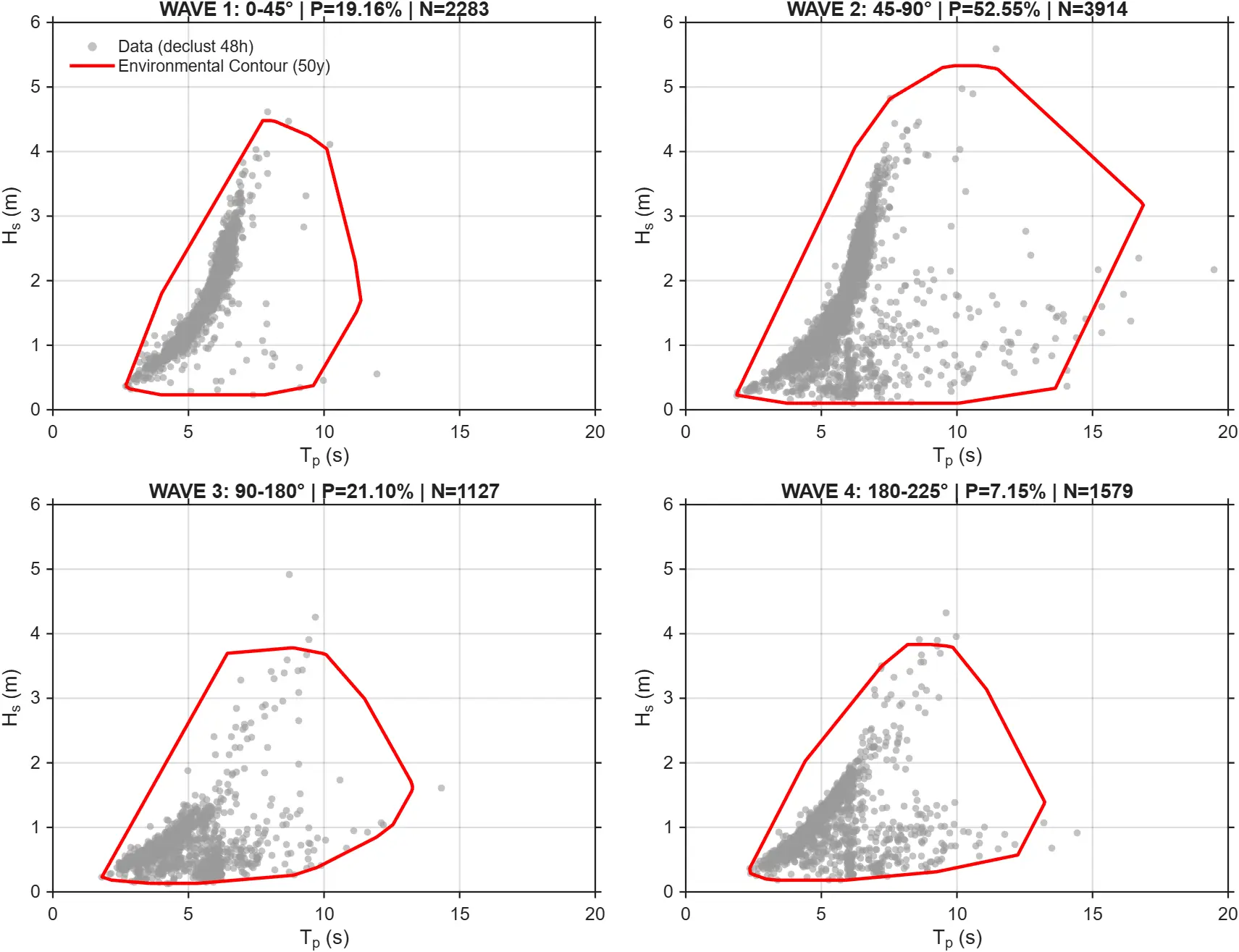
Table 3. Direction of extreme waves.
|
Components |
Azimuth Range |
Mean Azimuth |
Percentage |
|---|---|---|---|
|
WAVE 1 |
[0, 45) |
37.88° |
19.16% |
|
WAVE 2 |
[45, 90) |
56.65° |
52.55% |
|
WAVE 3 |
[90, 180) |
158.86° |
7.15% |
|
WAVE 4 |
[180, 225) |
191.60° |
21.10% |
The extreme tide level is defined as the sum of the astronomical tide and storm surge according to DNVGL-OS-E301 [33]. The astronomical tide is driven by the gravity of the Earth, Moon, and Sun and varies periodically. In this study, the highest and lowest astronomical tide levels were determined from the 90th percentile (P90) and the 10th percentile (P10) of its time series, respectively. In contrast, the storm surge driven by the weather is considered a random distribution. Thus, the GEV distribution is adapted to obtain its extreme value at the return period of 50 years. In summary, the extreme high and low tide levels are 35.049 m and 28.866 m, respectively.
In terms of extreme current, it is noted that the maximum current may not simultaneously occur with extreme wave or tide levels. Therefore, the storm event analysis is adopted, and the process of extreme current design is: (1) Obtain thresholds: Analyzing the series of storm surges and obtaining its P10 and P90 as the threshold storm set-up and storm set-down. (2) Identify the storm event through these thresholds, and the adjacent events with a time gap of less than 48 h should be integrated since the storms usually last more than 2 days. (3) Observation window: extend the window for 12 h before and after the storm event, and then record the maximum current speed as well as its direction. (4) Obtain extreme current: fit the current speed samples with the GEV distribution, and finally calculate the extreme current speed for a specific return period.
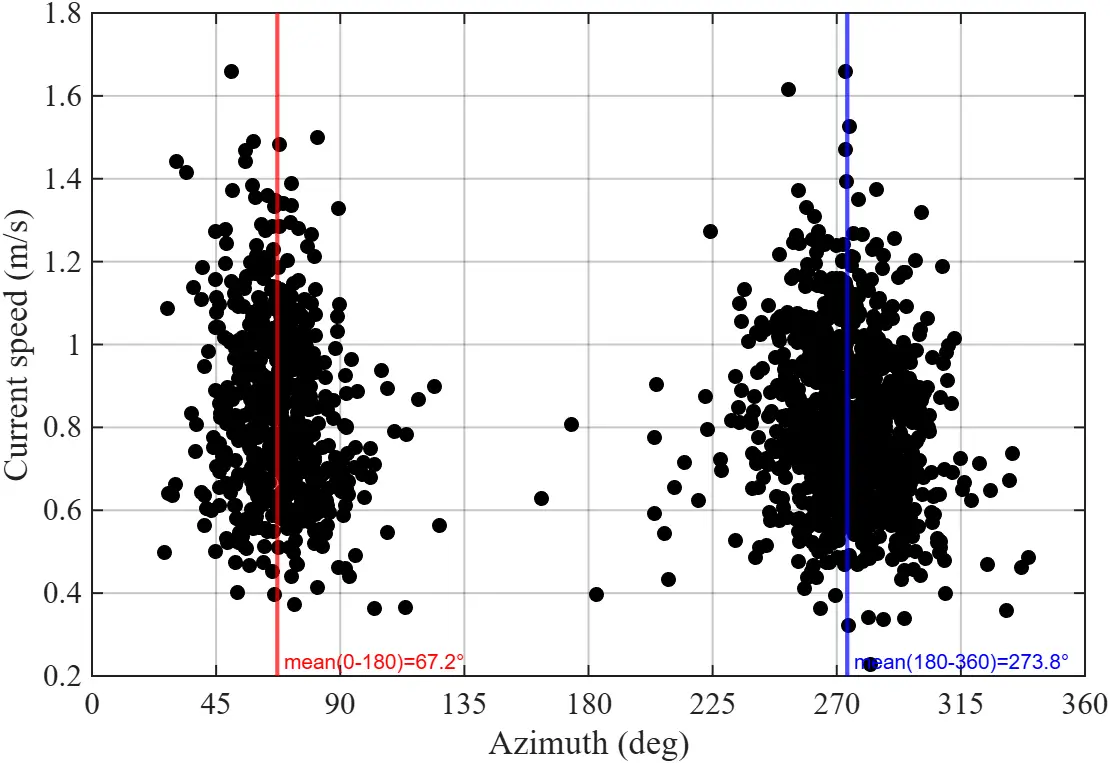
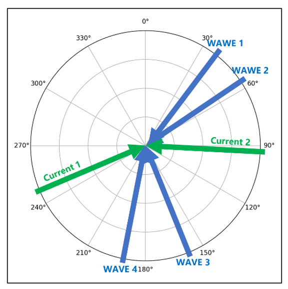
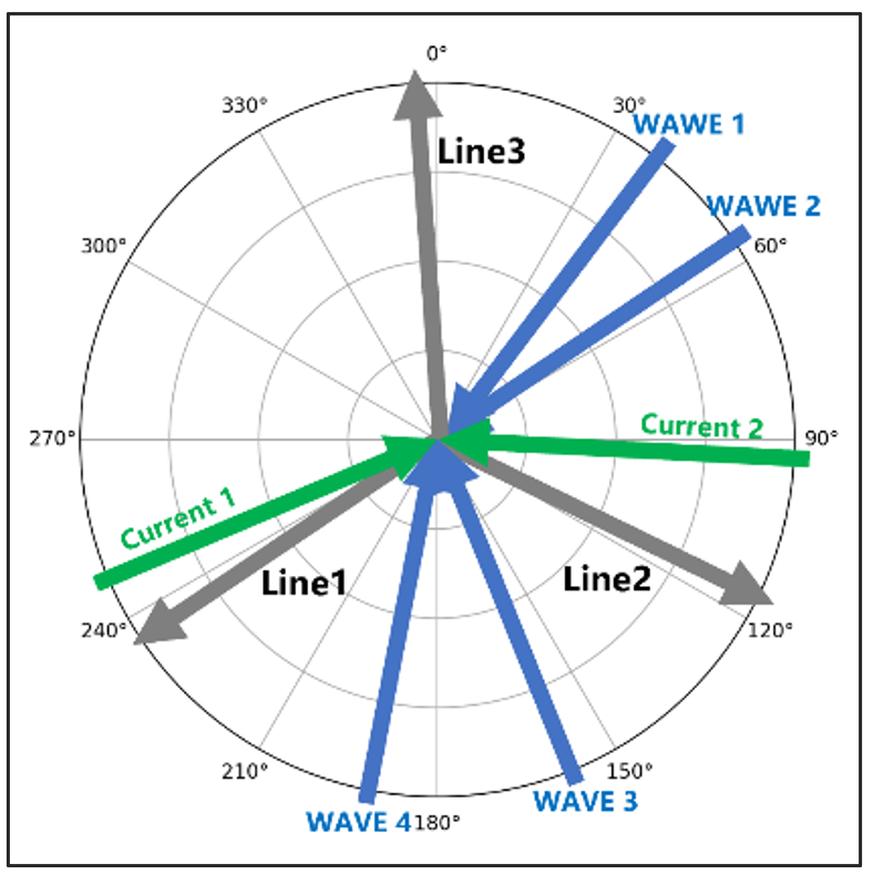
The distribution of the identified maximum currents in Figure 9 demonstrates two distinct directions; therefore, two currents were considered in extreme sea states: Current1 at azimuth 67.2° with speed 1.647 m/s and Current2 at azimuth 273.8° with speed 1.647 m/s. Figure 10 demonstrates the azimuth of extreme waves and currents.
As for the operational sea state, some assumptions are made for simplification and conservative design: (1) The misalignment of wave and current is neglected. (2) The water depth in operational sea states is considered only at the mean surface level (MSL). The operational sea states are summarized in Table 4.
Table 4. Operational sea state.
|
Ocase |
Water Depth |
Hs (m) |
Tp (s) |
Current (m/s) |
Percentage (%) |
|---|---|---|---|---|---|
|
1 |
31.6 |
1.810 |
6.130 |
0.211 |
9.747 |
|
2 |
1.420 |
5.430 |
0.151 |
9.643 |
|
|
3 |
0.960 |
5.250 |
0.193 |
9.625 |
|
|
4 |
0.830 |
4.360 |
0.284 |
9.539 |
|
|
5 |
1.700 |
5.800 |
0.223 |
9.036 |
|
|
6 |
2.650 |
6.550 |
0.445 |
8.966 |
|
|
7 |
2.090 |
6.180 |
0.322 |
7.770 |
|
|
8 |
2.290 |
6.280 |
0.355 |
6.382 |
|
|
9 |
0.610 |
3.540 |
0.313 |
5.966 |
|
|
10 |
1.280 |
5.040 |
0.168 |
5.307 |
2.3.2. Layout and Orientation
The mooring system in the experiment is used for concept research and validating numerical models, it is obviously not the ideal design. The 4-leg layout lacks safety redundancy in case of an accidental state. If one line fails, the remaining 3 lines will fail one by one due to the asymmetric tension between them. In contrast, a 3-leg design performs better in single-line failure because the even number of the remaining line has smaller tension differences when the system reaches a new balance. Therefore, a 3-leg layout was adopted for the mooring system.
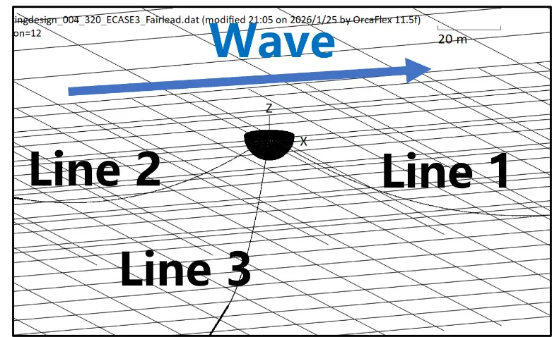
As for the mooring orientation, it is considered to align with the strongest extreme wave, WAVE 2, which accounts for over 50% of the total waves and has the most violent environmental contours, as shown in Figure 8. The determined layout and orientation are shown in Figure 11.
 |
 |
|
(a) |
(b) |
Figure 11. Sketch of mooring orientation: (a) Azimuth of mooring lines; (b) Mooring Line number.
2.3.3. Fairlead Position
The line tension is highly dependent on the displacement of the fairlead end connecting to the WEC [34]. Therefore, it is reasonable to adjust the fairlead position on the WEC to improve mooring performance. As shown in Figure 12, the fairlead was originally placed close to the WEC’s bottom in the experiment. When the WEC rides in the wave, the majority of fairlead end displacements are contributed by the equivalent translational displacements of pitch motion. And these equivalent translational displacements are mainly in the horizontal direction. On the contrary, if the fairlead position is located at a higher position, its equivalent translational displacements are mainly in the vertical direction. These two situations are quite different because catenaries are usually more sensitive to the horizontal motion of their top end, therefore, a higher fairlead position may lead to relatively smaller excitations to mooring lines and lower tension.
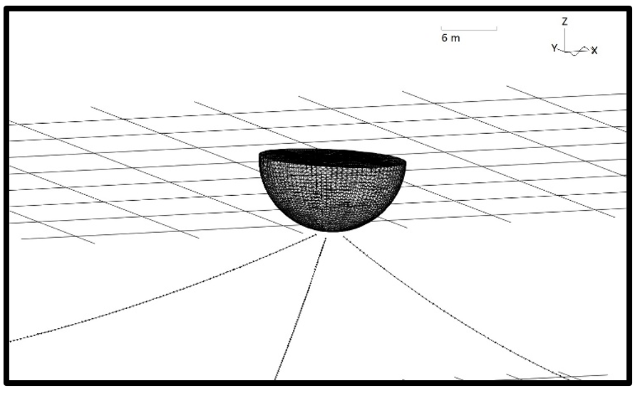
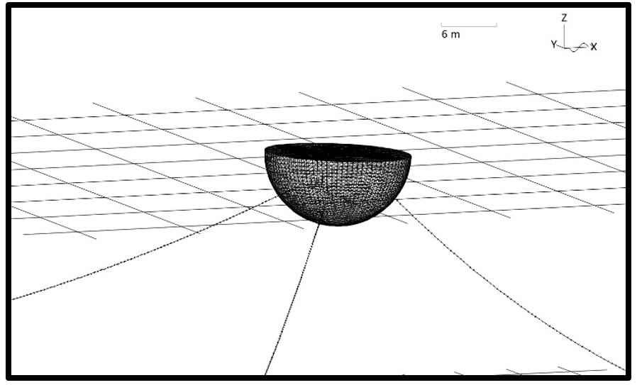
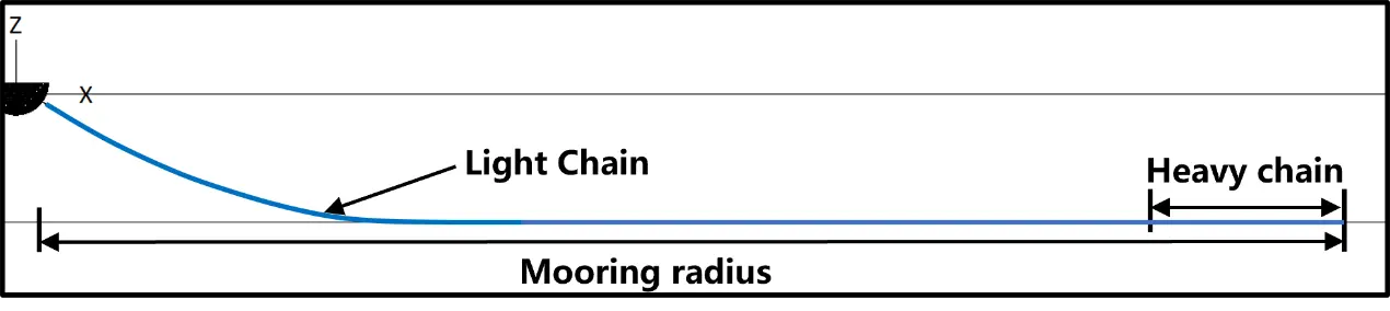
Figure 13 demonstrates the initial design of mooring lines in catenaries, which consists of a studless light chain and an additional studlink heavy chain to its bottom end. The heavy chain provides more redundant stiffness by its weight in order to avoid the anchor being lifted up and help reduce mooring radius (horizontal distance from fairlead end to anchor point) in the later adjustment. Compared with the studlink chain, the studless chain is more flexible and cost-effective at the same strength, therefore, it is adopted as the main component.
Line parameters of this line corresponding to the original and new fairlead positions are listed in Table 5, namely Mooring1a and Mooring1b, respectively. It is noted that their pretensions were evaluated in MSL, ignoring wave and current loads, controlled by adjusting the light chain length.
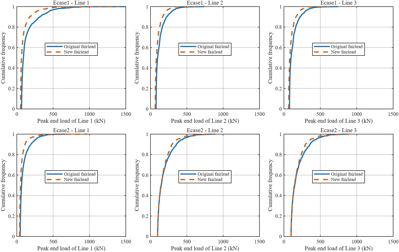
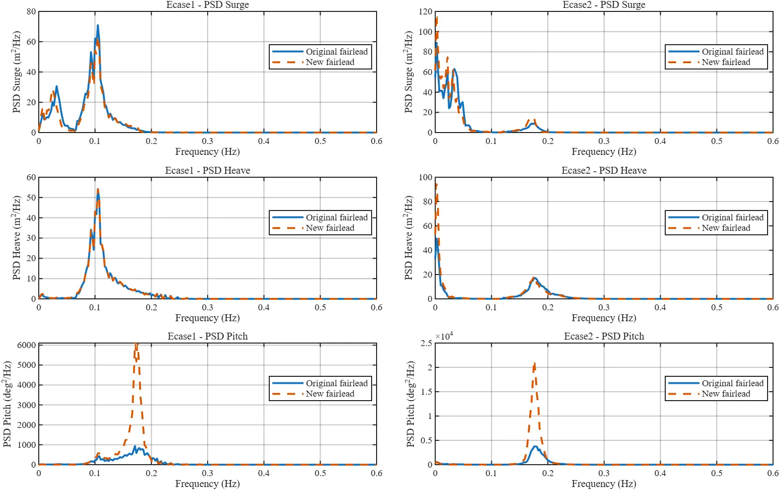
The tension comparisons are shown in Figure 14 in the form of cumulative density (CDF) of peak load. It is obvious that the new fairlead significantly reduces the line’s overall tension. Besides, it also enhances the pitch motion, as shown in Figure 15. Furthermore, the extreme values listed in Table 6 illustrate that the extreme loads and offsets are reduced by this new fairlead as well.
2.3.4. Line Parameters
To further reduce the extreme load, two elastic ropes were added, as shown in Figure 16. The polyester is connected to the WEC’s fairlead to utilize its good abrasion resistance and corrosion resistance to reduce fatigue damage near the fairlead end. As for nylon, its good elasticity is utilized to reduce snap load.
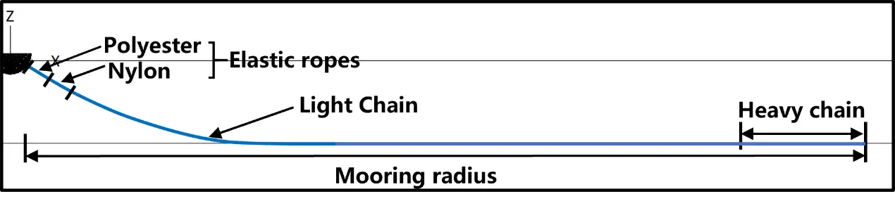
The design of this hybrid line initially considered the axial stiffness of polyester and nylon as linear, labelled as Mooring2a in Table 5 and Table 6. Compared with the catenary line Mooring1b, a significant reduction in extreme load and extreme offset is observed.
Considering the high elastic feature of nylon may lead to significant deviation between linear and nonlinear axial stiffness, it is more realistic to consider it in nonlinear form. Figure 17 compares the axial tension-strain curve of linear (Nylon1) and nonlinear (Nylon2) axial stiffness. Also, an optimized curve (Nylon3) is proposed to further reduce snap load. These three mooring systems are named respectively as Mooring2a, Mooring2b, and Mooring3c in Table 5. Their numerical results in Table 6 indicate that the ideal linear axial stiffness indeed underestimates the extreme load, while the optimized stiffness Nylon3 performs better than Nylon2, indicating that the modification of nonlinear axial stiffness makes sense.
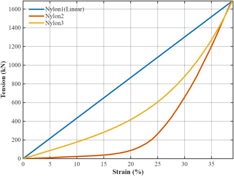
The minimum breaking load (MBL) of the light chain used in Mooring2c is 1279.49 kN for the commonly used Grade3 chain. In the preliminary design, its design capacity is roughly evaluated as 727.85 kN by the expression below:
|
```latex\mathrm{Capacity} = \mathrm{MBL} * 0.95 / 1.67``` |
(3) |
According to the simulation results, the extreme tension of Mooring3c is close to the light chain’s capacity even at mean sea level (MSL) without any current loads. A stronger chain is required, as the line should be considered at the highest sea level (HSL) and under extreme current conditions.
In the following design, namely Mooring2d, the light chain bar diameter is increased, and the simulations take HSL and extreme currents into consideration. The line parameters and simulation results are summarized in Table 5 and Table 6. The results indicate that the on-bottom length is insufficient for harsher environments, and that tensions in some cases are extremely high.
To tackle this problem, both line geometry and line strength should be adjusted. Considering the fact that higher tensions are partly contributed by the insufficient line length, the geometry optimization was carried out first. An extra 40 m long heavier studlink chain with a larger bar diameter is added, and the mooring radius is extended, it is labelled as Mooring3a in Table 5. Simultaneously, the same configuration with higher pretension, namely Mooring3b and Mooring3c, are analyzed and compared as well. It is noted that the pretension rise of these two moorings is achieved by simultaneously reducing the light chain length of all three lines. The two risky sea states, “Ecase1+Current1” and “Ecase2+Current2”, were applied for evaluating these three mooring systems, as shown in Table 6. The results illustrate that increasing pretension can make the front side Line2 safer in “Ecase2+Current2” but, on the contrary, deteriorates the load of the back side Line1 in “Ecase1+Current1”.
The wave Ecase2 corresponds to the pitch natural period, in which the response is dominated by pitch motion. The violent pitch response, together with the low-frequency drift, leads to a large-amplitude tension variation, therefore, other DOFs such as yaw are amplified by it, especially in misalignment excitations (Current2). When these effects are positively superimposed at a moment, an extremely high tension occurs. Hence, the increasing pretension can weaken yaw motion and reduce the maximum load.
On the contrary, WEC responses in Ecase1 are more about low-frequency drift in the surge direction as the wave frequency deviates from the pitch natural frequency but gets closer to the frequency of the mooring system. In other words, the maximum offsets play an important role in this sea state. What’s more, increasing line pretension further broadens the tension gap between the same offset in positive and negative directions, making the stern side Line1 more likely to experience higher tension. When this system confronts the excitation from the back side (Current1), this shortcoming is fully exposed and then leads to extremely high tension in Line1.
According to these characteristics, the following mooring system (Mooring3d) adjusts the line pretension in a different way that only decreases line length on the bow side while the stern line remains the same, as shown in Table 5, where the light chain in the later designs has two different lengths. The results in Table 6 indicate that such an adjustment makes little contribution to improving extreme loads, while the extreme offsets are reduced.
According to Table 5 and Table 7, the capacity of polyester, nylon, and light chain in Mooring3d are 969.72 kN, 959.23 kN, and 1114.97 kN, respectively, which is no longer appropriate for their extreme loads in Table 6. Therefore, these segments were enhanced in Mooring4. However, the increasing MBL will inevitably weaken the lines’ elasticity, especially for nylon, and then weaken the line’s ability to reduce snap load. The axial stiffness of the stronger nylon (Nylon31) is compared with the previous one (Nylon3) in Figure 18. For the nylon with higher MBL, the slope of the axial stiffness curve is steeper, especially in high tension.
The line parameters and simulation results for Mooring4 are listed in Table 5 and Table 6. The maximum extreme load 1682.4 kN slightly exceeds its capacities listed in Table 7, while the elastic ropes were not strengthened further because the environmental conditions mentioned above are conservatively designed, as the correlation of wave and current is not considered due to insufficient data. However, for the light chain that would suffer from corrosion and MBL decrease, a larger bar diameter is needed.
Through a series of optimizations, the preliminary design of the mooring system, namely Mooring5, is finally obtained, and it is evaluated in the next step, the code check. It should be noted that further optimizations may be required according to the code check results.
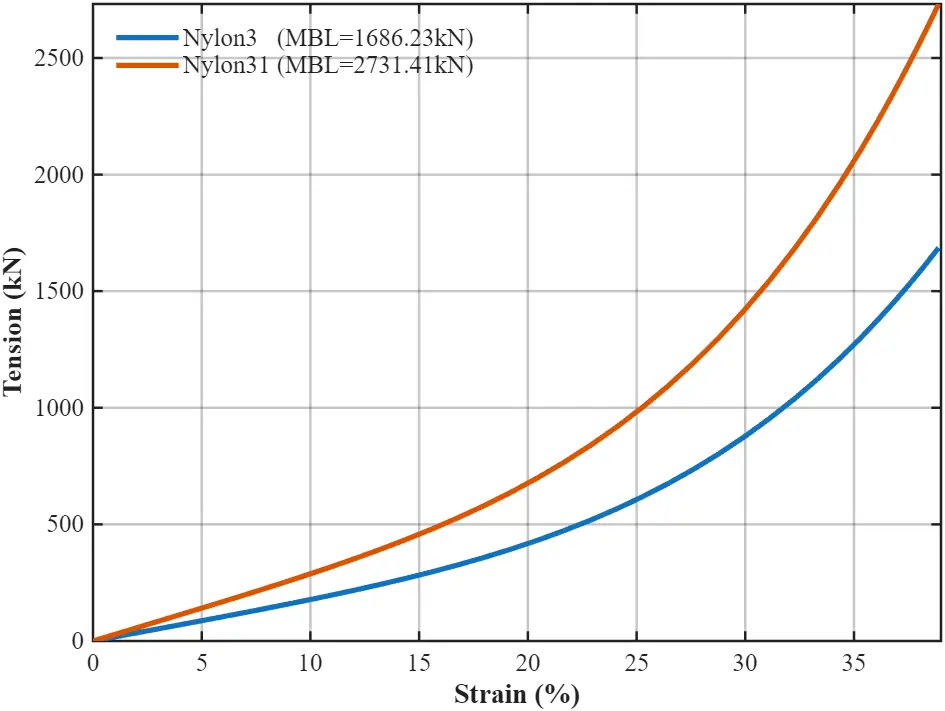
Table 5. Summary of mooring parameters in preliminary design process.
|
Name |
```latex{\bm{T}}_{\bm{p}\bm{r}\bm{e}\bm{t}}``` (kN) |
Elastic Ropes Diameter (mm), Axial Stiffness (kN) |
Chains Diameter (mm), Length (m) |
Mooring Radius (m) |
||||||||
|---|---|---|---|---|---|---|---|---|---|---|---|---|
|
Polyester (10 m) |
Nylon (10 m) |
Light Chain |
Heavy Chain1 |
Heavy Chain2 |
||||||||
|
Mooring1a |
50 |
\ |
40 |
274.6 |
80 |
50 |
\ |
320 |
||||
|
Mooring1b |
275.6 |
|||||||||||
|
Mooring2a |
50 |
100 |
10.9 × 10³ |
110 |
Nylon1 |
40 |
175.0 |
80 |
50 |
\ |
240 |
|
|
Mooring2b |
Nylon2 |
173.6 |
||||||||||
|
Mooring2c |
Nylon3 |
175.0 |
||||||||||
|
Mooring2d |
Nylon3 |
50 |
176.4 |
|||||||||
|
Mooring3a |
50 |
100 |
10.9 × 10³ |
110 |
Nylon3 |
50 |
176.4 |
80 |
50 |
100 |
40 |
280 |
|
Mooring3b |
75 |
175.1 |
||||||||||
|
Mooring3c |
100 |
174.1 |
||||||||||
|
Mooring3d |
80 |
176.4 174.1 |
||||||||||
|
Mooring4 |
80 |
130 |
18.42 × 10³ |
140 |
Nylon31 |
60 |
176.4 175.9 |
80 |
50 |
100 |
40 |
280 |
|
Mooring5 |
80 |
130 |
18.42 × 10³ |
140 |
Nylon31 |
70 |
177.5 177.0 |
80 |
50 |
100 |
40 |
280 |
Tips: $${T}_{pret}$$: Pretension in the line’s top end (Evaluated at Mean Sea Level without wave & current), it is controlled by adjusting light chain length; Mooring radius: horizontal distance from fairlead to anchor; Mooring3d~Mooring5 have longer front lines than that in the back, therefore, two light chain lengths are listed; Nylon1 represents the ideal linear axial stiffness, and Nylon2~Nylon31 correspond to the nonlinear stiffness.
Table 6. Summary of inputs and results in the process of preliminary design.
|
Name |
Wave & Current |
Tide |
Min On-Bottom Length (kN) |
Max Load at Top End (kN) |
Offset (m) |
|||||
|---|---|---|---|---|---|---|---|---|---|---|
|
Line 1 |
Line 2 |
Line 3 |
Line 1 |
Line 2 |
Line 3 |
−X |
+X |
|||
|
Mooring1a |
Ecase1 |
MSL |
39 |
33.5 |
33.5 |
1731.1 |
742.62 |
742.77 |
−4.7573 |
9.7060 |
|
Ecase2 |
111.52 |
22 |
22 |
671.31 |
889.66 |
889.68 |
−2.1399 |
9.6749 |
||
|
Mooring1b |
Ecase1 |
42 |
47 |
47 |
1413.6 |
628.95 |
628.84 |
−4.7664 |
8.7469 |
|
|
Ecase2 |
84.475 |
22 |
22 |
968.16 |
894.10 |
894.12 |
−1.9675 |
8.8889 |
||
|
Mooring2a |
Ecase1 |
MSL |
46 |
44.5 |
44.5 |
461.52 |
328.38 |
328.36 |
−4.4407 |
6.9841 |
|
Mooring2b |
Ecase1 |
MSL |
23.5 |
36.5 |
36.5 |
973.02 |
459.48 |
459.44 |
−4.5985 |
7.8364 |
|
Mooring2c |
Ecase1 |
MSL |
39 |
41 |
41 |
681.59 |
385.11 |
351.1 |
−4.2303 |
7.0151 |
|
Mooring2d |
Ecase1+Current1 |
HSL |
NaN |
74.985 |
57.995 |
1139.3 |
320.21 |
378.24 |
−6.8195 |
4.2781 |
|
Ecase2+Current1 |
28.999 |
80.482 |
62.992 |
1045.6 |
341.67 |
374.56 |
−3.3686 |
3.3929 |
||
|
Ecase1+Current2 |
101.98 |
NaN |
43.999 |
274.36 |
837.39 |
427.29 |
−1.9609 |
10.596 |
||
|
Ecase2+Current2 |
91.975 |
NaN |
NaN |
249.93 |
1837.1 |
1000.5 |
−2.3948 |
15.149 |
||
|
Mooring3a |
Ecase1+Current1 |
HSL |
54.999 |
114.49 |
97.995 |
1132.5 |
319.05 |
376.72 |
−6.823 |
4.2602 |
|
Ecase2+Current2 |
132.48 |
4.499 |
25.499 |
239.37 |
1821.8 |
987.91 |
−2.3629 |
14.636 |
||
|
Mooring3b |
Ecase1+Current1 |
36.799 |
86.499 |
80.999 |
1393.3 |
462.34 |
518.21 |
−6.8805 |
4.9894 |
|
|
Ecase2+Current2 |
98.303 |
5.999 |
27.999 |
302.16 |
1468.7 |
953.91 |
−2.3015 |
12.798 |
||
|
Mooring3c |
Ecase1+Current1 |
22.799 |
69.499 |
63.499 |
1698.6 |
622.51 |
680.84 |
−7.165 |
5.8346 |
|
|
Ecase2+Current2 |
89.299 |
14.499 |
13.499 |
650.71 |
1155.7 |
1058.6 |
−1.5231 |
12.327 |
||
|
Mooring3d |
Ecase1+Current1 |
34.999 |
83.499 |
77.499 |
1418.3 |
492.76 |
547.56 |
−8.338 |
3.6144 |
|
|
Ecase2+Current2 |
102.49 |
5.999 |
24.999 |
382.09 |
1457.1 |
967.83 |
−3.5225 |
11.566 |
||
|
Mooring4 |
Ecase1+Current1 |
HSL |
38 |
90 |
87.5 |
1682.4 |
550.29 |
610.57 |
−7.2032 |
4.8823 |
|
Ecase2+Current2 |
138.47 |
10.5 |
39.5 |
354.48 |
1337.5 |
1009.3 |
−2.182 |
12.113 |
||
Tips: The duration of these full-scaled simulation is 3 h; Min on-bottom length represents the minimum line length between touchdown point and anchor throughout the simulation, and “NaN” indicates that the anchor is lifted up during the simulation. The offset corresponds to incident WAVE 2, where +X represents wave direction and −X indicates the reverse direction. The waves were selected from the environmental contours of WAVE 2, and Ecase1 represents the wave with maximum wave height (Hs = 5.33 m, Tp = 9.91 s), while Ecase2 corresponds to the pitch natural period that varies in different mooring designs.
Table 7. Properties of line components.
|
Components |
Diameter (mm) |
MBL (kN) |
Capacity (kN) |
|---|---|---|---|
|
Polyester |
100 |
1704.67 |
969.72 |
|
130 |
2880.89 |
1638.83 |
|
|
Nylon |
110 |
1686.23 |
959.23 |
|
140 |
2731.41 |
1553.80 |
|
|
Chain |
40 |
1279.49 |
727.85 |
|
50 |
1960.0 |
1114.97 |
|
|
60 |
2765.95 |
1573.44 |
|
|
70 |
3687.94 |
2097.93 |
|
|
80 |
4716.54 |
2683.06 |
|
|
100 |
7056.0 |
4013.89 |
2.3.5. Code Check
In the design of Mooring5, the heave natural period is 4.99 s and the pitch natural period is 5.61 s (HSL) and 5.71 s (MSL, LSL), then the extreme waves corresponding to this mooring system were designed based on the environmental contours in Figure 8, and the detailed information is listed in Table 8. The extreme sea states consist of 3 tide levels, 2 currents, 4 wave directions, and 12 waves per direction, which sum to 288 cases. Therefore, it is necessary to compare and identify the critical cases in advance to reduce computational cost.
The simulations for comparison are considered in 600 s, and they are no longer compared by maximum loads but by a new indicator:
|
```latex{I}_{0.9}={\int }_{0.9}^{1.0}TdF\left(T\right)``` |
(4) |
Here $$F\left(T\right)$$ is the Cumulative Distribution Function (CDF) of the mooring line’s peak load in the riskiest mooring line, corresponding to the rightmost curve in Figure 19b. The peak loads are identified from the tension series, as shown in Figure 19a. The indicator $${I}_{0.9}$$ represents the area surrounded by $$F\left(T\right)$$, T = 0, $$F=0.9$$ and $$F=1.0$$ in the coordination of $$T-F\left(T\right)$$, its definition is also illustrated in Figure 19c.
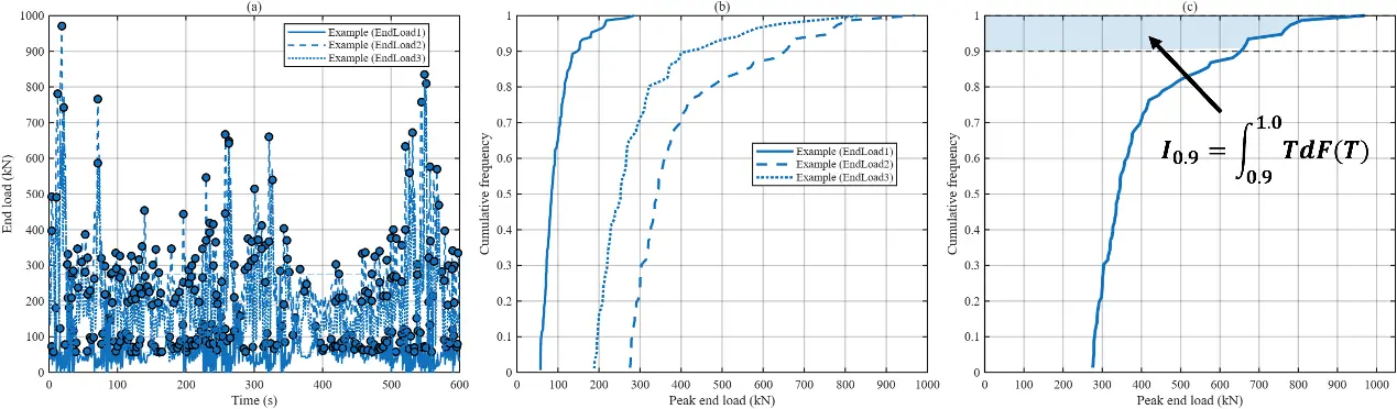
Figure 19. Sketch of the new indicator: (a) Peak load identification; (b) Peak load CDF; (c) Area of $${I}_{0.9}$$.
Firstly, the comparison is conducted among different tide levels, and three representative extreme sea states corresponding to the maximum wave height (Ecase1), pitch frequency (Ecase2), and heave frequency (Ecase3) were selected, as shown in Figure 20. The comparison illustrates that the cases in HSL normally have higher tension. Secondly, all extreme sea states in HSL are compared, as shown in Figure 21, which illustrates that risky sea states mostly appear in WAVE 2. Thirdly, the comparison within WAVE 2 and HSL, as shown in Figure 22, with extra waves whose period is close to the pitch natural period, namely Ecase25~Ecase29, with an interval of 0.02 rad/s. Through this comparison, Ecase27 ($${H}_{s}$$ = 3.99 m, $${T}_{P}$$ = 6.16 s) with Current2 (azimuth = 273.8° speed = 1.647 m/s) is identified as the critical sea state, it corresponds neither to the sea state with the maximum significant wave height nor to the sea state associated with the natural period of pitch or heave.
In the ULS code check, the critical sea state was simulated using 10 different random seeds, each lasting 3 h. The maximum tensions obtained from each simulation and the mean value $$\mu$$ and standard deviation $$\sigma$$ corresponding to these 10 cases are listed in Table 9. The Most Probable Maximum (MPM) line tension $${T}_{MPM}$$ and the characteristic environmental tension $${T}_{C-env}$$ were adopted to evaluate the characteristic line tension, following the ULS criteria in DNVGL-OS-E301(Edition July 2018) [33], chapter 2 section 2 (2.2.8) and (2.5.2), respectively:
|
```latex{T}_{MPM}=\mu -0.45\sigma``` |
(5) |
|
```latex{T}_{C-env}={T}_{MPM}-{T}_{pret}``` |
(6) |
The design equation for ULS, obtained from chapter 2 section 2 (4.2.1) [33], is given by:
|
```latex{S}_{c}-{T}_{pret}{\gamma }_{pret}-{T}_{C-env}{\gamma }_{env}>0``` |
(7) |
Here, $${\gamma }_{pret}$$ and $${\gamma }_{env}$$ are the partial safety factors, for permanent structures, they are recommended as 1.20 and 1.45, respectively. This design equation can also be used for ALS, in which the safety factors decrease to 1.0 and 1.1, respectively. These safety factors corresponding to ULS and ALS are respectively obtained from chapter 2 section 2 (4.2.1) and (4.3.1) of the standard [33]. $${T}_{pret}$$ is the line pretension without the effect of wave, current, and wind. $${S}_{c}$$ is the design capacity (characteristic strength), a 100% corrosion allowance should be included for the chain segments:
|
```latex{S}_{c}\approx {S}_{mbs}\cdot {\left(\frac{{D}_{corr}}{{D}_{new}}\right)}^{2}``` |
(8) |
This equation corresponds to the chapter 2 section 2 (5.2.2) [33], where $${S}_{mbs}$$ represents the minimum breaking load (MBL) in engineering. $${D}_{new}$$ is the bar diameter of the chain and $${D}_{corr}$$ is the corroded bar diameter, given by:
|
```latex{D}_{corr}={D}_{new}-{r}_{corr}{T}_{D}``` |
(9) |
Here, $${T}_{D}$$ is the design service life of the mooring system. $${r}_{corr}$$ is the corrosion rate, and $$0.4\,\mathrm{ }\mathrm{m}\mathrm{m}/\mathrm{y}\mathrm{e}\mathrm{a}\mathrm{r}$$ is selected, following the recommended value listed in chapter 2 section 2 (5.2.1) of the DNVGL-OS-E301 (Edition July 2018) [33].
The ULS code check for the riskiest line, Line 2, is listed in Table 10, indicating that this mooring system can withstand extreme loads after 30 years of corrosion.
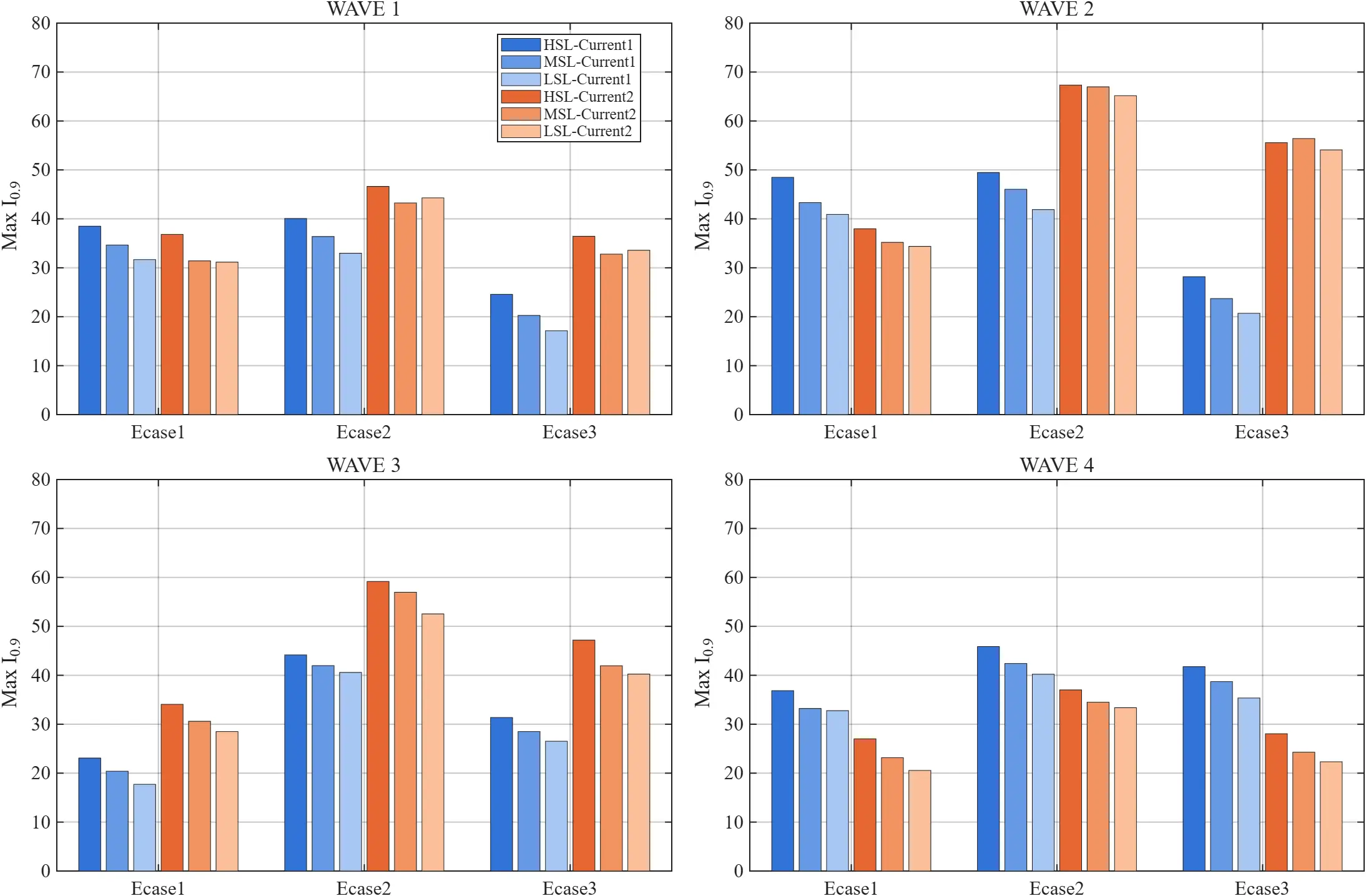
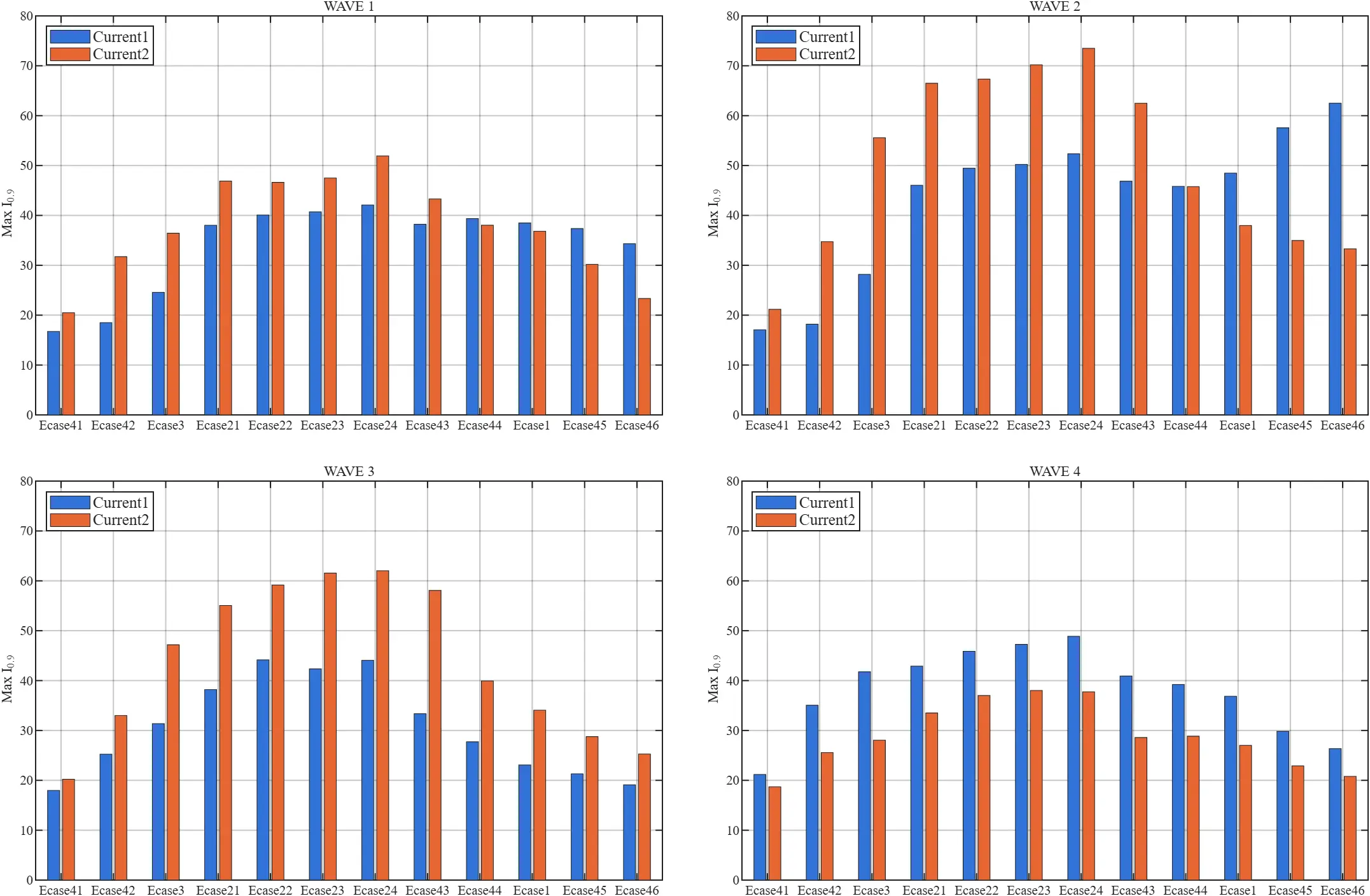
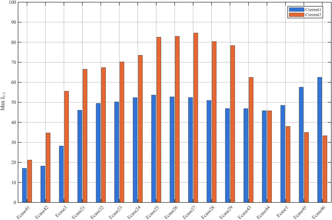
Table 8. Extreme waves (50y return period).
|
CASE NAME |
Categories |
[0, 45) |
[45, 90) |
[90, 180) |
[180, 225) |
||||
|---|---|---|---|---|---|---|---|---|---|
|
Hs |
Tp |
Hs |
Tp |
Hs |
Tp |
Hs |
Tp |
||
|
Ecase1 |
Max Hs |
4.48 |
7.74 |
5.33 |
9.91 |
3.78 |
8.80 |
3.83 |
8.18 |
|
Ecase21 |
Pitch |
2.88 |
5.51 |
3.42 |
5.51 |
3.00 |
5.51 |
2.60 |
5.51 |
|
Ecase22 |
2.95 |
5.61 |
3.51 |
5.61 |
3.08 |
5.61 |
2.66 |
5.61 |
|
|
Ecase23 |
3.02 |
5.71 |
3.60 |
5.71 |
3.15 |
5.71 |
2.71 |
5.71 |
|
|
Ecase24 |
3.10 |
5.82 |
3.70 |
5.82 |
3.24 |
5.82 |
2.77 |
5.82 |
|
|
Ecase3 |
Heave |
2.51 |
4.99 |
2.97 |
4.99 |
2.61 |
4.99 |
2.33 |
4.99 |
|
Ecase41 |
Others |
1.20 |
3.45 |
1.16 |
2.92 |
1.02 |
2.86 |
1.08 |
3.24 |
|
Ecase42 |
1.95 |
4.22 |
2.06 |
3.95 |
1.82 |
3.93 |
1.79 |
4.11 |
|
|
Ecase43 |
3.56 |
6.46 |
4.61 |
7.18 |
3.69 |
6.43 |
3.19 |
6.63 |
|
|
Ecase44 |
4.02 |
7.1 |
5.07 |
8.55 |
3.74 |
7.62 |
3.56 |
7.40 |
|
|
Ecase45 |
4.33 |
8.94 |
5.27 |
11.51 |
3.68 |
10.07 |
3.79 |
9.84 |
|
|
Ecase46 |
3.96 |
10.15 |
4.24 |
14.17 |
2.99 |
11.50 |
3.14 |
11.09 |
|
Table 9. Tension results of 3 h simulation.
|
$$\bm{\mu }$$ (kN) |
$$\boldsymbol{\sigma}$$ |
|
|---|---|---|
|
End load 1 |
252.37 |
28.36 |
|
End load 2 |
1698.33 |
174.61 |
|
End load 3 |
1272.46 |
188.12 |
Table 10. ULS code check.
|
MBL |
$$\boldsymbol{T_D}$$ |
Result |
|
|---|---|---|---|
|
Light chain (Grade 3) |
3687.94 |
30 |
210.99 > 0 |
|
Polyester |
2880.89 |
559.99 > 0 |
|
|
Nylon |
2731.41 |
410.51 > 0 |
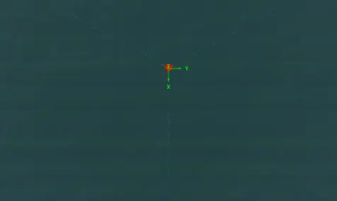
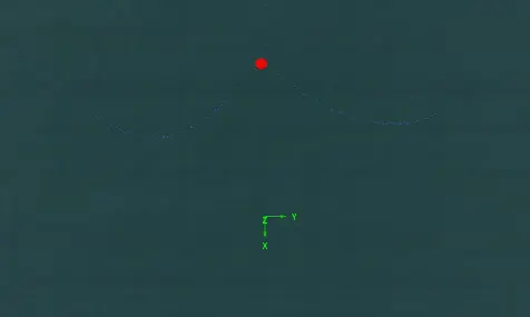
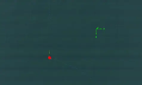
As for the ALS check, the critical case identification is simplified: (1) The comparing range is reduced to WAVE 2 in HSL. (2) The failed line is assumed to be the one with the highest tension in ULS, to be specific, assuming Line1 fails in Current1, and Line2 fails in Current2, as shown in Figure 23. The comparison in Figure 24 demonstrates that Ecase27 with Current2 is again identified as a critical case. The corresponding ALS code check is listed in Table 11. It is noted that the service life is reduced to 24 years in the accidental state.
 |
 |
 |
|
(a) |
(b) |
(c) |
Figure 23. Plan view of mooring system. (a) Normal state; (b) Line1 fails in Current1; (c) Line2 fails in Current2.
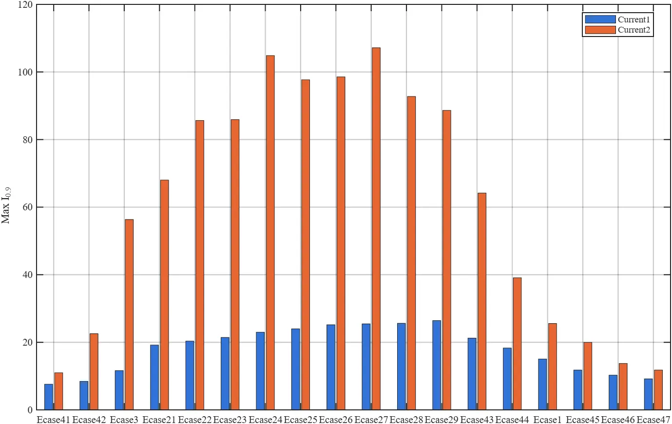
Table 11. ALS code check.
|
MBL |
$$\boldsymbol{T_D}$$ |
Result |
|
|---|---|---|---|
|
Light chain (Grade 3) |
3687.94 |
30 |
−187.65 < 0 |
|
24 |
26.22 > 0 |
||
|
Polyester |
2880.89 |
- |
161.35 > 0 |
|
Nylon |
2731.41 |
- |
11.87 > 0 |
In case of FLS check, the design inequality is defined in chapter 2 section 2 (6.4.1) of the DNVGL-OS-E301 (Edition July 2018) [33]:
|
```latex1-{d}_{c}\cdot {\gamma }_{F}\ge 0``` |
(10) |
Here $${d}_{c}$$ is the total fatigue damage accumulated throughout the lifespan. $${\gamma }_{F}$$ is the single safety factor. In this study, the fatigue damage was calculated by an integration of the T-N curve method, rain-flow analysis and Palmgren-Miner rule, based on the 3 h time-domain simulations of operational sea states mentioned in Table 4. According to chapter 2 section 2 (6.4.2) of the DNV standard [33], the chain’s safety factor $${\gamma }_{F}=5\sim8$$ is recommended. This safety factor is quite large due to the uncertainty of its recommended methods, such as the combined spectrum approach and the dual narrow-band approach. Considering that the rain-flow counting technique provides the most accurate estimate, a lower safety factor is reasonable. Thus, $${\gamma }_{F}=5$$ was adopted in this FLS code check, it is also used in recent works [35].
The fatigue damage was calculated by the T-N Curve formulated in OrcaFlex, defined by:
|
```latex\mathrm{N}={k\left(\frac{T}{RBS}\right)}^{-m}``` |
(11) |
Here $$T$$ and $$\mathrm{N}$$ represent the effective tension range and its corresponding cycles $$\mathrm{N}$$ to fatigue failure. $$k$$ and $$m$$ are constant values and related to the component’s type, for example, studless chain ($$m=3, k=316$$), studlink chain ($$m=3, k=1000$$), and polyester ($$m=13.46, k=0.259$$). $$RBS$$ represents reference breaking strength. For nylon and polyester ropes, no additional degradation factor is applied in this study, since the fibre rope segments are assumed to be intact and protected from severe abrasion or local damage. Accordingly, the RBS of the elastic ropes is taken as equal to their nominal MBL. As for the chain, a corrosion allowance is required. In chapter 2 section 2 (6.3.2) of the DNVGL-OS-E301 (Edition July 2018) [33], 50% of the chain corrosion allowance should be taken into account in FLS. Therefore, the corresponding RBS can be derived as:
|
```latexRBS\approx MBL\cdot {\left(\frac{{D}_{new}-0.5{r}_{corr}{T}_{D}}{{D}_{new}}\right)}^{2}``` |
(12) |
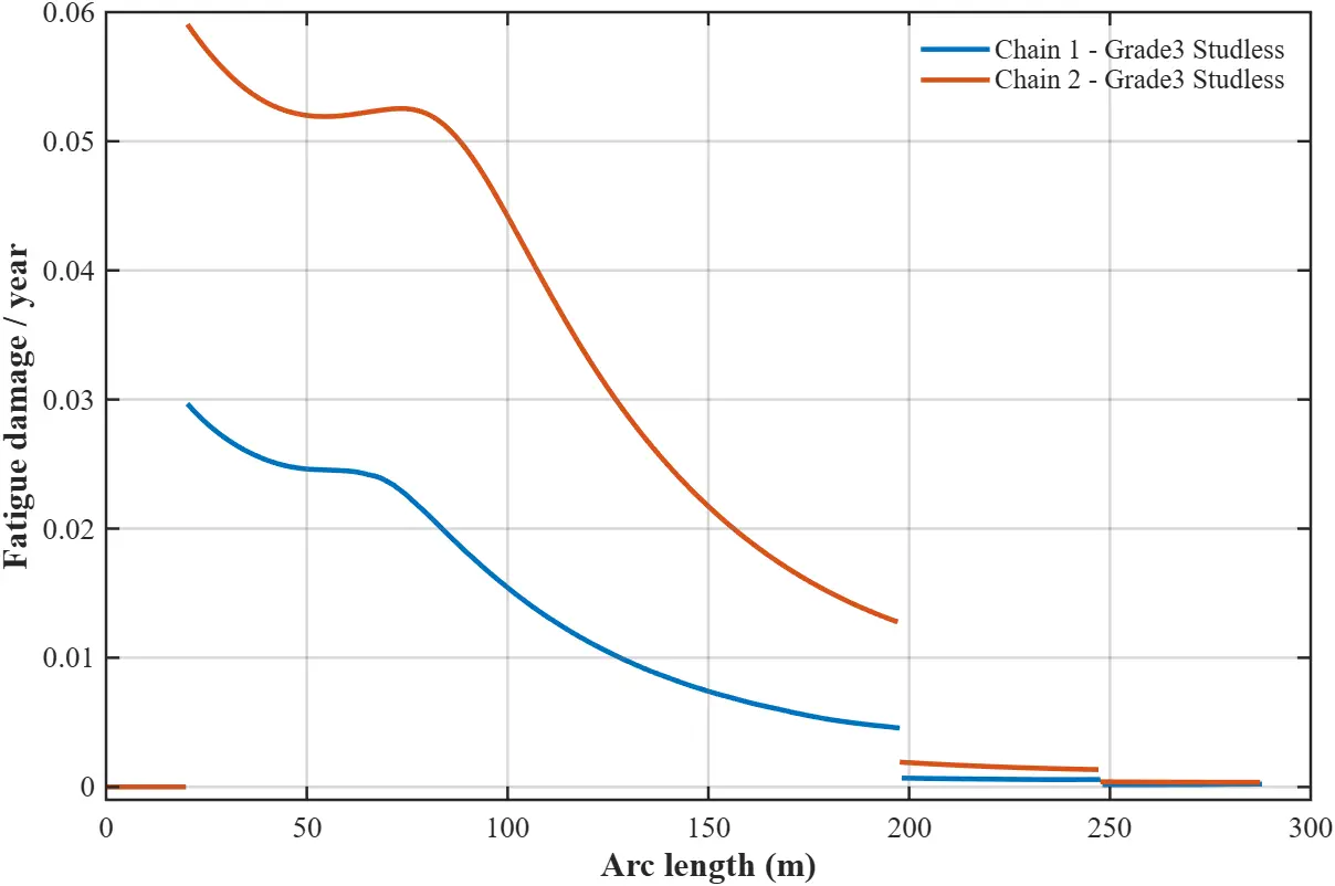
The annual bare fatigue damage without corrosion allowance, calculated by OrcaFlex, is shown in Figure 25. Here, Line3 is neglected as it shares the same result as Line2 when ignoring the misalignment of current and wave. The slope variation in arclength 50~100 m indicates the influence of touch down point. These curves illustrate that the light chains in Line2 and Line3 are prone to fatigue failure, and the max fatigue damage happens on the upper end of the light chain. The actual total fatigue damage $${d}_{c}$$ should include the corrosion deterioration and the design service life, the expression is given by:
|
```latex{d}_{c}={T}_{D}\cdot {d}_{c\_1y}\cdot {\left(\frac{MBL}{RBS}\right)}^{m}``` |
(13) |
Here, $${d}_{c\_1y}$$ denotes the annual bare fatigue damage.
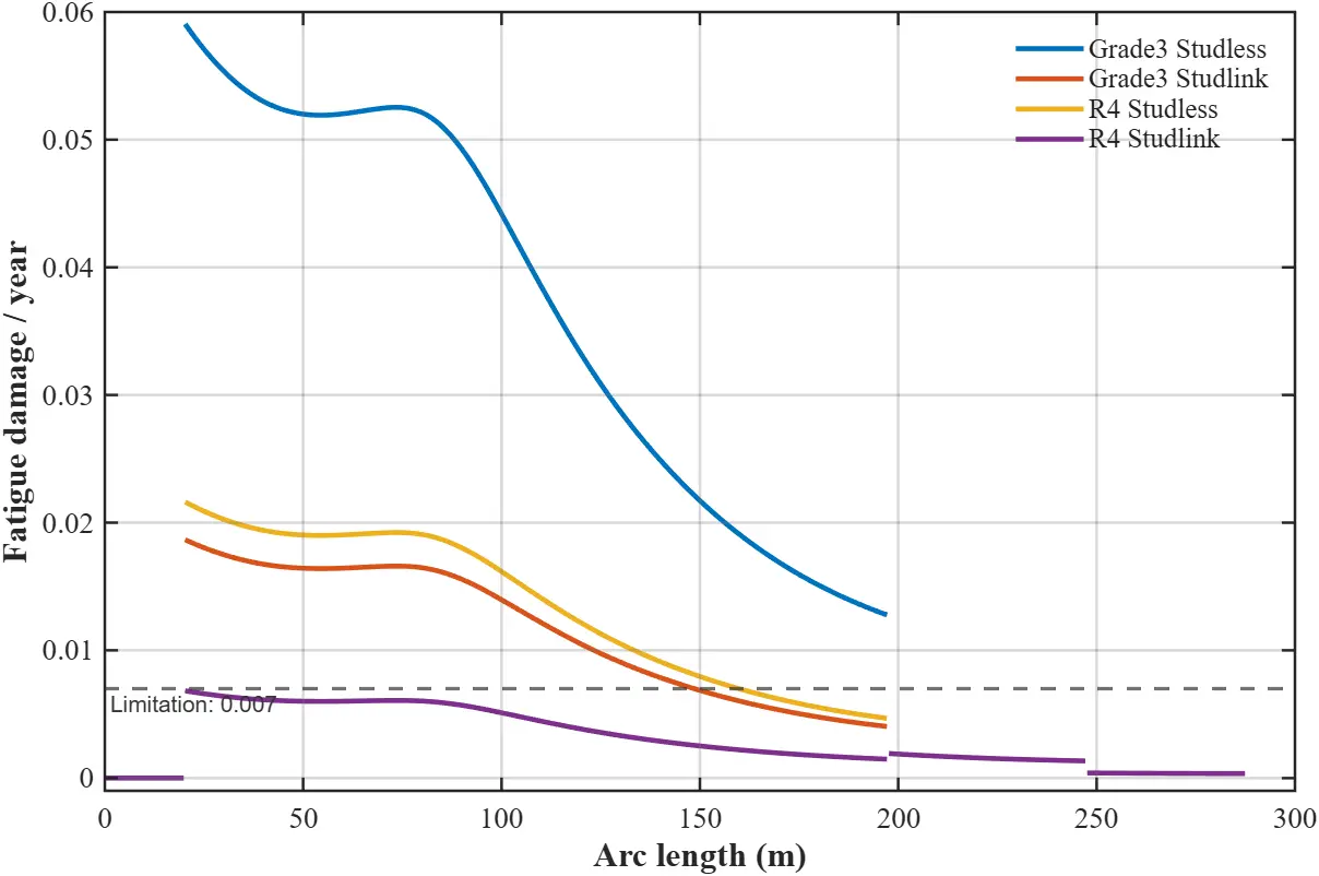
For this studless chain in Grade 3 strength, the maximum annual bare fatigue damage of 0.0591 is too high to ensure a long-term service life. Increasing the strength level or switching the type from studless to studlink can reduce fatigue damage. Therefore, different enhancements were proposed and compared in Figure 26. Here, the gray dashed line represents the equivalent annual bare damage $${d}_{cpt\_1y}$$ of the light chain, considering the corrosion allowance of service life $${T}_{D}=20$$ and the safety factor $${\gamma }_{F}=5$$. The definition of $${d}_{cpt\_1y}$$ is derived from Equation (13) and the assumption of $${d}_{c}\cdot {\gamma }_{F}=1$$:
|
```latex{\gamma }_{F}\cdot {T}_{D}\cdot {d}_{cpt\_1y}\cdot {\left(\frac{MBL}{RBS}\right)}^{m}=1``` |
(14) |
Specifically, $${d}_{cpt\_1y}$$ represents the upper limitation of annual bare fatigue damage for the chain with at least $${T}_{D}$$ years of design life, considering the corrosion influence and the safety factor. According to Figure 26, the studless light chain currently used in Line2,3 with Grade3 strength level obviously does not meet the 20-year fatigue design life, unless its type is switched from studless to studlink and the strength level is increased to R4. Thus, the light chain is replaced with this solution, though the results also illustrate that the couple of “Grade3 + Studlink” or “R4 + Studless” can be partly satisfied.
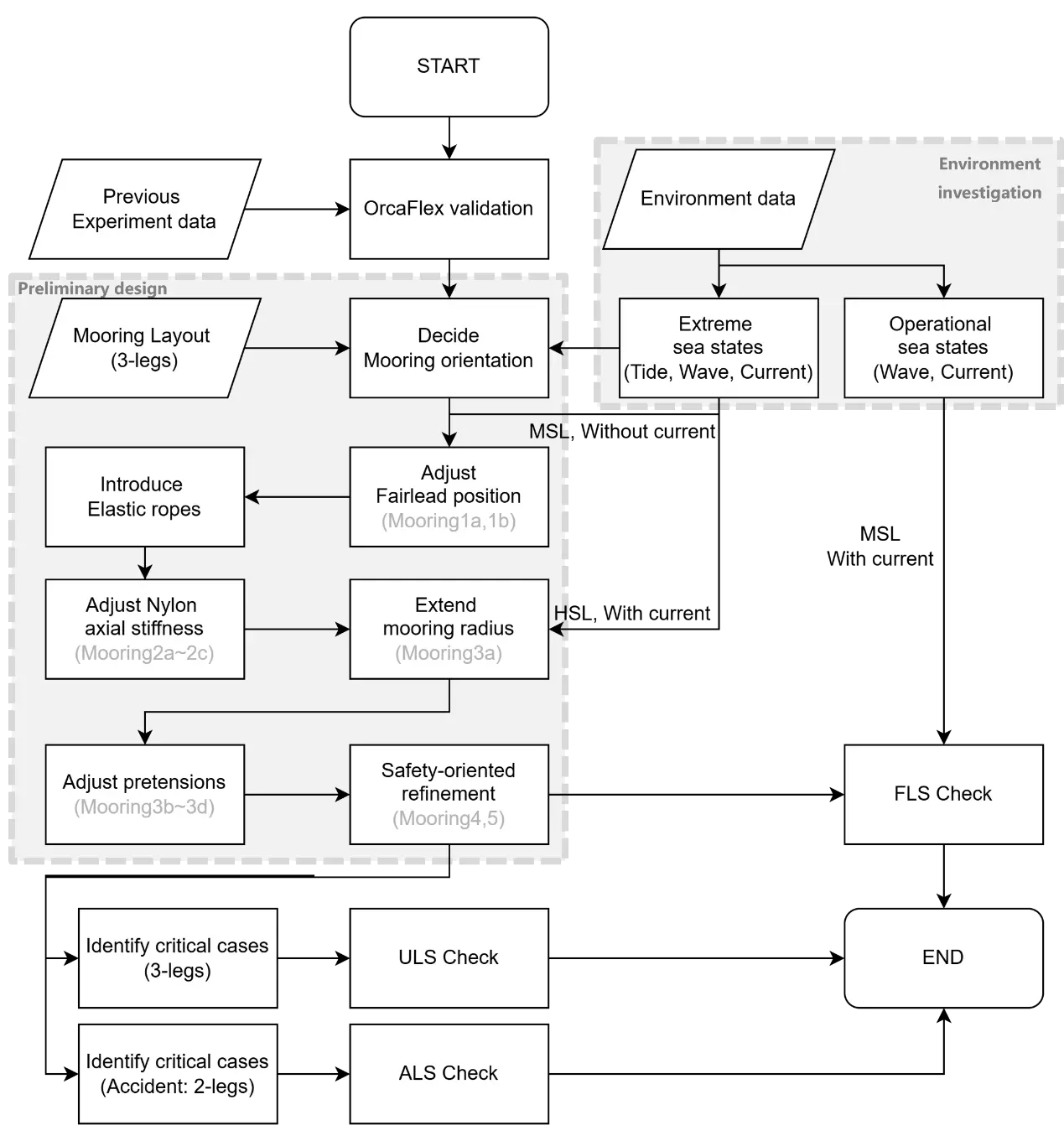
The flowchart of the whole mooring design process is shown in Figure 27.
3. Results and Discussions
3.1. Mooring Design Summary
According to the FLS code check, the Grade 3 studless light chain was replaced with a heavier studlink type with an R4 strength level. This adjustment can slightly reduce the snap load due to the increased weight; therefore, we are not worried about potential ULS/ALS variations of the elastic ropes. As for the light chain, it will definitely be safer because the MBL is increased.
The optimized design of the mooring line is detailed in Table 12. This hybrid mooring line begins with a segment of polyester connected to the WEC’s fairlead, which has good resistance against fatigue damage. The following nylon line features good elasticity and is utilized to effectively reduce potential snap loads. Then the light chain with the longest length along the line functions as the catenary to provide the majority of horizontal constraints. Its lengths on the bow side and stern side are slightly different in order to balance horizontal stiffness and reduce extreme offsets. The last two segments of the heavy chain behind are designed as a safety redundancy for extreme sea states. When a large offset occurs, these heavy components provide steeper horizontal stiffness to protect the anchor from direct impact caused by insufficient on-bottom length. Additionally, it is easier to control the mooring radius.
It is noted that these components should be connected to each other by shackles; however, this study does not provide a detailed discussion of them, as they are not the primary focus of this work.
Table 12. Line components and parameters of final design.
|
Component |
Properties |
MBL (kN) |
Diameter (mm) |
Length (m) |
Comment |
|---|---|---|---|---|---|
|
Polyester |
8-strand Multiplait |
2880.89 |
130 |
10 |
Top end connected to the fairlead; |
|
Nylon |
8-strand Multiplait |
2731.41 (wet) |
140 |
10 |
Nonlinear axial stiffness: Nylon31 |
|
Light chain |
Studlink, R4 |
5155.58 |
70 |
177.9 (Stern) 177.4 (Bow) |
Bow-side lines are shorter than that in stern-side; |
|
Heavy chain1 |
Studlink, Grade3 |
4716.54 |
80 |
50 |
\ |
|
Heavy chain2 |
Studlink, Grade3 |
7056.00 |
100 |
40 |
Bottom end linked with drag anchor or gravity anchor |
3.2. Mooring Performance Analysis
To further analyze the performance of this mooring design, a preliminary comparison with the original 4-leg mooring system in terms of energy production was conducted. Considering that the original 4-leg mooring system is unlikely to survive in extreme waves, an operational sea state (Ocase5 in Table 4) was selected as the incident wave with the closest Tp to the WEC’s pitch natural period. The horizontal pendulum was added to the numerical models for production evaluation, and its parameters are listed in Table 13. Here, the height of the pendulum is related to the buoy’s center of mass, and the length represents the distance from the rotational axis to the pendulum’s center of mass.
Table 13. Parameters of pendulum.
|
Mass |
Height |
Length |
Linear Damping |
|---|---|---|---|
|
15.4 te |
2.5 m |
1.3 m |
0.0226 kN·m·s/deg |
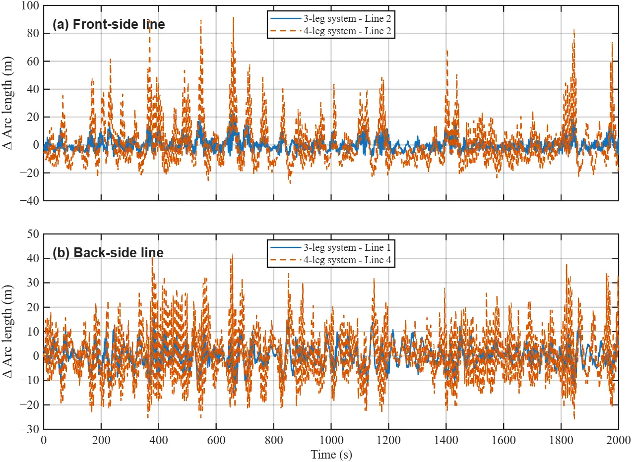
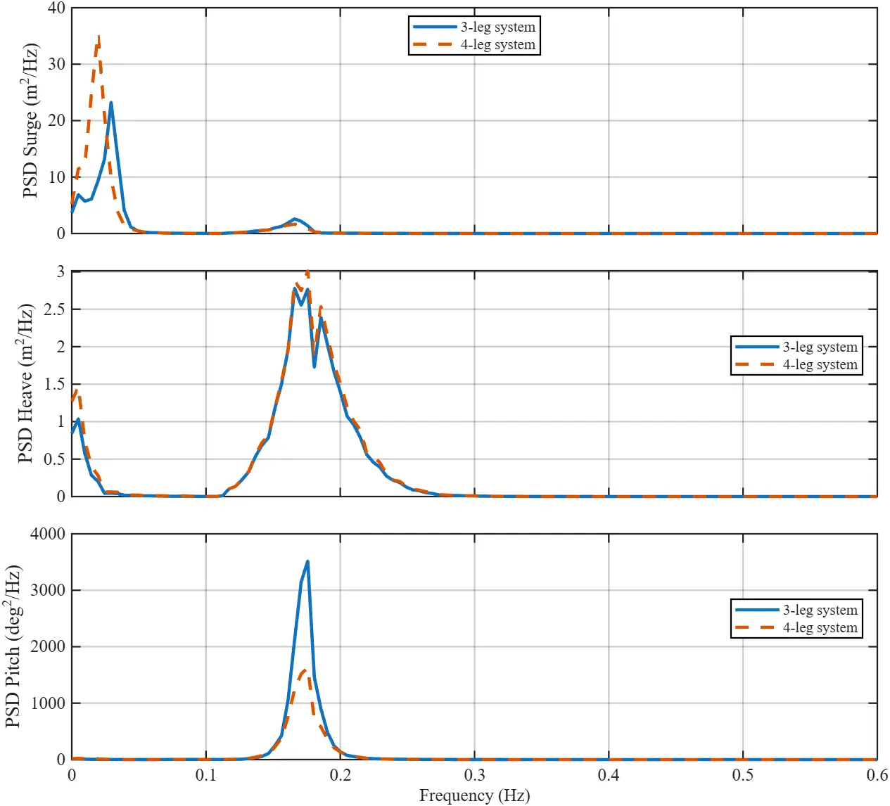
The peak tension distributions of the two moorings are compared in Figure 28, which indicates a similar level of maximum tension, while the redesigned 3-leg system has significantly smaller tension fluctuation. This change is meaningful due to its increasing stability and predictability of tension, together with lower potential fatigue damage. When it comes to the touchdown-point displacement as shown in Figure 29, a significant reduction is observed, indicating a drop in potential seabed-induced abrasion. These enhancements are mainly attributed to the increased pretension and the higher fairlead position, which reduce excitation from the buoy to the mooring lines.
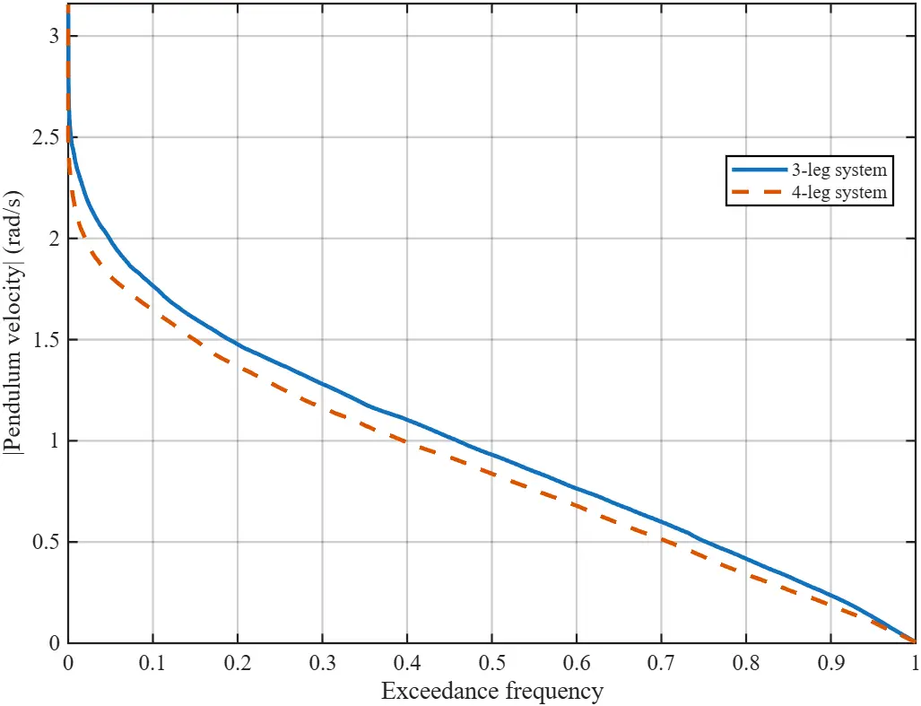
As for the production comparison, the Cumulative Frequency of the pendulum’s Angular Velocity (CFAV) [24] is compared in Figure 30. The pendulum exhibits greater response in the 3-leg hybrid mooring and results in a 20.7% increase in power production, which can be attributed to the enhanced pitch response as shown in Figure 31. Note that in this study, the pendulum installation position as well as PTO damping are not at optimal values as they are not the focus of this work. Therefore, the enhancement from the new mooring may be higher if the pendulum is properly optimized.
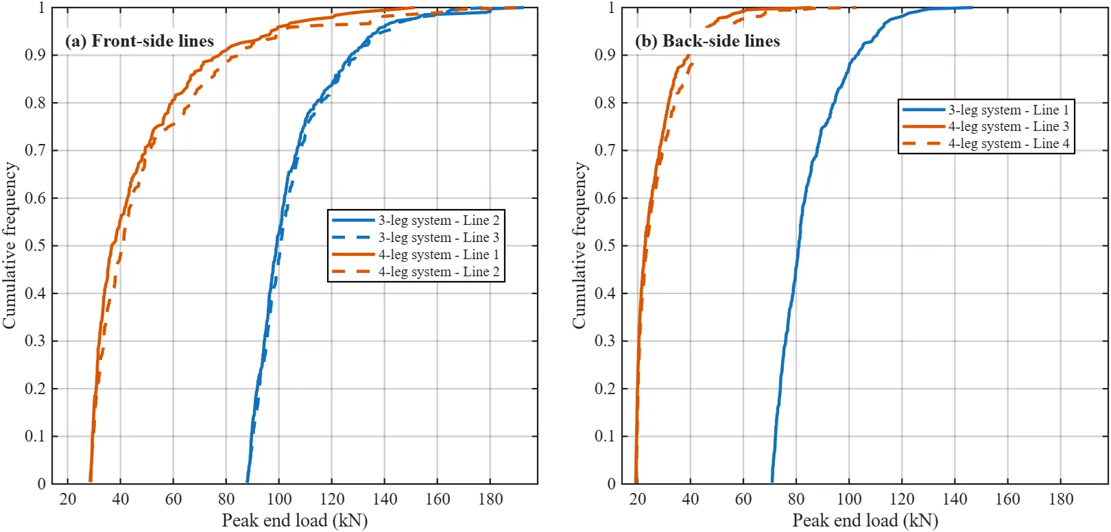
Figure 28. Comparison of tension peaks CDF (top end) between Designed mooring (3-leg) and Original mooring (4-leg): (a) Front-side line; (b) Back-side line.
3.3. Discussions
The designed mooring system for the pendulum-based WEC demonstrates many enhancements in both survivability and power production compared to the original 4-leg mooring system. It is obtained from a comprehensive design flow and step-by-step optimizations. Within this design process, some noteworthy results are obtained.
The fairlead comparison illustrates that lower extreme load and larger pitch motion can be achieved simultaneously, indicating the importance of fairlead optimization in the WEC relying on pitch motion. Furthermore, the adoption of nylon ropes significantly reduces the tension in extreme sea states, and the polyester near the fairlead performs good resistance against fatigue damage. However, the nonlinear axial stiffness may result in higher tension than that in linear assumptions through the comparison. Therefore, it is better to consider nylon axial stiffness in nonlinear to avoid tension underestimation. Also, the increasement of nylon strength should be carefully considered because it may deteriorate the performance in snap load reduction.
The extreme sea state comparisons demonstrate the currents’ significant influence on the tension load, indicating that including current weighting in mooring orientation design may further reduce extreme tension. As for the accidental sea state as shown in Figure 23, once the single-line failure happens, the power cable will definitely be destroyed due to the extremely high offsets.
The code check in FLS reveals a significantly smaller design life than that in ULS/ALS, indicating the dominant role of fatigue damage in mooring safety, especially for WEC devices with large response amplitude and high-tension range. Therefore, in the preliminary design process, more attention should be paid to the variations of the tension range when adjusting mooring parameters. This may avoid the undesired design with high service life in ULS while significantly low design life in FLS.
It is noted that our mooring design is conservative due to two reasons: (1) the designed current speed is relatively high because the joint distribution of wave and current is not considered. (2) Current load coefficients specified in the numerical model are 0.8, which is relatively high. Usually, a value of 0.5~0.8 is acceptable.
4. Conclusions
This study provides a comprehensive mooring design flow for the pendulum-based WEC, starting from the environmental investigation, to a step-by-step preliminary design, and finally ends with a detailed safety code check on ULS, ALS, and FLS. The numerical model agrees well with the experimental data, which demonstrates its ability for precise evaluation and its competence as a design tool. Through a series of design and optimization, a 3-leg hybrid mooring system with redundancy and improved production is finally proposed.
The designed mooring system is compared with the original 4-leg catenaries and demonstrates significant enhancements in safety and performance, with an increase in production of at least 20.7%. These improvements are mainly attributed to the pretension and fairlead adjustments. It is noted that a proper fairlead position design can not only improve tension patterns but also benefit WEC pitch response. Furthermore, according to the code check, the results indicate that FLS becomes the governing design consideration for moored WECs, and thus should receive greater attention to prevent an excessive discrepancy between the design lives associated with ULS and FLS.
Future work can consider the following topics: (1) Pendulum’s influence on mooring lines design. (2) Detailed fairlead position optimization and its influence on extreme tension as well as fatigue damage. (3) Developing a simplified fatigue calculation approach for the preliminary mooring design stage, for example, predicting line tension series through a surrogate model based on machine learning or a nonlinear interpolation algorithm.
Statement of the Use of Generative AI and AI-Assisted Technologies in the Writing Process
During the preparation of this manuscript, the authors used Grammarly to check grammar and improve the language and readability of the manuscript. After using this tool, the authors reviewed and edited the content as needed and take full responsibility for the content of the published article.
Acknowledgments
The authors would like to acknowledge support from the China Scholarship Council and the University of Plymouth for the OcEn funding support.
Author Contributions
Conceptualization, X.J., C.Z. and L.J.; Methodology, X.J. and C.Z.; Validation, X.J.; Formal Analysis, X.J. and C.Z.; Investigation, X.J.; Resources, H.S. and L.J.; Data Curation, X.J.; Writing—Original Draft Preparation, X.J.; Writing—Review & Editing, C.Z., H.S. and L.J.; Visualization, X.J.; Supervision, C.Z., H.S. and L.J.
Ethics Statement
Not applicable.
Informed Consent Statement
Not applicable.
Data Availability Statement
The data presented in this study are available from the corresponding author upon reasonable request.
Funding
X.J. was supported by the China Scholarship Council through a scholarship for living expenses (Grant No. 202406330114). The article processing charge (APC) was waived by the publisher.
Declaration of Competing Interests
Author L.J. serves as an Executive Editor-in-Chief of this journal. L.J. was not involved in the editorial handling, peer-review process, or decision-making for this manuscript. The remaining authors declare no competing interests.
References
- Moura Paredes G, Eskilsson C, Engsig-Karup AP. Uncertainty Quantification in Mooring Cable Dynamics Using Polynomial Chaos Expansions. J. Mar. Sci. Eng. 2020, 8, 162. DOI:10.3390/jmse8030162 [Google Scholar]
- Thomsen J, Ferri F, Kofoed J, Black K. Cost Optimization of Mooring Solutions for Large Floating Wave Energy Converters. Energies 2018, 11, 159. DOI:10.3390/en11010159 [Google Scholar]
- Martinelli L, Zanuttigh B. Effects of Mooring Compliancy on the Mooring Forces, Power Production, and Dynamics of a Floating Wave Activated Body Energy Converter. Energies 2018, 11, 3535. DOI:10.3390/en11123535 [Google Scholar]
- Qiao D, Haider R, Yan J, Ning D, Li B. Review of Wave Energy Converter and Design of Mooring System. Sustainability 2020, 12, 8251. DOI:10.3390/su12198251 [Google Scholar]
- Lee CF, Fjermedal S, Ong MC. Design and analysis of taut mooring systems for a combined floating offshore wind and wave energy system at intermediate water depth. Ocean Eng. 2024, 312, 119174. DOI:10.1016/j.oceaneng.2024.119174 [Google Scholar]
- Xu S, Wang S, Guedes Soares C. Review of mooring design for floating wave energy converters. Renew. Sustain. Energy Rev. 2019, 111, 595–621. DOI:10.1016/j.rser.2019.05.027 [Google Scholar]
- Zhao J, Bian S, Liu Z, Lin X. Polyester mooring system design and evaluation of a semi-platform in south China sea. Mar. Struct. 2025, 99, 103686. DOI:10.1016/j.marstruc.2024.103686 [Google Scholar]
- Ridge IML, Banfield SJ, Mackay J. Nylon fibre rope moorings for wave energy converters. In Proceedings of the OCEANS 2010 MTS/IEEE SEATTLE, Seattle, WA, USA, 20–23 September 2010; pp. 1–10. DOI:10.1109/OCEANS.2010.5663836 [Google Scholar]
- Housner S, Hall M, Tran TT, de Miguel Para B, Maeso A. Shared mooring system designs and cost estimates for wave energy arrays. Renew. Energy 2024, 231, 120924. DOI:10.1016/j.renene.2024.120924 [Google Scholar]
- Howey B, Collins KM, Hann M, Iglesias G, Gomes RPF, Henriques JCC, et al. Compact floating wave energy converter arrays: Inter-device mooring connectivity and performance. Appl. Ocean Res. 2021, 115, 102820. DOI:10.1016/j.apor.2021.102820 [Google Scholar]
- Ning D, Wang S, Chen H, Guedes Soares C. Coupled dynamics of a point absorber array with a shared mooring system. Ocean Eng. 2026, 343, 123447. DOI:10.1016/j.oceaneng.2025.123447 [Google Scholar]
- Davidson J, Ringwood J. Mathematical Modelling of Mooring Systems for Wave Energy Converters—A Review. Energies 2017, 10, 666. DOI:10.3390/en10050666 [Google Scholar]
- Zhong W, Zhao W, Wan D, Zhao Y. Comparison study on mooring line models for hydrodynamic performances of floating offshore wind turbines. Ocean Eng. 2024, 296, 117083. DOI:10.1016/j.oceaneng.2024.117083 [Google Scholar]
- Cordonnier J, Gorintin F, De Cagny A, Clément AH, Babarit A. SEAREV: Case study of the development of a wave energy converter. Renew. Energy 2015, 80, 40–52. DOI:10.1016/j.renene.2015.01.061 [Google Scholar]
- Sirigu SA, Bonfanti M, Begovic E, Bertorello C, Dafnakis P, Giorgi G, et al. Experimental Investigation of the Mooring System of a Wave Energy Converter in Operating and Extreme Wave Conditions. J. Mar. Sci. Eng. 2020, 8, 180. DOI:10.3390/jmse8030180 [Google Scholar]
- Paduano B, Pasta E, Papini G, Carapellese F, Bracco G. Mooring Influence on the Productivity of a Pitching Wave Energy Converter. In Proceedings of the OCEANS 2021: San Diego–Porto, San Diego, CA, USA, 20–23 September 2021; pp. 1–6. DOI:10.23919/OCEANS44145.2021.9706108 [Google Scholar]
- Cervelli G, Battisti B, Mattiazzo G. On the influence of multidirectional irregular waves on the PeWEC device. Front. Energy Res. 2022, 10, 908529. DOI:10.3389/fenrg.2022.908529 [Google Scholar]
- Xue G, Qin J, Zhang Z, Huang S, Liu Y. Experimental Investigation of Mooring Performance and Energy-Harvesting Performance of Eccentric Rotor Wave Energy Converter. J. Mar. Sci. Eng. 2022, 10, 1774. DOI:10.3390/jmse10111774 [Google Scholar]
- Xue G, Liu Y, Huang S, Xue Y, Qin J, Zhang Z. Effect of mooring mode and internal mass block layout on eccentric rotating wave energy converter model. Proc. Inst. Mech. Eng. Part A J. Power Energy 2022, 236, 1370–1388. DOI:10.1177/09576509221092286 [Google Scholar]
- Depalo F, Wang S, Xu S, Guedes Soares C. Design and Analysis of a Mooring System for a Wave Energy Converter. J. Mar. Sci. Eng. 2021, 9, 782. DOI:10.3390/jmse9070782 [Google Scholar]
- Zhao C, Khalid F, Lewis T, Barrett S, McSwiney B, Pascal RC, et al. Advancements in mooring systems for the OE35 wave energy converter: Dynamic design and validation. Ocean Eng. 2025, 330, 121235. DOI:10.1016/j.oceaneng.2025.121235 [Google Scholar]
- Cerveira F, Fonseca N, Pascoal R. Mooring system influence on the efficiency of wave energy converters. Int. J. Mar. Energy 2013, 3–4, 65–81. DOI:10.1016/j.ijome.2013.11.006 [Google Scholar]
- Jiang X, Cao F, Shi H, Zhu K, Zhang C. Optimization of pendulum-based wave energy converter through mathematical approximation. Appl. Energy 2025, 378, 124754. DOI:10.1016/j.apenergy.2024.124754 [Google Scholar]
- Jiang X, Shi H, Cao F, Zhao Z, Li M, Chen Z. System analysis and experimental investigation of a pendulum-based wave energy converter. Ocean Eng. 2023, 277, 114300. DOI:10.1016/j.oceaneng.2023.114300 [Google Scholar]
- Orcina. Orcaflex. Available online: https://www.orcina.com/orcaflex/ (accessed on 27 April 2026).
- Sun P, Xu B, Wang J. Long-term trend analysis and wave energy assessment based on ERA5 wave reanalysis along the Chinese coastline. Appl. Energy 2022, 324, 119709. DOI:10.1016/j.apenergy.2022.119709 [Google Scholar]
- Pastor J, Liu Y. Wave Climate Resource Analysis Based on a Revised Gamma Spectrum for Wave Energy Conversion Technology. Sustainability 2016, 8, 1321. DOI:10.3390/su8121321 [Google Scholar]
- Ma KT, Luo Y, Kwan T, Wu Y. Mooring analysis. In Mooring System Engineering for Offshore Structures; Elsevier: Amsterdam, The Netherlands, 2019; pp. 85–114. DOI:10.1016/B978-0-12-818551-3.00005-3 [Google Scholar]
- European Union-Copernicus Marine Service. Global Total (COPERNICUS-GLOBCURRENT), Ekman and Geostrophic Currents at the Surface and 15m; Mercator Ocean International: Toulouse, France, 2023. DOI:10.48670/MDS-00327 [Google Scholar]
- European Union-Copernicus Marine Service. Global Ocean Waves Reanalysis WAVERYS; Mercator Ocean International: Toulouse, France, 2019. DOI:10.48670/MOI-00022 [Google Scholar]
- Copernicus Climate Change Service. Global Sea Level Change Time Series from 1950 to 2050 Derived from Reanalysis and High Resolution CMIP6 Climate Projections; ECMWF: Reading, UK, 2022. DOI:10.24381/CDS.A6D42D60 [Google Scholar]
- Mackay E, de Hauteclocque G. Model-free environmental contours in higher dimensions. Ocean Eng. 2023, 273, 113959. DOI:10.1016/j.oceaneng.2023.113959 [Google Scholar]
- DNVGL-OS-E301; Position Mooring. DNV GL AS: Høvik, Norway, 2018. [Google Scholar]
- Barrera C, Guanche R, Losada IJ. Experimental modelling of mooring systems for floating marine energy concepts. Mar. Struct. 2019, 63, 153–180. DOI:10.1016/j.marstruc.2018.08.003 [Google Scholar]
- Gao X, Liu X, Xue X, Chen NZ. Fracture mechanics-based mooring system fatigue analysis for a spar-based floating offshore wind turbine. Ocean Eng. 2021, 223, 108618. DOI:10.1016/j.oceaneng.2021.108618 [Google Scholar]