
A Framework for Quantifying Autonomy in Robotic Systems
A Framework for Quantifying Autonomy in Robotic Systems
Received: 11 April 2026 Revised: 12 June 2026 Accepted: 22 June 2026 Published: 28 July 2026

© 2026 The authors. This is an open access article under the Creative Commons Attribution 4.0 International License (https://creativecommons.org/licenses/by/4.0/).
1. Introduction
Humans have been the main higher-level controllers for most complex robotic systems due to their perceptual, manipulation, decision-making, problem-solving and other cognitive and physical abilities. However, robotic systems are finding applications in partially observable, highly uncertain, and highly dynamic environments whose control requirements exceed human regulation capability. Therefore, system stability under exclusive human control for such applications cannot be guaranteed. Furthermore, human control integrity fluctuates, leading to poor decisions and slow responses that sometimes result in accidents. This phenomenon is known as human error and is responsible for 94 ± 2.2% of road vehicle crashes [1] and 80% of civil aviation accidents [2]. These together call for the integration of machine-based control and decision-making to enable autonomous system performance. In such settings, assessing autonomous performance is crucial and cannot rely solely on whether a robot completes a task, because two robots may both succeed while differing substantially in safety, robustness, efficiency, and reliability. A robot that frequently approaches obstacles, executes energy-inefficient trajectories, or fails under rare conditions can appear effective in small-scale demonstrations but may be unsuitable for real-world operation. Conversely, overly conservative behavior may maximize safety while sacrificing productivity. Therefore, autonomy evaluation requires performance measures that are quantitative, comparable across systems, and interpretable in terms of underlying robot capabilities. Additionally, they should be easily measurable, sensitive to performance differences, extensive enough to capture the evolution of autonomy in a system, amenable to quantitative analysis, and have good output resolution.
In this work, we propose a set of quantitative autonomy metrics derived from a relationship between robot task characteristics and the human job characteristics applied in industries. We recognized that autonomous capability is designed for a specific task or to demonstrate an emergent behavior, and is associated with a predefined set of performance requirements. Autonomy is therefore task-oriented and operating domain-specific. Since performance requirements change as new environments and applications emerge, a good autonomy assessment framework must be sensitive to these changes. Such a framework based on system capability and performance thereof is presented herein and its details described in the following sections: Section 2 puts this work in context with the existing related literature; Section 3 gives a detailed description of the proposed metrics, their associated mathematical definitions, and level of autonomy and degree of autonomy mathematical models; Section 4 describes the integrity monitoring process integrated into the framework; Section 5 provides application demonstrations for the proposed autonomy framework; Section 6 presents the concluding remarks.
The framework supports not only quantitative assessment of autonomy, but also integrity monitoring when implemented online. The former affords mathematical analysis, whereas the latter is key in ensuring safety in complex dynamic systems like drones and medical robots. Furthermore, the fact that capability performance is evaluated with respect to reference performance requirements is expected to boost human trust in autonomous systems as well as simplify the processes of their design and regulation.
2. Background and Related Work
Factors motivating the increasing demand for autonomous systems include the need of replacing human operators [3] safety risk assessment, handling of complex applications and attaining time critical responses [4], operating domain qualification and delineation [5], basis for control architecture selection [6], characterization of autonomous technologies and assessing technology maturity [7], operator training and licensing [8], and reducing operating costs whilst maximizing mission success [9], among others. However, the resulting global surge in their development and deployment has inadvertently raised regulatory, safety, and ethical concerns. Although proper regulatory laws and good engineering practices can address these concerns, their formulation requires tools and metrics for quantifying autonomy.
The existing autonomy assessment techniques can be categorized based on the choice of metrics or on the nature of their outputs. The former category is the most prevalent in the literature, with representative examples including the bandwidth approach in [4] which viewed autonomy as a measure of supervision, parameterized by the data transmission rate between the external controller and the system. Although simple, the metric assumed commands to have equal importance to the fulfillment of the task, which is generally true only for very simple tasks. Additionally, the entropy of each command and the knowledge representation may differ, resulting in varying amounts of information per command. The ALFUS workgroup of NIST (National Institute of Standards and Technology) extended this view to two measures, namely autonomy and level of autonomy. The former is a function of task complexity, degree of operator independence, and environment complexity, while the latter is a measure of the degree of operator independence [10]. Unfortunately, their proposed metrics are subjective and lack quantitative interpretations needed in order to support mathematical analysis.
Autonomy as measured by the degree of supervision, is not applicable to fully autonomous systems. To overcome this, the assessment technique presented in [5] defined autonomy as a measure of performance parameterized by two metrics, namely environment complexity and information quality. But as noted before, information quality is not only a bad metric for fully autonomous systems, but also oblivious to the actual performance of the underlying capability.
The output formats in literature include ordinal, ratio, and interval measurements [8]. The ordinal-scale frameworks divide autonomy into discrete levels. A common example is the ACL (Autonomy Control Level) chart in [3]. It has eleven levels, numbered zero to ten, with zero representing remotely operated systems, ten representing fully autonomous systems, and levels in-between representing a monotonic increase in autonomous capability. To specify a system’s level, four metrics, including perception, analysis, decision making, and ability, were applied. These were adopted from the OODA (Observe, Orient, Decide, Act) loop. A similar eleven level chart was proposed in [10], but with levels assigned based on operator independence. The authors extended their framework to include task complexity and environment complexity metrics, which promoted the output format to a ratio-scale measure. A similar trend has been witnessed in the automotive industry, where the SAE’s levels of driving automation [11] chart proved insufficient for autonomous performance assessment, motivating the department of motor vehicles of the state of California to devise a ratio-scale measure based on the disengagement rate metric [12]. But this online metric is also incapable of capturing performance nuances of a driving system, i.e., it does not account for environment complexity, system integrity and availability, or driving quality. Worst of all, one can strategically select test routes, time of day, duration, and/or weather conditions to minimize disengagement rate, rendering it a bad measure according to Goodhart’s law [13]. Other works with ratio-scale output formats include [6,14,15]. In Ref. [6], the authors premised that autonomous systems have an automated problem-solving process and measured autonomy as levels of automation of the problem-solving process using either Equation (1), where $$n$$ is the number of autonomous capabilities considered, and $${\delta }_{D}$$, $${\delta }_{E}$$, $${\delta }_{S}$$, $${\delta }_{I}$$ and $${\delta }_{V}$$ are levels of automation for definition, exploration, selection, implementation, and verification capabilities, respectively, or Equation (2), where $$\eta$$ quotients are ratios of actual (act) to standard (std) system behavior for definition ($$D$$), exploration $$\left(E\right)$$, selection $$\left(S\right)$$, implementation $$\left(I\right)$$ and verification $$\left(V\right)$$ capabilities.
As such, it is limited to scripted or deterministic behaviors. The research work in [14] defined autonomy as a measure of human effort expressed by Equation (3), where $$F$$, $$p$$, $$a$$ and $$t$$ are human effort, performance, area and time, respectively, whereas that in [15] defined it as a measure of information and formulated it as Equation (4), where $${B}_{C}$$, $${B}_{T}$$, $${T}_{C}$$, and $${T}_{T}$$, are control bits, total message size, contact time, and total mission time, respectively. The coefficient $${C}_{n}$$, and exponents $$i$$ and $$j$$ are constants that are determined empirically. But as already mentioned, information and the quality of operator inputs are not applicable to fully autonomous systems.
Autonomy can be achieved using deterministic or nondeterministic methods. By observation, both implementations are considered intelligent, i.e., extrinsic intelligence—exercising abilities considered intelligent when performed by humans [16]. In actuality, only nondeterministic methods yield intrinsic intelligence—systems built from intelligent building blocks. Extrinsic intelligence is incognizant of the underlying implementation, making it incapable of distinguishing automatic from autonomous functioning, and is not considered herein.
Batch testing of the frameworks presented in [3,7,10] and seven others on the classification of six unmanned aircraft systems revealed that only four frameworks were able to classify all six vehicles, but only one was able to unambiguously classify all six. Unfortunately, even the one that unambiguously classified all six failed to distinguish between a vehicle with unsupervised capabilities, a vehicle with supervised capabilities, and a purely remotely operated vehicle [8]. This highlighted a continued need for a better autonomy assessment technique.
Unlike the above reported approaches, which output either an ordinal or ratio-scale measure, the one presented herein outputs a hybrid measure consisting of an ordinal-scale measure known as LoA (Level of Autonomy) and its associated ratio-scale measure known as DoA (Degree of Autonomy). This hybridization stemmed from the realization that autonomous systems differ not only in their available capabilities (kind), but also in capability performance (degree). The framework applies multiple metrics, rendering it less susceptible to the Goodhart’s law. To assess LoA, the framework adopted the autonomy level chart representations of [3,10], but with custom level descriptions. More details on LoA and DoA are given in Section 3.2. In establishing autonomy metrics, works like [17] applied biomorphic survival laws, we derived ours from human job characteristics to reflect the task-oriented nature of robotic systems. This made sense since robots ultimately replace human skilled workers.
3. Autonomy Quantification
Quantifying autonomy requires the identification of appropriate metrics. But how does one identify such metrics? The search for metrics should focus on an impartial search space and steer away from particular biases and distinctive system features. Following these principles, the resulting metrics should be invariant to implementation choices, such as state estimators and sensor fusion methods, software architecture, computing architecture, and modeling strategy, to mention a few.
As autonomous systems ultimately replace human skilled workers, it was prudent to start by examining human-job characteristics applied in industries. This examination identified the four characteristics listed in the left column of Table 1, whereas in the right column are their translations to the robotics domain, and in the middle column are their relative weights adopted from [18]. The review of autonomy assessment criteria for marine systems in [6] indicated that 20% of the reviewed frameworks applied environment, task, behaviors, and interaction criteria, which pointed to the selected characteristics as having merit. This then constrained the metrics search to the four robot-task characteristics in Table 1.
Table 1. Human-job characteristics mapped to robot-task characteristics.
|
Human-Job Characteristics a |
Importance Weights |
Robot-Task Characteristics |
|---|---|---|
|
Skills and knowledge |
50% |
Capability |
|
Independence and responsibility |
25% |
Reliability |
|
Workload |
15% |
Responsiveness |
|
Workplace conditions |
10% |
Environment complexity |
|
Total |
100% |
a Column entries adopted from [18].
The robot-task characteristics in Table 1 emphasize that a task can be performed only if the robot has the necessary capabilities. To ensure some degree of safety and robustness, these capabilities should perform reliably and efficiently with respect to a given set of operating conditions.
Although a skilled human was taken as a reference in identifying the robot-task characteristics, the goal of developing autonomous systems with a capability set as diverse as that of a skilled human is one considered unnecessary since these systems are task-oriented and domain specific. Therefore, herein, autonomous functioning is limited to a specific task and operating domain.
3.1. Autonomy Metrics
As the desiderata for solving any task is the possession of all essential capabilities that meet the performance requirements of that task and its operating domain, the desired metrics should capture both the existence of essential capabilities as well as their performance. Herein, autonomy is considered as a measure of intelligence-guided performance, with performance parametrized by accuracy and rate of response. But since the ground-truth is usually unknown, it is not always possible to determine accuracy explicitly. We therefore opted for statistical error bounds and used variance instead of accuracy.
In addition to the actual variance and response rate of a capability, one also needs to know the required variance and response rate to be able to evaluate the suitability of the capability at a given task. Requirements are usually set by regulators, industrial benchmarks or system designers through application of the law of requisite variety (Equation (5)) to account for the complexity of both the task and the operating domain.
Then, the policy for acceptable autonomous functioning ability of a system becomes possession of all essential capabilities with variances and response rates that meet the performance requirements. Therefore, out of four robot-task characteristics, three metrics emerged, namely a requisite capability set, reliability, and responsiveness. The policy explicitly considers capability, reliability, and responsiveness characteristics, while implicitly accounts for the environmental complexity through requirement specifications.
3.1.1. Capability
Capability refers to the robot’s inherent skills, functionalities, or potential to perform certain tasks. Each capability is independent, corresponds to a specific function, is reusable across tasks, varies in performance, and has performance constraints. It encompasses the underlying technology, algorithms, and subsystems that enable behaviors. Therefore, capabilities are fixed by design and hardware, and they determine the tasks the robot can perform.
Transforming capabilities into an effective task-solving solution involves identifying the essential capabilities to accomplish the task, conducting a task analysis to determine their performance requirements and constraints, and developing systems to coordinate the capabilities. With the assumption of a capability-based paradigm, solving a task then becomes a matter of systematic coordination of capabilities. Therefore, one can rightly state that underlying any task-solving ability is a set of capabilities and a capability-coordination mechanism.
The concept of associating each human-job with a set of skills is extendable to robot tasks through the association of each robot-task with a set of essential capabilities. The associated set then becomes a tool for evaluating the feasibility of an autonomous system performing a specific task. To illustrate this, let $$R$$ be the set of essential capabilities for a specific task, and $$S$$ be the set of available capabilities of the robot. Then, a task is considered feasible if and only if $$R\subseteq S$$. As indicated in Table 2, different tasks utilize different sets of capabilities. We call these the requisite capabilities. Since a system may possess extra capabilities than those required for a particular task, the extras form the auxiliary capability set and are excluded from the evaluation.
Table 2. Autonomous mobile robotic applications and their capabilities.
|
Application |
Essential Capability |
Auxiliary Capability |
|---|---|---|
|
Search and rescue with: a single vehicle; multiple vehicles |
Localization, motion control, path following/trajectory tracking, object detection, motion planning, and communication for multiple vehicles |
Inter-vehicle coordination, object recognition |
|
Emergency response to: natural disasters; distress calls |
Localization, motion control, path following/trajectory tracking, communication, motion planning, object detection |
Inter-vehicle coordination, object recognition |
|
Remote sensing for: environmental monitoring; meteorology |
Localization, motion control, path/trajectory tracking, communication, motion planning, object detection |
Inter-vehicle coordination, object recognition |
|
Delivery service for: healthcare supplies; logistics; disaster relief |
Localization, motion control, path following/trajectory tracking, motion planning |
Communication, object detection, object recognition |
|
Wireless communication network with: a single vehicle; multiple vehicles |
Localization, motion control, path/trajectory tracking, motion planning, and communication for multiple vehicles |
Inter-vehicle coordination for multiple vehicles |
|
Inspection and surveillance of: coast lines; construction sites; infrastructure; irrigation channels; property; assets |
Localization, motion control, path following/trajectory tracking, communication, motion planning, object detection |
Object recognition, object tracking |
|
Real-time disaster monitoring for: forest fires; landslides; floods; avalanche; volcanic eruptions |
Localization, motion control, path following/trajectory tracking, communication, motion planning, object detection |
Object recognition, object tracking |
|
Photography and videography in: filming; journalism; photogrammetry; real-estate |
Localization, motion control, path following/trajectory tracking, communication, motion planning, object detection, object tracking |
Object recognition |
|
Mapping and survey for: archaeological documentation; urban planning; land use mapping; mining |
Localization, motion control, path following/trajectory tracking, mapping, communication, motion planning |
Object recognition, object detection |
|
Agriculture: crop sensing; pest control (spraying and dusting) |
Localization, motion control, coverage path following/trajectory tracking, motion planning, object detection |
Object recognition, communication |
|
Wildlife monitoring: tracking of poachers; animal census; animal behavior monitoring |
Localization, motion control, path following/trajectory tracking, communication, motion planning, object detection |
Object recognition, object tracking |
|
Law enforcement: surveillance and monitoring; tracking of subjects; public address system; forensics |
Localization, motion control, path following/trajectory tracking, object detection, communication |
Object recognition, object tracking |
|
Autonomous vehicles: urban driving, motorway driving, parking |
Localization, motion planning, motion control, path following, object detection, object tracking |
Communication, object recognition, adaptive learning |
Quantifying the performance of a capability is essential to knowing whether a robot can reliably perform specific tasks. This is achieved through the reliability and responsiveness metrics, which measure how well a capability works under given conditions.
3.1.2. Reliability Factor
Reliability evaluates the consistency of a capability’s performance under a given range of operating conditions. It indicates the likelihood of all errors falling within a predefined limit. The specific error limit depends on the parameters of the error model. Modeled as a Gaussian random walk, the root-mean-square error after $$n$$ steps, $${e}_{n}$$, falls within $$±a\sigma \sqrt{n}$$ with probability $$p$$ such that
where $$\sigma$$ is the standard deviation between consecutive steps and $$a$$ is the number of standard deviations corresponding to probability $$p$$.
In practice, however, sensor measurements are actively integrated through state estimation and fusion algorithms to prevent random-walk uncertainty from growing uncontrollably. The accuracy and frequency of measurements determine the effectiveness of this correction process. Let $${\sigma }_{\mathrm{a}\mathrm{c}\mathrm{t}}^{2}$$ denote the corrected variance of the system error, and let $${\sigma }_{\mathrm{m}\mathrm{a}\mathrm{x}}^{2}$$ the maximum allowable variance. The condition
is sufficient for keeping all system errors within the prescribed bounds.
This formulation provides a clear performance benchmark that simply measuring the actual variance cannot achieve. It allows the system to actively manage uncertainty, trigger corrective actions as it approaches the limit, and guarantee that errors remain within acceptable bounds. Additionally, it supports hardware selection, verification, and tuning of estimation and control strategies, turning raw variance data into actionable information for developers.
This formulation also enables variance-bound regulation, which ensures consistent performance across different operating domains by imposing domain-specific performance requirements. For example, the vehicles that competed in the DARPA Subterranean Challenge were permitted a maximum root-mean-square (RMS) localization error of $$±5$$ m for scoring. This task could be made more complex by reducing the maximum allowable localization error, for example, to $$±1$$ m, or simplified by increasing the maximum allowable localization error, for example, to $$±10$$ m. It should be noted that, in doing so, the underlying localization technology and algorithms enabling the achievement of the set requirement are irrelevant.
When the inequality $${\sigma }_{\mathrm{m}\mathrm{a}\mathrm{x}}^{2}\ge {\sigma }_{\mathrm{a}\mathrm{c}\mathrm{t}}^{2}$$ is formulated as the constraint function in Equation (8), the result is a linear function of the variable $${\sigma }_{\mathrm{a}\mathrm{c}\mathrm{t}}^{2}$$ with slope −1. In the ($${\sigma }_{\mathrm{a}\mathrm{c}\mathrm{t}}^{2},{h}_{\mathrm{r}\mathrm{e}\mathrm{l}}\left({\sigma }_{\mathrm{a}\mathrm{c}\mathrm{t}}^{2}\right)$$) plane, this constraint defines a triangular feasible region of area $$0.5{\sigma }_{\mathrm{m}\mathrm{a}\mathrm{x}}^{4}$$. The constraint function is then converted into a normalized reliability matric $${C}_{\mathrm{r}\mathrm{e}\mathrm{l}}$$ in Equation (9), which scales the error tolerance margin to the range $$\left[0, 1\right]$$ for $${\sigma }_{\mathrm{m}\mathrm{a}\mathrm{x}}^{2}>0$$. This linear metric is normalized and allows tracking of the actual error bounds relative to the allowable error bounds over time. Alerts can be set when the margin drops below critical thresholds. The metric expression is ill-formed when $${\sigma }_{\mathrm{m}\mathrm{a}\mathrm{x}}^{2}=0$$, a condition which is not practical for most applications.
Despite location-invariance, variance exhibits a quadratic nonlinearity in scale. However, the normalized formulation herein not only breaks this nonlinearity but also provides a relative measure (dimensionless). The latter allows for universal application as well as ensuring consistency in annotation.
The maximum allowable variance, $${\sigma }_{\mathrm{m}\mathrm{a}\mathrm{x}}^{2}$$, has to be defined for each essential capability. It is set by system developers as a design goal, by regulatory authorities as a standard requirement, or by industrial benchmarks. In any case, it should reflect the complexity of the task and the operating domain. The actual bounds, $${\sigma }_{\mathrm{a}\mathrm{c}\mathrm{t}}^{2}$$, could be estimated by an online performance monitoring module or a state estimator. Experiments that involve observations of a probability of success $$p$$, can be modeled as Binomial distributions, and the variance can be calculated as $${\sigma }^{2}=np\left(1-p\right)$$, where $$n$$ is the number of independent trials.
A capability $$i$$ is autonomously feasible with respect to reliability if $${C}_{\mathrm{r}\mathrm{e}\mathrm{l},i}\mathrm{ }\ge 0$$. This is a necessary but insufficient condition for unconditional, fully autonomous functioning.
As a demonstration, imagine the task of autonomous driving, where the environment is divided into $$m=4$$ operating domains, each with a specific functional performance requirement for lateral vehicle motion control as indicated in Figure 1. Then, if
where $${\sigma }_{\mathrm{g}\mathrm{l}\mathrm{o}\mathrm{b}\mathrm{a}\mathrm{l},i}^{2}=\mathrm{m}\mathrm{i}\mathrm{n}\left\{{\sigma }_{\mathrm{l}\mathrm{o}\mathrm{c}\mathrm{a}\mathrm{l},1}^{2},\cdots ,{\sigma }_{\mathrm{l}\mathrm{o}\mathrm{c}\mathrm{a}\mathrm{l},j}^{2},\cdots ,{\sigma }_{\mathrm{l}\mathrm{o}\mathrm{c}\mathrm{a}\mathrm{l},m}^{2}\right\}$$, fulfilling this requirement indicates unconditional full autonomous functioning ability for capability $$i$$ in this environment. But if $${\sigma }_{\mathrm{a}\mathrm{c}\mathrm{t},i}^{2}>{\sigma }_{\mathrm{g}\mathrm{l}\mathrm{o}\mathrm{b}\mathrm{a}\mathrm{l},i}^{2}$$, then the associated full autonomous functioning ability is conditioned on reliability and only locally feasible in operating domains where $${\sigma }_{\mathrm{a}\mathrm{c}\mathrm{t},i}^{2}\le {\sigma }_{\mathrm{l}\mathrm{o}\mathrm{c}\mathrm{a}\mathrm{l},j}^{2}$$.
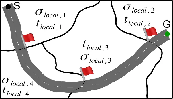
Figure 1. Operating environment with domains of different $${\sigma }_{\mathrm{l}\mathrm{o}\mathrm{c}\mathrm{a}\mathrm{l},j}$$ and $${t}_{\mathrm{l}\mathrm{o}\mathrm{c}\mathrm{a}\mathrm{l},j}$$ performance requirements for lateral vehicle motion control. Flags indicate points where requirements change as the vehicle transitions from one operating domain to another.
3.1.3. Responsiveness Quotient
The different hardware and software choices made when implementing a capability result in various response rates. This determines the responsiveness of a capability. Let $${f}_{\mathrm{m}\mathrm{i}\mathrm{n}}$$ be the minimum allowable response rate in hertz, and let $${f}_{\mathrm{a}\mathrm{c}\mathrm{t}}$$ be the actual response rate in hertz. Then, the condition
is sufficient for ensuring that the actual response rates are always bounded by the minimum allowable response rate.
When the inequality $${{f}_{\mathrm{a}\mathrm{c}\mathrm{t}}\ge f}_{\mathrm{m}\mathrm{i}\mathrm{n}}$$ is reformulated as in Equation (12), where frequency is converted into cycle time, it yields another benchmarking metric, $${C}_{\mathrm{r}\mathrm{e}\mathrm{s},i}$$, for a capability $$i$$ that is normalized and comparable across different system capabilities, scales or measurement units, called the responsiveness quotient.
Although this quotient is ill-formed when $${t}_{\mathrm{a}\mathrm{c}\mathrm{t},i}=0$$, in practice, $${t}_{\mathrm{a}\mathrm{c}\mathrm{t},i}>0$$, since the maximum computation rate is bounded by Bremermann’s limit, which is greater than zero. For practical purposes, the invalid region of Equation (12) is defined as zero, resulting in a piecewise function indicated in Equation (13) and visually presented in Figure 2.
The resulting responsiveness measure is dimensionless and, in the range, $$0\le {C}_{\mathrm{r}\mathrm{e}\mathrm{s},i}\le {k}^{-1}\cdot{t}_{\mathrm{m}\mathrm{a}\mathrm{x},i}\cdot \alpha$$, where $$k$$ is the number of operations per cycle and 𝛼 is the corrected Bremermann’s limit [19]. It should also be mentioned that the response rate is directly proportional to the complexity of the underlying algorithm and computing hardware performance, hence, it is assumed to be conserved.
Some changes in the environment depend on the response rate, but others are independent of it. Therefore, the minimum allowable response rate has to be selected in such a way that it is at least as great as the fastest rate of change in the operating domain.
A capability $$i$$ is autonomously feasible with respect to responsiveness if $${C}_{\mathrm{r}\mathrm{e}\mathrm{s},i}\ge 1$$. This is a necessary but insufficient condition for unconditional, fully autonomous functioning.
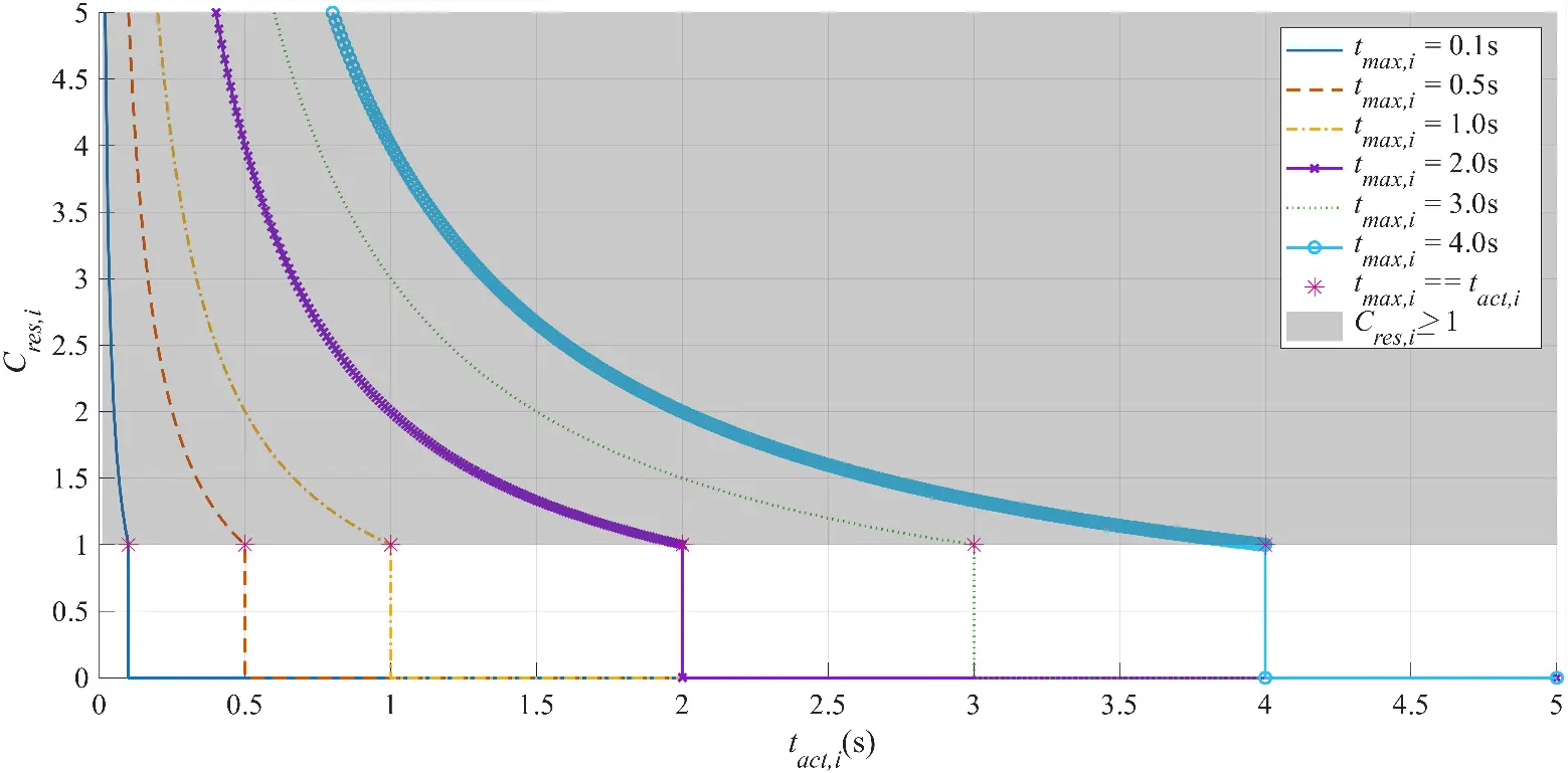
Figure 2. Plot of $${C}_{\mathrm{r}\mathrm{e}\mathrm{s},i}$$ for several $${t}_{\mathrm{m}\mathrm{a}\mathrm{x},i}$$ values.
As a demonstration, let us extend the autonomous driving task in the previous sub-section by imposing response rate requirements on each of the operating domains as indicated in Figure 1. Then, if
where $${t}_{\mathrm{g}\mathrm{l}\mathrm{o}\mathrm{b}\mathrm{a}\mathrm{l},i}=\mathrm{m}\mathrm{i}\mathrm{n}\left\{{t}_{\mathrm{l}\mathrm{o}\mathrm{c}\mathrm{a}\mathrm{l},1},\cdots ,{t}_{\mathrm{l}\mathrm{o}\mathrm{c}\mathrm{a}\mathrm{l},j},\cdots ,{t}_{\mathrm{l}\mathrm{o}\mathrm{c}\mathrm{a}\mathrm{l},m}\right\}$$, fulfilling this requirement indicates unconditional full autonomous functioning ability for that capability in all the $$m$$ operating domains. But if $${t}_{\mathrm{a}\mathrm{c}\mathrm{t},i}>{t}_{\mathrm{g}\mathrm{l}\mathrm{o}\mathrm{b}\mathrm{a}\mathrm{l},i}$$, then the associated full autonomous functioning ability is conditioned on responsiveness and is only locally functional in operating domains where $${t}_{\mathrm{a}\mathrm{c}\mathrm{t},i}\le {t}_{\mathrm{l}\mathrm{o}\mathrm{c}\mathrm{a}\mathrm{l},i}$$.
The proposed metrics are formulated in such a way as to monitor compliance with performance requirements, hence providing a means of regulating and ensuring safety. In the next section, two measures of autonomy, namely level and degree of autonomy, are discussed.
3.2. Level of Autonomy and Degree of Autonomy
Now that we have the metrics, we can use them to quantify autonomy. Given a set of requisite capabilities $$R$$ of cardinality $$n$$, a set of available capabilities of a system $$S$$, and a set of operating domains $$D$$ of cardinality $$m$$ and their associated performance requirements. Applying them to the process illustrated in Figure 3 yields the LoA (Level of Autonomy). Although neither reliability nor responsiveness is a sufficient condition for full autonomous functioning, their logical combination, i.e.,
is sufficient, and constitutes the primary test for LoA as indicated in Figure 3.
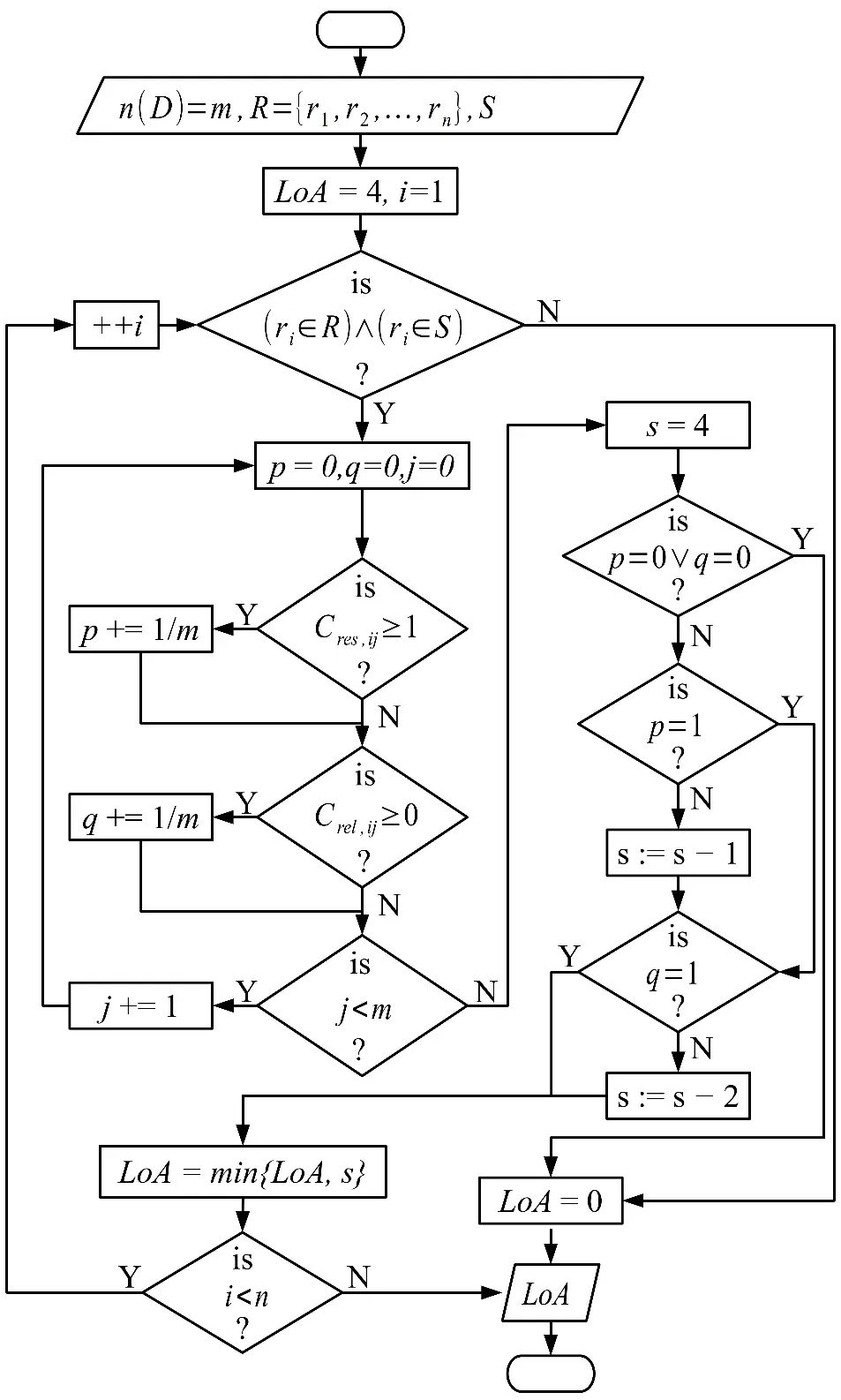
The output of the process in Figure 3 is an index associated with a description of the expected nominal performance of fully autonomous systems at that level. The levels are usually presented in a level chart. This work applied a five-level chart in Table 3, which was derived from the ten-level chart in Table 4 by grouping the ten levels into two categories, namely a category that does and a category that does not support control by an external operator. Since the focus is on full autonomous functioning, all levels in the former category were consolidated into level 0 of Table 3. In this cart, reliability-conditioned full autonomy is a level below responsive-conditioned full autonomy because reliability is associated with safety and consistent system performance.
Table 3. Levels of full autonomy in the relevant environment.
|
Level |
Description |
|---|---|
|
4 |
Unconditional full autonomy |
|
3 |
Responsiveness-conditioned full autonomy |
|
2 |
Reliability-conditioned full autonomy |
|
1 |
Responsiveness-conditioned and reliability-conditioned full autonomy |
|
0 |
Externally controlled or supervised autonomous functioning |
Table 4. Levels of autonomy in the relevant environment.
|
Level |
Description |
Operator Involvement |
|---|---|---|
|
9 |
Unconditional full autonomy |
No external operator |
|
8 |
Responsiveness-conditioned full autonomy |
|
|
7 |
Reliability-conditioned full autonomy |
|
|
6 |
Responsiveness-conditioned and reliability-conditioned full autonomy |
|
|
5 |
Full autonomous functioning with on-request supervision |
External operator |
|
4 |
Full autonomous functioning with continuous supervision |
|
|
3 |
System proposes course of action, operator approves or modifies it for the system to execute |
|
|
2 |
System proposes course of action for the operator to approve or modify and execute |
|
|
1 |
Operator determines and provides course of action for the system to execute |
|
|
0 |
Externally operated or remotely controlled |
LoA assesses the existence of requisite capabilities and whether their performances meet the requirements. However, it does not account for their actual performance, which is also of interest in indicating the performance quality of the capability. This is what DoA (Degree of Autonomy) achieves, and it is evaluated using the formulation in Equation (16) or Equation (17). The terms in these expressions model the universal trade-off between speed and precision. Under the zero-mean assumption (as in a random walk), variance is proportional to the expected power of error [20]. Hence, this DoA formulation is analogous to average kinetic energy in a system.
The DoA model in Equation (16) assumes capabilities to be of equal importance, but this need not always be the case. When essential capabilities are assigned different importance weights, the weighted model in Equation (17) should be applied instead.
To summarize, DoA always requires LoA to give it context. Otherwise, by itself, it is meaningless. Also, the fact that it can have a value of zero reinforces this.
4. Integrity of Autonomous Functioning
The first step towards ensuring that autonomous systems perform in accordance with requirement specifications is through product certification. As with all products, this certification should follow extensive system testing under all conceivable operating conditions over a specified period of time. This is not only a laborious and time-consuming undertaking, but also past performance cannot guarantee future performance for complex systems because real-world environments are complex and include a vast range of edge cases. Therefore, systems tested in controlled or limited conditions may not perform acceptably under rare or unforeseen scenarios such as extreme weather or agents exhibiting erratic behavior. Rare cases are often underrepresented in average-case performance, yet they can have a disproportionate impact on safety. This raises the need for online performance monitoring to ensure regularity in performance, and this is the purpose of integrity monitors.
Integrity is well studied in the aviation industry, specifically in relation to localization based on GNSS (Global Navigation Satellite System). It is parameterized by protection level (PL), alert limit (AL), time to alert (TTA), and integrity risk (IR) [21]. For fully autonomous systems that do not support external intervention, TTA is irrelevant. Therefore, we model integrity as a function of only PL, AL, and IR.
Failure of any requisite capability constitutes a safety risk, which should be properly managed. Herein, a safety risk is defined as the likelihood of a hazard and evaluated using Equation (18), where $$\rho$$ is the probability of failure and $$c\in \left[{c}_{\mathrm{m}\mathrm{i}\mathrm{n}},{c}_{\mathrm{m}\mathrm{a}\mathrm{x}}\right]$$ is the severity. Therefore, $$h$$ is a weighted severity. By asserting that failure of any requisite capability constitutes a hazard of the highest severity, then severity becomes a constant, $$c={c}_{\mathrm{m}\mathrm{a}\mathrm{x}}$$. Upon normalizing, Equation (18) simplifies to $$h=\rho$$, which gives the probability of a hazardous situation and will be referred to as the integrity risk.
To establish the probability of failure, we adopted the continuous mode ASIL D (Automotive Safety Integrity Level D) of ISO 26262-9 [22] for all essential capabilities, which on average is $${10}^{-7}$$ failures per operating hour. Assuming a constant failure rate and exponential distribution, this corresponds to a reliability of 99.99999% and a confidence interval of $$±5.326724\sigma$$. Substituting into Equation (9) gives
which is identical to Equation (9). To avoid ambiguity, the numerator and denominator must be represented to the same number of standard deviations. The reliability condition $${C}_{\mathrm{r}\mathrm{e}\mathrm{l},i}\ge 0$$ now implies that $$5.326724{\sigma }_{\mathrm{m}\mathrm{a}\mathrm{x},i}$$ is the 99.99999th percentile of the expected error, which in an integrity context corresponds to$$\,A{L}_{i}$$. The term $$5.326724{\sigma }_{\mathrm{a}\mathrm{c}\mathrm{t},i}$$ is the estimated statistical bounds on actual error that guarantees that the probability of the absolute error exceeding $$A{L}_{i}$$ is not greater than $$I{R}_{i}$$ and herein denoted as $$P{L}_{i}$$. The integrity monitor then tracks the reliability condition
at time instances $$k>0$$ for all essential capabilities and triggers an integrity loss event if violated.
The responsiveness quotient does not contribute to the integrity analysis because it is assumed to be conserved (see Section 3.1.3) and is therefore associated with zero risk. Furthermore, all capabilities are assumed to be continuously available throughout the entire operating time. Because the actual error is normally not directly measurable, PL is applied and can be estimated using state estimation algorithms. Unfortunately, linear and smug estimators may exhibit divergence and overconfidence, respectively, leading to unreliable error-bounds estimates and hence, safety problems. But with strategic redundancy and sensing modality diversification, the occurrence of such problems can be greatly minimized [23].
5. Demonstration Case Studies
In this section, application demonstrations of the proposed framework are presented. The demonstrations include an autonomous dynamic driving task application and an analysis of the DARPA (Defense Advanced Research Projects Agency) Subterranean (SubT) Challenge.
5.1. Autonomous Driving
On-road vehicles are a good example because of the great need to eliminate human drivers. Despite the necessity, this goal is being implemented gradually, with autonomous driving modules either cooperating with or collaborating with human drivers, or operating under human oversight. But the increase in uncertainty that comes with support for human intervention in the control process calls for development of more sophisticated control strategies. Additionally, having a human in the loop may lead to many variations in control architectures depending on the degree of human involvement, making it difficult to ensure reliability and assign liability in the event of mishaps. Also, with driver intervention, it is difficult to tell how the vehicle would ultimately perform. The solution to these challenges is full autonomous driving functionality.
To track full autonomous technology maturity as well as ensure its safe integration into vehicular traffic, several performance measures are applied. The most commonly used today include miles per disengagement, mean distance between interventions (MDBI), and mean time between interventions (MTBI) [24]. Unfortunately, measures based on a single metric are easily manipulated as per the Goodhart’s law. In contrast, our proposed framework is based on a diversified set of metrics, rendering it a good measure. Its application follows two sequential steps, namely LoA assessment and DoA evaluation.
The requisite capabilities for autonomous dynamic driving include longitudinal and lateral position control, heading control, longitudinal and lateral speed control, object detection, and local path planning. One can easily recognize these as the building blocks for driver-assistance technologies like lane keeping, adaptive cruise control, lane departure warning, and park assist. Then, as the goal is autonomous performance evaluation, all that is needed are performance requirements for each of the requisite capabilities. And like any other product, the only desiderata for allowance to participate in vehicular traffic would be conformance with those requirements.
This case study considers a simple world with two operating domains, namely motorways and built-up areas, and two arbitrary passenger service vans, namely vehicles A and B. Their performance requirements are listed in Table 5. The operating domain requirements are determined from the geometric characteristics of roadways, i.e., topology, curvature, width, and topography, and expert knowledge. The determination process adopted herein follows from control systems. In operation, a controlled system switches between open-loop and closed-loop phases, during and after computation, respectively. For increased safety and decreased uncertainty, the open-loop duration should be relatively small. Consider the recommended maximum longitudinal speed of 130 kmh−1 on German motorways and a longitudinal position $$AL$$ of 1.4 m from Table 5, the corresponding update rate is approximately 26 Hz. With the goal of keeping the uncertainty due to computation delay as low as possible, the update rate should be selected such that the resulting open-loop displacement is a fraction (we recommend at most 20%) of $$AL$$. For example, with $$5×26$$ Hz, the open-loop distance is 0.28 m, whereas with 150 Hz and 200 Hz it is 0.24 m and 0.18 m respectively. For generality and ease of evaluation, road segments with comparable geometric and topographic properties are governed by identical requirements. Although the protection levels of the vehicles are random variables, for the sake of demonstration we assumed them to converge to those given constant values. The response time of the vehicles’ capabilities is the period of their control/decision loops.
Table 5. Dynamic driving task requirements for a passenger vehicle and two arbitrary passenger vehicles’ specifications.
|
i |
Capability |
Motorways |
Built-Up Areas |
IR (FPH) c |
Vehicle A |
Vehicle B |
||||
|---|---|---|---|---|---|---|---|---|---|---|
|
$$\boldsymbol{AL_i}$$ |
$$\boldsymbol{f_{min,i}}$$ |
$$\boldsymbol{AL_i}$$ |
$$\boldsymbol{f_{min,i}}$$ |
$$\boldsymbol{PL_i}$$ |
$$\boldsymbol{f_{act,i}}$$ |
$$\boldsymbol{PL_i}$$ |
$$\boldsymbol{f_{act,i}}$$ |
|||
|
1 |
Longitudinal position control |
1.40 m a |
150 Hz |
0.29 m a |
150 Hz |
10−8 |
1.00 m |
200 Hz |
0.15 m |
160 Hz |
|
2 |
Lateral position control |
0.57 m a |
150 Hz |
0.29 m a |
150 Hz |
10−8 |
0.30 m |
200 Hz |
0.15 m |
160 Hz |
|
3 |
Heading control |
1.5° a |
150 Hz |
0.5° a |
150 Hz |
10−8 |
1.0° |
200 Hz |
0.3° |
160 Hz |
|
4 |
Longitudinal speed control |
4.1 kmh−1 b |
150 Hz |
3.0 kmh−1 b |
150 Hz |
10−8 |
2.0 kmh−1 |
200 Hz |
2.0 kmh−1 |
160 Hz |
|
5 |
Lateral speed control |
1.0 kmh−1 |
150 Hz |
1.4 kmh−1 |
150 Hz |
10−8 |
0.7 kmh−1 |
200 Hz |
1.0 kmh−1 |
160 Hz |
|
6 |
Object detection |
95% |
10 Hz |
95% |
10 Hz |
10−7 |
98% |
20 Hz |
96% |
15 Hz |
|
7 |
Local path planning |
95% |
10 Hz |
95% |
10 Hz |
10−6 |
99% |
20 Hz |
98% |
15 Hz |
a Values adopted from [25]. Based on lane width of 3.6 m and top speed of 137 kmh−1 on motorways, and lane width of 3 m and minimum road curvature of 20 m or width of 3.3 m and road curvature of 10 m for built-up areas. b Tolerance of vehicular traffic speed sensors on German roads is 3% for speeds over 100 kmh−1. c Faults per hour.
LoA assessment of the two vehicles with respect to each of the operating domains started by determining the variances and response times for each capability, and their corresponding metric scores, presented in Table 6 and Table 7, respectively. Then, applying the individual metric scores in Table 7 through the level of full autonomy check in Figure 3 yielded LoA 2 for vehicle A and LoA 4 for vehicle B. This meant that both vehicles possessed the requisite capabilities, but the autonomy of vehicle A is conditioned on reliability, as some of its protection levels are insufficient for built-up areas. Vehicle B possesses unconditional autonomy in this two-region world. To determine their actual performances, the DoA is evaluated, which is $$1560×{10}^{-3}$$ for vehicle A on the motorways, and $$842×{10}^{-3}$$ and $$762×{10}^{-3}$$ for vehicle B on the motorways and built-up areas, respectively. Although vehicle A outperforms vehicle B on the motorway, it cannot operate reliably in built-up areas. The $${10}^{-3}$$ term accounts for three decimal places, which we found to be sensitive to even the slightest change in any of the metrics. DoA is in the range $$0\le DoA\le +\infty$$ and higher values correspond to better performance.
Table 6. The corresponding variances and response times.
|
i |
Capability |
Motorways |
Built-Up Areas |
Vehicle A |
Vehicle B |
||||
|---|---|---|---|---|---|---|---|---|---|
|
$${\bm{\sigma }}_{\mathbf{m}\mathbf{a}\mathbf{x},\bm{i}}$$ a |
$$\boldsymbol{t_{\mathrm{\bf{max}},i}\,({s})}$$ |
$${\bm{\sigma }}_{\mathbf{m}\mathbf{a}\mathbf{x},\bm{i}}\mathrm{ }$$a |
$$\boldsymbol{t_{\mathrm{\bf{max}},i}\,({s})}$$ |
$${\bm{\sigma }}_{\mathbf{a}\mathbf{c}\mathbf{t},\bm{i}}\mathrm{ }$$a |
$$\boldsymbol{t_{\mathrm{\bf{act}},i}\,({s})}$$ |
$${\bm{\sigma }}_{\mathbf{a}\mathbf{c}\mathbf{t},\bm{i}}\mathrm{ }$$a |
$$\boldsymbol{t_{\mathrm{\bf{act}},i}\,({s})}$$ |
||
|
1 |
Longitudinal position control |
0.24430 |
0.00667 |
0.0506 |
0.00667 |
0.1745 |
0.0050 |
0.02617 |
0.00625 |
|
2 |
Lateral position control |
0.09946 |
0.00667 |
0.0506 |
0.00667 |
0.05235 |
0.0050 |
0.02617 |
0.00625 |
|
3 |
Heading control |
0.26175 |
0.00667 |
0.08725 |
0.00667 |
0.17450 |
0.0050 |
0.05235 |
0.00625 |
|
4 |
Longitudinal speed control |
0.71544 |
0.00667 |
0.52349 |
0.00667 |
0.34900 |
0.0050 |
0.34900 |
0.00625 |
|
5 |
Lateral speed control |
0.17450 |
0.00667 |
0.24430 |
0.00667 |
0.12215 |
0.0050 |
0.17450 |
0.00625 |
|
6 |
Object detection |
0.04092 b |
0.10 |
0.04092 b |
0.10 |
0.02628 b |
0.050 |
0.03679 b |
0.0667 |
|
7 |
Local path planning |
0.04455 b |
0.10 |
0.04455 b |
0.10 |
0.02034 b |
0.050 |
0.02862 b |
0.0667 |
a Each inherits the same units as in Table 5. b Assumed one independent trial, such that $$n=1$$.
Table 7. Reliability and responsiveness metrics values for vehicles A and B on the motorways and built-up areas. In bold are the capabilities for which the condition $${C}_{rel}\ge 0$$ is violated, therefore are non-functional.
|
i |
Capability |
Vehicle A |
Vehicle B |
||||||
|---|---|---|---|---|---|---|---|---|---|
|
Motorways |
Built-Up Areas |
Motorways |
Built-Up Areas |
||||||
|
$${\bm{C}}_{\bm{r}\bm{e}\bm{l},\bm{i}}$$ |
$${\bm{C}}_{\bm{r}\bm{e}\bm{s},\bm{i}}$$ |
$${\bm{C}}_{\bm{r}\bm{e}\bm{l},\bm{i}}$$ |
$${\bm{C}}_{\bm{r}\bm{e}\bm{s},\bm{i}}$$ |
$${\bm{C}}_{\bm{r}\bm{e}\bm{l},\bm{i}}$$ |
$${\bm{C}}_{\bm{r}\bm{e}\bm{s},\bm{i}}$$ |
$${\bm{C}}_{\bm{r}\bm{e}\bm{l},\bm{i}}$$ |
$${\bm{C}}_{\bm{r}\bm{e}\bm{s},\bm{i}}$$ |
||
|
1 |
Longitudinal position control |
0.48980 |
1.33333 |
−10.89060 |
1.33333 |
0.98852 |
1.06667 |
0.73246 |
1.06667 |
|
2 |
Lateral position control |
0.72299 |
1.33333 |
−0.07015 |
1.33333 |
0.93075 |
1.06667 |
0.73246 |
1.06667 |
|
3 |
Heading control |
0.55556 |
1.33333 |
−3.00000 |
1.33333 |
0.96000 |
1.06667 |
0.64000 |
1.06667 |
|
4 |
Longitudinal speed control |
0.76205 |
1.33333 |
0.55556 |
1.33333 |
0.76205 |
1.06667 |
0.55556 |
1.06667 |
|
5 |
Lateral speed control |
0.51000 |
1.33333 |
0.75000 |
1.33333 |
0.00000 |
1.06667 |
0.48980 |
1.06667 |
|
6 |
Object detection |
0.58737 |
2.00000 |
0.58737 |
2.00000 |
0.19158 |
1.50000 |
0.19158 |
1.50000 |
|
7 |
Local path planning |
0.79158 |
2.00000 |
0.79158 |
2.00000 |
0.58737 |
1.50000 |
0.58737 |
1.50000 |
5.2. DARPA Subterranean Challenge
This section analyses the DARPA SubT Challenge rules in light of the proposed metrics to show not only their prevalence, but also how their application can provide a self-evaluation measure indicative of a team’s likelihood of qualifying for such competitions prior to qualification rounds. The SubT robotics competition consisted of two categories, namely systems and virtual competitions. Both were aimed at motivating development of state-of-the-art solutions to navigation, mapping, and search tasks in dynamic, complex, and unknown subterranean environments [26]. In accomplishing those tasks, the competing systems utilized different sets of capabilities as indicated in Table 8.
Table 8. Requisite capability sets for DARPA SubT challenge tasks.
|
Capability |
Tasks |
Requirements |
|||
|---|---|---|---|---|---|
|
Navigation |
Mapping |
Searching |
$${\bm{A}\bm{L}}_{\bm{i}}$$ |
$${\bm{t}}_{\bm{m}\bm{a}\bm{x},\bm{i}}$$ |
|
|
Localization |
✔ |
✔ |
✔ |
5 m |
N.A. |
|
Motion planning |
✔ |
✔ |
✔ |
N.A. |
N.A. |
|
Motion control |
✔ |
✔ |
✔ |
N.A. |
N.A |
|
Mapping |
✔ |
✔ |
N.A. |
10 s a |
|
|
Communication |
✔ |
N.A. |
N.A. |
||
|
Path tracking |
✔ |
✔ |
N.A. |
N.A. |
|
|
Object detection |
✔ |
0.160 b |
N.A. |
||
|
0.099 c |
N.A. |
||||
a Communication delay is assumed insignificant compared to mapping time. b Uncertainty for virtual competition. c Uncertainty for systems competition. N.A. indicates the corrsponsing data were not available.
The scoring objective for the final trial runs in each category was the total number of accurately identified and localized artifacts within 60 min. To be valid, the position of the artifact had to be within ±5 m of the true position. Since the artifacts were spatially distributed within the environment and time was limited, this implicitly bounded the exploration speed. The systems competition was evaluated based on one final run, which did not account for variability in performance, whereas in the virtual competition, the final score was averaged on $$m$$ scenarios and $$n$$ trial runs per scenario to account for variability in performance.
Considering the aim of reporting all artifacts, and the fact that both competitions allowed five false reports yielded a combined uncertainty of correct identification and localization of an artifact of 0.099 and 0.160 for systems and virtual competitions, respectively. The other indirectly specified requirements are the map update rate, inferable from the 0.1 Hz frequency of the mapping and map transfer processes, and localization tolerance, inferable from the ±5 m artifact localization standard deviation. Nevertheless, as evident from the right-hand side of Table 8, most of the requirements were left for the developers to specify. Therefore, developers of successful competing systems had to conduct additional requirements elicitation to guide the design specification of their vehicles.
Although implicit and missing performance requirements offer development flexibility, as various capability-level performance combinations could meet the desired task-level performance. This flexibility comes at a cost of lost regulation at the capability level. Hence, it could jeopardizing the safety of the environment.
6. Conclusions
Autonomy quantification provides a means for matching full autonomous performance to task requirements, but has been complicated by a lack of clear terminology and consistent metrics. Our solution to these problems is the capability-based assessment framework presented herein. The framework is based on three quantitative metrics, namely essential capability set, reliability factor and responsiveness quotient. These were derived from relating human-job to robot-task characteristics. With the metrics as inputs, the framework outputs a dual-measure of autonomy featuring an interval-scale LoA and its associated ratio-scale DoA. LoA assesses the existence and compliance of essential capability performance with specified performance requirements, whereas DoA quantifies the actual performance of the system.
The framework has been demonstrated on an on-road dynamic driving task to show its ease of application. Furthermore, the prevalence and relevance of the underlying metrics have been demonstrated through analysis of the DARPA SubT Challenge competition rules. Besides being easily obtainable, the metrics fall on continuous ranges. Hence, satisfying the three desired characteristics of autonomy metrics, namely easily measurable, broad enough to capture autonomy evolution, and with good output resolution.
The physical interpretation of reliability and responsiveness metrics is robustness and execution frequency, respectively. This points to a parallelism with the universal trade-off of precision and speed. Hence, rendering them good indicators of performance. Furthermore, the mechanism of conditioning actual performance on required performance provides a regulatory interface for enforcing safety and design requirements, an idea inspired by the control and cybernetic loops. Additionally, this choice addresses the “what-ifs” surrounding autonomy, like what if one system has more sensors? What if one system has faster sensors? What if one system has a faster processor? To mention but a few. Therefore, it is our conviction that there is no need for an autonomy assessment framework to extend its analysis to lower-level hardware or software specifications, where many variations exist, and little regulation can be exercised.
The framework also incorporates an integrity monitor capable of online tracking of changes in capability performance. Therefore, with appropriate performance requirements, we envision a boost in user acceptance of autonomous systems as they develop reliable expectations of their performance. Lastly, the framework is also extendable to multi-agent applications, as only a clear definition of capability and its requirements is needed.
Although impactful, the framework makes a number of assumptions, including orthogonality and concurrent execution of capabilities, knowledge of operating domain requirements, error distribution is of zero-mean and finite variance, and continuous availability of autonomous functionality, which may be impractical for some applications.
Ethics Statement
Not applicable.
Informed Consent Statement
Not applicable.
Data Availability Statement
The original contributions presented in this study are included in the article. Further inquiries can be directed to the corresponding author.
Funding
This research received no external funding.
Declaration of Competing Interest
The author declares no conflicts of interest.
References
- Singh S. Critical Reasons for Crashes Investigated in the National Motor Vehicle Crash Causation Survey; National Highway Traffic Safety Administration (NHTSA), US Department of Transportation: Washington, DC, USA, 2015. [Google Scholar]
- Rankin W. Meda investigation process. Boeing Commer. Aero 2007, 2, 15–21. Available online: http://pages.suddenlink.net/reed/aero.pdf (accessed on 5 November 2022).
- Clough BT. Metrics, Schmetrics! How the Heck Do You Determine a Uav’s Autonomy Anyway; Air Force Research Laboratory: Wright-Patterson AFB, OH, USA, 2002. [Google Scholar]
- Jackson E, Williams O, Buchan K. Achieving robot autonomy. In Proceedings of the 3rd Conference on Military Robotic Applications, Medicine Hat, AB, Canada, 9–12 September 1991. [Google Scholar]
- Lampe A, Chatila R. Performance measure for the evaluation of mobile robot autonomy. In Proceedings of the 2006 IEEE International Conference on Robotics and Automation, Orlando, FL, USA, 15–19 May 2006; pp. 4057–4062. DOI:10.1109/ROBOT.2006.1642325 [Google Scholar]
- Insaurralde CC, Lane DM. Autonomy-assessment criteria for underwater vehicles. In Proceedings of the 2012 IEEE/OES Autonomous Underwater Vehicles (AUV), Southampton, UK, 24–27 September 2012; pp. 1–8. DOI:10.1109/AUV.2012.6380746 [Google Scholar]
- Kendoul F. Towards a unified framework for uas autonomy and technology readiness assessment (atra). In Autonomous Control Systems and Vehicles; Springer: Tokyo, Japan, 2013; pp. 55–71. DOI:10.1007/978-4-431-54276-6_4 [Google Scholar]
- Clothier R, Williams B, Perez T. A review of the concept of autonomy in the context of the safety regulation of civil unmanned aircraft systems. In Proceedings of the Australian System Safety Conference 2013 (ASSC 2013) [Conferences in Research and Practice in Information Technology (CRPIT), Conferences in Research and Practice in Information Technology]; Australian Computer Society Inc.: Sydney, Australia, 2014; pp. 15–27. [Google Scholar]
- Elbanhawi M, Mohamed A, Clothier R, Palmer JL, Simic M, Watkins S. Enabling technologies for autonomous mav operations. Prog. Aerosp. Sci. 2017, 91, 27–52. DOI:10.1016/j.paerosci.2017.03.002 [Google Scholar]
- Huang H-M, Messina E, Albus J. Autonomy Levels for Unmanned Systems (Alfus) Framework, Volume II: Framework Models Version 1.0. 2007. Available online: https://nvlpubs.nist.gov/nistpubs/Legacy/SP/nistspecialpublication1011-II-1.0.pdf (accessed on 13 April 2022). DOI:10.6028/NIST.SP.1011-II-1.0
- On-Road Automated Driving (ORAD) Committee. Taxonomy and Definitions for Terms Related to Driving Automation Systems for On-Road Motor Vehicles; SAE International: Warrendale, PA, USA, 2021. DOI:10.4271/J3016_202104 [Google Scholar]
- California Department of Motor Vehicles. California Code of Regulations Title 13, Division 1, Chapter 1, Article 3.7—Testing of Autonomous Vehicles. 2025. Available online: https://www.dmv.ca.gov/portal/uploads/2020/06/Adopted-Regulatory-Text-2019.pdf (accessed on 17 September 2022).
- Chrystal KA, Mizen PD, Mizen P. Goodhart’s law: Its origins, meaning and implications for monetary policy. Cent. Bank. Monet. Theory Pract. Essays Honour Charles Goodhart 2003, 1, 221–243. DOI:10.4337/9781781950777 [Google Scholar]
- Doboli A, Curiac D, Pescaru D, Doboli S, Tang W, Volosencu C, et al. Cities of the future: Employing wireless sensor networks for efficient decision making in complex environments. arXiv 2018, arXiv:1808.01169. DOI:10.48550/arXiv.1808.01169 [Google Scholar]
- Curtin TB, Crimmins DM, Curcio J, Benjamin M, Roper C. Autonomous underwater vehicles: Trends and transformations. Mar. Technol. Soc. J. 2005, 39, 65–75. DOI:10.4031/002533205787442521 [Google Scholar]
- Russell SJ. Artificial Intelligence a Modern Approach; Pearson Education, Inc.: Hoboken, NJ, USA, 2010. [Google Scholar]
- Hasslacher B, Tilden MW. Living machines. Robot. Auton. Syst. 1995, 15, 143–169. DOI:10.1016/0921-8890(95)00019-C [Google Scholar]
- Lytle CW. Job Evaluation Methods; Ronald Press: Santa Fe, NM, USA, 1946; pp. 56–58. [Google Scholar]
- Gorelik G. Bremermann’s limit in cgh-physics. arXiv 2009, arXiv:0910.3424. DOI:10.48550/arXiv.0910.3424 [Google Scholar]
- Ogata K. Discrete-Time Control Systems; Prentice-Hall, Inc.: Upper Saddle River, NJ, USA, 1995; p. 9. [Google Scholar]
- ICAO. International standards and recommended practices. In Annex 10 to the Convention on International Civil Aviation; International Civil Aviation Organization: Montreal, QC, Canada, 2018; Volume 1. [Google Scholar]
- International Organization for Standardization. ISO 26262-9:2018 Road Vehicles—Functional Safety—Part 9: Automotive Safety Integrity Level (ASIL)-Oriented and Safety-Oriented Analyses; International Organization for Standardization: Geneva, Switzerland, 2018. [Google Scholar]
- Wang X, Chen T, Wang R, Lu J, Dou G. Review of state estimation methods for autonomous ground vehicles: Perspectives on estimation objects, vehicle characteristics, and key algorithms. Sensors 2025, 25, 3927. DOI:10.3390/s25133927 [Google Scholar]
- Paz D, Lai PJ, Chan N, Jiang Y, Christensen HI. Autonomous vehicle benchmarking using unbiased metrics. In Proceedings of the 2020 IEEE/RSJ International Conference on Intelligent Robots and Systems (IROS), Las Vegas, NV, USA, 24 October 2020–24 January 2021; pp. 6223–6228. DOI:10.1109/IROS45743.2020.9340902 [Google Scholar]
- Reid TG, Houts SE, Cammarata R, Mills G, Agarwal S, Vora A, et al. Localization requirements for autonomous vehicles. SAE Int. J. Connect. Autom. Veh. 2019, 2, 173–190. DOI:10.4271/12-02-03-0012 [Google Scholar]
- Darpa Subterranean Challenge: Competition Rules Final Event. Available online: https://github.com/subtchallenge/official_docs/blob/main/SubT_Challenge_Finals_Rules.pdf (accessed on 1 October 2023).