Critical Conservation Gaps for Microendemic Axolotls Reveal Inadequate Protection in Central Mexico

Critical Conservation Gaps for Microendemic Axolotls Reveal Inadequate Protection in Central Mexico
Briggite I. Araiza-Alvarado 1 Alberto González-Zamora 2 Héctor A. Castro-Bastidas 3 Julián A. Velasco 4 David R. Aguillón-Gutiérrez 1,*
Received: 28 February 2026 Revised: 30 March 2026 Accepted: 28 April 2026 Published: 12 May 2026

© 2026 The authors. This is an open access article under the Creative Commons Attribution 4.0 International License (https://creativecommons.org/licenses/by/4.0/).
1. Introduction
Global amphibian populations face unprecedented declines driven by habitat loss, climate change, invasive species, and emerging diseases such as chytridiomycosis [1,2]. Mexico, a biodiversity hotspot with more than 400 amphibian species [3], exhibits remarkable microendemic diversity, particularly in the Trans-Mexican Volcanic Belt (TMVB), a region shaped by volcanic activity and pronounced elevational gradients [4,5]. In this area, 92.3% of salamanders of the genus Ambystoma are classified as threatened according to the International Union for Conservation of Nature (IUCN) Red List, and 100% are protected under Mexico’s NOM-059-SEMARNAT [6].
Four Ambystoma species from the TMVB are categorized as Critically Endangered (CR): A. amblycephalum, A. andersoni, A. dumerilii, and A. mexicanum. These microendemics are confined to isolated aquatic systems in central Mexico. Ambystoma amblycephalum inhabits high-elevation streams in Michoacán, with recent rediscoveries suggesting fragmented remnant populations [7]. Ambystoma andersoni and A. dumerilii are lacustrine endemics restricted to Lakes Zacapu and Pátzcuaro, respectively [8,9], while the iconic A. mexicanum persists only in the southern remnants of Lake Xochimilco [10].
Their restricted distributions, dependence on permanent water bodies, and sensitivity to disturbances render these species highly vulnerable. Habitat fragmentation caused by urbanization, intensive agriculture, pollution, and invasive species (such as predatory fish and the African clawed frog Xenopus laevis) has severely reduced population connectivity [10,11,12]. Critical areas such as Bosque de Agua and Xochimilco exhibit major protection gaps, with only limited coverage of suitable habitat within protected areas [10,11]. This highlights the urgent need to accurately assess areas of occupancy and ecosystem integrity to guide targeted conservation actions.
Despite their high ecological and cultural importance, conservation efforts in central Mexico remain inadequate. Existing protected areas (PA) often fail to encompass key breeding sites or dispersal corridors, increasing functional isolation and extinction risk [13]. Emerging threats, such as chytridiomycosis, have intensified declines in related Ambystoma species, demanding immediate action [14]. Understanding the extent of protection and ecosystem integrity for these four species is essential to prioritizing conservation strategies in the TMVB, where amphibians can serve as indicators of overall ecosystem health.
Our analysis reveals critical protection gaps, emphasizing the need for expansion of protected areas, connectivity restoration, and targeted interventions to mitigate ongoing declines and strengthen resilience against climatic and anthropogenic pressures.
2. Materials and Methods
2.1. Data Source
A total of 148 presence records for the four species were initially obtained from Global Biodiversity Information Facility (GBIF) and specialized literature. Following rigorous depuration to remove duplicates, records with metadata errors (e.g., imprecise coordinates or outside known geographic range), and cross-verification with Amphibian Species of the World [15], 89 valid records were retained: nine for A. amblycephalum, eight for A. andersoni, 36 for A. dumerilii and 36 for A. mexicanum. These depurated records served as the basis for all subsequent spatial and environmental analyses.
2.2. Determination of Distribution Areas
Initially, we calculated the extent of occurrence (EOO) using minimum convex polygons (MCP) in QGIS 3.40.15 (Bratislava) from the depurated records (compiled, cleaned, and validated), following IUCN recommendations for delineating the general accessible area [16]. These polygons provide a clear and straightforward of each species’ approximate initial geographic distribution (Figure 1). However, since MCP tends to overestimate the actual distribution of species [17], and considering the strict microendemism of our study species with a strictly aquatic habitat and elevational dependence [18], we refined the areas using binary masks of optimal elevation extracted from the Mexican Elevation Continuum 4.0 (CEM 4.0) at 15 m resolution [19]. These masks were combined with specific hydrographic filters (hydrographic network) [20]: streams for A. amblycephalum and lakes for the remaining species, based on information from AmphibiaWeb, Amphibian Species of the World [15], and specialized literature. This procedure allowed us to obtain a more precise estimate of the occupied distribution (hereafter, refined areas of occupancy), thereby avoiding the overestimation inherent to MCP. Although we refer to our estimates as “refined areas of occupancy”, these do not correspond to the formal Area of Occupancy (AOO) of the IUCN (which is calculated using 2 × 2 km grid cells), but rather to a refinement of the MCP with environmental filters.
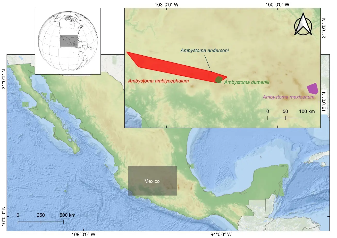
Figure 1. Minimum convex polygons (MCP) delineating the initial extent of occurrence (EOO) based on depurated records of the four Ambystoma species from central Mexico.
Additionally, we applied buffer zones to account for the limited mobility of these species: 100 m for A. amblycephalum [21], a stream species with occasional metamorphosis that enables limited terrestrial dispersal; and 50 m for the strictly paedomorphic lacustrine species A. andersoni, A. dumerilii and A. mexicanum [22], which remain permanently aquatic and exhibit minimal movement within their lake habitats. These buffers enabled the inclusion of transition zones and potential adjacent habitats.
2.3. Integration of Environmental Variables
From the depurated records, we extracted corresponding elevations using CEM 4.0 and calculated species-specific ranges through descriptive statistics (minimum and maximum elevation, median, and standard deviation), which helped delimit the refined areas of occupancy as described in the previous procedure. We incorporated land use and vegetation coverages from CONABIO [20] Series VII (30 m resolution), extracting the specific category for each record through spatial overlay in QGIS.
Climatic variables were derived from annual precipitation, maximum annual temperature, and minimum annual temperature data from MexHiResClimDB [23], a high-resolution (~500 m) database tailored to Mexico, ideal for species with restricted ranges. Monthly rasters of maximum temperature (tmax), minimum temperature (tmin), mean temperature (tmean), and precipitation (prec) for the period 1991–2020 were processed in R 4.3.1 [24] to generate the 19 standard bioclimatic variables (BIO1–BIO19; see Appendix A for complete variable definitions) by calculating monthly averages and applying moving-window functions for extreme quarters, following the procedure of Velasco and González-Salazar [25].
Bioclimatic values were extracted at presence points and analyzed through descriptive and exploratory statistical approaches in R (see Supplementary Material), including climatic space plots (BIO1 vs. BIO12) with 68% confidence ellipses, boxplots of key variables, principal component analysis (PCA), and bivariate density. For climatic space, we selected BIO1 (annual mean temperature) and BIO12 (annual precipitation) as the most relevant variables for delimiting thermal and hydrological niches in aquatic species dependent on permanent habitats [26,27]. Given their interpretative clarity and relevance for characterizing realized niches in this descriptive context, we prioritized the two-dimensional analysis with 68% ellipses (~1 SD), which focuses on the core of the realized niche and avoids the influence of outliers that would overestimate the potential niche [28]. Supplementary material includes a comparison with 95% ellipses (~2 SD) to explore peripheral variability.
2.4. Evaluation of Conservation Gaps and Effective Protection
To quantify the level of protection and vulnerability of the refined areas of occupancy for the four study species, we calculated two complementary indicators. As a positive conservation proxy, we determined the percentage of the distribution area overlapping with PA. Total areas of the refined polygons were calculated in km2, and intersection with the official PA layer [20] was performed to obtain the overlap percentage. This indicator reflects the extent of legal protection and potential management measures in the species’ distribution areas.
As a negative proxy, we used the Ecosystem Integrity Index (EII), a multifactorial indicator that assesses ecosystem health and functionality through the integration of metrics such as habitat fragmentation, biological connectivity, vegetation cover loss, and anthropogenic influence (e.g., roads, urbanization), based on satellite remote sensing data and spatial modeling [20,29]. The EII is normalized between 0 and 1 (base layer 2018 at 250 m), where values close to 0 indicate high degradation and low ecosystem integrity, and values close to 1 reflect ecosystems with high integrity and minimal alteration. This index provides a quantitative measure of environmental degradation across the distribution ranges, enabling identification of vulnerable areas beyond the mere presence of PA and highlighting cumulative impacts that could compromise the long-term viability of these threatened microendemic aquatic species. EII values were extracted directly from the national CONABIO [20] layer overlaid with the refined distribution polygons in QGIS, focusing on species-specific means and ranges to evaluate overall integrity.
3. Results
3.1. Spatial Distributions and Effective Protection
The refined areas of occupancy were small and varied widely in their level of effective protection (Table 1). Ambystoma amblycephalum exhibited the largest area (108.19 km2), followed by A. dumerilii (74.32 km2), A. mexicanum (15.14 km2), and A. andersoni with the most reduced (0.38 km2). Overlap with PA varied considerably: high in A. mexicanum (98.41%) and A. andersoni (86.84%), but null in A. dumerilii (0.00%) and very low in A. amblycephalum (4.79%). Mean EII values were generally low (0.05–0.43), with ranges indicating significant degradation in most occupied areas, particularly in A. dumerilii (mean 0.06 ± 0.07).
Table 1. Refined area of occupancy, overlap with Protected Areas (PA), and Ecosystem Integrity Index (EII, scale 0 = high degradation to 1 = high integrity) for four microendemic Ambystoma species in central Mexico.
|
Species |
Refined Area of Occupancy (km2) |
Protection in PA (km2/%) |
EII (Mean ± SD; Range) |
|---|---|---|---|
|
Ambystoma amblycephalum |
108.19 |
5.19/4.79% |
0.43 ± 0.23 (0.00–0.96) |
|
Ambystoma andersoni |
0.38 |
0.33/86.84% |
0.39 ± 0.23 (0.00–0.97) |
|
Ambystoma dumerilii |
74.32 |
0.00/0.00% |
0.06 ± 0.07 (0.00–0.26) |
|
Ambystoma mexicanum |
15.14 |
14.90/98.41% |
0.05 ± 0.12 (0.00–0.97) |
3.2. Altitudinal Characteristics and Land Use
Altitudinal ranges extracted from CEM 4.0 were remarkably narrow for all four species, reflecting their condition as strict microendemics dependent on specific aquatic habitats. Ambystoma amblycephalum presented the broadest range (1930–2014 m a.s.l.), while A. andersoni showed the most restricted (1984–1993 m a.s.l.). A. dumerilii had an intermediate range (2036–2359 m a.s.l.), and A. mexicanum recorded 2231–2343 m a.s.l. Central values (median) and variability (standard deviation), along with predominant land use and vegetation categories, are presented in Table 2.
This altitudinal narrowness is combined with a strong association to habitats altered by human activity: all species showed predominance of categories such as human settlements and rain-fed annual agriculture. Ambystoma amblycephalum was primarily linked to human settlements and rain-fed annual agriculture; A. andersoni to a mixture including tule and secondary vegetation; A. dumerilii exhibited the greatest diversity of uses (including irrigated agriculture, pine-oak forests, and induced grassland); and A. mexicanum to cultivated forest, halophytic grassland, and irrigated agriculture.
Table 2. Altitudinal ranges and main land use and vegetation categories (Series VII) associated with depurated presence records of four microendemic Ambystoma species in central Mexico.
|
Species |
Altitudinal Range (m) |
Median ± SD (m) |
Land Use and Vegetation Categories (Series VII) |
|---|---|---|---|
|
Ambystoma amblycephalum |
1930–2014 |
1972 ± 105.5 |
Human settlements, Rain-fed annual agriculture |
|
Ambystoma andersoni |
1984–1993 |
1987 ± 2.77 |
Human settlements, Tule, Rain-fed annual agriculture, Shrub secondary vegetation, Pine-oak forest, Oak forest, Induced grassland |
|
Ambystoma dumerilii |
2036–2359 |
2137 ± 85.5 |
Human settlements, Rain-fed and irrigated annual agriculture, Tule, Shrub/tree secondary vegetation of low deciduous forest, Pine-oak and oak forests, Induced grassland, Irrigated annual agriculture |
|
Ambystoma mexicanum |
2231–2343 |
2260 ± 28.69 |
Cultivated forest, Halophytic grassland, Rain-fed annual agriculture, Human settlements, Irrigated annual agriculture |
3.3. Climatic Niches
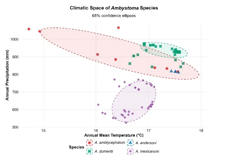
Values of annual mean temperature (BIO1) and annual precipitation (BIO12) revealed differentiated and notably restricted climatic niches among the four species (Table 3). Ambystoma andersoni presented the warmest and driest niche (BIO1: 17.5 °C, BIO12: 815 mm), with an extremely compact range. A. mexicanum showed the coldest conditions and lowest precipitation (BIO1: 16.7 °C, BIO12: 649 mm), while A. amblycephalum and A. dumerilii occupied intermediate positions, with greater precipitation variability. These patterns are represented in the two-dimensional climatic space (BIO1 vs. BIO12) with 68% confidence ellipses, where minimal overlap between species is observed, and a particularly compact cluster is evident in A. andersoni (Figure 2a).
Table 3. Mean values and ranges of annual mean temperature (BIO1, °C) and annual precipitation (BIO12, mm) extracted from MexHiResClimDB at the depurated presence records of the four Ambystoma species from central Mexico.
|
Species |
BIO1: Annual Mean Temperature (°C) |
BIO1 Range (°C) |
BIO12: Annual Precipitation (mm) |
BIO12 Range (mm) |
|---|---|---|---|---|
|
Ambystoma amblycephalum |
16.4 |
14.7–17.6 |
937 |
816–1066 |
|
Ambystoma andersoni |
17.5 |
17.4–17.6 |
815 |
811–818 |
|
Ambystoma dumerilii |
17.3 |
16.7–17.7 |
931 |
843–975 |
|
Ambystoma mexicanum |
16.7 |
16.0–17.1 |
649 |
526–771 |
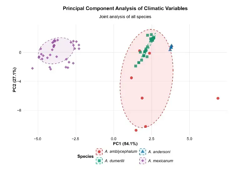
The joint principal component analysis (PCA) of the 19 bioclimatic variables confirmed a clear separation among species in multivariate space (Figure 2b). The first principal component (PC1, 54.1% explained variance) was primarily driven by temperature gradients (including BIO1, BIO5, BIO10, and BIO4), differentiating colder and more climatically seasonal niches (A. amblycephalum and A. mexicanum, negative and dispersed positions) from warmer and more stable ones (A. dumerilii and A. andersoni, positive and concentrated positions). The second component (PC2, 27.1% variance) was dominated by precipitation and seasonality-driven variables (mainly BIO12, BIO16, and BIO15), highlighting greater precipitation variability (both in total amount and seasonal distribution) for A. amblycephalum and A. mexicanum.
 |
 |
|
(a) |
(b) |
Figure 2. Climatic analysis of the four Ambystoma species in central Mexico: (a) Two-dimensional climatic space based on annual mean temperature (BIO1, °C) and annual precipitation (BIO12, mm); (b) Joint principal component analysis (PCA) of the 19 bioclimatic variables. Scores of the records are shown on PC1 (54.1% explained variance) vs. PC2 (27.1% explained variance). PC1 is dominated by temperature gradients (primarily BIO1, BIO5, BIO10, and BIO4); PC2 by precipitation and seasonality variables (primarily BIO12, BIO16, and BIO15). See Appendix A for the names of the bioclimatic variables. Note 1: sample sizes vary among species (n = 6–36), therefore, confidence ellipses represent central tendency rather than robust niche boundaries. Note 2: The 68% confidence ellipse for A. andersoni is present but not visible at this scale due to extreme niche compactness (area = 0.14 units2); see Table S1 for complete ellipse parameters.
Boxplots of key variables (BIO1, BIO12, BIO4, and BIO15) are presented in the Supplementary Material (Figure S1), highlighting greater thermal seasonality in A. dumerilii and A. mexicanum, and high precipitation seasonality (>95%) across all species, with greater dispersion in A. amblycephalum and A. dumerilii.
An exploratory comparison with 95% confidence ellipses is included in the Supplementary Material (Figure S2), which expands the climatic niche areas by an average factor of 2.63 relative to 68% (Table S1). This reveals marginal additional overlap in some species pairs, although central separation remains clear and the compactness of A. andersoni remains evident.
4. Discussion
4.1. Reduced Areas of Occupancy and Fragmentation as Defining Traits
The refined area of occupancy values obtained in this study differ notably from the official estimates reported by the IUCN for these species. While the IUCN reports an AOO of 18 km2 for A. amblycephalum [30], our results reveal a refined area of 108.19 km2, nearly six times larger. This discrepancy can be attributed primarily to the recent discovery of fragmented remnant populations in streams of the Michoacán region [7], which were not considered in the original 2016 assessment. Similarly, for A. andersoni we contrast our refined area of 0.38 km2 against an EOO of 0.35 km2 reported by the IUCN [31], showing consistency in the extreme restriction of its geographic range. For A. dumerilii, our area of 74.32 km2 exceeds the IUCN AOO of 6 km2 [32], likely due to the application of a 50 m buffer around Lake Pátzcuaro, which captures adjacent lacustrine habitats not included in the original assessment. Finally, A. mexicanum presents a refined area of 15.14 km2, considerably smaller than the EOO of 467 km2 reported by the IUCN [33], reflecting the drastic contraction of its distribution towards the southern remnants of Lake Xochimilco [10]. These comparisons underscore the importance of periodically updating threat assessments with recent field data and refined methodologies that incorporate specific environmental masks and filters for sensitive species such as these amphibians.
Our results reveal that the refined areas of occupancy for the four Ambystoma species are extremely small and markedly fragmented, with values ranging from 0.38 km2 in A. andersoni to 108.19 km2 in A. amblycephalum (Table 1). These extents are consistent with the strict microendemism pattern that characterizes salamanders in the TMVB [4,5], but highlight exceptional vulnerability when compared to other Neotropical amphibians. For example, the refined area of occupancy of A. andersoni (0.38 km2) represents less than 5% of the area reported for Pristimantis thymalopsoides in the Ecuadorian Andes (~8 km2) [34], a species already considered CR due to its extremely restricted distribution. It is even significantly smaller than that of miniaturized plethodontid salamanders of the genus Thorius in Mexico, such as T. tlaxiacus (~16 km2) [35], or that of Pseudoeurycea robertsi (8 km2) [36], another microendemic salamander from Nevado de Toluca categorized as CR. Even within Ambystoma, the range of A. andersoni is drastically smaller than that of A. tigrinum in North America (3,349,328 km2) [37] or A. gracile in the northwestern United States (807,275 km2) [38]. The reduced area of occupancy of A. andersoni, in particular, represents one of the most restricted geographic ranges documented for the genus, comparable only to isolated populations of Ambystoma in central Mexico [6].
4.2. Protection Gaps and Insufficient Nominal Protection
Unequal overlap with PA constitutes one of the most alarming findings. Although A. mexicanum and A. andersoni exhibit apparently high coverages (98.41% and 86.84%, respectively), these figures mask limited effective protection: the total area of A. andersoni is so small that even a high proportion represents less than 0.4 km2 under legal protection. More critically, A. amblycephalum and A. dumerilii show overlaps below 5%, placing them in a condition of “nominal protection” (presence in risk lists) where most of their distribution remains outside any conservation management scheme. This pattern of protection gaps aligns with recent diagnoses for A. altamirani in Bosque de Agua, where less than 2% of suitable habitat lies within a PA [11], pointing to a systemic crisis of coverage for aquatic microendemics in the region.
4.3. Ecosystem Degradation and Conservation Paradox
Ecosystem Integrity Index values between 0.05 and 0.43 confirm that even within the identified occupied areas, ecosystems have suffered severe degradation. The average of 0.06 ± 0.07 for A. dumerilii is particularly concerning, indicating that virtually its entire distribution in Lake Pátzcuaro operates under conditions of high anthropogenic disturbance. These levels are comparable to those reported for A. ordinarium in degraded pine-oak forests of Michoacán [39], and demonstrate that legal protection alone does not guarantee ecosystem functionality. The discrepancy between nominal protection (presence in risk lists) and actual habitat integrity represents a critical conservation paradox: the species are “protected on paper” but persist within functionally collapsed ecosystems [40], as quantified by the low EII values reported here.
4.4. Realized Climatic and Vulnerability to Global Change
The climatic conditions we identified (annual mean temperatures between 16–17.5 °C and precipitation of 650–930 mm) reflect climatic conditions associated with their restricted distributions that, while enabling the adaptive radiation of Ambystoma in the TMVB [4], currently constitute a factor of hypersensitivity. The narrow range of temperatures observed for A. andersoni (range 17.43–17.57 °C) and the low precipitation associated with A. mexicanum (526–771 mm) suggest limited tolerance margins in the face of increasing climatic variability. This specialization correlates with narrow altitudinal ranges (1930–2359 m a.s.l.), where modest upward shifts in distribution as projected for Mexican amphibians under climate change scenarios could result in the loss of thermally suitable habitats without upward migration alternatives due to the volcanic dome topography [5,12].
4.5. Persistence in Anthropized Matrices and “Refuge in Disturbance”
The dominance of anthropized land uses in presence records (human settlements, rain-fed and irrigated agriculture, secondary vegetation) indicates that remnant populations persist predominantly in highly anthropized landscapes. For A. amblycephalum, the association with rain-fed annual agriculture in high-mountain streams suggests forced dependence on modified hydrological systems, where hydrological regulation and agrochemical contamination represent constant threats. In A. mexicanum, the presence in cultivated forests and halophytic grasslands in southern Xochimilco documents historical contraction from natural lacustrine habitats to anthropogenic remnants [10], a “refuge in disturbance” pattern that, while enabling temporary persistence of the species, exposes populations to extreme fluctuations in water quality and competition with invasive species, and emerging diseases such as chytridiomycosis [10,14,41].
4.6. Syndrome of Risk Factors in TMVB Microendemics
Overall, these findings confirm that microendemism in Ambystoma of the TMVB constitutes a syndrome of risk factors: spatially restricted distributions, obligate dependence on permanent aquatic habitats, narrow realized climatic specialization, and location in landscapes dominated by human activity. Habitat fragmentation acts synergistically with these factors, reducing population connectivity at scales that compromise long-term demographic viability. The 50–100 m buffers zones applied, based on the limited mobility of these salamanders [21,22], likely underestimate real connectivity requirements for maintaining effective gene flow, particularly in A. amblycephalum, where metamorphosis in some individuals may temporarily increase terrestrial habitat needs. The convergence of these factors positions these four species on a trajectory of decline that, without urgent active management interventions, is at risk of extinction over the coming decades, replicating the pattern already observed in the extirpation of A. mexicanum from Lake Chalco and the severe contraction in Xochimilco [10,15].
4.7. Conservation Implications
Conservation strategies for aquatic microendemics in the TMVB must move beyond nominal protection toward active and integrated management. Based on our results and existing frameworks for threatened amphibians in Mexico [40], we recommend: (1) quantitative risk recategorization under revised IUCN criteria, accounting for actual occupancy areas and low ecosystem integrity values; (2) immediate creation of micro-reserves for species with ranges <1 km2, such as A. andersoni; (3) connectivity expansion through restored aquatic corridors; (4) systematic population monitoring with emphasis on emerging threats such as chytridiomycosis [14]; and (5) community involvement through sustainable management of individual private landholdings, ejidos (communal lands), and environmental education. The convergence of microendemism, climatic conditions associated with their restricted distributions, and anthropized matrices places these species on a trajectory of decline that can only be reversed through the simultaneous and urgent implementation of these measures.
Additionally, given the virtually impossible natural dispersal among these geographically isolated populations, assisted migration and controlled individual exchange programs should be evaluated as complementary conservation tools, provided that prior genetic characterization and strict biosecurity protocols are in place to minimize risks of disease transmission and disruption of locally adapted genotypes [14].
5. Conclusions
The gap between legal protection and effective protection for four microendemic Ambystoma species in the TMVB refined areas of occupancy ranging from 0.38 to 108.19 km2, null or minimal overlaps with protected areas in A. amblycephalum and A. dumerilii, and EII values revealing severe degradation across their entire distributions underscores the inadequacy of current conservation strategies for specialized aquatic amphibians in anthropized landscapes. Notably, our refined estimates for A. amblycephalum and A. dumerilii exceed previous IUCN assessments, reflecting the discovery of additional remnant populations and improved mapping resolution; however, these populations persist predominantly outside protected areas in functionally degraded ecosystems, meaning that the expanded distribution knowledge documented here does not translate into improved conservation or population viability. The combination of narrow climatic niches, restricted altitudinal ranges, and persistence in matrices dominated by agriculture and urbanization places these species on a trajectory of accelerated decline. This pattern can only be reversed through the immediate expansion of effective protected areas, restoration of connectivity between fragmented habitats, and integrated adaptive management with local communities. Our results demonstrate that microendemism in the TMVB is not merely a biogeographic attribute but a synergistic risk factor that urgently demands prioritizing this region as a critical hotspot for global amphibian conservation.
Supplementary Materials
The following supporting information can be found at: https://www.sciepublish.com/article/pii/1002, Figure S1: Boxplots of key bioclimatic variables for the four Ambystoma species: BIO1 (annual mean temperature, °C), BIO12 (annual precipitation, mm), BIO4 (temperature seasonality), and BIO15 (precipitation seasonality). The boxplots show the median (central line), interquartile range (box), and full range (whiskers); Figure S2: Exploratory comparison of climatic niches with 95% confidence ellipses. (a) Two-dimensional climatic space based on annual mean temperature (BIO1, °C) vs. annual precipitation (BIO12, mm), with points by species and 95% ellipses; (b) Joint principal component analysis (PCA) of the 19 bioclimatic variables with 95% ellipses; Table S1: Comparison of confidence ellipse areas at 68% and 95% in the climatic space (BIO1, annual mean temperature vs. BIO12, annual precipitation), along with the centers (mean coordinates) for each species.
Appendix A
Table A1. Description of the 19 standard bioclimatic variables (BIO1–BIO19) generated from MexHiResClimDB.
|
Code |
Name |
Description |
|---|---|---|
|
BIO1 |
Annual Mean Temperature |
Annual mean temperature (°C) |
|
BIO2 |
Mean Diurnal Range |
Mean of monthly (max temp − min temp) (°C) |
|
BIO3 |
Isothermality (BIO2/BIO7 × 100) |
Ratio of diurnal range to annual temperature range (×100) |
|
BIO4 |
Temperature Seasonality (standard deviation × 100) |
Standard deviation of monthly mean temperatures (×100) |
|
BIO5 |
Max Temperature of Warmest Month |
Highest temperature of any month (°C) |
|
BIO6 |
Min Temperature of Coldest Month |
Lowest temperature of any month (°C) |
|
BIO7 |
Temperature Annual Range (BIO5–BIO6) |
Difference between warmest and coldest month temperatures (°C) |
|
BIO8 |
Mean Temperature of Wettest Quarter |
Mean temperature during the three wettest months (°C) |
|
BIO9 |
Mean Temperature of Driest Quarter |
Mean temperature during the three driest months (°C) |
|
BIO10 |
Mean Temperature of Warmest Quarter |
Mean temperature during the three warmest months (°C) |
|
BIO11 |
Mean Temperature of Coldest Quarter |
Mean temperature during the three coldest months (°C) |
|
BIO12 |
Annual Precipitation |
Total annual precipitation (mm) |
|
BIO13 |
Precipitation of Wettest Month |
Precipitation of the wettest month (mm) |
|
BIO14 |
Precipitation of the Driest Month |
Precipitation of the driest month (mm) |
|
BIO15 |
Precipitation Seasonality (Coefficient of Variation) |
Coefficient of variation of monthly precipitation (×100) |
|
BIO16 |
Precipitation of the Wettest Quarter |
Precipitation during the three wettest months (mm) |
|
BIO17 |
Precipitation of the Driest Quarter |
Precipitation during the three driest months (mm) |
|
BIO18 |
Precipitation of Warmest Quarter |
Precipitation during the three warmest months (mm) |
|
BIO19 |
Precipitation of the Coldest Quarter |
Precipitation during the three coldest months (mm) |
Note: These variables follow the standard definitions used in WorldClim [42] and were generated from monthly rasters (tmax, tmin, tmean, prec) of MexHiResClimDB [23] for the period 1991–2020.
Statement of the Use of Generative AI and AI-Assisted Technologies in the Writing Process
Claude AI (Claude Sonnet 4.6, Anthropic, San Francisco, CA, USA) was used to improve the writing style and clarity of the text; Kimi (Kimi K2.5, Moonshot AI, Beijing, China) was employed to eliminate redundancies and improve content cohesion; and Grok AI (Grok 4.1, xAI, Palo Alto, CA, USA) was used to verify English grammar and language accuracy. All AI-generated suggestions were carefully reviewed and validated by the authors, who take full responsibility for the manuscript content. These artificial intelligence tools were used solely for editorial assistance and did not contribute to the scientific content, data analysis, or intellectual conception of this work.
Author Contributions
Conceptualization, B.I.A.-A., H.A.C.-B. and D.R.A.-G.; Methodology, all authors; Software, B.I.A.-A. and H.A.C.-B.; Validation, H.A.C.-B. and J.A.V.; Formal analysis, B.I.A.-A. and H.A.C.-B.; Investigation, all authors; Resources, all authors; Data curation, H.A.C.-B.; Writing—original draft preparation, B.I.A.-A. and A.G.-Z.; Writing—review and editing, all authors; Visualization, B.I.A.-A., H.A.C.-B. and J.A.V.; Supervision, H.A.C.-B., J.A.V. and D.R.A.-G.; Project administration, H.A.C.-B. and D.R.A.-G.; Funding acquisition, D.R.A.-G.
Ethics Statement
Not applicable.
Informed Consent Statement
Not applicable.
Data Availability Statement
The raw data supporting the conclusions of this article will be made available by the authors on request.
Funding
This research received no external funding.
Declaration of Competing Interest
The authors declare that they have no known competing financial interests or personal relationships that could have appeared to influence the work reported in this paper.
References
-
Borzée A, Prasad VK, Neam K, Tarrant J, Kosch TA, Barata IM, et al. Conservation priorities for global amphibian biodiversity. Nat. Rev. Biodivers. 2025, 1, 754–771. DOI:10.1038/s44358-025-00101-5 [Google Scholar]
-
Stuart SN, Chanson JS, Cox NA, Young BE, Rodrigues ASL, Fischman DL, et al. Status and Trends of Amphibian Declines and Extinctions Worldwide. Science 2004, 306, 1783–1786. DOI:10.1126/science.1103538 [Google Scholar]
-
Ramírez-Bautista A, Torres-Hernández LA, Cruz-Elizalde R, Berriozabal-Islas C, Hernández-Salinas U, Wilson LD, et al. An updated list of the Mexican herpetofauna: With a summary of historical and contemporary studies. ZooKeys 2023, 1166, 287–306. DOI:10.3897/zookeys.1166.86986 [Google Scholar]
-
Mastretta-Yanes A, Moreno-Letelier A, Piñero D, Jorgensen TH, Emerson BC. Biodiversity in the Mexican highlands and the interaction of geology, geography and climate within the Trans-Mexican Volcanic Belt. J. Biogeogr. 2015, 42, 1586–1600. DOI:10.1111/jbi.12546 [Google Scholar]
-
Rivera-Reyes R, Goyenechea Mayer-Goyenechea I, Ochoa-Ochoa LM. Elevational diversity gradients of amphibians in Mexican mountain ranges: Patterns, environmental factors, and spatial scale effects. Biogeogr. J. Integr. Biogeogr. 2025, 40, a046. DOI:10.21426/B6.39854 [Google Scholar]
-
Lemos-Espinal JA, Smith GR. Amphibians and reptiles of the Transvolcanic Belt biogeographic province of Mexico: Diversity, similarities, and conservation. Nat. Conserv. 2024, 56, 37–76. DOI:10.3897/natureconservation.56.125561 [Google Scholar]
-
Hernandez A, Dufresnes C, Raffaëlli J, Jelsch E, Dubey S, Santiago-Pérez AL, et al. Hope in the dark: Discovery of a population related to the presumably extinct micro-endemic Blunt-headed Salamander (Ambystoma amblycephalum). Neotrop. Biodivers. 2022, 8, 35–44. DOI:10.1080/23766808.2022.2029323 [Google Scholar]
-
González-Vázquez MA, Rueda-Jasso RA, Craig GR. Nitrate and phosphate additive toxicity to the Mexican salamander Ambystoma dumerilii and implications for water quality management. Ecotoxicology 2025, 34, 1255–1265. DOI:10.1007/s10646-025-02915-7 [Google Scholar]
-
Valencia-Vargas R, Escalera-Vázquez LH. Abundancia de la salamandra Ambystoma andersoni con relación a la dinámica estacional y heterogeneidad espacial en el lago de Zacapu, Michoacán, México. Rev. Mex. de Biodivers. 2021, 92, e923283. DOI:10.22201/ib.20078706e.2021.92.3283 [Google Scholar]
-
Fernández T, Martínez-Meyer E, Zambrano L. A connectivity analysis to find areas for habitat restoration of the axolotl (Ambystoma mexicanum) in its natural habitat. Urban Ecosyst. 2025, 28, 90. DOI:10.1007/s11252-025-01700-y [Google Scholar]
-
Ruiz-Reyes J, Heredia-Bobadilla RL, Ávila-Akerberg V, Tejocote-Perez M, Gómez-Ortiz Y, Domínguez-Vega H, et al. Assessing functional connectivity and anthropogenic impacts on Ambystoma altamirani populations in Bosque De Agua, Central Mexico. Eur. J. Wildl. Res. 2024, 70, 85. DOI:10.1007/s10344-024-01838-8 [Google Scholar]
-
Sunny A, Martínez-Valerio JC, Bolom-Huet R, Heredia-Bobadilla RL, Alvarez-Lopeztello J, Gómez-Ortiz Y, et al. Modelling the present and future distribution of Ambystoma altamirani in the Transmexican Volcanic Belt, Mexico. Nat. Conserv. 2024, 56, 275–293. DOI:10.3897/natureconservation.56.139402 [Google Scholar]
-
Ochoa-Ochoa LM, Velasco JA. Long-term stability in protected-areas? A vision from American/New World amphibians. Geogr. Sustain. 2024, 5, 673–683. DOI:10.1016/j.geosus.2024.09.003 [Google Scholar]
-
Michaels CJ, Rendle M, Gibault C, Lopez J, Garcia G, Perkins MW, et al. Batrachochytrium dendrobatidis infection and treatment in the salamanders Ambystoma andersoni, A. dumerilii and A. mexicanum. Herpetol. J. 2018, 28, 87–92. Available online: https://www.researchgate.net/profile/Christopher-Michaels-3/publication/324169355_Batrachochytrium_dendrobatidis_infection_and_treatment_in_the_salamanders_Ambystoma_andersoni_A_dumerilii_and_A_mexicanum/links/5c8ce1ba45851564fae0f337/Batrachochytrium-dendrobatidis-infection-and-treatment-in-the-salamanders-Ambystoma-andersoni-A-dumerilii-and-A-mexicanum.pdf (accessed on 10 January 2026).
-
Frost DR. Amphibian Species of the World: An Online Reference (Version 6.2). Available online: https://amphibiansoftheworld.amnh.org/index.php (accessed on 12 January 2026).
-
IUCN. Guidelines for Using the IUCN Red List Categories and Criteria (Version 16). Available online: https://www.iucnredlist.org/resources/redlistguidelines (accessed on 31 January 2026).
-
Burgman MA, Fox JC. Bias in species range estimates from minimum convex polygons: Implications for conservation and options for improved planning. Anim. Conserv. 2003, 6, 19–28. DOI:10.1017/S1367943003003044 [Google Scholar]
-
Heredia-Bobadilla RL, Sunny A. Análisis de la categoría de riesgo de los ajolotes de arroyos de alta montaña (Caudata: Ambystoma). Acta Zoológica Mex. 2021, 37, 1–19. DOI:10.21829/azm.2021.3712315 [Google Scholar]
-
INEGI. Continuo de Elevaciones Mexicano y Modelos Digitales de Elevación (Versión 4.0). Available online: https://www.inegi.org.mx/app/geo2/elevacionesmex/ (accessed on 14 January 2026).
-
CONABIO. Geoportal del Sistema Nacional de Información sobre Biodiversidad. Available online: http://www.conabio.gob.mx/informacion/gis/ (accessed on 14 January 2026).
-
Scott DE, Komoroski MJ, Croshaw DA, Dixon PM. Terrestrial distribution of pond-breeding salamanders around an isolated wetland. Ecology 2013, 94, 2537–2546. DOI:10.1890/12-1999.1 [Google Scholar]
-
Percino-Daniel R, Recuero E, Vázquez-Domínguez E, Zamudio KR, Parra-Olea G. All grown-up and nowhere to go: Paedomorphosis and local adaptation in Ambystoma salamanders in the Cuenca Oriental of Mexico. Biol. J. Linn. Soc. 2016, 118, 582–597. DOI:10.1111/bij.12750 [Google Scholar]
-
Carrera-Hernández JJ. Mexico’s High Resolution Climate Database (MexHiResClimDB): A new daily high-resolution gridded climate dataset for Mexico covering 1951–2020. Earth Syst. Sci. Data 2025, 17, 6911–6941. DOI:10.5194/essd-17-6911–2025 [Google Scholar]
-
Team RC. R: A Language and Environment for Statistical Computing. Available online: https://www.r-project.org/ (accessed on 8 February 2026).
-
Velasco JA, González-Salazar C. Bioclimatic Variables Derived from the ERA5-Land Dataset for Mexico (Version 1.0.0). Available online: https://zenodo.org/records/17860432 (accessed on 29 January 2026).
-
Rissler LJ, Apodaca JJ. Adding more ecology into species delimitation: Ecological niche models and phylogeography help define cryptic species in the black salamander (Aneides flavipunctatus). Syst. Biol. 2007, 56, 924–942. DOI:10.1080/10635150701703063 [Google Scholar]
-
Wells KD. The Ecology and Behavior of Amphibians; University of Chicago Press: Chicago, IL, USA, 2007. [Google Scholar]
-
Gelman A, Hill J. Data Analysis Using Regression and Multilevel/Hierarchical Models; Cambridge University Press: New York, NY, USA, 2007. [Google Scholar]
-
Equihua M, Equihua JA, Pérez-Maqueo O, Schmidt MF, García-Alaniz N, Kolb M, et al. Índice de Integridad Ecosistémica 2018 a 250 m. Available online: http://geoportal.conabio.gob.mx/metadatos/doc/html/ie2018_250mgw.html (accessed on 5 February 2026).
-
IUCN SSC Amphibian Specialist Group. Ambystoma amblycephalum. Available online: https://www.iucnredlist.org/species/59050/53973313 (accessed on 16 February 2026).
-
IUCN SSC Amphibian Specialist Group. Ambystoma andersoni (Errata Version Published in 2020). Available online: https://www.iucnredlist.org/species/59051/176772780 (accessed on 16 February 2026).
-
IUCN SSC Amphibian Specialist Group. Ambystoma dumerilii. Available online: https://www.iucnredlist.org/species/59055/53973725 (accessed on 16 February 2026).
-
IUCN SSC Amphibian Specialist Group. Ambystoma mexicanum. Available online: https://www.iucnredlist.org/species/1095/53947343 (accessed on 16 February 2026).
-
Coloma LA, Duellman WE. Amphibians of Ecuador; CRC Press: Boca Raton, FL, USA, 2025. [Google Scholar]
-
Vásquez-Cruz V, Canseco-Márquez L. Thorius tlaxiacus. In Anfibios y Reptiles de México en Peligro de Extinción; Ceballos G, Santos-Barrera G, Canseco-Márquez L, Eds.; Instituto de Biología, UNAM: Ciudad de México, Mexico, 2024; Volume I Anfibios; pp. 254–255. [Google Scholar]
-
Vargas-Jaimes J, González-Fernández A, Joaquín Torres-Romero E, Bolom-Huet R, Manjarrez J, Gopar-Merino F, et al. Impact of climate and land cover changes on the potential distribution of four endemic salamanders in Mexico. J. Nat. Conserv. 2021, 64, 126066. DOI:10.1016/j.jnc.2021.126066 [Google Scholar]
-
Lannoo MJ, Phillips CA. Ambystoma tigrinum. In Amphibian Declines: The Conservation Status of United States Species; Lannoo MJ, Ed.; University of California Press: Berkeley, CA, USA, 2005; pp. 636–639. [Google Scholar]
-
Shaffer HB. Ambystoma gracile. In Amphibian Declines: The Conservation Status of United States Species; Lannoo MJ, Ed.; University of California Press: Berkeley, CA, USA, 2005; pp. 609–611. [Google Scholar]
-
Hernández-Guzmán R, Escalera-Vázquez LH, Suazo-Ortuño I. Predicting Ambystoma ordinarium habitat in central Mexico using species distribution models. Herpetologica 2018, 74, 117–126. DOI:10.1655/Herpetologica-D-16-00078.1 [Google Scholar]
-
Ramírez-Bautista A, Sánchez-González A, Martínez-Falcón AP, Octavio-Aguilar P, Martínez-Hernández S, Bravo-Cadena J, et al. Conservación biológica en México: ¿realidad o utopía? Herreriana 2021, 3, 18–22. DOI:10.29057/h.v3i1.6917 [Google Scholar]
-
Contreras V, Martínez-Meyer E, Valiente E, Zambrano L. Recent decline and potential distribution in the last remnant area of the microendemic Mexican axolotl (Ambystoma mexicanum). Biol. Conserv. 2009, 142, 2881–2885. DOI:10.1016/j.biocon.2009.07.008 [Google Scholar]
-
Hijmans RJ, Cameron SE, Parra JL, Jones PG, Jarvis A. Very high resolution interpolated climate surfaces for global land areas. Int. J. Climatol. 2005, 25, 1965–1978. DOI:10.1002/joc.1276 [Google Scholar]