Stopping Rules for Two-Sigma Structural Monophyly in Morphology-Based High-Resolution Phylogenetics

Stopping Rules for Two-Sigma Structural Monophyly in Morphology-Based High-Resolution Phylogenetics
Received: 17 October 2025 Revised: 18 November 2025 Accepted: 24 November 2025 Published: 05 December 2025

© 2025 The authors. This is an open access article under the Creative Commons Attribution 4.0 International License (https://creativecommons.org/licenses/by/4.0/).
1. Introduction
1.1. Definitions
Structural monophyly is a model of how ancestral species and their descendants are interrelated, given the fact that about half of extant species are progenitors of one or more descendant species [1,2]. Structural monophyly knits together globally shared evolutionary processes that create stable ecosystems well adapted to present circumstances and have banked effective traits that provided survival in past, episodic environmental changes. Both the minimum and maximum Shannon entropies [3,4] are involved [5]. Entropy [6,7] is minimized by the redundancy involved as a progenitor species shares its newest traits (the novon set) with all its immediate descendant species.
In minimally monophyletic groups, there are usually four new traits shared among the single progenitor and a few descendant species (that trait set is the immediate ancestron). Entropy is maximized when each descendant species generates novel trait changes that are lost to the lineage only at the very base of a caulogram (a stem-taxon evolutionary tree). These traits exist as expressed traits somewhere in the lineage, and also as different states of the same character, being then potential traits in the lineage’s character set (the ancestron). Minimized entropy at the genus level and maximized entropy at the supra-generic level (tribe, subfamily, family) combine to enhance diversity in species in the present, and survival of the lineage through geologic time.
The two processes of redundancy and preservation of traits are revealed only with direct analysis of expressed traits (here, “morphology” includes all expressed traits). The techniques of high-resolution phylogenetics in two-sigma structural monophyly are explained below.
1.2. Stopping Rules
A fundamental criterion for completing analysis in science is the stopping rule [8,9]: “When does one stop sampling and analyzing?”. The prima facie answer is: “When you have the publishable results”, that is, results that are meaningful in the context of the larger research field. There are two ways to implement a stopping rule. First, pre-decide on a result: ask a testable question and estimate a reasonable answer with sufficient support against alternative answers. Second is to continue sampling and analyzing to narrow down the results until there is essentially no change in the results and the results are meaningful in the larger context. Commonly, stopping rules involve probabilistic measures, as in physics, where five-sigma may be required for exclusion of alternative explanations. In the analysis of structural monophyly, a 95% credible interval is considered sufficient for strong hypotheses of evolutionary relationship.
This paper reviews and consolidates published research. What is new is the clarification of stopping rules and the idea that the exclusion of two sigma of uncertainty is a major feature of taxon individuation.
The sticking points are the degree of expectedness or surprise in the results, and the congruence with causally related processes, plus the overall completeness and degree of statistical confidence in the results [10]. This paper presents high-resolution morphological analysis of structural monophyly in the context of molecularly integrated, total data evaluation of evolutionary processes as descent with modification. The basic stopping rule is a statistically well-supported ancestor-descendant evolutionary tree based on total evidence. This is as opposed to the now common low-resolution coalescent Bayesian or maximum likelihood generation of molecular clades [11,12] with mapping of morphology to molecular cladograms as an investigation of common ancestry. The stopping rule in the latter case is a statistically well-supported cladogram of shared ancestry, largely based on molecular evidence from spacers, introns, or, more recently, exons.
A familiar example of a stopping rule used in standard taxonomic revisionary work is where one studies expected variation and distinctions between species, with a view to producing nomenclatural distinctions of correct names and homo- and heterotypic synonymy, descriptions, geographic distributions and lists of specimens examined, and dichotomous keys to species, paralleling research in other groups. To do this, one samples nature (including museum specimens) until there is little added to observed variation with continued sampling, samples the literature until little more is learned with additional reading, writes descriptions that are parallel to other published descriptions (or perhaps adding new traits) to aid in comparison, and generates keys to species based on those two or more traits that correlate well. The stopping rule is largely “is it publishable” in being parallel to or a build on previous work. It should be relatable to similar groups and reflect similar theoretical evolutionary processes. The stopping rule is generally a prior estimate of the expected result, and sequential sampling narrows the study in that direction.
For extension of taxonomic information into the realm of evolutionary analysis, additional stopping criteria are both valid and necessary. High-resolution phylogenetics modeling structural monophyly [1] uses more complete stopping rules than does cladistics-based phylogenetics, which stops analytic study far too soon, as will be explained. Protocols are given here for each step in the evaluation of structural monophyly.
This paper presents a broad review of the changing relationships of progenitor and descendant species on an evolutionary tree. The technique is fundamentally based on standard taxonomic methods used to model evolutionary trees as descent with modification. These trees are called caulograms because nodes at branches are usually identifiable as actual species (if not, then their nodal trait changes can be inferred). This is as opposed to more common cladistic models generating cladograms of common ancestry [13,14]. Descent with modification identifies extant (or rarely inferred) ancestral species of extant descendant species and demonstrates how character states have changed during speciation. Morphological traits are used, being directly associated with adaptation and differential survival. Examples are presented with a comparison with cladistics.
2. Materials and Methods
Aspects of the methodology for determining structural monophyly in a taxonomic group are discussed, explained, and reviewed for presently accepted stopping rules. Papers examined are those of the present author, the only researcher to date to have detailed minimally monophyletic groups as such. These methods are compared to the methods of cladistic phylogenetics. The calculations for doing the Shannon-Turing sequential Bayesian analysis are simple and intuitive and are detailed in nearly all the papers by the authors cited in the present paper. Mathematical calculations were done with Desmos graphing software (version 7.37.0.0) and Microsoft Excel spreadsheet.
3. Results
3.1. Structural Monophyly
This summary of structural monophyly methods is needed because the techniques have been developed over many years and published in scattered journals. Analysis by descent with modification is now sufficiently mature that a single paper can bring together the fundamental concepts required for adequate analysis. Explanatory and exemplifying illustrations are largely taken from the author’s previously published papers [1] with some modification. This is a “how-to” presentation designed to ease taxonomists and evolutionists into a simplified analysis that avoids the problems of cladistic-based practices, which are detailed separately below.
The basic unit of evolution is the species, defined here as any species concept that lends itself to the methods determining structural monophyly. The basic unit of evolutionary process, however, is the genus, which has a definite and predictable structure that controls the extent and substance of speciation. The genus is here defined as a minimally monophyletic group of one progenitor species and usually up to four (sometimes more) descendant species, each of which shares the newly evolved traits of the progenitor.
In structural monophyly analysis, a character state is termed a “trait”, a definitive descriptor of one apparent adaptive novelty of a newly evolved species. There are usually about four traits that are newly generated during speciation by character state changes in the ancestral species character set.
3.2. The Inverse Function
It has long been known [15] that the numbers of species in a genus, and genera in a family, when graphed produce an inverse function, that is, a hollow curve with high values on the y-axis becoming asymptotically lower on the x-axis with increasing x values. Examples are given below (Figure 1). Dozens of similar hyper-geometrical graphs are given for different taxonomic groups by Willis [15] in his Age and Area treatise, all implying that in past taxonomic studies most genus have between 1 and 5 species, with numbers of genera with more species being increasingly much fewer. The superabundance of examples of many groups with inverse function graphs of species per genus provides a stopping point. Exemplary graphs in Figure 2 are provided by Stevens [16] for vascular plant species per genus, and by François [17] for reptile species per genus. Demonstration of the scale-free behavior of the inverse function is indirectly provided by Moonlight et al. [18] for genera per family.
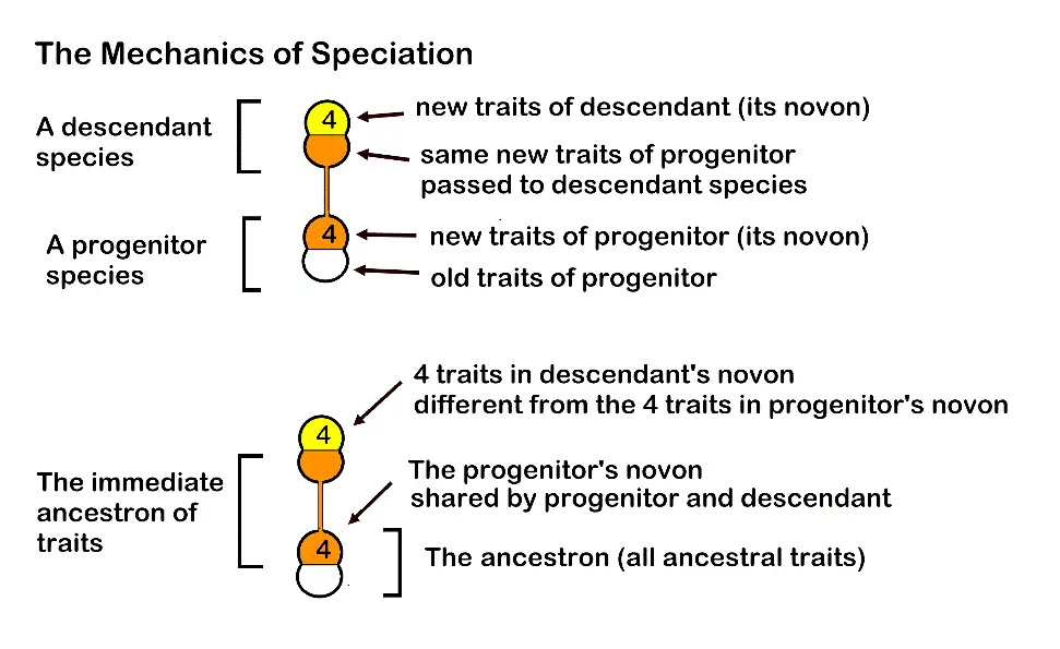
Figure 1. Details of optimized trait-sharing during speciation. An average of four traits is expected.
3.3. The Rule of Four
Past work has dealt with more than twenty-five minimally monophyletic groups [1], and, significantly, the average number of descendant species per ancestor is about four in recently evolved groups not yet subject to much extinction. Also, the number of traits that are newly evolved (generated and fixed in speciation) is about four. Apparently, a Rule of Four [19] involving four as an optimizing factor is present in many fields [20,21,22]. In evolutionary taxonomy, this implies a quadratic fractal process [23,24,25,26] where four is an optimal number that applies across scales. At first, this appeared to be due to crowding [22,27], but it is more probably due to Bayesian exclusion of two-sigma of uncertainty (as discussed below).
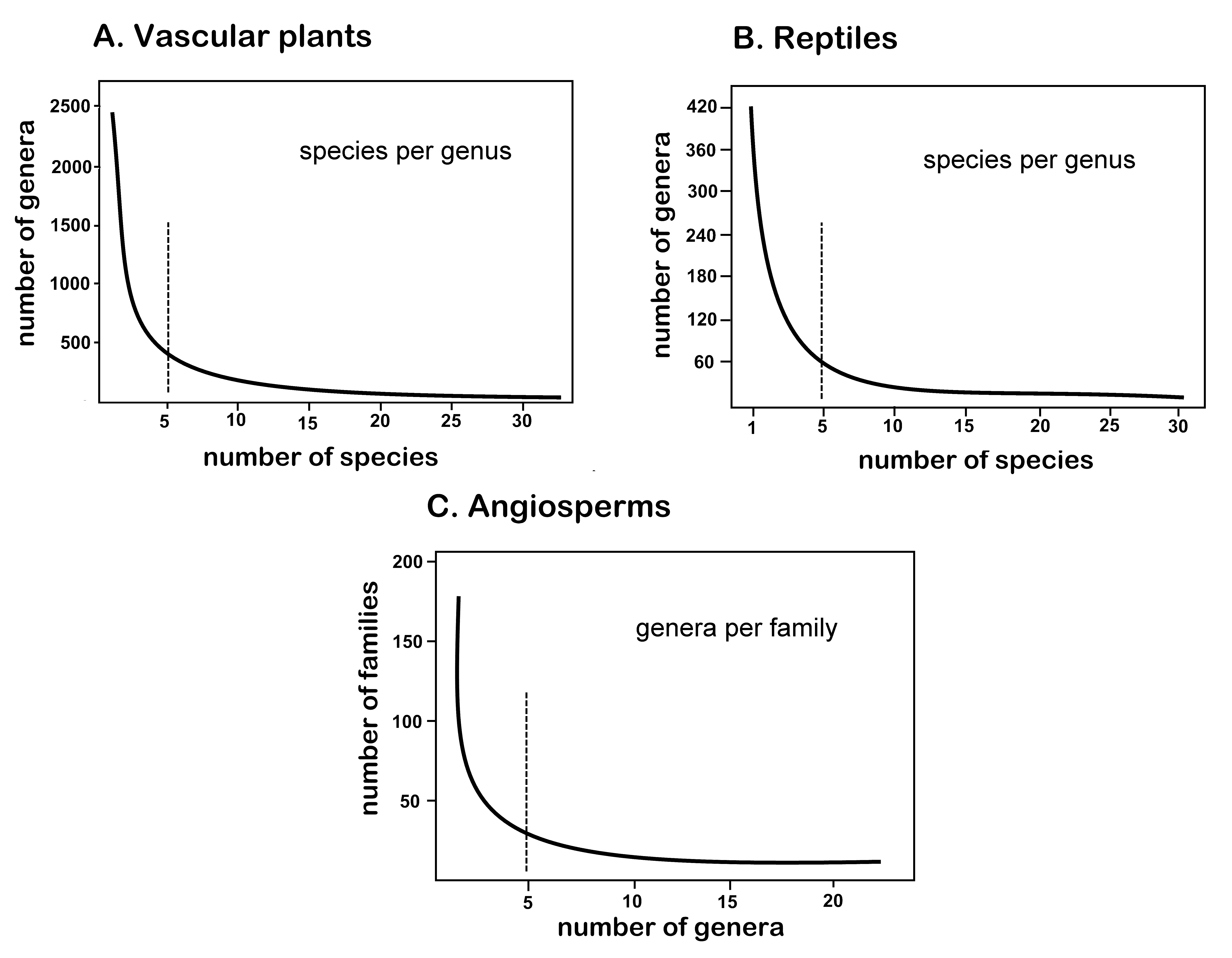
Figure 2. Inverse function graphs or “hollow curves”. (A) Vascular plant species per genus. (B) Reptile species per genus. (C) Angiosperm genera per family, reflecting self-similarity across scale.
The optimal number of species per genus seems to be about 4. Analysis, given time available for revisionary analysis, has stopped (by publishing) at (1) one large genus of 23 species (Leptodontium) split into 10 MMGs [1], (2) three MMGs obtained by resurrection from a larger molecular genus that combined them [28], and (3) 15 other genera of smaller size that proved to be MMGs simply awaiting dissection into progenitor and descendant species [1]. Very large genera like the moss Syntrichia [29] and Didymodon [30] have not been well studied, but are probably either large undistinguished sets of MMGs or obey a different emergent fractal process [31,32], perhaps involving powers of two or four. The large moss genus Chionoloma, however, is a composite of several minimally monophyletic genera [28]. Given the range and number of minimally monophyletic taxa studied, it is thought sufficient to make broadly predictive hypotheses applicable to the large number of already small classical genera, pending work on larger genera.
To be avoided is the multiplication of traits through supervenience, which is the recognition of traits that are not causative. For instance, what are apparently three traits, increase in length, width and depth, may be one trait, an increase in volume. In addition, there may be important traits in addition to the morphological, including those of physiology, ecology, geography, chromosome counts, chemistry, and genomics. However, each of these topics is at a different scale, and, as with the scales of the taxonomic hierarchy, one might expect self-similar numbers of traits at each scale, something definitely worth investigating.
Since graphs of genera per family also exhibit about the same inverse function [33,34], a fractal process may be involved with one generative element (the progenitor) and about four products of speciation (the immediate descendants). The published inverse functions generally follow Equation (1), where the power of the denominator is the fractal dimension of ln 5/ln 4. The fractal dimension describes the common speciation outcome that one ancestor generates about four descendant species; in that all five species share the same novon of the ancestor, generation of five from four is a fractal dimension of ln 5/ln 4, or 1.161.
3.4. Taxonomic Study
There are major differences between this method and that of modern cladistics, but the most important is familiarity with the morphological traits of species, which requires taxonomic expertise developed through revisionary work. Happily, taxonomy [35] builds on 250 years of the work of others, and in most groups of organisms the species are at least preliminarily sorted by overall similarity. This sorting eliminates a great deal of the homoplasy (convergent traits) in morphological data sets by making the data sets hierarchically smaller. So small, in fact, that most newly evolved genera are already between 1 and 5 species in size [15]. For revision, the standard dichotomous key, which sorts species names into couplets, is sufficient and helps distinguish smaller sets of species within larger genera. One must be aware, however, that distinctive species are often “taken out” at the start of dichotomous trees to simplify quick identification, and are not necessarily associated with related, less prepossessing species. In addition, fully dichotomous sorting is sufficiently ingrained in taxonomic methodology that it biases the construction of evolutionary trees such that complete dichotomy is viewed as “fully resolved”, as a stopping rule, ignoring the potential of multiple descendant species from one progenitor.
3.5. Polychotomous Phyletic Key and Minimally Monophyletic Groups
The idea is to recognize minimally monophyletic groups that differ internally by only a few traits between ancestral and descendant species. Identification keys are generally valuable for digesting lengthy descriptions of organisms into the few traits that best distinguish any one species from similar species. A phyletic key requires the recognition of evolutionary relationships and often relies on technical characters. It differs from a standard key in diagraming evolutionary relationships by small or at least parsimonious increments in trait changes. Generalist species are placed at the beginning of the phyletic key and the most specialized at the end, the opposite of standard dichotomous keys, which differ in commonly identify the least specialized species as that which is left after easily distinguished species are identified. The small size of the minimally monophyletic group (MMG) helps instigate the inferential method of using a second-order Markov chain. For this, two items of data are required to establish placement in a phyletic key. The genus ancestral species is that which is (1) most similar to some outgroup species (which may or may not be its own ancestor), and also (2) is most generalist to the ingroup of more specialized species. This is a straightforward simplex-convex situation. Given that, when developing a phyletic key, one ancestral species does commonly generate more than one descendant species, a true phyletic key is necessarily polychotomous.
3.6. Second Order Markov Chain
The criteria for polarization of trait changes are many. Polarizations provide considerable support for a decision in high-resolution phylogenetics because they build sequentially a caulogram by two comparisons (the one species with most similarity to an outgoup, and also most generalized towards ingroup) for determining the identify of a progenitor of multiple descendants. Every MMG has distinctive polarizations of traits involved in its structure. Some polarizations used in revision of the MMGs of this paper include: (1) reduction in size or organ expression; (2) no reversals; (3) parsimony of trait changes; (4) specialization or elaboration; (5) asexual reproduction; (6) precinctiveness or adaptation to small niches or patches; (7) recency of geologic area; (8) isolation of range or geography; (9) chromosome number change; (10) apophyly-paraphyly in molecular analyses; (11) major distance on a molecular cladogram; and (12) rarity of traits. The stopping rule must be the point at which additional traits add little to the resolution of a caulogram, particularly redundant traits that come from different scales when analysis requires total evidence.
3.7. Generation of a Caulogram
A cladogram is simply a standard dichotomous key to species rendered in large part phyletic by cluster analysis of trait changes. The dichotomous nature of an identification key is ingrained in the practice of taxonomy as immensely useful, but is inappropriate for evolutionary resolution of multiple descendant species generated by a single progenitor, even if the progenitor mutates in DNA without a significant change in taxonomically important expressed traits. Expressed traits are the working substance of evolutionary change.
A polychotomous phyletic key is essential to estimating structural monophyly at the microgenus level because this is the first step in how an MMG is distinguished. A microgenus is defined as one progenitor plus its immediate descendant species, each species of the genus sharing the newest traits of the progenitor. The MMG governs how survival-based traits are preserved and shared. A species in ancestor-descendant analysis may have any definition that works within the definition of a microgenus.
The MMGs are concatenated into a larger multi-genus evolutionary tree with much the same criteria. The progenitors of the microgenera (individual phyletic keys) are connected with other progenitors of microgenera by the smallest number of trait changes. Inferentially, this is simple parsimony extended from intra-genus to inter-genus. The caulogram may be a branching dendrogram with names of extant (or rarely inferred extinct) species assigned to the nodes, or it can take the form of a spreadsheet with data embedded in arranged cells. A study of species in the West Indies [22] shows clear evidence of the generation of four descendant species from one ancestral species (Figure 3).
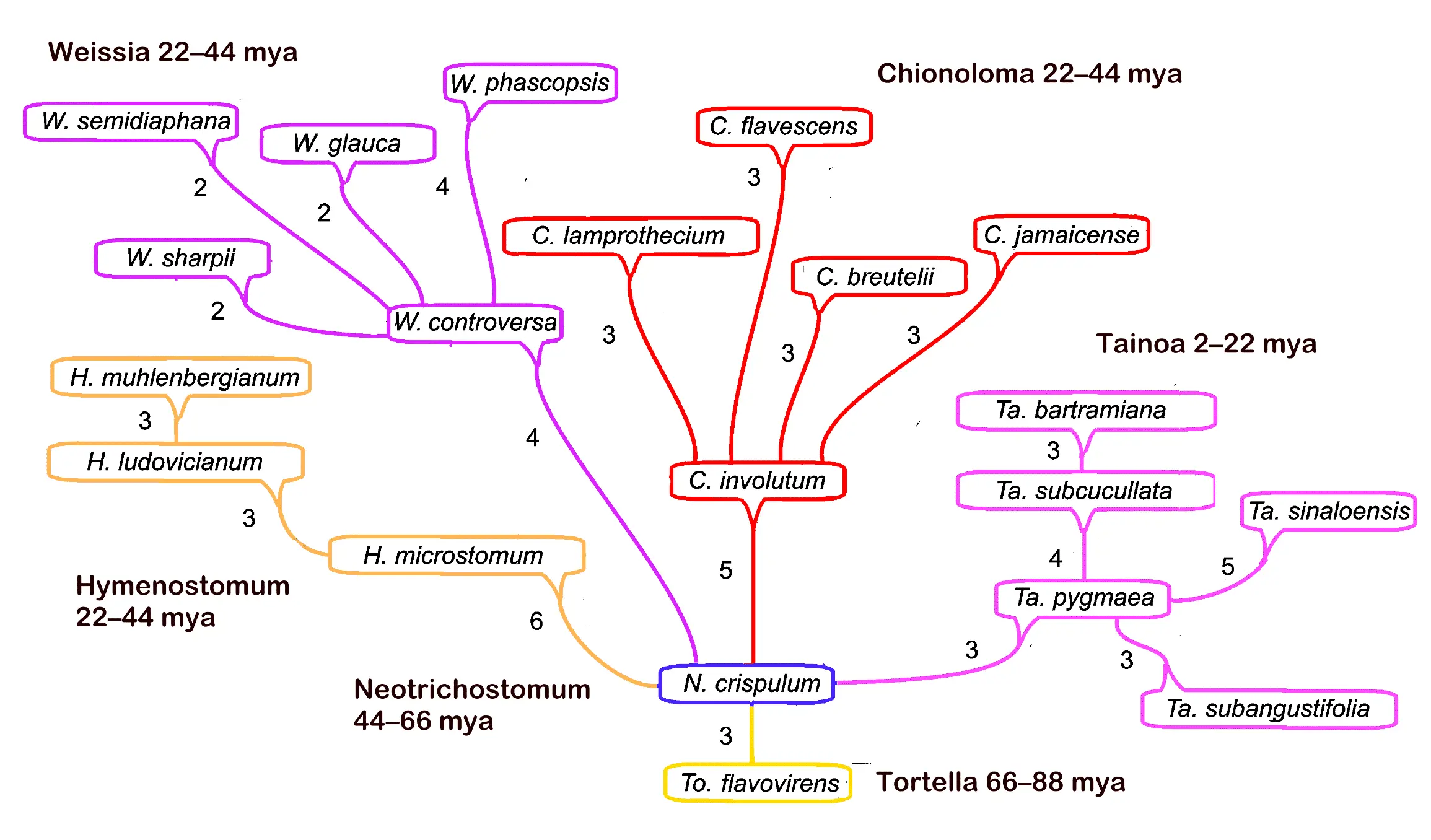
Figure 3. Example of a caulogram, showing speciation patterns through 88 million years for a set of genera now largely in the West Indies. Numbers of new traits per speciation event are given. Adding them sequentially from the caulogram base provides Shannon bit totals interpreted as Bayesian posterior probabilities. Stopping rule is full polychotomous resolution, as above.
3.8. Shannon-Turing Sequential Bayes
Morphological cladistics has had a bum rap because of the misuse of nonparametric bootstrapping [36] as a method of evaluating consistency and robustness of the data. Cladistic studies rely on large data sets, which in cladistic systematics are evaluated with various optimization methods to determine common ancestry. Parsimony is a basic method, but the use of molecular data has created a cottage industry in complex statistical methods [37], such as coalescent Bayesian Markov chain Monte Carlo. Non-parametric bootstrapping with morphological data is essentially resampling with replacement, a common statistical practice. Because the data sets for morphology are generated from descriptions of species, however, deletion of data for resampling eliminates major features of the species. A species description is a distillation of multiple samples, and the correct application of bootstrapping would be resampling among descriptions of specimens, not species. Resampling descriptions of multiple specimens would strongly support the consistency and robustness of morphological descriptions. To obviate this long-ingrained bias against using morphology in evolutionary systematics, a new method called Shannon-Turing sequential Bayesian analysis [1] is used, which generates posterior Bayesian probabilities for a caulogram structure as high as those for cladograms from molecular analysis.
The method is to assign one Shannon informational bit to each new trait of a newly evolved species. Because bits are logarithmic (base two), they are additive. An odds table (Table 1) provides the Bayesian posterior probabilities [38]. The bits can be added along any short or long stretch of a caulogram, providing support for any number of concatenated species in a lineage. Positioning species on a dendrogram such that there is a minimum or absence of reversals avoids negative bit values, a kind of parsimony. Given the small size of minimally monophyletic groups, the mathematics is straightforward. Conjugate priors can be calculated such that probabilistic support for and against a particular caulogram structure can add to probability 1.00, but this is generally not necessary. Secondary descent (one descendant being ancestor to one other descendant) is treated statistically separately as a separate process, as an inchoate or remnant minimally monophyletic group, which avoids normalization in calculating conjugate priors.
Because morpho-species are already arranged taxonomically in hierarchically nested groups, large data sets are unnecessary for Shannon-Turing analysis (Figure 4). This built-in stopping rule consists of the critical traits involved in speciation being clearly set out when a small, minimally monophyletic group is evaluated for ancestor-descendant relationships. Generally, only three to five traits are involved among those possible character states identified in prior taxonomic studies. The model of evolution in MMGs may be better understood as a simplex-convex model, an analytic technique not yet formally pursued.
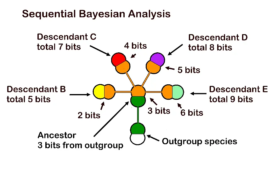
Figure 4. Bayesian support in one genus through assignment of one Shannon bit for each new trait in a speciation event, then adding them to get Bayesian posterior probabilities. The genus comprises one ancestral species and four immediate descendants, where orange denotes the shared immediate ancestral trait set. In this contrived example, the ancestor has 3 new traits (its difference from the outgroup species), which are added to the new traits of each descendant to get total bits for the odds table and calculation of the Bayesian posterior probability. Support for the topology of the whole genus is 3 + 5 + 7 + 8 + 9 bits or 32 bits, a very high Bayesian support measure.
Below is a polychotomous phyletic key [28] for the pottiaceous moss genus Pseudosymblepharis. The indentations represent one or more speciation events from one ancestral species. Thus, P. angustata has three descendant species. A new trait is a bit; the odds table (Table 1) gives sequential Bayesian posterior probability [38] as the bits are added along the lineage. Information in this which is essentially a caulogram in sentences, includes a number of novel traits in the speciation event, species name, number of bits in the speciation event, plus that of the previous speciation event used to calculate sequential Bayesian posterior probability (SBPP).
1. Three traits: Neotrichostomum crispulum, 3 bits, SBPP 0.89.
2. Seven traits: Pseudosymblepharis subduriuscula, 3 + 7 bits, 0.999 SBPP.
3. Two traits: P. burneense, 7 + 2 bits, 0.998 SBPP.
2. Four traits, P. angustata, 7 + 7 bits, 0.999 SBPP.
4. Three traits P.dubia, 4 + 3 bits, 0.992 SBPP.
4. Two traits, P. orthodonta, 4 + 2 bits, 0.985 SBPP.
4. Two traits, P. richardsii, 4 + 2 bits, 0.985.
2. Five traits, P. schlimii, 7 + 5 bits, 0.9998 SBPP.
5. Two traits, P. circinata, 7 + 2 bits, 0.998 SBPP.
5. Three traits, 7 + 3 bits., 0.999 SBPP.
Table 1. Odds converted to Bayesian posteriors. Shannon’s informational bits at one per new trait are directly translatable into support probability. Each bit is given its value as a power of two, the odds ratio as a proportion of value to 1, the odds ratio presented as a fraction, and the percent probability or Bayesian posterior probability of that fraction. Bits may be added to derive a sequential Bayesian posterior probability (SBPP).
|
Bits |
0 |
1 |
2 |
3 |
4 |
5 |
6 |
7 |
8 |
|---|---|---|---|---|---|---|---|---|---|
|
Value |
1.00 |
2.00 |
4.00 |
8.00 |
16.00 |
32.00 |
64.00 |
128.00 |
256.00 |
|
Odds ratio |
1:1 |
2:1 |
4:1 |
8:1 |
16:1 |
32:1 |
64:1 |
128:1 |
256:1 |
|
Fraction |
1/2 |
2/3 |
4/5 |
8/9 |
16/17 |
32/33 |
64/65 |
128/129 |
256/257 |
|
Probability |
0.500 |
0.667 |
0.800 |
0.889 |
0.941 |
0.970 |
0.985 |
0.992 |
0.996 |
|
Bits |
9 |
10 |
11 |
12 |
13 |
14 |
|||
|
Odds ratio |
512:1 |
1024:1 |
2048:1 |
4048:1 |
8096:1 |
16192:1 |
|||
|
Fraction |
512/513 |
1024/1024 |
2048/2049 |
4048/4049 |
8096/8097 |
16192/16193 |
|||
|
Probability |
0.99805 |
0.99902 |
0.9995 |
0.99975 |
0.999876 |
0.999938 |
|||
3.9. Two-Sigma Structural Monophyly
The average number of immediate descendants in a minimally monophyletic groups is about four. According to the odds chart (Table 1), four Shannon bits is about 0.941 Bayesian posterior probability. This excludes about two standard deviations (two sigma) of uncertainty. The same holds true for the average number of traits in a species. This value matches the inflexion point of a bell-shaped (Gaussian) curve and is not arbitrary. The process of excluding about 95% of uncertainty is apparently almost universal [39] in evolutionary processes, particularly those reflecting the Pareto ratio, which is involved in the fractal dimension of evolution [22]. The broader implications of a widespread two-sigma exclusionary process will be discussed in a future paper. Selection-mediated exclusion of two-sigma of uncertainty may generate and sustain biodiversity. When established for a taxon, it would provide a strong stopping rule for evolutionary taxonomy. That which is measured as uncertainty is the failure of individuation (survival as a taxon) due to too few traits per species (or species per genus) or lumbering adaptability with too many new traits.
3.10. Evolutionary Trends and Geologic Time Depth
The traits that are newly evolved in speciation are associated with and identify adaptive trends in evolution [40]. This is as opposed to morphological traits that are only mapped on molecular trees generated with common ancestry analysis. Although parsimony is clearly involved in evaluating an MMG, it is done in the context of descent with modification, not common ancestry, and as an optimizing criterion: the most parsimonious MMG is a direct model of expressed traits evolution. Evolutionary trends, that is, traits associated with particular niches or environmental changes, can be confidently ascribed to microgenera. For example, in the moss family Streptotrichaceae, the microgenus Crassileptodontium is clearly adapted to volcanic substrates, while Stephanoleptodontium is strongly associated with both soil and humus at high elevations in the tropics, while the most primitive (first) of extant progenitors, Streptotrichum and its sibling genus, Trachyodontium, are both arboreal [1]. The hypothesis that early genera of the family Streptotrichaceae survived extinction events while living on tree branches is then directly supported, rather than mediated by molecular tracking. Ideally, a molecular study of apophyly and paraphyly should be done to confirm or clarify the morphological results, but the data are as yet unavailable. The strong statistical support for the Streptotrichaceae caulogram [1] implies that predictions regarding evolutionary trends are justified.
That which descends is the set of proven traits of the immediate ancestron, while that which is modified are older traits less important for immediate survival. Conclusions are that one large group of minimally monophyletic genera (Streptotrichaceae of 10 extant genera plus 3 inferred as extinct) is very old in origin, reaching back to the late Cretaceous, while a similarly large group (Pleuroweisieae of 11 extant genera) apparently reach back only to the Paleocene-Eocene era. The range of geological age is correlated with the stability of habitat, and otherwise with exposure to catastrophic environmental change. Estimated geological time is given in Figure 3 for the Neotrichostomum group in the West Indies [22], and in Figure 5 for the family Streptotrichaceae.
The stopping rule for speciation pace in geologic time relies on three criteria: (1) fossil anchoring species of similar morphology, (2) the confinement of one genus of five species to a recent (46 my) land mass, the West Indies, and (3) similar distributions of similar-sized taxonomic groups of similar morphology across the same geologic time scale. The stopping rule is pre-determined by the previous success in using anchoring fossils and an assumed molecular clock, while a new criterion is the dating of available geographic substrate that allows a morphological clock matching to a large extent a molecular clock [28].
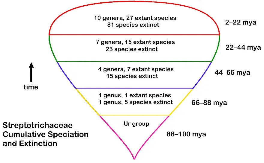
Figure 5. Summary of progress of extinction and speciation inferred for the bryophyte family Streptotrichaceae over 100 million years, as an example of high-resolution phylogenetics.
3.11. Evolutionary Distance, Momentum and Force
A paper [2] has been recently published expressing modes and tempo of evolution in terms of classical mechanics. The number of trait changes is equivalent to evolutionary distance, the expressed character set of any one species is mass, momentum is distance times mass, and force is acceleration times mass. By equating force with evolutionary resilience to environmental change, each microgenus may be assigned a measure of success in sustainability over geologic time scales. In this study, the innovation is that by adding all new trait changes along a caulon (a single line of stem-taxon species from base to species), one can place a comparative measure on acceleration. If the mass is considered the number of species in the caulon (adding all progenitors in a line), then force, as acceleration times mass, is easily calculated. The stopping rule is the ability to make comparisons between species, genera, and higher taxa in regard to their differential evolutionary resilience with similar results in two different bryophyte lineages, the family Streptotrichaceae and Pottiaceae trube Pleuroweisieae (Figure 6).
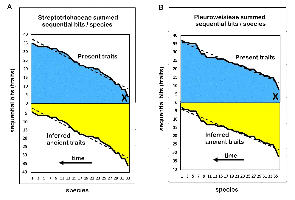
Figure 6. Summed trait changes in a caulogram lineage per species equate to force in classical mechanics, interpretable as resilience to environmental change. (A) Streptorichaceae. (B) Pleuroweisieae. In both diagrams, increasing numbers of extant, adaptive traits over time (blue) imply a parallel decrease in extinct, ancient traits now unused (yellow). The dashed line is an Excel software (version 2509) linear trendline. X marks the most ancient surviving species.
3.12. Redundancy
The fact that a progenitor shares its most recent traits with all immediate descendant species imbues the microgenus a redundancy of traits. That is, in a microgenus, all species share an identical set of ancestral traits. Such redundancy has evolutionary importance [41] in providing flexibility in a group. The redundancy of traits in microgenera can be expressed as probabilistic information, this in terms of Shannon entropy [5,42]. Redundancy is calculated with Shannon methods [4], where maximum entropy minus Shannon entropy divided by maximum entropy as a normalizing function yields a redundancy measure.
A comparison of these measurements in more than 20 microgenera [5] demonstrated that these values were all very similar across all microgenera. A portion of the spreadsheet is given here in Table 2. The implication is that a natural process, probably natural selection, has fixed the level of trait redundancy to be similar in all MMGs. A lineage is optimized for survival by natural selection and descent with modification and, through redundancy has a self-correcting structure. The stopping rule is that the same large number of sampled species have trait composition that allows predictive hypotheses to be extended to other small genera and perhaps to other large genera that are potentially able to be dissected into MMGs.
Table 2. Example of redundancy calculation for a minimally monophyletic genus Ardeuma in Pottiaceae tribe Pleuroweisieae. Evolutionary tree (caulogram) in spreadsheet implementation (the angled arrows), total traits important in speciation, and maximum entropy, Shannon entropy, and entropic redundancy are given.
|
Genus |
Species |
New Taits |
Total Evol. Traits |
Max. Entropy, Shannon Entropy, Redundancy |
||
|---|---|---|---|---|---|---|
|
Ardeuma |
gracillimum |
4 |
4 |
|||
|
recurvirostrum |
╚> |
2 |
4 + 2 |
|||
|
crassinervium |
╠> |
3 |
4 + 3 |
|||
|
annotinum |
╠> |
3 |
4 + 3 |
|||
|
aurantiacum |
╚> |
3 |
4 + 3 |
|||
|
Total |
31 |
4.95, 3.46, 0.30 |
||||
4. Discussion
4.1. Comparison with Cladistic Methodology
High-resolution phylogenetics is a form of numerical taxonomy that melds classical evolutionary taxonomy with molecular systematics and reaffirms the importance of standard taxonomic methods. Polychotomous and multiorder Markov chains are more consonant with evolutionary theory than a cladogram’s dichotomous and first-order Markov chain. Standard practice for taxonomically evaluating variation in a species, short of fully fledged statistical analysis, is to continue sampling and not halt until there is no change; that is, the range of states is established, given reasonable effort and an expectation that most species are not entirely stenomorphic. This is not done in molecular analysis, which no longer has the excuse of DNA sampling being too expensive. The variable that is critical for high-resolution evolutionary analysis is not that which tracks shared ancestry, but that which reveals apomorphy-paraphyly polarizations. Following is a numbered list of the more salient criticisms of cladistic phylogenetics.
- (1)
- The present analysis uses a descent with modification model rather than shared ancestry. It uses extant ancestral species at nodes in a multiple-branching tree related by a small number of traits modeled by a second order Markov chain, in which the ancestor is identified as a generalist with respect to the descendants and also as most similar to the outgroup. Cladistic analysis models evolutionary trees without designating any extant species as ancestral. In Figure 7, A and D are not identified cladistically as either ancestral or descendant, but are revealed as such in the caulogram. Van Valen [43] long ago pointed out that there are many species that are clearly ancestral to other species. My own analyses indicate that about half the species involved in any large-scale study are progenitors of at least one of the other species [1]. Molecular analyses do not identify extant shared ancestors as such.
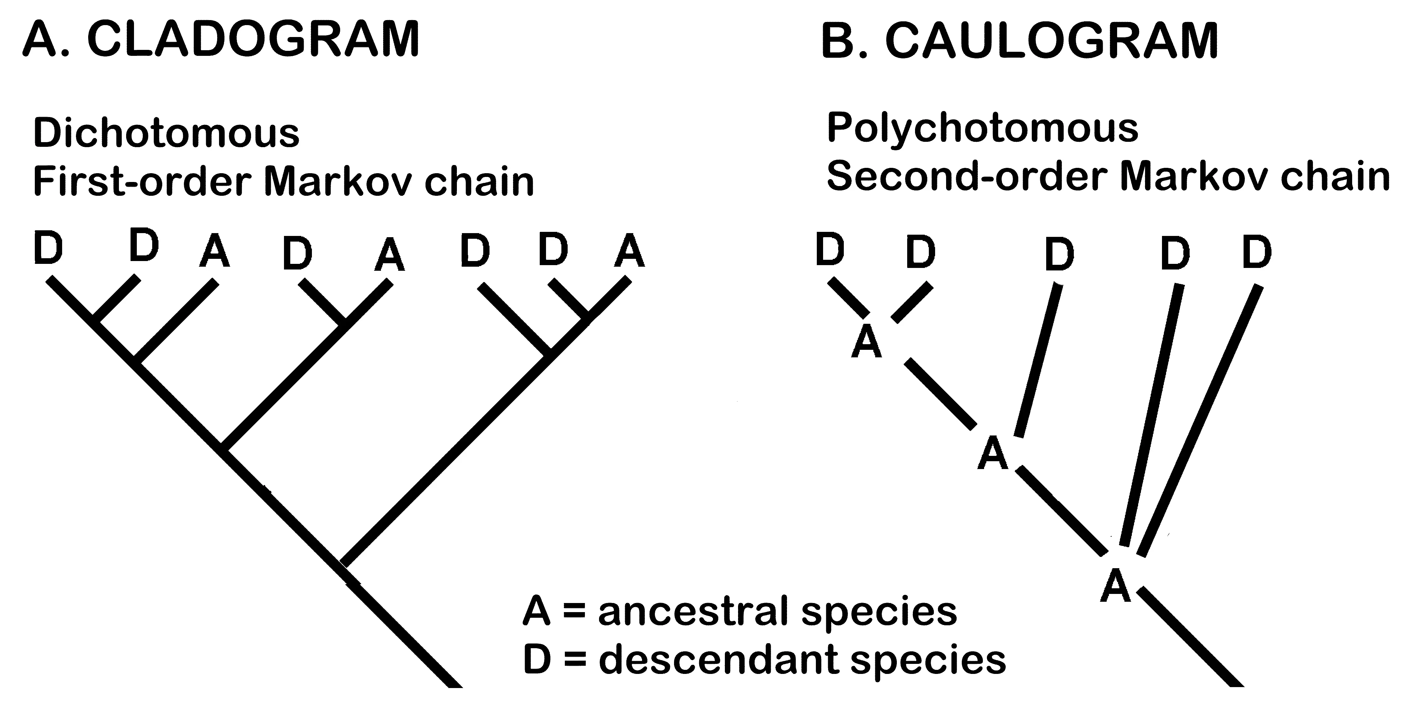
Figure 7. Comparison of cladogram and caulogram. (A) The cladogram (left) is based on the estimation of common ancestry of the terminal taxa (letters A and D). (B) The caulogram (right) is based on descent with modification, where A is clearly a progenitor of one or more species and D are immediate descendant species.
- (2)
- There may be still living molecular strains of an ancestral species with phylogenetically informative sequences identical to each descendant species (Figure 8). Because there are optimally about four descendant species from one ancestral species, sampling only one of these ancestral molecular doppelgangers gives a clade only a 20% chance of being monophyletic. That molecular strain may be identical to any one of the four descendant species. When sampling is sufficient to identify molecular doppelgangers, the bracketing of apophyly-paraphyly pairs helps to identify descendant-ancestral species pairs. Adequate data for identifying apophyly-paraphyly pairs are rare in published sparsely sampled molecular cladograms. The distance between doppelgangers on a molecular cladogram [1] is in line with and supportive of the estimate of an optimal four morpho-descendants per morpho-progenitor. The more recent molecular variants should tend to be sampled more often than the more ancient and should be more likely to appear terminally or near terminally on a cladogram with their molecular descendant species.
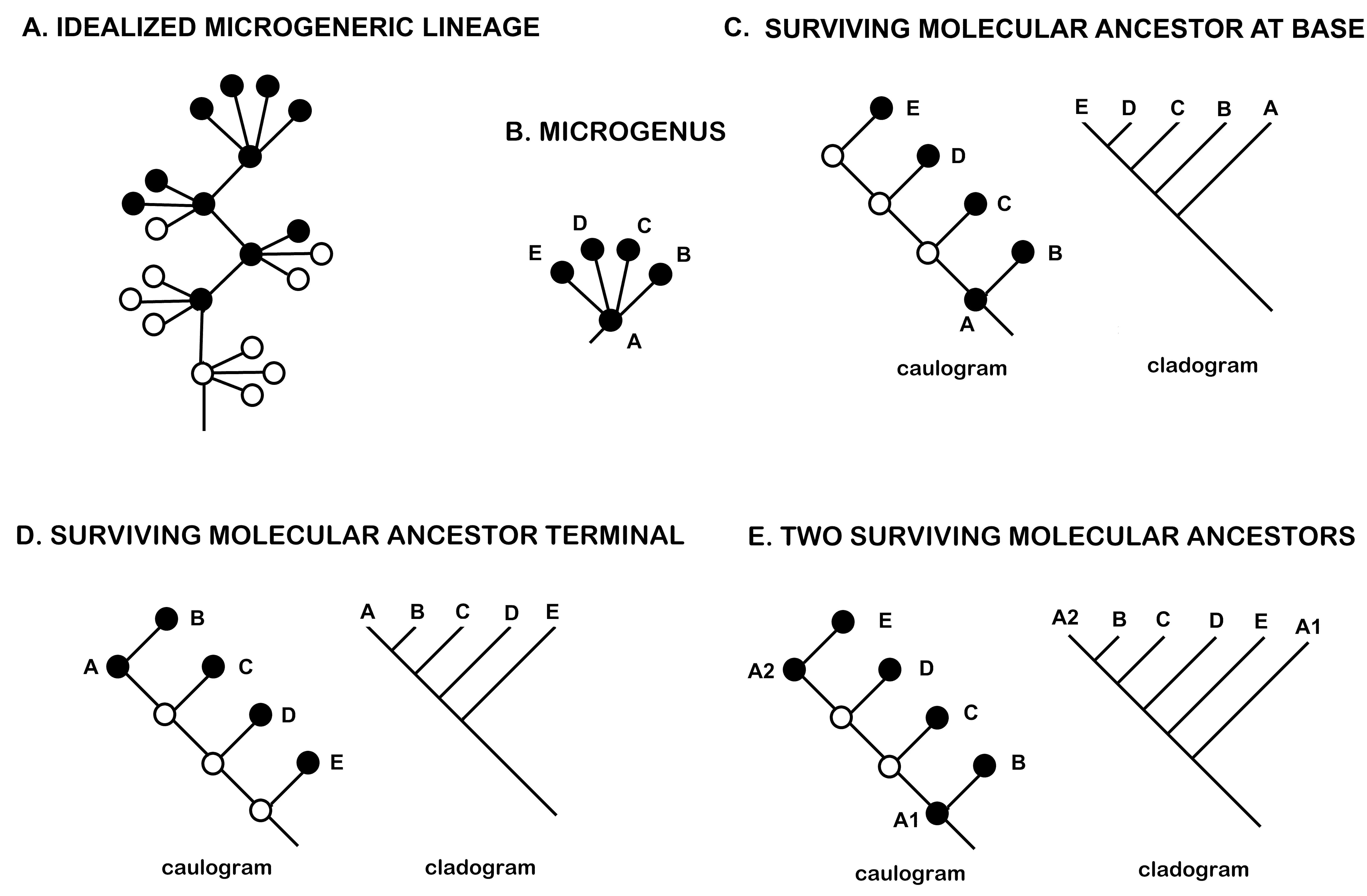
Figure 8. Problematic molecular data. (A) Four microgenera in a lineage, extant species are solid dots, extinct are circles. (B) Idealized new microgenus with four immediate descendant species. (C) Caulogram and equivalent cladogram with surviving ancestral molecular variant at base. (D) Same but surviving ancestral molecular is terminal. (E) Same, but there are two surviving molecular variants, A1 and A2, resulting in informative paraphyly (B, C, D, and E must descend from morphospecies A).
- (3)
-
Using descent with modification as an analytical method involves recognition of minimally monophyletic groups and more exact modeling of shared ancestry. Taxonomic categories of species and genus are critical in evolutionary analysis [44,45,46], while cladistics has no defensible concept of genus [47,48] or even species [49]. Some cladists [50] even deprecate “speciesism” as notional, without supportive evidence. Cladistics is not necessarily methodologically tied to evolution [51].
- (4)
-
Total evidence [52] requires comparison of models from both morphological and molecular data. Simply mapping morphological traits to a molecular tree avoids the realization that morphological data can produce statistically well-supported Bayesian trees that may differ from the molecular trees. The accuracy of second-order Markov chain analysis in determining extant ancestral species, in most cases, resolves monophyly well. Molecular cladograms can be wonderfully precise, but modeling evolution with morphological traits produces an informationally true and accurate tree. To achieve this, one must be familiar with the techniques of classical taxonomy and undertake examination of many samples [53,54,55] to establish the variability of data. This is opposed to relying on a few specimen samples and a black box of deeply complex statistical modeling, with a dichotomous tree concept dating back to phenotypic cluster analysis [56] that rejects the possibility of extant ancestral species.
- (5)
-
Structural monophyly postulates only a few extinct taxa, genera and species. These are apparently extinct taxa that serve to connect lineages, but the jump between genera requires over twice) The number of expected trait changes between two species. Cladists do not make such hypotheses, even as they postulate an unknown extinct shared ancestor for most species [57,58].
- (6)
-
Molecular analysis of evolutionary relationships initially focused on the use of DNA spacers and “junk” sequences, assuming that random mutations at a generally constant rate would allow the tracking of lineage as they split. Now it is clear that such sequences may contain many regulators and promoter codons, potentially increasing bias through environmental selection-driven convergence. The neutralist theory of evolution [11,58,59,60] in its strongest form postulates that new traits associated with speciation are generally randomly fixed. Apparently, this has given license to cladistics to use all molecular data, including coding genes, for systematic analysis.
Against such practice, a recent analysis of the plastome of the genus Tortula [61] has shown strong purifying selection in most genes, and positive selection in a smaller number, based on distribution of nonsynonymous-to-synonymous substitution ratios. A recent study of the large pottiaceous moss genus Syntrichia [29] used 354 nuclear exons for each of 79 species. The resulting molecular cladogram placed many species into ecologically similar groups. An appraisal of one of the terminal groups of several arboreal species showed no morphologically based structural monophyly, that is, no simple arrangements of closely related species in small groups that might be interpreted as minimally monophyletic. The use of exons is ill-advised due to the probability of massive bias due to convergence.
4.2. Protocol for High-Resolution Phylogenetics
Given the above caveats and possible problems, a simplified set of steps for the structural monophyly analysis is given below:
- (1)
-
Spreadsheet the morphological information.
- (3)
-
Create a polychotomous phyletic key (e.g., Table 1).
- (3)
-
Create a caulogram from the above key (e.g., Figure 4), showing ancestral species and a few direct descendant species with a few secondary descendants. The caulons (connections from the base to terminal taxa) are inferred between the ancestors of species, occasionally with interspersions of secondary descendants.
- (4)
-
Use maximum parsimony to find minimal trait changes between the few species in a minimally monophyletic group. This is simple math with only a few species to deal with, each with a few novel traits.
- (5)
-
Expect quadratic patterns of descent with ca. 5 species per recent genus.
- (6)
-
Use Shannon-Turing analysis and a second-order Markov chain to estimate support for each ancestor-species pair.
- (7)
-
Compare caulograms of different large taxa by evolutionary distance, velocity, momentum, and force to evaluate differential resilience and stability (e.g., Figure 5).
- (8)
-
Formally name and describe MMGs as nomenclaturally active genera (here called “microgenera”).
- (9)
-
Formally name and describe the set of concatenated MMGs as suprageneric taxa (tribes, subfamilies, families).
- (10)
-
Evaluate depth in evolutionary or geologic time using fossil anchors and estimates of recent genus establishment in recently established large habitats, environments or localities (e.g., Figure 6).
5. Conclusions
The aim of high-resolution phylogenetics using morphology in evaluating structural monophyly is to identify and clarify the processes of evolution that have led to present-day robust, long-term, resilient biological lineages that support shared ecosystems. Biodiversity is generated and stabilized by the minimally monophyletic group in its sharing of the new traits of the ancestral species with all its immediate descendants, and the quadratic restriction of numbers of descendant species, apparently important at all scales, given self-similarity [62] at genus and family levels.
It may be suggested that genera provide the low Shannon entropy of the immediate ancestron’s massive redundancy, supporting survival of descendant species in present-day environments. This is while higher level taxonomic groups of tribes, subfamilies, and families each present a bank of survival-tested character states in their character sets, of which one of each character state is active and expressed somewhere in the lineage for immediate adaptive action on behalf of the lineage during environmental change, while the remaining potential character states are available for more longer selection and fixation processes. Thus, genera are well-equipped to survive locally in space and time, while the lineage of several to many minimally monophyletic groups holds the keys to long-term survival of the entire assemblage, including an unexpectedly fast rate of evolution in response to rapid environmental change.
The stopping rules for structural monophyly analysis require thorough analysis of variation in both morphology and molecular sequences, identification of the basic minimally monophyletic group using second-order Markov reasoning, a matching of morphological and molecular information on ancestor-descendant relationships (apophyly-paraphyly), and high statistical support for both morphological and molecular hypotheses of descent with modification, through matching analyses of total evidence.
If the original pre-determined stopping rule for evolutionary analysis is to generate a well-supported evolutionary tree using total evidence, then cladistics stops too soon. The original stopping rule is simply abandoned in favor of a molecular-only ultrametric or phyletic cladogram where polychotomies are deprecated as “unresolved”. The existence of an alternative method that more accurately reflects the aims of a reasonable stopping rule should encourage an abandonment of molecular-only cladistic cluster analysis and the mapping of morphological traits to molecular cladograms.
Statement of the Use of Generative AI and AI-Assisted Technologies in the Writing Process
During the preparation of this manuscript, the author used Gemini/Google for literature searches. After using this tool/service, the author reviewed and edited the content as needed and takes full responsibility for the content of the published article.
Acknowledgments
The author is grateful to the Missouri Botanical Garden for its continued support of novel research in plant systematics.
Ethics Statement
Not applicable.
Informed Consent Statement
Not applicable.
Data Availability Statement
All relevant data are included in the article.
Funding
This research received no external funding.
Declaration of Competing Interest
The author declares that he has no known competing financial interests or personal relationships that could have appeared to influence the work reported in this paper.
References
-
Zander RH. Structural Monophyly Abstractions. Res Botanica Technical Report 2025-09-30. Available online: https://www.researchgate.net/publication/396167046_Structural_Monophyly_Abstractions (accessed on 4 December 2025). [Google Scholar]
-
Zander RH. Biodiversity resilience in terms of evolutionary mass, velocity and force. Sustainability 2025, 17, 8272. doi:10.3390/su17188272. [Google Scholar]
-
Morrison ML, Rosenberg NA. Mathematical bounds on Shannon entropy given the abundance of the ith most abundant taxon. J. Math. Biol. 2023, 87, 76. doi:10.1007/s00285-023-01997-3. [Google Scholar]
-
Shannon CE. A mathematical theory of communication. Bell Syst. Tech. J. 1948, 27, 623–656. doi:10.1002/j.1538-7305.1948.tb00917.x. [Google Scholar]
-
Zander RH. Shannon entropy and informational redundancy in minimally monophyletic bryophyte genera. Plants 2025, 14, 3066. doi:10.3390/plants14193066. [Google Scholar]
-
Brooks DR, Wiley EO. Evolution as Entropy: Toward a Unified Theory of Biology; University of Chicago Press: Chicago, IL, USA, 1988. [Google Scholar]
-
Weber BH, Depew DJ, Smith JD. (Eds.) Entropy, Information and Evolution; MIT Press: Cambridge, MA, USA, 1990. [Google Scholar]
-
Fletcher SC. The stopping rule principle and confirmational reliability. J. Gen. Philos. Sci. 2024, 55, 1–28. doi:10.1007/s10838-023-09645-6. [Google Scholar]
-
Mitchell L, Polansky L, Newman KB. Stopping rule sampling to monitor and protect endangered species. J. Agric. Biol. Environ. Stat. 2024, 1–19. doi:10.1007/s13253-024-00649-3. [Google Scholar]
-
Rouder JN. Optional stopping: No problem for Bayesians. Psychon Bull. Rev. 2014, 21, 301–308. doi:10.3758/s13423-014-0595-4. [Google Scholar]
-
Nei M, Kumar S. Molecular Evolution and Phylogenetics; Oxford University Press: New York, NY, USA, 2000. [Google Scholar]
-
Uyeda JC, Zenil-Ferguson R, Pennell MW. Rethinking phylogenetic comparative methods. Syst. Biol. 2018, 67, 1091–1109. doi:10.1093/sysbio/syy031. [Google Scholar]
-
Darwin C. The Origin of Species by Means of Natural Selection, or the Preservation of Favoured Races in the Struggle for Life, 1963 Edition; Washington Square Press: New York, NY, USA, 1859. [Google Scholar]
-
Dayrat B. Ancestor-descendant relationships and the reconstruction of the Tree of Life. Paleobiology 2005, 31, 347–353. doi:10.1666/0094-8373(2005)031[0347:ARATRO]2.0.CO;2. [Google Scholar]
-
Willis JC. Age and Area; Cambridge University Press: Cambridge, UK, 1922. [Google Scholar]
-
Stevens PF. How to interpret botanical classifications: Suggestions from history. BioScience 1997, 47, 243–250. doi:10.2307/1313078. [Google Scholar]
-
François O. A multi-epoch model for the number of species within genera. Theor. Pop. Biol. 2020, 133, 97–103. doi:10.1016/j.tpb.2019.09.007. [Google Scholar]
-
Moonlight PW, Baldaszti L, Cardoso D, Elliott A, Särkinen T, Knapp S. Twenty years of big plant genera. Proc. R. Soc. B 2024, 291, 20240702. doi:10.1098/rspb.2024.0702. [Google Scholar]
-
Gazzarrini E, Cersonski RK, Bercx M, Adorf CS, Marzari N. The rule of four: Anomalous distributions in the stoichiometries of inorganic compounds. NPJ Comput. Mater. 2024, 10, 73. doi:10.1038/s41524-024-01248-z. [Google Scholar]
-
Constantin A, Bartlett D, Desmond H, Ferreira PG. Statistical patterns in the equations of physics and the emergence of a meta-law of nature. arXiv 2024, arXiv:2408.11065. [Google Scholar]
-
Wilkins A. The Laws of Physics Appear to Follow a Mysterious Mathematical Pattern. New Scientist, 21 October 2024. Available online: https://www.newscientist.com/article/2452341-the-laws-of-physics-appear-to-follow-a-mysterious-mathematical-pattern/ (accessed on 4 March 2025). [Google Scholar]
-
Zander RH. Fractal Evolution, Complexity and Systematics; Zetetic Publications: St. Louis, MI, USA, 2023; pp. 1–151. [Google Scholar]
-
Brown JH, Gupta VK, Li B-L, Milne BT, Restrepo C, West GB. The fractal nature of nature: Power laws, ecological complexity and biodiversity. Phil. Trans. R. Soc. Lond. B 2002, 357, 619–626. doi:10.1098/rstb.2001.0993. [Google Scholar]
-
Burlando B. The fractal geometry of evolution. J. Theor. Biol. 1993, 163, 161–172. doi:10.1006/jtbi.1993.1114. [Google Scholar]
-
Green DM. Chaos, fractals and nonlinear dynamics in evolution and phylogeny. Trends Ecol. Evol. 1991, 6, 333–337. doi:10.1016/0169-5347(91)90042-V. [Google Scholar]
-
Nottale L, Chaline J, Grou P. On the fractal structure of evolutionary trees. In Fractals in Biology and Medicine, Proceedings of the Third International Symposium, Ascona, Switzerand, 8–11 March 2000; Losa G, Merlini D, Nonnenmacher T, Weibel E, Eds.; Birkhauser: Basel, Switzerland, 2000; Volume 3, pp. 247–258. [Google Scholar]
-
Cressman R, Halloway A, McNickle GG, Apaloo J, Brown JS, Vincent TL. Unlimited niche packing in a Lotka-Volterra competition game. Theor. Popul. Biol. 2017, 116, 1–17. doi:10.1016/j.tpb.2017.04.003. [Google Scholar]
-
Zander RH. Integrative systematics with structural monophyly and ancestral signatures: Chionoloma (Bryophyta). Acad. Biol. 2024, 2, 1–14. doi:10.20935/AcadBiol7449. [Google Scholar]
-
Jauregui-Lazo J, Brinda JC, GoFlag Consortium, Mishler BD. The phylogeny of Syntrichia: An ecologically diverse clade of mosses with an origin in South America. Amer. J. Bot. 2023, 110, e16103. doi:10.1002/ajb2.16103. [Google Scholar]
-
Jiménez JA, Cano MJ, Guerra J. A multilocus phylogeny of the moss genus Didymodon and allied genera (Pottiaceae): Generic delimitations and their implications for systematics. J. Syst. Evol. 2021, 60, 281–304. doi: 10.1111/jse.12735. [Google Scholar]
-
Binning G. The fractal structure of evolution. Phys. D Nonlinear Phenom. 1989, 38, 32–36. doi:10.1016/0167-2789(89)90170-X. [Google Scholar]
-
Nicolis G, Prigogine I. Exploring Complexity: An Introduction; W.J.H. Freeman and Company: New York, NY, USA, 1989. [Google Scholar]
-
Linders GM, Louwerse MM. Zipf’s law revisited: Spoken dialog, linguistic units, parameters, and the principle of least effort. Psychon. Bull. Rev. 2022, 30, 77–101. doi:10.3758/s13423-022-02142-9. [Google Scholar]
-
Newman MEJ. Power laws, Pareto distributions and Zipf’s law. Contemp. Phys. 2005, 46, 323–351. doi:10.1080/00107510500052444. [Google Scholar]
-
Heywood VH. Principles of Plant Taxonomy; Van Nostrand: New York, NY, USA, 1983. [Google Scholar]
-
Felsenstein J. Confidence limits on phylogenies: An approach using the bootstrap. Evolution 1985, 39, 783–791. doi:10.1111/j.1558-5646.1985.tb00420.x. [Google Scholar]
-
Felsenstein J. Inferring Phylogenies; Sinauer Aoociates: Sunderland, MA, USA, 2004. [Google Scholar]
-
Pacrat D. Help Describing Decibans? LessWrong 2013. Available online: https://www.lesswrong.com/posts/hPR4jF8jJaQrJSyyZ/help-describing-decibans (accessed on 20 May 2021). [Google Scholar]
-
Mesarovic MD, Sreenath SN, Keene JD. Search for organizing principles: Understanding in systems biology. Syst. Biol. 2004, 1, 19–27. doi: 10.1049/sb:20045010. [Google Scholar]
-
Gingerich PD. Rates of evolution on the time scale of the evolutionary process. Genetica 2001, 112, 127–144. doi:10.1023/A:1013311015886. [Google Scholar]
-
Biggs CR, Yeager LA, Bolser DG, Bonsell C, Dichiera AM, Hou Z, et al. Does functional redundancy affect ecological stability and resilience? A review and meta-analysis. Ecosphere 2020, 11, e03184. doi:10.1002/ecs2.3184. [Google Scholar]
-
Harte J, Newman EA. Maximum information entropy, a foundation for ecological theory. Trends Ecol. Evol. 2014, 29, 384–389. doi:10.1016/j.tree.2014.04.009. [Google Scholar]
-
Van Valen L. A new evolutionary law. Evol. Theory 1973, 1, 1–30. [Google Scholar]
-
Barraclough TG. Evolving entities: Towards a unified framework for understanding diversity at the species and higher levels, Phil. Trans. Roy. Soc. B Biol. Sci. 2010, 365, 1801–1813. doi:10.1098/rstb.2009.0276. [Google Scholar]
-
Barraclough TG, Humphreys AM. The evolutionary reality of species and higher taxa in plants: A survey of post-modern opinion and evidence. New Phytol. 2015, 207, 291–296. doi:10.1111/nph.13232. [Google Scholar]
-
Malik V. The genus: A natural or arbitrary entity. Plant Arch. 2017, 17, 251–257. [Google Scholar]
-
Stevens PF. The genus concept in practice: But for what practice? Kew Bull. 1985, 40, 457–465. doi:10.2307/4109605. [Google Scholar]
-
Stevens PF. Why do we name organisms? Some reminders from the past. Taxon 2002, 51, 11–26. doi:10.2307/1554959. [Google Scholar]
-
Mishler BD. What, If Anything, Are Species?; CRC Press: Boca Raton, FL, USA, 2021. [Google Scholar]
-
Swartz B, Mishler BD. Speciesism in Biology and Culture; Springer: New York, NY, USA, 2022. [Google Scholar]
-
Brower AVZ. Evolution is not a necessary assumption of cladistics. Cladistics 2000, 16, 143–154. doi:10.1006/clad.1999.0129. [Google Scholar]
-
Sober E. Evidence and Evolution: The Logic Behind the Science; Cambridge University Press: Cambridge, UK, 2008. [Google Scholar]
-
Hedtke SM, Townsend TM, Hillis DM. Resolution of phylogenetic conflict in large data sets by increased taxon sampling. Syst. Biol. 2006, 55, 522–529. doi:10.1080/10635150600697358. [Google Scholar]
-
Lecointre G, Hervé P, Vân LHL, Hervé LG. Species sampling has a major impact on phylogenetic inference. Mol. Phylog. Evol. 1993, 2, 205–224. doi:10.1006/mpev.1993.1021. [Google Scholar]
-
Thompson WK. Sampling; John Wiley & Sons: New York, NY, USA, 1992. [Google Scholar]
-
Sokal R, Sneath PHA. Principles of Numerical Taxonomy; W. H. Freeman: San Francisco, CA, USA, 1963. [Google Scholar]
-
Wiley EO. Phylogenetics: The Theory and Practice of Phylogenetic Systematics; Wiley and Sons, Interscience: New York, NY, USA, 1981. [Google Scholar]
-
Bergman A, Feldman MW. On the population genetics of punctuation. In Evolutionary Dynamics: Exploring the Interplay of Selection, Accident, Neutrality, and Function; Crutchfield JP, Schuster P, Eds.; Oxford University Press: Oxford, UK, 2003; pp. 81–100. [Google Scholar]
-
Hubble SP. The Unified Neutral Theory of Biodiversity and Biogeography; Princeton University Press: Princeton, NJ, USA; Oxford, UK, 2001. [Google Scholar]
-
Kopp M. Speciation and the neutral theory of biodiversity. Bioessays 2010, 32, 564–570. doi:10.1002/bies.201000023. [Google Scholar]
-
Hassannezhad H, Magdy M, Werner O, Ros RM. Exploring plastome diversity and molecular evolution within genus Tortula (Family Pottiaceae, Bryophyta). Plants 2025, 14, 2808. doi:10.3390/plants14172808. [Google Scholar]
-
Hutchinson JE. Fractals and self similarity. Indiana Univ. Math. J. 1981, 30, 713–747. doi:10.1512/iumj.1981.30.30055. [Google Scholar]