The Limits of RGB-Based Vegetation Indexes under Canopy Degradation: Insights from UAV Monitoring of Harvested Cereal Fields

The Limits of RGB-Based Vegetation Indexes under Canopy Degradation: Insights from UAV Monitoring of Harvested Cereal Fields
Jesús Rodrigo-Comino
1,2,*
 Ahmed Abed Gatea Al-Shammary
3
Víctor Hugo Durán-Zuazo
4
Francisco Serrano-Bernardo
5
Andrés Caballero-Calvo
1
Víctor Rodríguez-Galiano
6
Ahmed Abed Gatea Al-Shammary
3
Víctor Hugo Durán-Zuazo
4
Francisco Serrano-Bernardo
5
Andrés Caballero-Calvo
1
Víctor Rodríguez-Galiano
6
Received: 02 October 2025 Revised: 22 October 2025 Accepted: 14 November 2025 Published: 27 November 2025

© 2025 The authors. This is an open access article under the Creative Commons Attribution 4.0 International License (https://creativecommons.org/licenses/by/4.0/).
1. Introduction
Remote sensing has become a fundamental tool for monitoring crop status, particularly under conditions of abiotic stress such as drought, heat, or nutrient limitations [1,2,3]. Vegetation indexes derived from multispectral sensors, such as the Normalized Difference Vegetation Index (NDVI), have been widely used to quantify canopy vigor and photosynthetic activity due to their reliance on near-infrared (NIR) reflectance [4]. However, many UAV platforms available to farmers and researchers are equipped only with RGB cameras, which has motivated the development of visible-based vegetation indexes such as the Excess Green (ExG), Excess Red (ExR), Visible Atmospherically Resistant Index (VARI), and Green Leaf Index (GLI).
These RGB-based indexes are attractive because they can be derived from low-cost UAV flights without the use of multispectral sensors [5,6]. Several studies have reported significant correlations between RGB indexes and NDVI during active growing stages of cereal crops, suggesting that RGB imagery may serve as a cost-effective alternative for monitoring vegetation status, e.g., [7]. Yet, the performance of RGB indexes is strongly dependent on canopy conditions, particularly the proportion of green biomass relative to soil background or senescent material [8,9].
In this study, we tested the relationship between RGB indexes and NDVI in a cereal field immediately after harvest. The canopy was largely degraded, with exposed soil and dry residues dominating the spectral signal. Under these conditions, we hypothesized that RGB indexes would lose their ability to reproduce NDVI variability, resulting in poor correlations and limited discriminative power. Our goal was not only to quantify these relationships but also to highlight the methodological implications: RGB indexes may provide useful information during active growth stages, but they become unreliable when vegetation cover is sparse or deteriorated.
By analyzing UAV imagery georeferenced with ground control points, calculating both RGB-based indexes and NDVI, and performing normalization, masking, and statistical comparisons, we provide a systematic assessment of index behavior under post-harvest conditions. This methodological note contributes to ongoing efforts in UAV-based monitoring of abiotic stress in cereals by clarifying the limitations of RGB indexes when applied outside optimal canopy conditions.
2. Materials and Methods
2.1. Study Site and UAV Survey
The study was conducted in a cereal field located in southern Spain, specifically in the municipality of Casabermeja, within the province of Málaga, Spain. The field had just been harvested, and the canopy surface consisted mostly of bare soil and dry residues, offering a degraded spectral environment for vegetation analysis (Figure 1). Two UAV platforms were used: a DJI Mavic 2 Enterprise equipped with a standard RGB camera and a DJI Mavic 3 Multispectral (M3M) (DJI Technology Co., Ltd., Shenzhen, China). Flights were conducted under clear sky conditions at an altitude of 30 m, with 70–80% forward and side overlap to ensure high-quality image mosaics. To achieve accurate georeferencing, six ground control points (GCPs) were measured with a high-precision GNSS receiver (EMLID Reach RS3) (EMLID Ltd., Saint Petersburg, Russia) and used in the subsequent processing of the imagery. The initial orthomosaics for both RGB and multispectral datasets were processed in Pix4D Mapper 4.10. For the RGB imagery and multispectral ones, additional refinement was required to enhance spatial accuracy; therefore, the orthomosaic was georeferenced in ArcGis Pro 3.5 (ESRI, Redlands, CA, USA) using the Georeferencer tool with the six GCPs. To ensure consistency between the different datasets, final adjustments were performed in ArcGIS Pro, where both RGB and multispectral layers were snapped to a common grid and projected to the UTM WGS84 Zone 30N coordinate system. A comparison of both drones and their flight characteristics is included in Table 1.
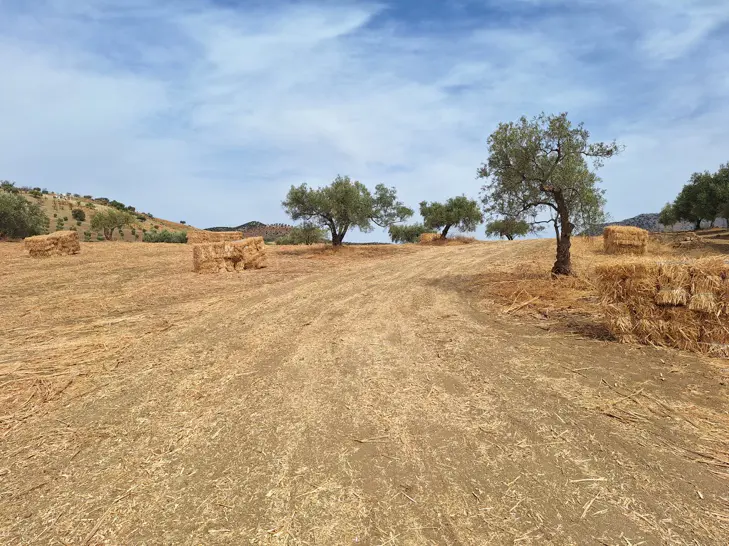
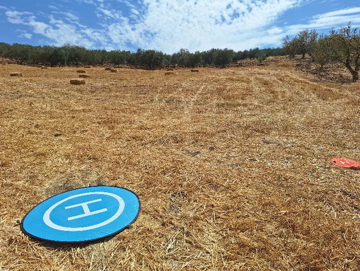
Table 1. UAV characteristics and flight conditions during the experiments.
|
Parameter |
DJI Mavic 2 Enterprise (RGB) |
DJI Mavic 3 Multispectral (M3M) |
Notes/Remarks |
|---|---|---|---|
|
Camera model(s) |
FC2220_4.4_4000 × 3000 (RGB) |
M3M_4.3_2592 × 1944 (Green, Red, Red edge, NIR) + M3M_12.3_5280 × 3956 (RGB) |
Multispectral + RGB rig |
|
Ground Sampling Distance (GSD) |
2.84 cm/pixel |
1.84 cm/pixel |
M3M provides finer spatial resolution |
|
Flight altitude (AGL) |
≈30 m (derived from GSD and focal length) |
≈30 m |
Confirmed the same altitude during mission planning |
|
Image overlap (%) |
Forward 75–80%, Side 70% |
Forward 75–80%, Side 70% |
Consistent grid pattern |
|
Number of images (total/calibrated) |
402 total/378 calibrated (94%) |
2260 total/2260 calibrated (100%) |
M3M captures multi-band datasets |
|
Area covered |
0.170 km2 (≈16.98 ha) |
M3M flight focused on calibration subplot |
|
|
Georeferencing |
GNSS onboard + 6 GCPs (EMLID Reach RS3) |
Higher positional accuracy in M3M data |
|
|
Average keypoints/image |
57,668 |
19,052 |
M2E detects more visual features due to RGB texture richness |
|
Matched keypoints/image |
27,048 |
6303 |
Lower matches in multispectral bands (expected) |
|
3D points generated |
3,116,372 |
1,210,759 |
Dense cloud differences due to the spectral bandwidth |
|
Mean reprojection error |
0.499 px |
0.122 px |
Better geometric accuracy in M3M processing |
|
Relative orientation uncertainty (mean) |
X = 0.225 m; Y = 0.222 m; Z = 0.112 m |
X = 0.008 m; Y = 0.006 m; Z = 0.007 m |
M3M is significantly more stable and precise |
|
DSM/Orthomosaic resolution |
2.84 cm/pixel |
1.84 cm/pixel |
Consistent with flight altitude and sensor specs |
|
Point cloud density |
160.29 pts/m3 |
554.21 pts/m3 |
Denser cloud from M3M multispectral bundle |
|
Coordinate system |
WGS84/UTM Zone 30N (EGM96 Geoid) |
Uniform reference system |
|
|
Illumination sensor |
None |
Integrated sunlight sensor (M3M) |
Allows reflectance calibration |
|
Sampling design |
Full field RGB orthomosaic (entire parcel) |
Subsampled subplot coinciding spatially with RGB frame |
NDVI and RGB data co-registered pixel-to-pixel |
|
Number of valid pixels in analysis |
~38 million (RGB normalized rasters) |
Pixel-wise alignment achieved via rasterio (bilinear resampling) |
|
2.2. Derivation of RGB and NDVI-Based Vegetation Indexes, and Normalization
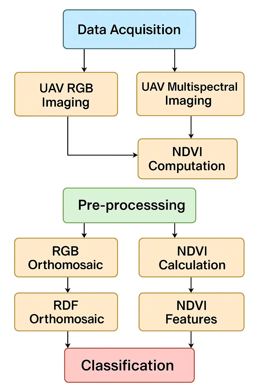
In Figure 2, a flowchart with the entire pipeline in this study is included. From the RGB orthomosaic, four vegetation indexes were derived to evaluate their performance relative to NDVI: the Excess Green index (ExG), the Visible Atmospherically Resistant Index (VARI), the Green Leaf Index (GLI), and the Excess Red index (ExR). All calculations were performed within ArcGIS Pro and implemented through ArcPy scripts to ensure the transparency and reproducibility of the workflow [10,11]. The computation of each index was based on raster algebra applied directly to the red, green, and blue bands of the UAV imagery. ArcPy provided the necessary functionality to automate these operations by combining the Raster object, which allows mathematical operations to be performed directly on raster layers, with conditional functions such as Con for masking NoData values and controlling the output range. Each index was therefore generated as a new raster layer using explicit formulas coded in Python, rather than manual raster calculator operations. This approach allowed the entire process—from loading the orthomosaic bands to exporting the derived indexes—to be scripted, repeated, and adapted to different datasets in a consistent manner. Because each vegetation index is expressed on a different numerical scale, a min–max normalization was applied to all RGB-derived indexes to standardize their values to the range [0, 1]. This ensured that the four indexes could be compared directly, both with each other and with the multispectral NDVI. The NDVI, originally spanning values between −1 and +1, was rescaled to the same range using the transformation:
|
```latex\mathrm{N}\mathrm{D}\mathrm{V}{\mathrm{I}}_{0\text{–}1}=\frac{\mathrm{N}\mathrm{D}\mathrm{V}\mathrm{I}+1}{2}``` |
This normalization step was also automated using ArcPy, which enabled the application of mathematical transformations across all raster cells. To guarantee data integrity, NoData values were handled explicitly: invalid pixels were masked using the SetNull function in ArcPy and later treated as NaN values in Python during the statistical analysis. Finally, a strict clipping was applied to all layers to confine values within the theoretical [0, 1] interval, preventing residual artifacts caused by reprojection or interpolation during preprocessing.
2.3. Co-Registering of Multispectral and RGB Images
To enable a strict pixel-by-pixel comparison between indexes derived from the RGB orthomosaic and the multispectral NDVI, it was necessary to ensure that all datasets shared exactly the same spatial framework. Although both products were georeferenced to the same coordinate system (UTM WGS84 Zone 30N), small differences in resolution or raster grid origin can lead to misalignment. Such discrepancies would result in each pixel representing slightly different ground areas, introducing noise into the statistical comparison. To overcome this issue, the NDVI raster was resampled and aligned to match the grid of the normalized RGB multiband raster. This alignment was carried out in Python using the rasterio library, which allows precise control over raster reprojection and resampling operations. Bilinear resampling was applied, as this method is appropriate for continuous data such as vegetation indexes. It interpolates values from the four nearest pixels, thereby preserving gradients while avoiding the blocky appearance typical of nearest-neighbor resampling.
During this process, the extent, cell size, and coordinate system of the reference raster (the RGB multiband product) were explicitly imposed on the NDVI dataset. This ensured that the two rasters were perfectly coincident, with each pixel in the NDVI map corresponding exactly to the same ground location as the pixels in the RGB-derived indexes. As a result, subsequent comparisons between NDVI and the RGB indexes were performed without geometric distortions or misalignment, guaranteeing that all statistical relationships were computed on a true pixel-to-pixel basis.
2.4. Statistical Analysis
The statistical comparison between NDVI and the RGB-derived indexes was conducted within a Python environment (VS Code) using the libraries rasterio, numpy, pandas, and matplotlib. This combination of tools provided a flexible and reproducible workflow for handling large raster datasets and generating both numerical and graphical outputs. The workflow followed a pixel-level approach, in which values from each RGB index were extracted and paired with their corresponding NDVI values after the alignment process. This pixel-by-pixel pairing ensured that the statistical comparisons were spatially consistent, with each observation representing exactly the same ground location in both datasets. Once extracted, the paired data were used to generate scatterplots, which offered a first visual assessment of the relationships (or lack thereof) between NDVI and the individual RGB indexes.
To quantify these relationships, several descriptive statistics were calculated for each dataset, including the minimum, maximum, mean, and standard deviation, as well as the proportion of pixels with values falling outside the expected [0, 1] interval. These statistics helped to confirm the integrity of the preprocessing steps (normalization and clipping) and evaluate the degree of variability retained in each index. Correlation analyses were performed using the Pearson correlation coefficient (r), providing a measure of the linear association between NDVI and each RGB index [11,12]. To further evaluate agreement, two error metrics were computed: the Root Mean Squared Error (RMSE), which emphasizes larger deviations, and the Mean Absolute Error (MAE), which reflects the average magnitude of differences regardless of direction [13]. Together, these metrics allowed us to assess not only whether RGB indexes followed the same trends as NDVI, but also how closely their values matched in absolute terms.
3. Results
3.1. Vegetation Indexes
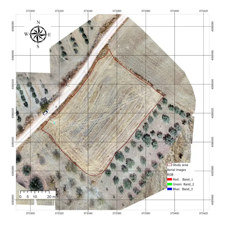
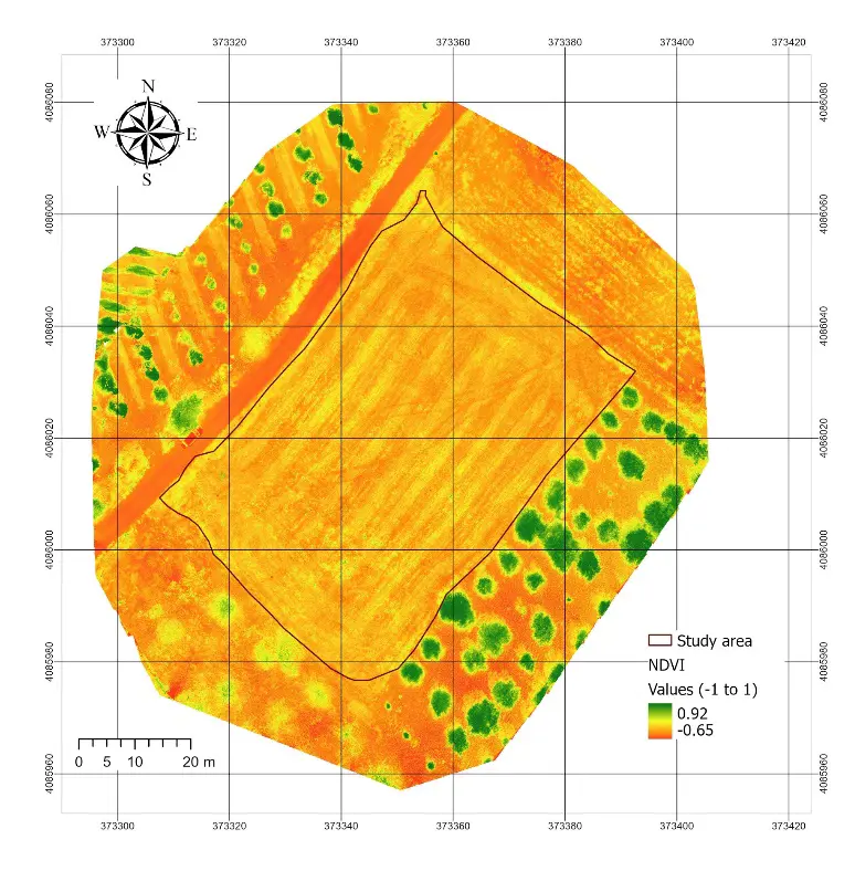
The RGB orthomosaic generated from the DJI Mavic 2 Enterprise provided a high-resolution representation of the study site (Figure 3, left). The field, outlined by the study boundary, clearly displayed the effects of the recent harvest, with most of the surface covered by bare soil and straw residues. Olive trees surrounding the plot were also visible, providing contrasting patches of green vegetation that highlighted the degraded condition of the cereal canopy. The NDVI map derived from the multispectral Mavic 3 imagery (Figure 3, right) showed a restricted range of values within the study area, with most pixels falling between 0.47 and 0.83. Higher NDVI values were concentrated in the olive trees and scattered patches of surviving vegetation, while the harvested cereal field displayed consistently lower NDVI values. This spatial pattern confirmed that, at the time of the survey, the canopy of the cereal field was highly degraded and provided limited photosynthetic activity.
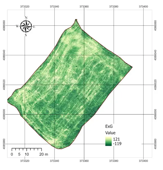
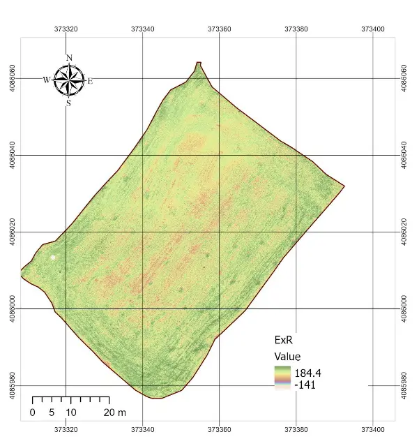
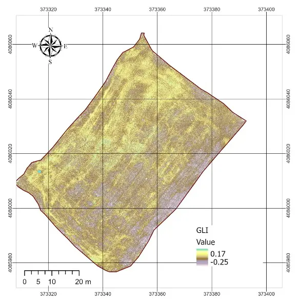
The statistical characterization of the normalized vegetation indexes and the rescaled NDVI is summarized in Table 2. All RGB-based indexes were successfully normalized to the [0–1] interval, with no values falling outside this range. Among the RGB indexes, ExG showed a mean of 0.53 with relatively low variability (standard deviation = 0.022), while ExR displayed the widest spread (standard deviation = 0.038). GLI presented the highest mean value (0.63), whereas VARI was almost constant across the field, with a mean close to 0.495 and a very narrow distribution (standard deviation = 0.0006). By contrast, the rescaled NDVI (NDVI01) had a mean of 0.60 and a wider spread (standard deviation = 0.028), reflecting a more discriminative ability to capture differences in vegetation condition. The spatial patterns observed in the index maps (Figure 4) were consistent with these statistics. ExG and ExR displayed some visible heterogeneity within the field, highlighting linear features associated with harvest machinery tracks and subtle contrasts between soil and residues. GLI produced intermediate values across the entire plot, but the contrast between areas was relatively muted. In contrast, VARI produced a nearly uniform map, confirming the statistical observation of its lack of variability and explaining its limited usefulness under post-harvest conditions. Overall, the NDVI map retained the clearest spatial variability, while the RGB-based indexes, despite being sensitive to some structural features, exhibited compressed distributions and reduced dynamic range.
 |
 |
 |
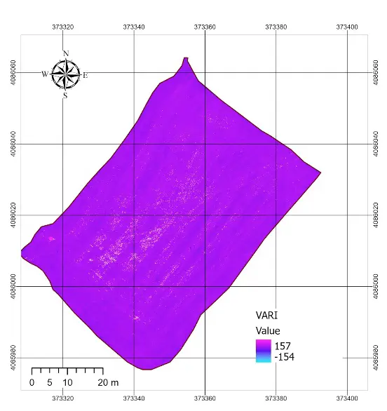 |
Figure 4. RGB indexes applied in the study area. ExG = Excess Green, VARI = Visible Atmospherically Resistant Index, GLI = Green Leaf Index, ExR = Excess Red.
Table 2. Descriptive statistics of normalized RGB vegetation indexes and rescaled NDVI (0–1) for the study area.
|
Index |
n |
Min |
Max |
Mean |
Std. Dev. |
|---|---|---|---|---|---|
|
ExG |
38,251,063 |
0.000 |
1.0 |
0.526 |
0.022 |
|
VARI |
38,251,063 |
0.000 |
1.0 |
0.495 |
0.001 |
|
GLI |
38,251,063 |
0.000 |
1.0 |
0.625 |
0.022 |
|
ExR |
38,251,063 |
0.000 |
1.0 |
0.659 |
0.038 |
|
NDVI01 |
38,251,063 |
0.470 |
0.84 |
0.600 |
0.028 |
ExG = Excess Green, VARI = Visible Atmospherically Resistant Index, GLI = Green Leaf Index, ExR = Excess Red, NDVI01 = NDVI rescaled from −1 to +1 into 0–1. n = number of valid pixels included in the analysis; Min and Max represent the minimum and maximum values observed in each raster; Mean = arithmetic mean; Std. Dev. = standard deviation, as a measure of variability.
3.2. Distribution of Indexes: Histogram Analysis
The comparative histograms of the normalized RGB indexes and the rescaled NDVI (Figure 5) provided additional insight into their behavior. The NDVI01 values were distributed between ~0.47 and 0.83, with a clear peak around 0.60, reflecting moderate heterogeneity within the field. By contrast, ExG and ExR displayed narrower distributions centered around 0.52–0.66, indicating a reduced ability to capture variability in canopy conditions. GLI showed a slightly wider distribution but remained concentrated between 0.60 and 0.65, confirming its compressed range observed in the descriptive statistics. The most striking result was VARI, which collapsed into an almost uniform distribution around 0.495, producing a sharp peak and effectively behaving as a constant variable across the study area.
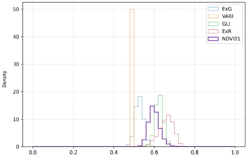
Figure 5. Histogram including a comparison of RGB and NDVI-based vegetation indexes. ExG = Excess Green, VARI = Visible Atmospherically Resistant Index, GLI = Green Leaf Index, ExR = Excess Red, NDVI01 = NDVI rescaled from −1 to +1 into 0–1.
3.3. RGB vs. NDVI
The statistical comparison revealed that RGB indexes showed very weak correlations with NDVI under post-harvest conditions (Table 3). ExR achieved the highest correlation coefficient (r = 0.128), followed by ExG (r = 0.090), while GLI displayed almost no association (r = 0.016). VARI showed a slightly negative correlation (r = −0.039), confirming its lack of sensitivity in this scenario. The error metrics also highlighted the discrepancies: RMSE values for ExG and ExR exceeded 0.14, whereas GLI and VARI produced lower RMSE values but without meaningful correlation. These results demonstrate that none of the RGB indexes were able to reliably reproduce NDVI variability when the canopy was degraded and dominated by soil and straw residues.
Table 3. Correlation and error metrics between RGB vegetation indexes and NDVI (0–1).
|
Pair |
Pearson r |
RMSE |
MAE |
n |
|---|---|---|---|---|
|
ExG vs. NDVI |
0.090 |
0.145 |
0.109 |
79,158,779 |
|
VARI vs. NDVI |
−0.039 |
0.109 |
0.105 |
38,251,063 |
|
GLI vs. NDVI |
0.016 |
0.043 |
0.035 |
38,251,073 |
|
ExR vs. NDVI |
0.128 |
0.165 |
0.131 |
79,158,779 |
Pearson r indicates the strength of the linear correlation between NDVI and each RGB index; RMSE = Root Mean Squared Error; MAE = Mean Absolute Error; n = number of valid paired pixels included in the comparison.
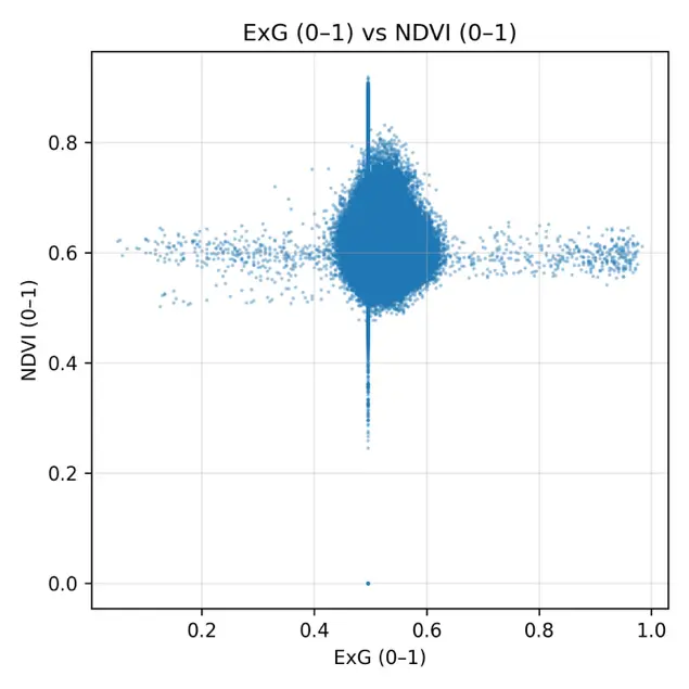
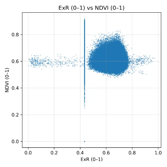
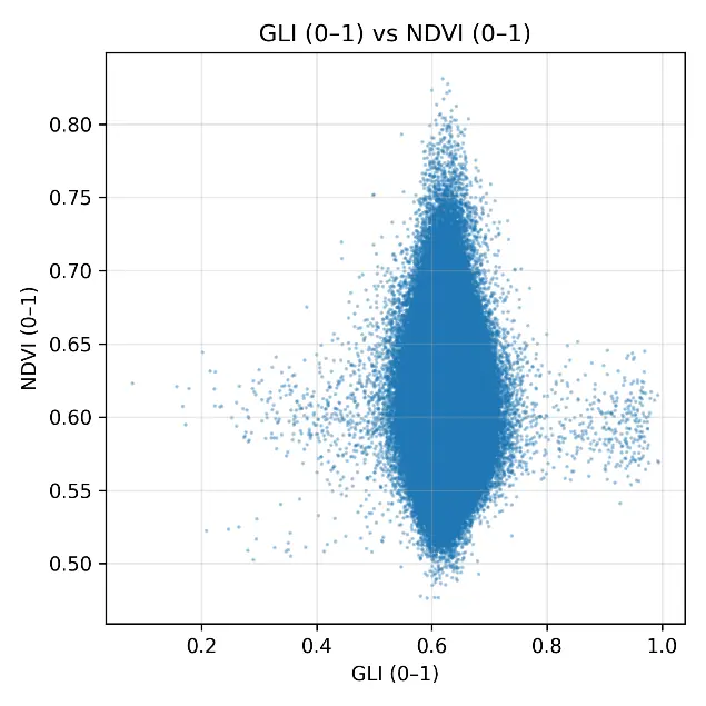
The scatterplots comparing NDVI with each RGB-based index (Figure 6) provided a detailed visualization of the weak statistical associations observed in Table 3. The ExG scatterplot showed a dense clustering of points around NDVI values of 0.55–0.65 and ExG values of 0.45–0.60, with no clear linear trend, confirming the low correlation (r = 0.090). ExR displayed a slightly wider spread, with some variability across the field, but still lacked a consistent linear relationship with NDVI, consistent with its moderate error values. GLI produced a compact distribution of points aligned vertically around 0.60, illustrating its compressed range and inability to capture differences in NDVI despite its low RMSE. The most extreme case was VARI, which collapsed almost entirely into a vertical line at ~0.50, confirming the near-constant behavior already noted in the histograms and descriptive statistics. Overall, the scatterplots reinforced the finding that RGB indexes could not reproduce the variability of NDVI under post-harvest conditions. Even though ExR and ExG retained some heterogeneity, their relationships with NDVI were too weak to be meaningful, whereas GLI and, especially, VARI offered almost no discriminative capacity. These results illustrate the limitations of RGB-based monitoring when canopy cover is minimal and spectral signals are dominated by soil and dry residues.
 |
 |
 |
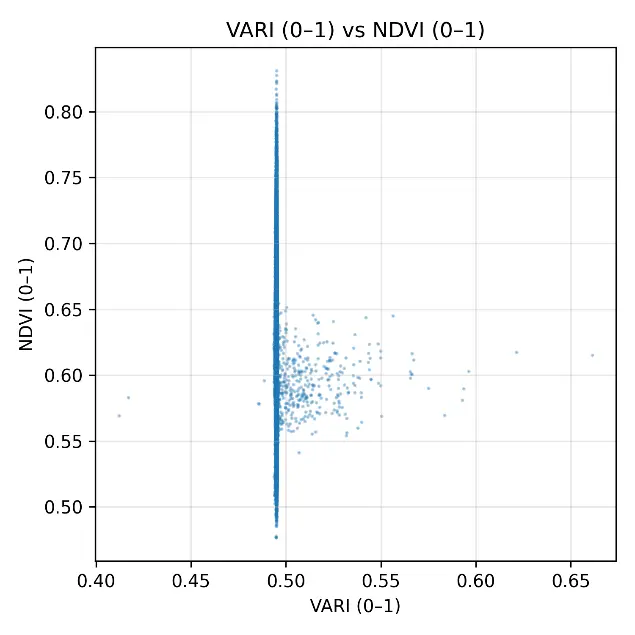 |
Figure 6. Scatterplots comparing normalized RGB vegetation indexes (ExG, ExR, GLI, VARI) with rescaled NDVI (0–1) under post-harvest conditions in the cereal field. Each panel shows the pixel-by-pixel relationship between indexes, with values standardized to the range [0–1].
4. Discussion
The results of this study demonstrate the strong influence of canopy condition on the performance of RGB-based vegetation indexes when compared with NDVI. Under post-harvest conditions, when most of the green biomass was removed and the surface was dominated by bare soil and crop residues, all RGB indexes displayed very weak correlations with NDVI (Pearson r < 0.15). This outcome contrasts with previous reports showing significant correlations between RGB indexes and NDVI during the active growing stages of cereals, highlighting that the reliability of RGB indexes is strongly stage-dependent [14,15]. One of the key findings is that certain indexes, such as VARI, collapsed into almost constant values across the field, showing minimal variability. This behavior can be explained by the fact that VARI was designed to minimize atmospheric effects and enhance green vegetation in conditions of relatively high canopy cover [16,17]. When green vegetation is largely absent, as in our post-harvest field, the spectral contribution of soil and dry residues dominates the signal, effectively flattening the index. In contrast, indexes such as GLI and ExR retained a slightly broader distribution, although still failing to capture the full variability expressed by NDVI. These patterns confirm that indexes relying solely on visible bands cannot substitute the near-infrared response, which is fundamental to detecting differences in canopy vigor. The histograms further reinforced these observations. While NDVI values covered a broader range (0.47–0.83), reflecting subtle differences in the amount of green vegetation remaining after harvest, the RGB-based indexes showed compressed distributions, with low standard deviations and limited spread around central values. This compression reduces their discriminative capacity and explains the weak correlations observed in the scatterplots. Importantly, the methodological steps of normalization and clipping ensured that this limitation was not caused by preprocessing artifacts but reflected the intrinsic properties of the indexes under degraded canopy conditions.
From a methodological perspective, these findings carry important implications for UAV-based crop monitoring. RGB imagery offers clear advantages in terms of cost, accessibility, and ease of deployment [18], and RGB indexes can indeed serve as practical proxies for vegetation status during active crop growth [15]. However, their use becomes highly unreliable when canopy cover decreases sharply, such as after harvest or under severe abiotic stress. In such cases, multispectral imagery that includes the near-infrared band remains essential for accurate assessment [19,20]. Thus, while RGB indexes are suitable for preliminary monitoring, they should not be relied upon in phases where vegetation is sparse or deteriorated. Finally, in the context of abiotic stress research in cereals, our results highlight the importance of carefully considering the phenological stage of the crop when selecting UAV sensors and indexes. Post-harvest or degraded canopy conditions represent an extreme scenario where RGB indexes are not informative, and their direct comparison with NDVI may lead to misleading interpretations. This methodological note therefore emphasizes the need for caution when applying RGB-derived indexes beyond optimal growth stages and provides evidence-based guidance for future UAV studies on cereal stress monitoring.
Soil background and illumination effects were also considered when interpreting the spectral discrepancies between UAV products. The cereals were partially interspersed with exposed soil, whose reflectance strongly influences RGB-derived vegetation indices through the so-called “soil line” effect, especially in the visible bands [21,22]. Under variable illumination, non-vegetated pixels can increase index variability and reduce the apparent contrast between canopy and background, particularly for indices that do not normalize brightness (e.g., ExG). By contrast, normalized indices such as VARI and NGRDI tend to minimize these effects by expressing the relative contribution of the green channel to the total visible reflectance. Although no explicit spectral calibration was performed, both UAVs were flown under stable midday conditions to reduce directional illumination effects. The residual differences observed are thus mainly attributable to radiometric response and sensor optics rather than soil background. Future applications could benefit from integrating soil-masking techniques or linear soil-line corrections to further harmonize cross-platform RGB indices.
5. Conclusions
This study assessed the relationship between UAV-derived RGB vegetation indexes and NDVI under post-harvest conditions in a cereal field. Using a combination of ArcGIS Pro, ArcPy, and Python libraries, we generated and normalized four indexes (ExG, ExR, VARI, and GLI), aligned them with multispectral NDVI, and carried out pixel-by-pixel statistical comparisons. The results consistently showed very weak correlations between RGB indexes and NDVI (r < 0.15), with compressed distributions and limited variability in the RGB indexes compared to the broader range of NDVI. These findings highlight a fundamental methodological limitation: RGB indexes, while useful during active crop growth, lose reliability when canopy cover is reduced due to harvest or degradation. The absence of near-infrared reflectance in RGB imagery prevents these indexes from capturing subtle differences in vegetation vigor once green biomass is scarce. As a result, their application to post-harvest or severely stressed cereal fields may lead to misleading conclusions. In practical terms, the study demonstrates that RGB-based UAV monitoring can complement multispectral approaches during the growing season but should not be considered a substitute under degraded canopy conditions. For research focused on abiotic stress in cereals, these results provide clear evidence that sensor and index selection must take crop phenology into account. Therefore, this work serves as a methodological note, underscoring both the potential and the limitations of RGB indexes in agricultural remote sensing.
Statement of the Use of Generative AI and AI-Assisted Technologies in the Writing Process
During the preparation of this manuscript, the authors used Chat GPT to review grammar and typos. After using this tool/service, the authors reviewed and edited the content as needed and take(s) full responsibility for the content of the published article.
Author Contributions
Conceptualization, J.R.-C., V.H.D.-Z., F.S.-B., A.C.-C. and V.R.-G.; Methodology, J.R.-C. and V.R.-G.; Validation, J.R.-C., V.H.D.-Z., F.S.-B., A.C.-C. and V.R.-G.; Formal Analysis, J.R.-C., A.A.G.A.-S. and V.R.-G.; Investigation, J.R.-C., A.A.G.A.-S., V.H.D.-Z., F.S.-B., A.C.-C. and V.R.-G.; Data Curation, J.R.-C., Writing—Original Draft Preparation, J.R.-C., V.H.D.-Z., F.S.-B., A.C.-C. and V.R.-G.; Writing—Review & Editing, J.R.-C., V.H.D.-Z., F.S.-B., A.C.-C. and V.R.-G.; Project Administration, J.R.-C., and V.R.-G.; Funding Acquisition, J.R.-C. and V.R.-G.
Ethics Statement
Not applicable.
Informed Consent Statement
Not applicable.
Data Availability Statement
The data can be shared upon due request.
Funding
This research was funded by the project “Desarrollo de productos basados en los nuevos sensores satelitales hiperespectrales europeos e IA para la caracterización de estresores en tierras de cultivo (HIPROESTRES)” (grant number PID2023-152656OB-I00), within the Programa Estatal de Investigación Científica, Técnica y de Innovación (2021-2023) by the Ministerio de Ciencia, Innovación y Universidades.
Declaration of Competing Interest
The authors declare that they have no known competing financial interests or personal relationships that could have appeared to influence the work reported in this paper.
References
-
Weiss M, Jacob F, Duveiller G. Remote Sensing for Agricultural Applications: A Meta-Review. Remote Sens. Environ. 2020, 236, 111402. doi:10.1016/j.rse.2019.111402. [Google Scholar]
-
Sishodia RP, Ray RL, Singh SK. Applications of Remote Sensing in Precision Agriculture: A Review. Remote Sens. 2020, 12, 3136. doi:10.3390/rs12193136. [Google Scholar]
-
Umirzakova S, Muksimova S, Shavkatovich Buriboev A, Primova H, Choi AJ. A Unified Transformer Model for Simultaneous Cotton Boll Detection, Pest Damage Segmentation, and Phenological Stage Classification from UAV Imagery. Drones 2025, 9, 555. doi:10.3390/drones9080555. [Google Scholar]
-
Huang S, Tang L, Hupy JP, Wang Y, Shao G. A Commentary Review on the Use of Normalized Difference Vegetation Index (NDVI) in the Era of Popular Remote Sensing. J. For. Res. 2021, 32, 1–6. doi:10.1007/s11676-020-01155-1. [Google Scholar]
-
Cao X, Liu Y, Yu R, Han D, Su B. A Comparison of UAV RGB and Multispectral Imaging in Phenotyping for Stay Green of Wheat Population. Remote Sens. 2021, 13, 5173. doi:10.3390/rs13245173. [Google Scholar]
-
García-Fernández M, Sanz-Ablanedo E, Rodríguez-Pérez JR. High-Resolution Drone-Acquired RGB Imagery to Estimate Spatial Grape Quality Variability. Agronomy 2021, 11, 655. doi:10.3390/agronomy11040655. [Google Scholar]
-
Doornbos J, Babur Ö, Valente J. Evaluating Generalization of Methods for Artificially Generating NDVI from UAV RGB Imagery in Vineyards. Remote Sens. 2025, 17, 512. doi:10.3390/rs17030512. [Google Scholar]
-
Colovic M, Stellacci AM, Mzid N, Di Venosa M, Todorovic M, Cantore V, et al. Comparative Performance of Aerial RGB vs. Ground Hyperspectral Indices for Evaluating Water and Nitrogen Status in Sweet Maize. Agronomy 2024, 14, 562. doi:10.3390/agronomy14030562. [Google Scholar]
-
Feng H, Tao H, Li Z, Yang G, Zhao C. Comparison of UAV RGB Imagery and Hyperspectral Remote-Sensing Data for Monitoring Winter Wheat Growth. Remote Sens. 2022, 14, 3811. doi:10.3390/rs14153811. [Google Scholar]
-
Tulu BB, Teshome F, Ampatzidis Y, Hailegnaw NS, Bayabil HK. AgriSenAI: Automating UAV Thermal and Multispectral Image Processing for Precision Agriculture. SoftwareX 2025, 30, 102083. doi:10.1016/j.softx.2025.102083. [Google Scholar]
-
Ullah S, Ilniyaz O, Eziz A, Ullah S, Fidelis GD, Kiran M, et al. Multi-Temporal and Multi-Resolution RGB UAV Surveys for Cost-Efficient Tree Species Mapping in an Afforestation Project. Remote Sens. 2025, 17, 949. doi:10.3390/rs17060949. [Google Scholar]
-
Duan B, Fang S, Zhu R, Wu X, Wang S, Gong Y, et al. Remote Estimation of Rice Yield With Unmanned Aerial Vehicle (UAV) Data and Spectral Mixture Analysis. Front. Plant Sci. 2019, 10, 204. doi:10.3389/fpls.2019.00204. [Google Scholar]
-
Hodson TO. Root-Mean-Square Error (RMSE) or Mean Absolute Error (MAE): When to Use Them or Not. Geosci. Model Dev. 2022, 15, 5481–5487. doi:10.5194/gmd-15-5481-2022. [Google Scholar]
-
Wang L, Duan Y, Zhang L, Rehman TU, Ma D, Jin J. Precise Estimation of NDVI with a Simple NIR Sensitive RGB Camera and Machine Learning Methods for Corn Plants. Sensors 2020, 20, 3208. doi:10.3390/s20113208. [Google Scholar]
-
Davidson C, Jaganathan V, Sivakumar AN, Czarnecki JMP, Chowdhary G. NDVI/NDRE Prediction from Standard RGB Aerial Imagery Using Deep Learning. Comput. Electron. Agric. 2022, 203, 107396. doi:10.1016/j.compag.2022.107396. [Google Scholar]
-
Gerardo R, de Lima IP. Applying RGB-Based Vegetation Indices Obtained from UAS Imagery for Monitoring the Rice Crop at the Field Scale: A Case Study in Portugal. Agriculture 2023, 13, 1916. doi:10.3390/agriculture13101916. [Google Scholar]
-
Hasan U, Sawut M, Chen S. Estimating the Leaf Area Index of Winter Wheat Based on Unmanned Aerial Vehicle RGB-Image Parameters. Sustainability 2019, 11, 6829. doi:10.3390/su11236829. [Google Scholar]
-
González-Moreno MT, Rodrigo-Comino J. Geostatistical Vegetation Filtering for Rapid UAV-RGB Mapping of Sudden Geomorphological Events in the Mediterranean Areas. Drones 2025, 9, 441. doi:10.3390/drones9060441. [Google Scholar]
-
Aldakheel YY. Assessing NDVI Spatial Pattern as Related to Irrigation and Soil Salinity Management in Al-Hassa Oasis, Saudi Arabia. J. Indian Soc. Remote Sens. 2011, 39, 171–180. [Google Scholar]
-
Ding Y, Zhao K, Zheng X, Jiang T. Temporal Dynamics of Spatial Heterogeneity over Cropland Quantified by Time-Series NDVI, near Infrared and Red Reflectance of Landsat 8 OLI Imagery. Int. J. Appl. Earth Obs. Geoinf. 2014, 30, 139–145. doi:10.1016/j.jag.2014.01.009. [Google Scholar]
-
Baret F, Guyot G. Potentials and Limits of Vegetation Indices for LAI and APAR Assessment. Remote Sens. Environ. 1991, 35, 161–173. doi:10.1016/0034-4257(91)90009-U. [Google Scholar]
-
Huete AR, Jackson RD, Post DF. Spectral Response of a Plant Canopy with Different Soil Backgrounds. Remote Sens. Environ. 1985, 17, 37–53. doi:10.1016/0034-4257(85)90111-7. [Google Scholar]