1. Introduction
India is ranked sixth in the Climate Risk Index (CRI) 2025 according to a report [
1], highlighting its vulnerability to extreme weather events and their impacts. While India has improved its short-term CRI rank, it remains among the top 10 countries most affected by extreme weather events historically, between 1993 and 2022, according to the same report. The report shows that India faced over 400 extreme weather events, resulting in approximately 80,000 fatalities and nearly $180 billion in economic losses between 1993 and 2022. In vast stretches of the developing regions of the world, the number of people and places that will experience extreme climate variability events, e.g., drought, is expected to rise rapidly in this century due to the effects of climate change [
2]. Growing incidences of climate variability events such as drought combined with sensitive socioeconomic characteristics in rural India; such as; high poverty level, high borrowing level, high illiteracy rate, high dependency ratio, less crop diversity, agriculture as the only source of income, low level of agricultural insurance
etc. make people more vulnerable [
3,
4,
5]. Drought brings multiple pressures across the rural economy, society and environment [
2,
6,
7], and drought-affected rural areas may experience large-scale out-migration of population [
8,
9,
10].
Migration is a process that affects the areas undergoing in-migration, as well as areas of out-migration, along with the migrants themselves. In the development literature, a debate has been ongoing for several decades between migration prevention and migration support policy approaches [
11,
12]. The early scholarly literature on climate change-induced migration primarily described migration as a failure of adaptation to climate change [
13]. Since roughly 2010, around the publication of Foresight report [
14], a new hypothesis that gained momentum in the writings of many researchers is whether migration can be considered as one of a form of adaptation strategies in the face of climate change [
15,
16,
17,
18,
19,
20,
21,
22,
23]. This hypothesis provided direction for the scholarly literature development in the field (if it can be described as such) of environmental migration during the decade that followed, including the present time.
Migration may be considered as adaptation if the households affected by migration can live equally well or better after the migration [
24]. Migration may not be described as adaptation in situations in which migrants face poverty traps or experience cultural loss. The effect of migration on adaptive capacities may be studied at three points: the origin population, the destination population and the migrants themselves [
25]. Migration may affect adaptation capabilities at origin and destination communities through shaping opportunities for (1) remittances and capital inflow; (2) skills and knowledge; (3) livelihood diversification and social capital of migrant networks; (4) institutions, cooperation and co-development [
26]. Migration may also serve as an adaptation strategy as it reduces population pressure on limited resources, facilitates risk reduction, and thus offers those who stay behind better chances for survival [
25].
Several limitations of the hypothesis were also voiced time to time: migration may become an important adaptation response after environmental degradation has reached a certain threshold [
16]; migration may be an adaptation strategy after households have exhausted all other in-situ adaptation strategies at the face of adverse environmental conditions [
27]; the fewer choices people have about migrating, the less likely the outcomes of that migration will be positive [
17]; the trend to migrate to cities also involves risk for migrant populations [
28]; the notion requires consideration of multiple types and dimensions of vulnerability as what constitutes adaptation for some may become maladaptation in other parts of the system [
21]; migration should not be advocated over non-migration just to hide governance failures that led to human suffering and migration [
24]. Migration as an adaptation hypothesis should not neglect the adaptive capacities of non-migrants and the overall community at origin [
25].
Such a shift in the conceptualization of migration may also have its bearing on the formulation of migration policies. Coordinated policies are required that may recognize how and why people move [
29]; may expand opportunities for migration [
15]; may understand of the role of local and national institutions in supporting and accommodating migration [
30]; may ensure that the socioeconomic and humanitarian outcomes are maximized [
16]; may minimize the risks associated with migration and maximize migration’s contribution to adaptive capacity building [
17].
Many studies have emerged in the last one and a half decade which examine the effects of migration on building adaptive capacity to climate change or climate variability in general, focusing on developing countries. A few empirical studies have tried to investigate the contribution of migration on peoples’ adaptation to drought in Canada [
27], West African Sahel [
22], Ethiopia [
31], Kenya [
32], Syria [
33]
etc. and reported a wide range of experiences that migrants faced at both source and destination areas. In India, there may be hardly any study which specifically measures the impacts of migration on drought adaptation but there exist a few case studies on how migration may impact on adaptation to climate variability (such as 34–37). The results of these case studies broadly indicate a mixed pattern of impacts that migration may have on climate variability adaptation, making it difficult to draw any straightforward conclusions from the “migration as adaptation” hypothesis.
With this background, the present study tried to assess the impacts of temporary migration on the adaptive capacity of households in the face of climate variability (e.g., drought) in rural India with IHDS 2nd round (2011–12) and IMD rainfall binary files fitted into propensity score matching methods. The rest of the paper will provide a description of the materials used, results of the analyses, a discussion on the results and finally a conclusion. A description of the method applied,
i.e., propensity score matching, is provided in Appendix A.
2. Materials and Methods
2.1. Socioeconomic Data
The study was based on socioeconomic data generated through the second round of the nationally representative and multi-topic India Human Development Survey (IHDS), conducted in 2011–12 (hereinafter referred to as IHDS-II). The data were jointly generated by the National Council of Applied Economic Research (NCAER), New Delhi and the University of Maryland, with funding provided by the National Institutes of Health (NIH). Geographically, the survey covered all states and union territories in India except for the Andaman and Nicobar Islands and the Lakshadweep Islands using stratified random sampling methods. IHDS-II surveyed 42,152 households (27,579 rural and 14,573 urban) and 204,569 individuals (135,118 rural, 69,450 urban and 1 uncategorized) in 1420 villages and 1042 urban neighbourhoods spread across 384 districts in India. Two one-hour interviews were conducted in each household to collect information on income, social capital, education, and health. The data were publicly available on the Inter-University Consortium for Political and Social Research (ICPSR) website Available at https://www.icpsr.umich.edu/web/DSDR/studies/36151/datadocumentation (accessed on 15 March 2023), which contained more information regarding data collection and data structure.
2.2. Sample Size
IHDS-II consisted of 42,152 households, as described above. After subtracting 14,573 urban households (urban residence as per Census 2011), the sample size was reduced to 27,579 households (65.4%). Five households had no data related to household heads, which reduced the sample size to 27,574 households. After removing the households with missing data (1 religion, 28 social group, 8 occupations, 14 household expenditure, 5 education, 35 land, 493 income, 3393 income from agriculture and 11 income from business), the final sample size for the study stood at 23,586 households. This aggregate sample size was divided into five equal monthly per capita expenditure (MPCE) quintiles, with each around 4717 observations. The same aggregate sample was again divided into four social groups; Others (
n = 6222), Other Backward Classes (
n = 9481), Scheduled Castes (
n = 5200) and Scheduled Tribes (
n = 2683).
2.3. Outcome Variables
The study focused on the impact of temporary migration on building household adaptive capacity to climate variability (e.g., drought). Intergovernmental Panel on Climate Change (IPCC) working group II in its sixth assessment report defined adaptation as:
“Adaptation is defined, in human systems, as the process of adjustment to actual or expected climate and its effects in order to moderate harm or take advantage of beneficial opportunities.” [
34].
The idea of the contribution of migration in building adaptive capacity might be operationalized through two popular theoretical approaches in migration literature; one, migration helped the households in improving their economic well-being through utility maximization as argued in the neoclassical migration theory [
35]; two, migration might act as a risk-diversification strategy where the household members got involved into multiple sectors where the earnings were statistically uncorrelated to each other as put forward by the new economics of labour migration [
36].
Monthly per capita consumption expenditure (MPCE) might be an important indicator for the success of migration in the case of the utility maximization approach, whereas livelihood diversity (LD) and share of non-agricultural income (INCNAG) might be important indicators for the risk-diversification approach. It might be argued that these variables not only cater to the adaptive capacity in the face of climate variability but also other shocks and stresses through risk pooling, risk distribution or as a buffer during extreme climatic events [
37,
38]. Households with higher MPCE might be associated with higher adaptive capacity in the face of climate variability, as they may have greater expenditure capacity left over after meeting basic expenses for food and shelter. Higher MPCE meant more resources were available at disposal for the maximization of positive livelihood outcomes. This financial capacity may serve as an effective buffer against the effects of climate variability.
A diversified livelihood portfolio comprising various livelihood strategies with differing susceptibilities to climate variability may help increase the adaptive capacity of households in the face of climate variability. As if one livelihood strategy faced pressure from climate variability, the income from other livelihood strategies might help the household survive the stress. The proportion of income from non-agricultural sources might indicate the degree to which a household was free from the direct susceptibility of environmental variables for making a living.
describes the measurement and description of the three indicators.
.
Description of outcome variables.
| Variable |
Measurement |
Description |
| MPCE |
Values in Rupees |
Monthly per capita consumption expenditure of the household |
| LD |
Index value ranging from 1 to 6 |
Livelihood diversity index at household level was calculated using the inverse Herfindahl-Hirschman Diversity Index (HHDI) following Anderson and Deshingkar [39]: |
| $$H H D I_{i} = \left(\frac{1}{\sum a \frac{2}{j}}\right)_{i}$$ |
(1) |
| where aj represents the proportional contribution of each livelihood activity j to household i’s overall annual income. In the study, six livelihood activities or income sources were considered: agriculture; business; income from property, pensions, etc.; wage and salary earnings with bonuses; all government benefits; and remittances. Households with zero or negative income were excluded from the analysis. Across the six sources of income, negative contributions were excluded. |
| INCNAG |
% |
Proportion of non-agricultural income in the total annual income. In the study, non-agricultural income sources consist of business; income from property, pensions etc.; wage and salary earnings with bonuses; all government benefits; and remittances. |
2.4. Treatment Variable
Temporary migration was the treatment variable in the analysis. A temporary migrant was any member of the household who left to find seasonal/ short-term work during the last one year and returned back to their origin. If the household had at least one temporary migrant member, then the household was considered to have received the treatment and coded as 1, otherwise, it was considered that the household had undergone no treatment and coded as 0. Out of the 23,586 households, which constituted the aggregate sample size for this study, 4.9% (1162) of the households had at least one temporary migrant member. The share of the households with at least one temporary migrant member across the five MPCE quintiles were: 30.9% (359) in quintile 1, 25.6% (297) in quintile 2, 19.6% (228) in quintile 3, 14.5% (169) in quintile 4, and 9.4% (109) in quintile 5. The share of households with at least one temporary migrant member across the four social groups was 13.4% (156) in Others, 42.3% (491) in Other Backward Classes, 26.2% (304) in Scheduled Castes and 18.2% (211) in Scheduled Tribes. At the weighted individual level, 98.9% of migrants moved internally, and 59.2% of migrants were rural to urban migrants.
2.5. Covariates
A set of variables was considered that could impact the treatment status and/or the outcome under study. These covariates were compiled from both IHDS-II and India Meteorological Department (IMD) gridded binary rainfall files. The covariates considered in this study were one meteorological variable of drought; seven household level variables, e.g., household size, household with long-term migrant(s), religion, social group, land possession, occupation type, and income per capita; four variables describing the demographic characteristics of the household head, e.g., sex, age, marital status, and educational level and one geographical variable in terms of state as described in
.
.
Description of covariates.
| Variable |
Measurement |
Description |
| Meteorological variable |
| Drought |
1 = no,
2 = yes
|
If a district registered the total annual rainfall for a year well below (by at least an amount of 40% or more) than the normal annual rainfall (it’s a 50 years average of annual rainfalls between 1951 and 2000 for that district) for at least one year between 2007 and 2011 (i.e., within last five years before IHDS-II took place), that district was recorded as drought-affected. IMD gridded binary rainfall files a were processed with GRADS 2.2 and R 3.6.3 to generate the data on drought at the district level, which were later on merged with IHDS-II data. |
| Household level variable |
| Household size |
Number |
Number of members in a household. |
| Household with long-term migrant(s) |
1 = yes,
2 = no
|
This information was captured under the theme “Non-Resident Family Members”. |
| Religion |
1 = Hinduism,
2 = Islam,
3 = Others
|
Religion of the household head. |
| Social group |
1 = Others,
2 = OBC,
3 = SC,
4 = ST
|
Social group the household belongs to. |
| Land possession |
Area in acre |
Agricultural land owned by the household. |
| Occupation type |
1 = self-employed in agriculture,
2 = self-employed in non-agriculture,
3 = agricultural labour,
4 = other labour,
5 = others
|
Principal source of income for the household. |
| Income per capita |
Values in Rupees |
Annual per capita income of the household. Income has six components: agriculture; business; income from property, pensions etc.; wage and salary earnings with bonuses; all government benefits; and remittances. |
| Household head characteristic |
| HHH Sex |
1 = male,
2 = female
|
Sex of the household head. |
| HHH Age |
Number |
Age of the household head. |
| HHH Marital status |
1 = currently married,
2 = never married,
3 = widowed,
4 = divorced/separated
|
Marital status of the household head. |
| HHH Educational level |
1 = not literate,
2 = literate but up to primary,
3 = above primary but up to secondary,
4 = above secondary
|
Standard years of education completed by the household head. |
| Geographical variable |
| State |
1 = Jammu and Kashmir,
2 = Himachal Pradesh,
3 = Punjab,
5 = Uttarakhand,
6 = Haryana,
7 = Delhi,
8 = Rajasthan,
9 = Uttar Pradesh,
10 = Bihar,
11 = Sikkim,
12 = Arunachal Pradesh,
13 = Nagaland,
14 = Manipur,
15 = Mizoram,
16 = Tripura,
17 = Meghalaya,
18 = Assam,
19 = West Bengal,
20 = Jharkhand,
21 = Odisha,
22 = Chhattisgarh,
23 = Madhya Pradesh,
24 = Gujarat,
25 = Daman and Diu,
26 = Dadra and Nagar Haveli,
27 = Maharashtra,
28 = Andhra Pradesh,
29 = Karnataka,
30 = Goa,
32 = Kerala,
33 = Tamil Nadu,
34 = Pondicherry
|
State of residence of the household during survey. |
3. Results
3.1. Effects of Temporary Migration on Household Adaptive Capacity in Aggregate Sample
According to the PSM results at aggregate level as described in
, households with at least one temporary migrant member had less monthly per capita consumption expenditure (MPCE) compared to households without any temporary migrant member (treated mean MPCE Rs. 1390.539, control mean MPCE Rs. 1408.563), but the difference was statistically not significant against an one-sided alternative. In terms of livelihood diversity (LD), households with at least one temporary migrant member scored better than households without any temporary migrant member (treated mean LD index 1.518, control mean LD index 1.497) at 10% level of significance. In terms of share of non-agricultural income (INCNAG), households with at least one temporary migrant member performed better than households without any temporary migrant member (treated mean INCNAG 73.529%, control mean INCNAG 70.602%) at 1% level of significance. As per the unmatched estimates, though the directions of differences between the treated and control means remained the same as with the matched estimates, but their magnitudes were significantly higher before matching.
.
Propensity score matching results for aggregate sample (Radius matching with caliper 0.01).
| Variable |
Sample |
Treated |
Controls |
Difference |
S.E. |
T-Stat |
p > |t| |
| MPCE |
Unmatched |
1390.539 |
1916.975 |
−526.436 |
64.478 |
−8.16 |
*** |
| ATT |
1390.539 |
1408.563 |
−18.024 |
40.840 |
−0.44 |
|
| LD |
Unmatched |
1.518 |
1.483 |
0.035 |
0.015 |
2.27 |
** |
| ATT |
1.518 |
1.497 |
0.022 |
0.016 |
1.33 |
* |
| INCNAG |
Unmatched |
73.529 |
69.130 |
4.399 |
1.055 |
4.17 |
*** |
| ATT |
73.529 |
70.602 |
2.927 |
0.968 |
3.02 |
*** |
3.2. Effects of Temporary Migration on Household Adaptive Capacity: Disaggregated Analysis across MPCE Quintiles, Social Groups, and Districts with and without Droughts
A disaggregated analysis across the different expenditure quintiles found that the improved benefits of temporary migration (especially in terms of the share of non-agricultural income) were largely concentrated in the middle and higher expenditure classes (
).
.
Propensity score matching results across MPCE quintiles (Radius matching with caliper 0.01).
| Variable |
Sample |
Treated |
Controls |
Difference |
S.E. |
T-Stat |
p > |t| |
| MPCE quintile 1 |
| MPCE |
ATT |
643.749 |
651.924 |
−8.175 |
8.632 |
−0.95 |
|
| LD |
ATT |
1.562 |
1.530 |
0.032 |
0.030 |
1.05 |
|
| INCNAG |
ATT |
75.563 |
73.827 |
1.735 |
1.592 |
1.09 |
|
| MPCE quintile 2 |
| MPCE |
ATT |
1032.062 |
1035.047 |
−2.984 |
6.063 |
−0.49 |
|
| LD |
ATT |
1.530 |
1.511 |
0.018 |
0.032 |
0.58 |
|
| INCNAG |
ATT |
74.294 |
72.090 |
2.205 |
1.862 |
1.18 |
|
| MPCE quintile 3 |
| MPCE |
ATT |
1395.308 |
1410.027 |
−14.719 |
8.979 |
−1.64 |
* |
| LD |
ATT |
1.488 |
1.466 |
0.022 |
0.038 |
0.58 |
|
| INCNAG |
ATT |
73.726 |
67.602 |
6.123 |
2.331 |
2.63 |
*** |
| MPCE quintile 4 |
| MPCE |
ATT |
1990.153 |
1974.950 |
15.203 |
17.899 |
0.85 |
|
| LD |
ATT |
1.424 |
1.468 |
−0.044 |
0.039 |
−1.14 |
|
| INCNAG |
ATT |
71.968 |
68.077 |
3.891 |
2.754 |
1.41 |
* |
| MPCE quintile 5 |
| MPCE |
ATT |
3905.287 |
4005.368 |
−100.081 |
248.605 |
−0.40 |
|
| LD |
ATT |
1.512 |
1.471 |
0.041 |
0.056 |
0.74 |
|
| INCNAG |
ATT |
67.940 |
61.077 |
6.862 |
3.658 |
1.88 |
** |
The enhanced benefits of temporary migration (particularly in terms of the proportion of non-agricultural income) were predominantly concentrated among Other Backward Classes and Scheduled Tribes, according to a disaggregated examination of various social groupings (
).
A disaggregated study between drought-affected and drought-free districts revealed that the increased advantages of temporary migration (particularly in terms of the per cent of non-agricultural income) were mostly concentrated in drought-free districts (
).
.
Propensity score matching results across social group sub-samples (Radius matching with caliper 0.01).
| Variable |
Sample |
Treated |
Controls |
Difference |
S.E. |
T-stat |
p > |t| |
| Others |
| MPCE |
ATT |
1713.431 |
1795.981 |
−82.550 |
108.988 |
−0.76 |
|
| LD |
ATT |
1.540 |
1.474 |
0.066 |
0.045 |
1.47 |
* |
| INCNAG |
ATT |
65.752 |
64.579 |
1.173 |
2.893 |
0.41 |
|
| Other Backward Classes |
| MPCE |
ATT |
1491.396 |
1455.570 |
35.827 |
69.967 |
0.51 |
|
| LD |
ATT |
1.583 |
1.528 |
0.055 |
0.026 |
2.15 |
** |
| INCNAG |
ATT |
69.714 |
65.778 |
3.935 |
1.530 |
2.57 |
*** |
| Scheduled Castes |
| MPCE |
ATT |
1351.316 |
1337.125 |
14.191 |
66.444 |
0.21 |
|
| LD |
ATT |
1.394 |
1.435 |
−0.041 |
0.030 |
−1.35 |
* |
| INCNAG |
ATT |
84.910 |
82.534 |
2.376 |
1.551 |
1.53 |
* |
| Scheduled Tribes |
| MPCE |
ATT |
978.764 |
1024.832 |
−46.068 |
78.416 |
−0.59 |
|
| LD |
ATT |
1.526 |
1.542 |
−0.016 |
0.040 |
−0.40 |
|
| INCNAG |
ATT |
71.896 |
66.820 |
5.076 |
2.340 |
2.17 |
** |
.
Propensity score matching results for districts with and without droughts (Radius matching with caliper 0.01).
| Variable |
Sample |
Treated |
Controls |
Difference |
S.E. |
T-Stat |
p > |t| |
| Districts with drought |
| MPCE |
ATT |
1391.411 |
1260.324 |
131.087 |
118.215 |
1.11 |
|
| LD |
ATT |
1.668 |
1.659 |
0.009 |
0.076 |
0.12 |
|
| INCNAG |
ATT |
67.228 |
68.221 |
−0.993 |
4.467 |
−0.22 |
|
| Districts without drought |
| MPCE |
ATT |
1391.315 |
1411.421 |
−20.106 |
42.278 |
−0.48 |
|
| LD |
ATT |
1.507 |
1.488 |
0.019 |
0.017 |
1.14 |
|
| INCNAG |
ATT |
73.871 |
70.887 |
2.984 |
0.995 |
3.00 |
*** |
3.3. Effects of Long-Term Migration on Household Adaptive Capacity in Aggregate Sample
gives PSM estimates for the effects of long-term migration on household adaptive capacity in the aggregate sample. Households with at least one long-term migrant member reported a higher mean MPCE than households without any long-term migrant members (treated mean MPCE: Rs. 2305.808, control mean MPCE: Rs. 1932.458) at a 1% level of significance. In terms of LD, households with at least one long-term migrant member scored more than households without any long-term migrant member (treated mean LD index 1.697, control mean LD index 1.445) at 1% level of significance. In terms of INCNAG, households with at least one long-term migrant member scored better compared to households without any long-term migrant member (treated mean INCNAG 69.982%, control mean INCNAG 63.262%) at 1% level of significance.
.
Propensity score matching results for aggregate sample with long-term migration as treatment (Radius matching with caliper 0.05).
| Variable |
Sample |
Treated |
Controls |
Difference |
S.E. |
T-Stat |
p > |t| |
| MPCE |
Unmatched |
2306.099 |
1759.562 |
546.537 |
31.565 |
17.31 |
*** |
| ATT |
2305.808 |
1932.458 |
373.350 |
43.279 |
8.63 |
*** |
| LD |
Unmatched |
1.697 |
1.404 |
0.293 |
0.007 |
39.82 |
*** |
| ATT |
1.697 |
1.445 |
0.253 |
0.010 |
26.11 |
*** |
| INCNAG |
Unmatched |
69.974 |
69.446 |
0.528 |
0.520 |
1.02 |
|
| ATT |
69.982 |
63.262 |
6.720 |
0.634 |
10.60 |
*** |
3.4. Robustness Checks
presents the PSM estimates of the effects of temporary migration on household adaptive capacity in the aggregate sample, after excluding households with long-term migrants. After removing households with long-term migrants, the households with at least one temporary migrant member reported more MPCE compared to households without any temporary migrant member (treated mean MPCE Rs. 1377.786, control mean MPCE Rs. 1354.514), but the difference was not statistically significant. In terms of LD, households with at least one temporary migrant member had greater scores compared to households without any temporary migrant member (treated mean LD index 1.443, control mean LD index 1.416) at 10% level of significance. In terms of INCNAG, households with at least one temporary migrant member had more scores than households without any temporary migrant member (treated mean INCNAG 74.333%, control mean INCNAG 71.226%) at 1% level of significance.
The effects of temporary migration on household adaptive capacity formation at the aggregate sample level, as presented in
were based on radius matching with caliper 0.01.
presents the estimates of the same effects, but this time based on nearest neighbour matching (K = 5) with caliper 0.01 and kernel matching with bandwidth 0.01, which also produced consistent results as with
.
.
Propensity score matching results for aggregate sample after removing households with long-term migrants (Radius matching with caliper 0.01).
| Variable |
Sample |
Treated |
Controls |
Difference |
S.E. |
T-Stat |
p > |t| |
| MPCE |
Unmatched |
1377.786 |
1764.201 |
−386.415 |
63.169 |
−6.12 |
*** |
| ATT |
1377.786 |
1354.514 |
23.273 |
45.320 |
0.51 |
|
| LD |
Unmatched |
1.443 |
1.404 |
0.038 |
0.016 |
2.40 |
*** |
| ATT |
1.443 |
1.416 |
0.027 |
0.017 |
1.60 |
* |
| INCNAG |
Unmatched |
74.333 |
68.849 |
5.483 |
1.243 |
4.41 |
*** |
| ATT |
74.333 |
71.226 |
3.107 |
1.126 |
2.76 |
*** |
.
Propensity score matching results for aggregate sample using other matching methods.
| Variable |
Sample |
Treated |
Controls |
Difference |
S.E. |
T-Stat |
p > |t| |
| Nearest neighbour matching (K = 1) with caliper 0.01 |
| MPCE |
ATT |
1390.539 |
1404.103 |
−13.564 |
50.877 |
−0.27 |
|
| LD |
ATT |
1.518 |
1.477 |
0.042 |
0.022 |
1.92 |
** |
| INCNAG |
ATT |
73.529 |
69.896 |
3.633 |
1.409 |
2.58 |
*** |
| Nearest neighbour matching (K = 5) with caliper 0.01 |
| MPCE |
ATT |
1390.539 |
1396.923 |
−6.384 |
40.118 |
−0.16 |
|
| LD |
ATT |
1.518 |
1.496 |
0.022 |
0.018 |
1.26 |
|
| INCNAG |
ATT |
73.529 |
70.747 |
2.782 |
1.067 |
2.61 |
*** |
| Kernel matching (bandwidth = 0.01) |
| MPCE |
ATT |
1390.539 |
1405.384 |
−14.845 |
40.900 |
−0.36 |
|
| LD |
ATT |
1.518 |
1.497 |
0.021 |
0.016 |
1.32 |
* |
| INCNAG |
ATT |
73.529 |
70.580 |
2.949 |
0.969 |
3.04 |
*** |
| Kernel matching with default bandwidth |
| MPCE |
ATT |
1390.539 |
1516.011 |
−125.472 |
39.335 |
−3.19 |
*** |
| LD |
ATT |
1.518 |
1.493 |
0.026 |
0.016 |
1.60 |
* |
| INCNAG |
ATT |
73.529 |
70.331 |
3.198 |
0.952 |
3.36 |
*** |
3.5. Difference-in-Differences Models for Estimating the Effects of Temporary Migration on Household Adaptive Capacity at Aggregate Level
Difference-in-differences models were fitted on panel data comprising both the rounds of IHDS (t = 2005, 2012) to estimate the difference (average treatment effect or $$ \delta$$) between the changes in both treatment and control groups ($$m = M I G R A , N O N M I G R A$$) before and after the implementation of the treatment (or temporary migration had happened) in terms of adaptive capacity as described in
Equation (2):
where, $$Y_{i m t}$$ represents the adaptive capacity of household
i in treatment group
m and time
t, and
DD means difference-in-differences. The average treatment effect of temporary migration on household adaptive capacity can be estimated with regression models (to control for other covariates) after fixed effects transformation (where all the time-variant variables were in time-demeaned form and time-invariant variables, including treatment variable $$M I G R A$$, had been dropped out from the models in the process) as described in
Equation (3) [
40,
41,
42,
43]:
where, the coefficient $$\delta$$ on the time-demeaned interaction between $$M I G R A$$ dummy and $$Y E A R$$ dummy is the difference-in-differences estimate, $$\Phi$$ is the coefficient on time-demeaned $$Y E A R$$ dummy, and $$\psi$$ is the coefficient on a vector of time-demeaned time-variant control variables $$X$$. The difference-in-differences estimation in this study has multiple limitations. Firstly, the difference-in-differences estimate assumes that both the treatment and control groups would have progressed at the same rate in the absence of treatment or, at the very least, during the pre-intervention period. However, as the IHDS data consists of only two waves, this assumption is not easily testable in this study. Secondly, there may be an issue with 2005 being the base year of the analysis, as temporary migration data were not covered in that wave. Therefore, for the DD estimation, it was assumed that none of the households had participated in temporary migration in that year.
provides the difference-in-differences estimates for the effects of temporary migration on three adaptive capacity indicators. Both the simple (without controls) and adjusted (with controls) models showed that temporary migration had statistically insignificant effects on MPCE and LD, but at the same time, INCNAG was found to be significantly positively impacted by temporary migration. These findings are similar to the estimates of PSM analysis.
.
Difference-in-differences models for aggregate sample.
|
Simple Estimates |
Adjusted Estimates |
|
MPCE |
LD |
INCNAG |
MPCE |
LD |
INCNAG |
|
(1) |
(2) |
(3) |
(4) |
(5) |
(6) |
TREAT×
YEAR
|
−123.186 *
(70.371)
|
−.017
(.020)
|
2.165 **
(1.090)
|
−53.616
(69.099)
|
−0.018
(0.019)
|
3.096 ***
(0.992)
|
| YEAR |
576.346 ***
(15.649)
|
0.057 ***
(0.004)
|
5.604 ***
(0.243)
|
396.502 ***
(17.178)
|
0.052 ***
(0.005)
|
3.723 ***
(0.247)
|
| Other controls |
No |
No |
No |
Yes |
Yes |
Yes |
| R2 overall |
0.026 |
0.003 |
0.006 |
0.134 |
0.079 |
0.486 |
| Sample size |
41,694 |
41,694 |
41,694 |
41,694 |
41,694 |
41,694 |
4. Discussion
Climate variability (like drought) may trigger widespread out-migration from rural areas. The potentiality of temporary migration was assessed in this paper for boosting household adaptive capacity in the face of climate variability, such as drought, in rural India. For this objective, the study made a comparison of a few indicators of household level adaptive capacity (which may prove to be helpful at the instances of climate variability) between two groups of households: one group of households with at least one temporary migrant member and the other group of households without any temporary migrant member which served as the counterfactual and was constructed through propensity score matching. At the aggregate level, temporary migration was found to have resulted in lower consumer expenditure levels among households with at least one member who was a temporary migrant; however, this effect was not statistically significant. Livelihood diversity was positively impacted by temporary migration, but that effect was significant only at 10% level. The most significant impact of temporary migration was recorded in the share of non-agricultural income among households with at least one temporary migrant member, increasing by around 3%, which was statistically significant at the 1% level. The results were consistent even after removing the households with long-term migrants. A disaggregated analysis of the effects of temporary migration on household adaptive capacity across the socioeconomic classes showed that the positive increase in the share of non-agricultural income was mainly concentrated in middle and upper MPCE quintiles whereas it was the Other Backward Classes which enjoyed that positive growth in the share of non-agricultural income and also even a growth in livelihood diversity. However, it was the long-term migration that was found to have a positive effect across all three indicators of adaptive capacity used in the study, namely household consumer expenditure level, livelihood diversity, and the share of non-agricultural income.
Broadly, the findings suggested that temporary migration could not bring any statistically significant positive impact on the indicators of household adaptive capacity in rural India, except for the share of non-agricultural income (which was again restricted to certain socioeconomic categories only). At the same time, temporary migration did not have a statistically significant negative impact on any of the selected indicators; however, this impact may vary for indicators not considered in this study. It was observed that the effects of long-term migration on all three indicators of adaptive capacity were estimated to be significantly positive. A few other studies conducted in India found that the contribution of migration on shaping climate change adaptation or environmental change adaptation of the community involved was highly contextual and varied over a range of dimensions [
44,
45,
46,
47].
The results of this study suggest that temporary migration may act as a survival strategy in the face of climate variability, rather than an impressive adaptive strategy that could contribute positively to enhancing the asset base of households or boost their economic well-being (such as expenditure levels). This finding of the study did not support the hypothesis of neoclassical migration theory that migration (here, temporary migration) may support household adaptive capacity through utility maximization. One of the possible explanations may be that there is a certain time lag in the effects of temporary migration on the development of household adaptive capacity. Another possible explanation for temporary migration not generating significant economic well-being may be found in the inherently vulnerable nature of temporary migratory jobs themselves. Largely, the temporary migrants from rural India are accommodated as wage labourers in the informal sector. The unskilled or semi-skilled workers may find an easy entry into the non-agricultural jobs in the informal sector, but these jobs very often cannot provide social security protections, like, pensions, provident funds, insurance or job security to their staff. They are segmented and fragmented through the recruitment procedure along the lines of caste, sex, culture, language, and regional identities [
48]. This segmentation and fragmentation establish the foundation for capital to acquire low-cost, highly flexible labour, who work long hours and accept the most hazardous jobs. Migrants who become informal sector workers substitute non-climate risks for climate risks and may become pray of meagre income jobs, low access to health services, flouting of labour laws and industrial safety, market downturns, sudden termination of employment, and poor social capital in their destination community which may result in probable disruptions in remittance supply that may negatively impact the welfare of migrants’ household members at the origin [
44].
Temporary migrants have to deal with the high cost of migration, especially flow costs and its non-monetary components, and that explains why temporary migrants prefer to earn less on public job guarantee schemes rather than migration [
49,
50]. As a corollary, during the economic recession of 2008 [
51], as well as under the lockdown measures during the COVID-19 pandemic in recent times, large-scale reverse migration trends were reported in India. An ecosystem for the improvement of migration outcomes may involve investing in human capital formation among migrant workforce, reducing cost of migration and remittance transfers, providing portable state benefits, improving social protection nets for migrant workers at destination areas, right to their children’s education
etc. [
46,
47].
Both state and non-state actors may have the scope to play meaningful roles in this direction. There are multiple examples in this country where civil society actors had tried to address the interstices of state policies regarding migratory labour force as a study highlighted the efforts of Aajeevika Bureau in Udaipur district of Rajasthan or Disha Foundation at Nashik city in Maharashtra towards fulfilling some of these gaps [
52]. Having said this, we should also keep in mind that there is multiple evidence in the literature that suggests temporary migration may be an effective accumulative strategy (here, an adaptive strategy) that can positively impact the household’s productive asset base, especially with increasing experience of migrants. A study on the evolution of temporary migration in rural Madhya Pradesh found that temporary migration could help the poor reduce consumption loans, improve debt repayment capacity, and thus enhance overall household well-being over time [
52].
The study also found that long-term migration can significantly improve household economic well-being. This finding is consistent with many other studies. Banerjee et al. [
44] found that in the flood-prone areas of Assam, the households which had received remittances over longer periods of time were found to have better adaptive capacity for these extreme weather events compared to households that did not receive any remittances. A comparison of new arrivals and long staying migrants in the Indore slums found that the later were economically better placed than the former [
53]. A possible explanation for this may be that long-term migrations are mainly dominated by socioeconomically well-off people [
54], as opposed to the temporary migration streams, which are dominated by socioeconomically marginalized sections in Indian society [
10,
55,
56]. This socioeconomic difference may percolate into the skill profile of the labourers, which helps the better-endowed ones to land in comparatively remunerative options and get absorbed into the urban non-agricultural workforce. Another possible explanation for long-term migrants accruing greater benefits over the temporary migrants may be that over time, the former were able to build up more social capital at destination areas, such as social networks,
etc., which the nascent venturers are yet to do.
An alternate explanation for the insignificant difference in the level of economic well-being between households with and without temporary migrants may be that certain other factors are at play in improving the scenario at origin. Public job guarantee schemes may be able to improve the rural livelihoods scenario by increasing employment availability and/or generating environmental capital through soil and water conservation [
57]. Seasonal withdrawal of labour from the rural areas through large scale temporary migration may have the potential to skew the labour supply at origins and in turn migration also interconnects otherwise spatially segregated labour markets across several parts of India, thus benefitting the non-migrants with more jobs at competitive wages at origin [
58,
59]. There may have been villagers who used to migrate during their young ages, but then have completely stopped migration after sufficiently accumulating capital or relevant skills to invest at their origin for accruing livelihood benefits and have been classified as non-migrants during the IHDS-II survey. These return migrants may cast positive externalities (through their words or actions) on the non-migrating households.
On the other hand, those migrants who were away for longer periods of time may not be able to participate in community activities back at their origin and their access to common pool resources (such as forests, water, pastures
etc.) may get severely compromised resulting in deteriorating prospects for natural resource-based livelihoods [
60]. These potential impacts of migration on developing adaptive capacity at the community level (as opposed to the household level impacts studied in this research) may be topics for further investigation.
The study also found that though temporary migration was not able to significantly increase the livelihood diversity of the rural households engaged in the process of temporary migration, but it significantly improved the share of non-agricultural income. This finding falls in line with the theory of new economics of labour migration which described migration as a risk diversification strategy within a household which is achieved by the migration of one or more household members for work into such sectors where earnings could be negatively correlated with earnings at home [
12]. Temporary migration may be seen as a means of substituting agricultural dependence (hence vulnerability to weather extremes) with non-agricultural income sources, even though it may not have a positive impact on present well-being (e.g., expenditure level). The increased share of non-agricultural income may be directly attributed to rural to urban migration, where the low-skilled labour force is involved in seasonal circulation between the rural area-based agricultural sector and the urban area-based non-agricultural sector in India. Migration may also be a potential source of capital that helps expand the non-farm sector in rural areas, thereby indirectly contributing to the rise in the share of non-agricultural income [
61].
Besides this, the improvement in the share of non-agricultural income was broadly concentrated in middle and higher expenditure groups as well as the social category of Other Backward Classes, and areas not affected by droughts, which may indicate the importance of certain pre-conditions which gave shape to the outcomes of temporary migration. On the contrary, the households with temporary migrants from the marginalized sections in the socioeconomic profiles and also from drought-affected areas did not see any improvement in terms of the share of non-agricultural income, though temporary migration helped them retain a similar expenditure level at per with the households without temporary migrants. A primary data-based qualitative case study was conducted in a drought-affected village in Madhya Pradesh, India, though it is not presented in the present paper, to understand many nuances coming out from the secondary data analysis on the relationship between drought and migration under the same project [
62]. Although the observations from a case study cannot be generalized for a vast nation like India, they still provide many valuable insights.
One possible explanation for the skewed distribution of temporary migration benefits revealed in the case study may be the greater involvement of vulnerable sections in rural to rural migration, whereas people from better-off sections may be more involved in rural-to-urban migration. Rural to rural migration mainly involves agricultural labourers or marginal farmers with almost no technical skills originating from rural areas with less irrigation facility and migrating towards rural areas with irrigation facility during the off-monsoon season as a strategy to combat seasonal unemployment. People migrating from rural areas towards urban areas often find themselves in jobs in construction sites or industries such as textiles or simply as casual workers, and are mainly semi-skilled. Daily wages are higher in urban areas compared to rural areas, although there are other tangible and intangible factors at play. Again, the nature of expenditure of the income generated through temporary migration may also be another factor determining the share of non-agricultural income. Expenditure made to meet consumption needs, including paying off debts vis-à-vis generation of productive assets such as grinding machine, sewing machine,
etc. or skills learnt at destination, such as construction work, vehicle repairing
etc., may support expansion of non-agricultural livelihood capacity in the origin rural areas. In this context, there is a study which reviewed a range of possible impacts that migration could have on agricultural development in the origin area, with examples from Jharkhand in India, along with Mexico and Burkina Faso [
45]. The study also highlighted a range of factors that shaped the connection between migration impacts and agricultural development, as well as the scope of state intervention, which could mould this connection to achieve a desired outcome.
The study tried to capture the effects of temporary migration, which are arguably relevant to build adaptive capacity to climate variability (e.g., drought) at the household level in rural India in economic terms, a subset of the overall economic effects of temporary migration. Drought has been used as one of the factors of temporary migration during the construction of propensity scores, where its impact was found to be significantly positive. The three indicators of adaptive capacity have been selected with consideration for the literature on climate change and adaptation to climate variability. The same indicators are applicable to a large number of climate variability events, including drought. Drought was used as a good anchor for the discussion, rather than making it general for a wide range of events, such as floods, cyclones, and sea level rise. The current operationalization of the construct of adaptive capacity is limited to the consideration of only three economic variables, namely, MPCE, livelihood diversity, and non-agricultural income share, but the idea may be extended with the incorporation of social, institutional or behavioural indicators such as social support, local institutions, access to livelihood/ employment support schemes or people’s own perceptions
etc., or event specific variables like access to water management projects
etc., or more localized indicators applicable for a certain affected community in fieldwork-based case studies. The above possible explanations may be the subjects for further research.
5. Conclusions
The paper was to assess the effects of temporary migration on building household adaptive capacity to climate variability (e.g., drought) in rural India through a comparison of households with and without temporary migrant members. The analysis was conducted by applying the propensity score matching method to the IHDS-II data. The household adaptive capacity to climate variability was measured in terms of three variables: monthly per capita consumption expenditure, livelihood diversity and the share of non-agricultural income. Examining the aggregate sample estimates, temporary migration was not found to have a statistically significant effect on household expenditure levels. The effect of temporary migration on livelihood diversity was positive at 10% level of significance. But temporary migration had significantly contributed to enhancing the share of non-agricultural income. Results were similar even after removing the households with long-term migrant members from both treated and control groups. A disaggregated analysis across the different expenditure quintiles and social groups found that the improved benefits of temporary migration (especially in terms of the share of non-agricultural income) were largely concentrated in the middle and higher expenditure classes, as well as in Other Backward Classes and Scheduled Tribes. At the same time, an analysis of the impacts of long-term migration showed that it had more significant positive impacts on all three indicators of adaptive capacity mentioned above. The above results suggest that temporary migration may contribute to the development of household adaptive capacity in the face of climate variability, not through the channel of utility maximization (which is a case for long-term migration) but rather as a risk diversification strategy.
Appendix A
Appendix A.1. Propensity Score Matching
In the case of random assignment of treatment (in experimental setup), a comparison of means between treated and control groups could produce a meaningful idea regarding the effects generated by the treatment (Equation (A1)):
where, $$\delta_{i}$$ was the treatment effect on observation
i, $$Y_{i} (1)$$ outcome of
i if treated and $$Y_{i} (0)$$ was the outcome of
i if not treated. But in the case of observational data, this was not the case as both the treatment status and the outcome might be functions of a vector of observed variables (or covariates). The Propensity score matching (PSM) method helped to make the treatment status independent of the outcome by constructing a control group (or counterfactual) that was similar to the treatment group in all relevant observed variables [
63]. This study employed a regression model (a probit model, as described in Equation (A2)) to combine the vector of observed covariates into a single propensity score, which represented the probability of receiving the treatment. It was assigned to individual observations
i [
64]:
In Equation (A2), $$T_{i}$$ was treatment status, $$P \left(X_{i}\right)$$ stood for propensity score ranging between 0 and 1, $$\varphi$$ stood for the cumulative distribution function, $$\theta_{0}$$ was intercept, $$\theta '$$ stood for coefficients on a vector of observed covariates $$X_{i}$$ and $$ \epsilon_{i}$$ stood for the error term of observation
i. The PSM method was based on two assumptions: the conditional independence assumption (CIA) and the common support condition (CSC) [
65]. According to CIA, the outcome was assumed to be independent of treatment status given (or conditioned on) a vector of observed variables (Equation (A3)) or, in other words, propensity scores (Equation (A4)):
On the other hand, CSC assumed that observations with the same propensity scores had chances of being both treated or in control (Equation (A5)):
There were several matching methods (algorithms) that could be performed to construct a control group for a treated group using propensity scores, such as nearest neighbour matching, radius matching, or kernel matching. There were no concrete guidelines available in the literature for selecting a specific matching method for a particular case [
66]. This analysis was based on radius matching. A radius matching model averaged all the observations placed within a given radius or caliper (in terms of propensity score) in the non-treated group around an observation in the treated group to construct the counterfactual (Equation (A6)):
where
E(.) represented expected value or average,
n was the number of observations in the treated group,
Y(1)i was the outcome of
i if treated and $$\overset{-}{Y} \left( 0 \right)_{j \left( i \right)}$$ was the average of observations within a radius in the control group with respect to the treated observation
i. A radius matching method lowered the chances of bad matching (which the nearest neighbour matching faced), with the imposition of a caliper, and this process also increased the sample size in the control group. The other matching methods might provide the scope for robustness checks. Now, a comparison of means between the treated group and control group produced an estimate of the average treatment effect on the treated (ATT) as described in Equation (A7):
The PSM models in this study were constructed with psmatch2 command [
67] in STATA 15.0 software.
Appendix A.2. Estimation of Propensity Scores
Treatment status (temporary migration) was regressed on all the covariates with a probit model to get the propensity scores for individual observations (households) for the aggregate sample (Table A1). Households belonging to drought-affected districts had greater probability of temporary migration (β 0.338, 95% CI 0.195–0.481) compared to households belonging to non-drought-affected districts after controlling for other covariates. Household size and temporary migration were positively associated (β 0.047, 95% CI 0.034–0.060) after all the covariates were held constant. Households with no long-term migrant(s) were in no way significantly associated with temporary migration (β 0.037, 95% CI −0.036–0.109) compared to households with long-term migrant(s) when all other covariates were adjusted. Households affiliated with Islam contributed more to temporary migration (β 0.145, 95% CI 0.035–0.255) than households affiliated with Hinduism. Households belonging to marginalized social groups such as OBC (β 0.138, 95% CI 0.047–0.229), SC (β 0.238, 95% CI 0.136–0.341) and ST (β 0.355, 95% CI 0.238–0.471) were associated with greater probability of temporary migration compared to households of Others social group after controlling other covariates.
Table A1.
Propensity score model with temporary migration as treatment variable for aggregate sample.
| Covariates |
Coef. |
Std.Err. |
z |
p > |z| |
[95%Conf.Interval] |
| Drought |
| Nor |
|
|
|
|
|
|
| Yes |
0.338 |
0.073 |
4.63 |
<0.001 |
0.195 |
0.481 |
| Household size |
0.047 |
0.007 |
7.12 |
<0.001 |
0.034 |
0.060 |
| Household with long-term migrant(s) |
| Yesr |
|
|
|
|
|
|
| No |
0.037 |
0.037 |
0.99 |
0.322 |
−0.036 |
0.109 |
| Religion |
| Hinduismr |
|
|
|
|
|
|
| Islam |
0.145 |
0.056 |
2.58 |
0.010 |
0.035 |
0.255 |
| Others |
0.095 |
0.096 |
0.99 |
0.322 |
−0.093 |
0.284 |
| Social group |
| Othersr |
|
|
|
|
|
|
| OBC |
0.138 |
0.046 |
2.97 |
0.003 |
0.047 |
0.229 |
| SC |
0.238 |
0.052 |
4.55 |
<0.001 |
0.136 |
0.341 |
| ST |
0.355 |
0.059 |
5.98 |
<0.001 |
0.238 |
0.471 |
| Land possession |
−0.014 |
0.006 |
−2.58 |
0.010 |
−0.025 |
−0.003 |
| Occupation type |
| Self-employed in agriculturer |
|
|
|
|
|
|
| Self-employed in non-agriculture |
−0.362 |
0.053 |
−6.85 |
<0.001 |
−0.465 |
−0.258 |
| Agricultural labour |
0.033 |
0.049 |
0.67 |
0.500 |
−0.063 |
0.129 |
| Other labour |
0.108 |
0.041 |
2.66 |
0.008 |
0.028 |
0.187 |
| Others |
−0.265 |
0.132 |
−2.01 |
0.045 |
−0.524 |
−0.006 |
| Income per capita |
0.000 |
0.000 |
−2.99 |
0.003 |
0.000 |
0.000 |
| Household head Sex |
| Male r |
|
|
|
|
|
|
| Female |
−0.275 |
0.068 |
−4.05 |
<0.001 |
−0.409 |
−0.142 |
| Household head Age |
−0.007 |
0.001 |
−5.46 |
<0.001 |
−0.009 |
−0.004 |
| Household head Marital status |
| Currently marriedr |
|
|
|
|
|
|
| Never married |
−0.200 |
0.182 |
−1.10 |
0.271 |
−0.556 |
0.156 |
| Widowed |
0.153 |
0.065 |
2.36 |
0.018 |
0.026 |
0.280 |
| Divorced/separated |
0.130 |
0.195 |
0.67 |
0.505 |
−0.252 |
0.512 |
| Household head Educational level |
| Not literater |
|
|
|
|
|
|
| Literate but up to primary |
0.026 |
0.046 |
0.58 |
0.563 |
−0.063 |
0.116 |
| Above primary but up to secondary |
−0.018 |
0.040 |
−0.45 |
0.649 |
−0.097 |
0.060 |
| Above secondary |
−0.143 |
0.051 |
−2.81 |
0.005 |
−0.243 |
−0.043 |
| State |
| Jammu and Kashmirr |
|
|
|
|
|
|
| Himachal Pradesh |
−0.602 |
0.197 |
−3.06 |
0.002 |
−0.988 |
−0.216 |
| Punjab |
−0.367 |
0.180 |
−2.04 |
0.042 |
−0.721 |
−0.014 |
| Uttarakhand |
−0.317 |
0.230 |
−1.38 |
0.168 |
−0.767 |
0.134 |
| Haryana |
−0.635 |
0.176 |
−3.61 |
<0.001 |
−0.980 |
−0.290 |
| Delhi |
|
|
|
|
|
|
| Rajasthan |
0.077 |
0.149 |
0.52 |
0.603 |
−0.214 |
0.369 |
| Uttar Pradesh |
0.102 |
0.145 |
0.71 |
0.480 |
−0.182 |
0.386 |
| Bihar |
0.602 |
0.150 |
4.01 |
<0.001 |
0.308 |
0.896 |
| Sikkim |
|
|
|
|
|
|
| Arunachal Pradesh |
|
|
|
|
|
|
| Nagaland |
−0.329 |
0.426 |
−0.77 |
0.441 |
−1.165 |
0.507 |
| Manipur |
|
|
|
|
|
|
| Mizoram |
|
|
|
|
|
|
| Tripura |
|
|
|
|
|
|
| Meghalaya |
|
|
|
|
|
|
| Assam |
−0.177 |
0.170 |
−1.04 |
0.299 |
−0.510 |
0.157 |
| West Bengal |
−0.012 |
0.152 |
−0.08 |
0.939 |
−0.310 |
0.287 |
| Jharkhand |
−0.537 |
0.203 |
−2.64 |
0.008 |
−0.935 |
−0.138 |
| Orissa |
0.049 |
0.151 |
0.33 |
0.744 |
−0.247 |
0.345 |
| Chhattisgarh |
0.205 |
0.154 |
1.33 |
0.184 |
−0.097 |
0.507 |
| Madhya Pradesh |
0.428 |
0.146 |
2.94 |
0.003 |
0.143 |
0.714 |
| Gujarat |
0.020 |
0.157 |
0.13 |
0.896 |
−0.287 |
0.328 |
| Daman & Diu |
0.451 |
0.297 |
1.52 |
0.129 |
−0.132 |
1.034 |
| Dadra and Nagar Haveli |
|
|
|
|
|
|
| Maharashtra |
−0.210 |
0.152 |
−1.38 |
0.169 |
−0.508 |
0.089 |
| Andhra Pradesh |
0.118 |
0.154 |
0.76 |
0.445 |
−0.185 |
0.420 |
| Karnataka |
−0.200 |
0.150 |
−1.33 |
0.184 |
−0.494 |
0.095 |
| Goa |
|
|
|
|
|
|
| Kerala |
−0.690 |
0.248 |
−2.79 |
0.005 |
−1.176 |
−0.205 |
| Tamil Nadu |
−0.246 |
0.173 |
−1.43 |
0.154 |
−0.584 |
0.092 |
| Pondicherry |
|
|
|
|
|
|
| Constant |
−1.661 |
0.167 |
−9.92 |
<0.001 |
−1.989 |
−1.333 |
| Pseudo R2 |
0.111 |
|
|
|
|
|
| Observations |
22,916 |
|
|
|
|
|
Land possession was found to be negatively associated with temporary migration (β −0.014, 95% CI −0.025–(−0.003)). Across the different occupation types, the households drawing their main income from other labour categories had significantly higher chances of having at least one temporary migrant member (β 0.108, 95% CI 0.028-0.187) compared to households which were mainly self-employed in agriculture, even when all other factors were held constant. The magnitude of the association between per capita income and temporary migration was very low yet statistically significant (β −2.94 × 10
−6, 95% CI 0.000–0.000) after controlling for all other covariates. In terms of the gender of the household head, female-headed households had lesser chances of having any temporary migrant member (β −0.275, 95% CI −0.409–(−0.142)) compared to male-headed households after controlling for other covariates.
The probability of temporary migration decreased with increasing age of the household head (β −0.007, 95% CI −0.009–(−0.004)). Only the widowed-headed households had a greater probability of temporary migration compared to households headed by currently married persons (β 0.153, 95% CI 0.026–0.280). Irrespective of educational levels, households with literate heads did not have any higher probability of temporary migration compared to households with illiterate heads after adjusting for other factors. It was the households in the states of Bihar (β 0.602, 95% CI 0.308–0.896) and Madhya Pradesh (β 0.428, 95% CI 0.143–0.714) where the probability of temporary migration was higher compared to Jammu and Kashmir when all other factors were fixed.
Appendix A.3. Tests of Matching Quality
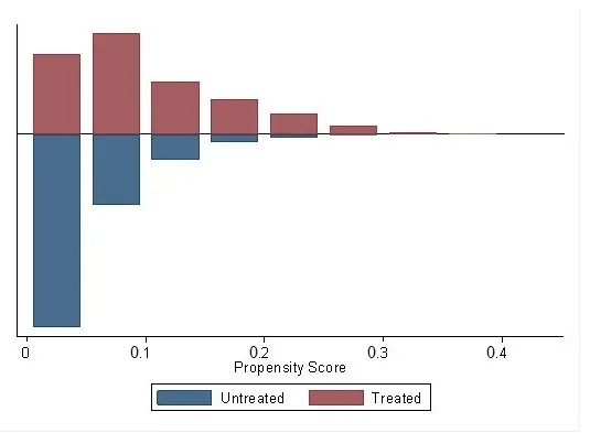
After estimating the propensity scores for each household, a counterfactual group was constructed using radius matching with a caliper of 0.01 for the aggregate sample. As mentioned in the methods section, one of the assumptions to test the matching quality was the conditional independence assumption, which was to ensure that the treatment and control groups had no longer any statistically significant difference in terms of the observable covariates after matching. Before the matching exercise, the treatment and control groups were statistically significantly different in terms of all the covariates except the following: Islam, OBC, never married, divorced/separated, HHH Educational level above primary but up to secondary, Nagaland, West Bengal, Odisha, Gujarat, Daman and Diu, and Andhra Pradesh (Table A2). But the propensity score matching exercise was able to reduce the selection bias in all the covariates as the differences between the treatment and control groups became no longer statistically significant after matching. The mean bias came down from an unmatched 14.5 level to 1.0 level after the matching exercise (Figure A1).
Table A2.
Covariates bias across treated and control groups before and after matching in aggregate sample (radius matching with caliper 0.01).
| Covariates |
Sample |
Mean |
Bias |
t-Test |
| Treated |
Control |
%bias |
%reduced (bias) |
t |
p > |t| |
| Drought yes |
U u |
0.069 |
0.022 |
22.5 |
|
10.03 |
<0.001 |
| M m |
0.069 |
0.072 |
−1.6 |
93.0 |
−0.31 |
0.759 |
| Household size |
U |
5.442 |
4.863 |
23.6 |
|
8.03 |
<0.001 |
| M |
5.442 |
5.491 |
−2.0 |
91.4 |
−0.46 |
0.643 |
| Household with long-term migrant(s) no |
U |
0.761 |
0.733 |
6.3 |
|
2.06 |
0.039 |
| M |
0.761 |
0.764 |
−0.7 |
88.6 |
−0.18 |
0.860 |
| Religion Islam |
U |
0.104 |
0.097 |
2.5 |
|
0.85 |
0.397 |
| M |
0.104 |
0.107 |
−0.9 |
63.0 |
−0.22 |
0.827 |
| Religion Others |
U |
0.030 |
0.060 |
−14.4 |
|
−4.22 |
<0.001 |
| M |
0.030 |
0.032 |
−1.0 |
92.7 |
−0.30 |
0.764 |
| Social group OBC |
U |
0.423 |
0.407 |
3.2 |
|
1.07 |
0.284 |
| M |
0.423 |
0.422 |
0.2 |
94.7 |
0.04 |
0.967 |
| Social group SC |
U |
0.262 |
0.223 |
9.0 |
|
3.05 |
0.002 |
| M |
0.262 |
0.260 |
0.3 |
96.1 |
0.08 |
0.935 |
| Social group ST |
U |
0.182 |
0.099 |
24.0 |
|
9.07 |
<0.001 |
| M |
0.182 |
0.177 |
1.3 |
94.8 |
0.27 |
0.785 |
| Land possession |
U |
1.485 |
1.914 |
−9.8 |
|
−2.71 |
0.007 |
| M |
1.485 |
1.472 |
0.3 |
96.9 |
0.10 |
0.919 |
| Occupation type self-employed in non-agriculture |
U |
0.082 |
0.232 |
−42.1 |
|
−11.98 |
<0.001 |
| M |
0.082 |
0.091 |
−2.6 |
93.8 |
−0.80 |
0.426 |
| Occupation type agricultural labour |
U |
0.164 |
0.137 |
7.8 |
|
2.68 |
0.007 |
| M |
0.164 |
0.160 |
1.1 |
85.8 |
0.26 |
0.797 |
| Occupation type other labour |
U |
0.336 |
0.215 |
27.4 |
|
9.71 |
<0.001 |
| M |
0.336 |
0.341 |
−1.0 |
96.5 |
−0.22 |
0.827 |
| Occupation type others |
U |
0.010 |
0.027 |
−12.3 |
|
−3.45 |
0.001 |
| M |
0.010 |
0.011 |
−0.5 |
96.1 |
−0.15 |
0.880 |
| Income per capita |
U |
13236.000 |
24349.000 |
−32.1 |
|
−8.17 |
<0.001 |
| M |
13236.000 |
13923.000 |
−2.0 |
93.8 |
−0.95 |
0.343 |
| HHH Sex female |
U |
0.081 |
0.144 |
−20.0 |
|
−6.00 |
<0.001 |
| M |
0.081 |
0.084 |
−1.1 |
94.4 |
−0.31 |
0.759 |
| HHH Age |
U |
45.731 |
49.712 |
−29.2 |
|
−9.45 |
<0.001 |
| M |
45.731 |
45.800 |
−0.5 |
98.3 |
−0.12 |
0.901 |
| HHH Marital status never married |
U |
0.005 |
0.010 |
−5.1 |
|
−1.51 |
0.132 |
| M |
0.005 |
0.006 |
−0.9 |
83.0 |
−0.24 |
0.810 |
| HHH Marital status widowed |
U |
0.099 |
0.143 |
−13.5 |
|
−4.19 |
<0.001 |
| M |
0.099 |
0.105 |
−1.9 |
85.9 |
−0.49 |
0.624 |
| HHH Marital status divorced/separated |
U |
0.005 |
0.006 |
−1.3 |
|
−0.41 |
0.684 |
| M |
0.005 |
0.006 |
−1.2 |
2.2 |
−0.30 |
0.765 |
| HHH Educational level literate but up to primary |
U |
0.204 |
0.152 |
13.7 |
|
4.80 |
<0.001 |
| M |
0.204 |
0.203 |
0.3 |
98.2 |
0.06 |
0.954 |
| HHH Educational level above primary but up to secondary |
U |
0.380 |
0.378 |
0.2 |
|
0.07 |
0.942 |
| M |
0.380 |
0.372 |
1.5 |
−603.9 |
0.37 |
0.711 |
| HHH Educational level above secondary |
U |
0.134 |
0.258 |
−31.5 |
|
−9.47 |
<0.001 |
| M |
0.134 |
0.142 |
−1.9 |
94.1 |
−0.51 |
0.609 |
| Himachal Pradesh |
U |
0.006 |
0.048 |
−25.9 |
|
−6.63 |
<0.001 |
| M |
0.006 |
0.009 |
−1.8 |
93.1 |
−0.81 |
0.420 |
| Punjab |
U |
0.016 |
0.047 |
−17.6 |
|
−4.89 |
<0.001 |
| M |
0.016 |
0.019 |
−1.3 |
92.5 |
−0.42 |
0.673 |
| Uttarakhand |
U |
0.004 |
0.011 |
−7.8 |
|
−2.19 |
0.028 |
| M |
0.004 |
0.005 |
−0.9 |
89.0 |
−0.26 |
0.792 |
| Haryana |
U |
0.011 |
0.056 |
−25.2 |
|
−6.64 |
<0.001 |
| M |
0.011 |
0.013 |
−1.2 |
95.3 |
−0.47 |
0.639 |
| Delhi |
U |
|
|
|
|
|
|
| M |
|
|
|
|
|
|
| Rajasthan |
U |
0.086 |
0.068 |
6.6 |
|
2.32 |
0.021 |
| M |
0.086 |
0.083 |
1.0 |
84.7 |
0.24 |
0.814 |
| Uttar Pradesh |
U |
0.127 |
0.095 |
10.3 |
|
3.64 |
<0.001 |
| M |
0.127 |
0.123 |
1.3 |
87.6 |
0.29 |
0.771 |
| Bihar |
U |
0.102 |
0.033 |
27.8 |
|
12.28 |
<0.001 |
| M |
0.102 |
0.109 |
−2.8 |
90.0 |
−0.54 |
0.588 |
| Sikkim |
U |
|
|
|
|
|
|
| M |
|
|
|
|
|
|
| Arunachal Pradesh |
U |
|
|
|
|
|
|
| M |
|
|
|
|
|
|
| Nagaland |
U |
0.001 |
0.003 |
−4.3 |
|
−1.18 |
0.237 |
| M |
0.001 |
0.001 |
−0.6 |
86.0 |
−0.19 |
0.847 |
| Manipur |
U |
|
|
|
|
|
|
| M |
|
|
|
|
|
|
| Mizoram |
U |
|
|
|
|
|
|
| M |
|
|
|
|
|
|
| Tripura |
U |
|
|
|
|
|
|
| M |
|
|
|
|
|
|
| Meghalaya |
U |
|
|
|
|
|
|
| M |
|
|
|
|
|
|
| Assam |
U |
0.016 |
0.028 |
−7.6 |
|
−2.29 |
0.022 |
| M |
0.016 |
0.017 |
−0.1 |
98.2 |
−0.04 |
0.970 |
| West Bengal |
U |
0.044 |
0.048 |
−1.9 |
|
−0.61 |
0.541 |
| M |
0.044 |
0.044 |
0.2 |
91.1 |
0.04 |
0.967 |
| Jharkhand |
U |
0.007 |
0.018 |
−10.1 |
|
−2.84 |
0.005 |
| M |
0.007 |
0.007 |
−0.4 |
95.6 |
−0.14 |
0.888 |
| Odisha |
U |
0.070 |
0.062 |
3.3 |
|
1.12 |
0.261 |
| M |
0.070 |
0.069 |
0.2 |
93.2 |
0.05 |
0.958 |
| Chhattisgarh |
U |
0.067 |
0.039 |
12.3 |
|
4.64 |
<0.001 |
| M |
0.067 |
0.063 |
1.9 |
84.7 |
0.41 |
0.679 |
| Madhya Pradesh |
U |
0.222 |
0.088 |
37.8 |
|
15.34 |
<0.001 |
| M |
0.222 |
0.218 |
1.0 |
97.3 |
0.21 |
0.833 |
| Gujarat |
U |
0.040 |
0.042 |
−0.7 |
|
−0.23 |
0.818 |
| M |
0.040 |
0.037 |
1.5 |
−114.3 |
0.37 |
0.712 |
| Daman and Diu |
U |
0.003 |
0.002 |
2.6 |
|
0.99 |
0.323 |
| M |
0.003 |
0.004 |
−0.2 |
91.0 |
−0.05 |
0.960 |
| Dadra and Nagar Haveli |
U |
|
|
|
|
|
|
| M |
|
|
|
|
|
|
| Maharashtra |
U |
0.046 |
0.091 |
−17.8 |
|
−5.25 |
<0.001 |
| M |
0.046 |
0.045 |
0.4 |
97.8 |
0.12 |
0.908 |
| Andhra Pradesh |
U |
0.050 |
0.046 |
1.6 |
|
0.56 |
0.578 |
| M |
0.050 |
0.050 |
0.2 |
90.8 |
0.04 |
0.971 |
| Karnataka |
U |
0.051 |
0.096 |
−17.5 |
|
−5.18 |
<0.001 |
| M |
0.051 |
0.052 |
−0.5 |
96.9 |
−0.16 |
0.877 |
| Goa |
U |
|
|
|
|
|
|
| M |
|
|
|
|
|
|
| Kerala |
U |
0.003 |
0.028 |
−20.7 |
|
−5.21 |
<0.001 |
| M |
0.003 |
0.004 |
−1.5 |
92.8 |
−0.74 |
0.461 |
| Tamil Nadu |
U |
0.015 |
0.036 |
−12.8 |
|
−3.67 |
<0.001 |
| M |
0.015 |
0.016 |
−0.5 |
96.4 |
−0.14 |
0.887 |
| Pondicherry |
U |
|
|
|
|
|
|
| M |
|
|
|
|
|
|
Figure A1. Distribution of bias. Source: Author’s analysis.
As per the assumption of the common support condition, there should be a region of overlap of the propensity scores between the treatment and control groups after matching. In this study, all of the observations within the treatment group (
i.e., 1162 households) had at least one single observation in the control group within the caliper of 0.01 and hence, no observation in the treatment group remained off support (Figure A2). Therefore, no observation in the treatment group was discarded.
Figure A2. Propensity score distribution. Source: Author’s analysis.
Acknowledgments
I express my sincere acknowledgements to the comments made by Swarup Dutta, Prashant Kumar Singh, Seema Sangita, and Montu Bose throughout the development of this research work.
Ethics Statement
Not applicable.
Informed Consent Statement
Not applicable. The study is based on secondary datasets.
Data Availability Statement
The data underlying the results presented in the study are based on India Human Development Survey (IHDS) second round (2011–12) available at: https://www.icpsr.umich.edu/web/DSDR/studies/36151/datadocumentation.
Funding
The present research is part of a PhD program, which was supported by the University Grants Commission—National Eligibility Test—Junior Research Fellowship (UGC-Ref. No.: 3252/(NET-DEC. 2015)) scheme of the Government of India.
Declaration of Competing Interest
The author has declared that no competing interests exist.
References
-
1.
Adil L, Eckstein D, Künzel V, Schäfer L. Climate Risk Index 2025. Germanwatch e.V. 2025. Available online: https://www.germanwatch.org/sites/default/files/2025-02/Climate%20Risk%20Index%202025.pdf (accessed on 13 June 2025).
-
2.
Mapedza E, McLeman R. Drought risks in developing regions: challenges and opportunities.
Curr. Dire. Water Scar. Res. 2019,
2, 1–14.
[Google Scholar]
-
3.
Panda A. Vulnerability to climate variability and drought among small and marginal farmers: a case study in Odisha, India.
Clim. Dev. 2017,
9, 605–617.
[Google Scholar]
-
4.
Sam AS, Kumar R, Kächele H, Müller K. Quantifying household vulnerability triggered by drought: evidence from rural India.
Clim. Dev. 2017,
9, 618–633.
[Google Scholar]
-
5.
Singh GR, Jain MK, Gupta V. Spatiotemporal assessment of drought hazard, vulnerability and risk in the Krishna River basin, India.
Nat. Hazards 2019,
99, 611–635.
[Google Scholar]
-
6.
Sam AS, Padmaja SS, Kächele H, Kumar R, Müller K. Climate change, drought and rural communities: Understanding people's perceptions and adaptations in rural eastern India.
Int. J. Disaster Risk. Redu. 2020,
44, 101436.
[Google Scholar]
-
7.
Udmale P, Ichikawa Y, Manandhar S, Ishidaira H, Kiem AS. Farmers׳ perception of drought impacts, local adaptation and administrative mitigation measures in Maharashtra State, India.
Int. J. Disaster Risk. Redu. 2014,
10, 250–269.
[Google Scholar]
-
8.
Dallmann I, Millock K. Climate variability and inter-state migration in India.
Cesi. Econ. Stud. 2017,
63, 560–594.
[Google Scholar]
-
9.
Jülich S. Drought triggered temporary migration in an East Indian village.
Int. Migr. 2011,
49, e189–e199.
[Google Scholar]
-
10.
Sarkar B, Dutta S, Singh PK. Drought and temporary migration in rural India: A comparative study across different socio-economic groups with a cross-sectional nationally representative dataset.
Plos. One. 2022,
17, e0275449.
[Google Scholar]
-
11.
Stark O. Research on rural-to-urban migration in LDCs: The confusion frontier and why we should pause to rethink afresh.
World Dev. 1982,
10, 63–70.
[Google Scholar]
-
12.
Stark O, Bloom DE. The new economics of labor migration.
Am. Econ. Rev. 1985,
75, 173–178.
[Google Scholar]
-
13.
Myers N. Environmental refugees: a growing phenomenon of the 21st century.
Philos. Trans. Roya. Soc. Lond., B: Biol. Sci. 2002,
357, 609–613.
[Google Scholar]
-
14.
Piguet E, Kaenzig R, Guélat J. The uneven geography of research on “environmental migration”.
Popu. Environ. 2018,
39, 357–383.
[Google Scholar]
-
15.
Adger WN, Pulhin JM, Barnett J, Dabelko GD, Hovelsrud GK, Levy M, et al. Human security. In Climate Change 2014: Impacts, Adaptation, and Vulnerability. Part A: Global and Sectoral Aspects. Contribution of Working Group II to the Fifth Assessment Report of the Intergovernmental Panel on Climate Change, Field CB, Barros VR, Dokken DJ, Mach KJ, Mastrandrea MD, Bilir TE, et al., Eds.; Cambridge University Press: Cambridge, UK, 2014; pp. 755–791.
-
16.
Bardsley DK, Hugo GJ. Migration and climate change: examining thresholds of change to guide effective adaptation decision-making.
Popu. Environ. 2010,
32, 238–262.
[Google Scholar]
-
17.
Barnett JR, Webber M. Accommodating migration to promote adaptation to climate change. World Bank Policy Research Working Paper No. 5270. 2010. Available online: https://papers.ssrn.com/sol3/papers.cfm?abstract_id=1589284 (accessed on 13 June 2025).
-
18.
Black R, Adger WN, Arnell NW, Dercon S, Geddes A, Thomas D. The effect of environmental change on human migration.
Glob. Environ. Chang. 2011,
21, S3–S11.
[Google Scholar]
-
19.
Black R, Bennett SR, Thomas SM, Beddington JR. Migration as adaptation.
Nature 2011,
478, 447–449.
[Google Scholar]
-
20.
Gemenne F. Migration, a possible adaptation strategy?; IDDRI Report 3. IDDRI: Paris, France, 2010. Available online: https://www.iddri.org/sites/default/files/import/publications/sy_1003_gemenne_migration.pdf (accessed on 13 June 2025).
-
21.
Gemenne F, Blocher J. How can migration serve adaptation to climate change? Challenges to fleshing out a policy ideal.
Geogr. J. 2017,
183, 336–347.
[Google Scholar]
-
22.
McLeman RA, Hunter LM. Migration in the context of vulnerability and adaptation to climate change: insights from analogues.
Wile. Inte. Rev.: Clim. Chang. 2010,
1, 450–461.
[Google Scholar]
-
23.
Sobczak-Szelc K, Fekih N. Migration as one of several adaptation strategies for environmental limitations in Tunisia: evidence from El Faouar.
Comp. Migr. Stud. 2020,
8, 1–20.
[Google Scholar]
-
24.
Vinke K, Bergmann J, Blocher J, Upadhyay H, Hoffmann R. Migration as adaptation?.
Migr. Stud. 2020,
8, 626–634.
[Google Scholar]
-
25.
Gemenne F, Blocher J. How can migration support adaptation? Different options to test the migration–adaptation nexus. In Migration, Environment and Climate Change. Working Paper IOM; IOM: Geneva, Switzerland, 2016.
-
26.
Scheffran J, Marmer E, Sow P. Migration as a contribution to resilience and innovation in climate adaptation: Social networks and co-development in Northwest Africa.
Appl. Geogr. 2012,
33, 119–127.
[Google Scholar]
-
27.
Gilbert G, McLeman R. Household access to capital and its effects on drought adaptation and migration: a case study of rural Alberta in the 1930s.
Popu. Environ. 2010,
32, 3–26.
[Google Scholar]
-
28.
Adger WN, Adams H. Migration as an adaptation strategy to environmental change. In World Social Science Report 2013 Changing Global Environments; OECD Publishing and UNESCO Publishing: Paris, France, 2013; pp. 261–264.
-
29.
Adger WN, Crépin A, Folke C, Ospina D, Chapin FS, Segerson K, et al. Urbanization, migration, and adaptation to climate change.
One. Eart. 2020,
3, 396–399.
[Google Scholar]
-
30.
Tacoli C. Crisis or adaptation? Migration and climate change in a context of high mobility.
Environ. Urban. 2009,
21, 513–525. doi:10.1177/0956247809342182.
[Google Scholar]
-
31.
Hermans K, Garbe L. Droughts, livelihoods, and human migration in northern Ethiopia.
Reg. Environ. Chang. 2019,
19, 1101–1111.
[Google Scholar]
-
32.
Linke AM, Witmer FD, O’Loughlin J, McCabe JT, Tir J. The consequences of relocating in response to drought: human mobility and conflict in contemporary Kenya.
Environ. Res. Lett. 2018,
13, 094014.
[Google Scholar]
-
33.
Ash K, Obradovich N. Climatic stress, internal migration, and Syrian civil war onset.
J. Confl. Reso. 2020,
64, 3–31.
[Google Scholar]
-
34.
IPCC. Climate Change 2022: Impacts, Adaptation, and Vulnerability. Contribution of Working Group II to the Sixth Assessment Report of the Intergovernmental Panel on Climate Change; Pörtner H-O, Roberts DC, Tignor M, Poloczanska ES, Mintenbeck K, Alegría A, Eds.; Cambridge University Press: Cambridge, UK, 2022; p. 3056.
-
35.
Harris JR, Todaro MP. Migration, unemployment and development: a two-sector analysis.
Am. Econ. Rev. 1970,
60, 126–142.
[Google Scholar]
-
36.
Stark O. The Migration of Labor; Basil Blackwell: Cambridge, MA, USA, 1991.
-
37.
Maiti S, Jha SK, Garai S, Nag A, Bera A, Paul V, et al. An assessment of social vulnerability to climate change among the districts of Arunachal Pradesh, India.
Ecol. Indi. 2017,
77, 105–113.
[Google Scholar]
-
38.
Piya L, Maharjan KL, Joshi NP. Vulnerability of rural households to climate change and extremes: Analysis of Chepang households in the Mid-Hills of Nepal. In Proceedings of the International Association of Agricultural Economists (IAAE) Triennial Conference, Foz do Iguaçu, Brazil, 18–24 August 2012.
-
39.
Anderson E, Deshingkar P. Livelihood diversification in rural Andhra Pradesh, India. In Rural Livelihoods and Poverty Reduction Policies, Ellis F, Freeman HA, Eds.; Routledge: London, UK, 2005; pp. 62–81.
-
40.
Angrist JD, Pischke JS. Mostly Harmless Econometrics: An Empiricist’s Companion; Princeton University Press: Princeton, NJ, USA, 2009.
-
41.
Angrist JD, Pischke JS. Mastering’Metrics: The Path from Cause to Effect; Princeton university press: Princeton, NJ, USA, 2014.
-
42.
Banerjee AV, Gertler PJ, Ghatak M. Empowerment and efficiency: Tenancy reform in West Bengal.
J. Political Econ. 2002,
110, 239–280.
[Google Scholar]
-
43.
Wooldridge JM. Introductory Econometrics: A Modern Approach; Cengage learning: Boston, MA, USA, 2015.
-
44.
Banerjee S, Black R, Mishra A, Kniveton D. Assessing vulnerability of remittance‐recipient and nonrecipient households in rural communities affected by extreme weather events: Case studies from South‐West China and North‐East India.
Popu. Space Place 2019,
25, e2157.
[Google Scholar]
-
45.
Deshingkar P. Environmental risk, resilience and migration: implications for natural resource management and agriculture.
Environ. Res. Lett. 2012,
7, 015603.
[Google Scholar]
-
46.
Maharjan A, de Campos RS, Singh C, Das S, Srinivas A, Bhuiyan MRA, et al. Migration and household adaptation in climate-sensitive hotspots in South Asia.
Curr. Clim. Chang. Repo. 2020,
6, 1–16.
[Google Scholar]
-
47.
Singh C, Basu R. Moving in and out of vulnerability: Interrogating migration as an adaptation strategy along a rural–urban continuum in India.
Geogr. J. 2020,
186, 87–102.
[Google Scholar]
-
48.
Srivastava R. Emerging dynamics of labour market inequality in India: Migration, informality, segmentation and social discrimination.
Indian J. Labour Econ. 2019,
62, 147–171.
[Google Scholar]
-
49.
Imbert C, Papp J. Costs and benefits of rural-urban migration: Evidence from India.
J. Dev. Econ. 2020,
146, 102473.
[Google Scholar]
-
50.
Imbert C, Papp J. Short-term migration, rural public works, and urban labor markets: Evidence from India.
J. Eur. Econ. Asso. 2020,
18, 927–963.
[Google Scholar]
-
51.
Chowdhury A, Islam I, Lee D. The Great Recession, jobs and social crises: policies matter.
Int. J. Soc. Econ. 2013,
40, 220–245.
[Google Scholar]
-
52.
Deshingkar P, Sharma P, Kumar S, Akter S, Farrington J. Circular migration in Madhya Pradesh: changing patterns and social protection needs.
Eur. J. Dev. Res. 2008,
20, 612–628.
[Google Scholar]
-
53.
Agarwal S. Urban Migration and Social Exclusion: Study from Indore Slums and Informal Settlements; IIED Working Paper. IIED: London, UK, 2016.
-
54.
Kundu A, Saraswati LR. Migration and exclusionary urbanisation in India.
Econ. Poli. Wkly. 2012,
47, 219–227.
[Google Scholar]
-
55.
Keshri K, Bhagat RB. Temporary and seasonal migration in India.
Genus 2010,
66, 25–45.
[Google Scholar]
-
56.
Keshri K, Bhagat RB. Temporary and seasonal migration: Regional pattern, characteristics and associated factors.
Econ. Poli. Wkly. 2012,
47, 81–88.
[Google Scholar]
-
57.
Esteves T, Rao K, Sinha B, Roy S, Rao B, Jha S, et al. Agricultural and livelihood vulnerability reduction through the MGNREGA.
Econ. Poli. Wkly. 2013,
48, 94–103.
[Google Scholar]
-
58.
Jha CK, Gupta V, Chattopadhyay U, Amarayil Sreeraman B. Migration as adaptation strategy to cope with climate change: A study of farmers’ migration in rural India.
Int. J. Clim. Chang. Strateg. Manag. 2018,
10, 121–141.
[Google Scholar]
-
59.
Rodgers G, Rodgers J. Inclusive development? Migration, governance and social change in rural Bihar.
Econ. Political Wkly. 2011,
46, 43–50.
[Google Scholar]
-
60.
Deshingkar P. Improved livelihoods in improved watersheds: Can migration be mitigated? In Proceedings of the International Workshop on Watershed Management Challenges, New Delhi, India, 3–4 November 2004.
-
61.
Reardon T, Berdegué J, Barrett CB, Stamoulis K. Household income diversification into rural nonfarm activities. In Transforming the Rural Nonfarm Economy: Opportunities and Threats in the Developing World; Haggblade S, Hazell PBR, Reardon T, Eds.; International Food Policy Research Institute: Baltimore, MD, USA, 2007; pp. 15–140.
-
62.
Sarkar B. Migration in the Drought-Affected Rural Areas in India: An Exploratory Study. [Doctoral dissertation, TERI School of Advanced Studies]. Shodhganga: A reservoir of Indian theses @ INFLIBNET. 2024. Available online: https://shodhganga.inflibnet.ac.in/handle/10603/601915 (accessed on 13 June 2025).
-
63.
Rosenbaum PR, Rubin DB. Constructing a control group using multivariate matched sampling methods that incorporate the propensity score.
Am. Stat. 1985,
39, 33–38.
[Google Scholar]
-
64.
Rosenbaum PR, Rubin DB. The central role of the propensity score in observational studies for causal effects.
Biometrika 1983,
70, 41–55.
[Google Scholar]
-
65.
Caliendo M, Kopeinig S. Some practical guidance for the implementation of propensity score matching.
J. Econ. Surv. 2008,
22, 31–72.
[Google Scholar]
-
66.
Heinrich C, Maffioli A, Vazquez G. A Primer for Applying Propensity-Score Matching; Inter-American Development Bank, Impact-Evaluation Guidelines, Technical Notes No. IDB-TN-161. Office of Strategic Planning and Development Effectiveness (SPD): Dubai, UAE, 2010.
-
67.
Leuven E, Sianesi B. PSMATCH2: Stata Module to Perform Full Mahalanobis and Propensity Score Matching, Common Support Graphing, and Covariate Imbalance Testing; Statistical Software Components S432001, Boston College Department of Economics. 2003. Available online: http://ideas.repec.org/c/boc/bocode/s432001.html (accessed on 13 June 2025).