1. Introduction
The global meat industry has been dominated by poultry production, with both the output and consumption of poultry products exhibiting significant growth [
1,
2]. In recent years, the demand for chicken in consumer markets has steadily increased, and global chicken consumption is projected to exceed 104.9 million tonnes by 2025. Compared to other types of meat, chicken offers advantages such as a short production cycle, cost-efficiency, and balanced nutrition, making it an increasingly preferred protein source for households. The growing consumer preference for high-protein, low-fat foods has further accelerated the expansion of the poultry consumption market.
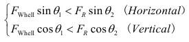
Machine vision technology has been widely applied in the quality inspection and grading of broiler carcasses. Particularly during the slaughtering stage, carcass grading using machine vision is crucial for ensuring product quality consistency and maintaining market competitiveness. Traditional manual weighing methods are not only inefficient but also pose a risk of secondary contamination. In response, the team led by Chen Kunjie [
3,
4] at Nanjing Agricultural University proposed a broiler carcass quality grading method based on machine vision technology. This method captures carcass feature information using digital and depth cameras, extracts key parameters such as projected area, contour length, and breast width through image preprocessing, and constructs nonlinear mathematical models to achieve non-contact automatic grading of broiler carcasses (as shown in ). Additionally, the team employed CT scanning technology to capture the physical features of Sanhuang broiler carcasses and accurately calibrate the locations of major internal organs, providing essential data support for the development of robotic retrieval and automated evisceration devices. The research team led by Professor Ding Xiaoling [
5] at Shandong Agricultural University focused on predicting the quality of chicken wings and proposed a rapid, non-destructive external quality detection model. This approach involved acquiring top and side-view images of 140 chicken wings, processing them through grayscale transformation and morphological operations, and extracting key features such as area, contour perimeter, major axis, and minor axis. Actual dimensions were calculated through camera calibration, and univariate linear, exponential, and multivariate hybrid prediction models were developed to enable the automatic grading of chicken wing quality. Building on these findings, the team further developed a chicken wing grading and packaging device, advancing automation in processing and significantly improving production efficiency. Zhuang Chao [
6] proposed a body weight prediction method combining neural networks with machine vision, using depth cameras to capture infrared and depth images of white-feather broilers. Target identification was performed using the YOLOv3 algorithm, and convolutional neural networks were employed for image segmentation to construct a model for extracting broiler regions. Innocent Nyalala [
7] designed a carcass weight prediction system based on depth images, segmenting the carcass into five parts—drumsticks, breast, wings, head, and neck—using the Active Shape Model (ASM). Key point detection was used to determine cutting lines, refining the segmentation precision of each part and enhancing processing efficiency.
During broiler carcass processing, issues such as damage, broken wings, hemorrhages, and inflammation frequently occur. The team led by Professor Wang Huhu [
8,
9,
10] at Nanjing Agricultural University developed a three-station visual acquisition device capable of rapidly capturing broiler carcass images from multiple angles. Features such as skin color arrays and area distribution were extracted, and defects were intelligently identified and predicted through traditional linear analysis combined with machine learning, forming a machine vision-based detection framework. Tran M [
11] proposed a more advanced end-to-end architecture called the Carcass Former, leveraging powerful computational resources to locate, analyze, and classify poultry carcass defects while also detecting minor imperfections such as residual feathers, thereby significantly improving overall recognition accuracy. The Intelligent Equipment team at Wuhan Polytechnic University [
12,
13] focused on the research of automated evisceration, leveraging machine vision-captured data to explore body part recognition, optimization of bionic motions during the evisceration process, and mechanical posture prediction. They successfully achieved design goals for cavity opening determination, inference of organ distribution, and touch-signal-driven fine adjustment of hand shapes, completing the integration and assembly of the corresponding hardware systems. By integrating deep learning with mechanical theories and through a series of experiments, they achieved precise recognition and cutting of key parts such as chicken wings and drumsticks, providing technical support for precision poultry processing. Cai Lu explored the application of 3D point cloud and machine vision technologies in poultry carcass cutting, predicted abdominal curves, organ locations, and sizes, and applied industrial robotic precision cutting technologies to enhance segmentation accuracy.
Although previous studies have explored image segmentation and quality prediction for broiler carcasses, they still face several limitations. Existing segmentation models often lack robustness under complex backgrounds, and many prediction methods rely on limited handcrafted features with poor generalization. Moreover, few studies consider the mapping between image features and physical measurements, limiting their practical applicability.
This study aims to address these gaps by proposing an integrated machine vision system for broiler carcass evaluation. We formulate the following scientific hypotheses: (1) morphological features (e.g., breast area, axis length) is significantly correlated with carcass weight; (2) the improved YOLOv8n-seg model with an ADown module enhances segmentation accuracy in practical settings; (3) CNN-based regression models outperform traditional methods in predictive performance; (4) This research not only verifies the performance of the model, but also proposes the design scheme of the actual production line.
The main contributions of this work include: (a) a lightweight and high-accuracy segmentation model optimized with the ADown module; (b) a calibrated feature extraction method combining HSV color space, convex hull, and dynamic ellipse fitting; (c) an end-to-end prediction framework integrating deep learning and traditional regression to improve quality estimation accuracy.
. Quality and quality detection of broilers based on machine vision.
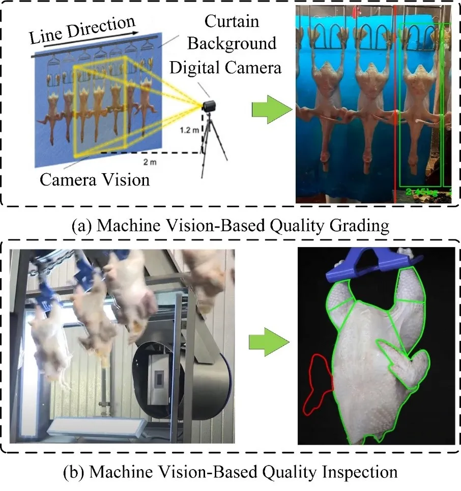
The development of poultry carcass segmentation technology has entered a fully automated stage (As shown in ). Leading companies such as Meyn (The Netherlands) and Baader (Denmark) have integrated machine vision, real-time dynamic weighing components, and AI recognition systems to create closed-loop, highly adaptive segmentation production lines. For instance, Meyn’s Flex Plus employs a vision-based system capable of dynamically recognizing anatomical parts based on color and structure, enabling seamless integration between precise grading and deboning operations. The system stands out not only for its operational efficiency but also for its versatility in handling various product specifications, reflecting the maturity of its design philosophy and breadth of application. Baader has adopted a continuous learning approach that fuses artificial intelligence with a visual inspection, steadily improving segmentation accuracy and ensuring consistent, high-quality inspection across diverse poultry types. The integration of robotics and machine vision has become a primary direction in advancing intelligent poultry processing, effectively addressing challenges posed by morphological variability and inconsistent soft tissue elasticity—issues that have garnered significant attention in both domestic and international research.
Addressing the practical needs of poultry carcass segmentation, Hu [
14] et al. combined statistical analysis with image processing techniques to propose a concept for poultry shoulder joint cutting and developed an initial system architecture. Early results indicated significant potential in reducing labor costs and enhancing processing speed. In the field of chicken tender harvesting, Misimi [
15] et al. developed the GRIBBOT robotic system, which integrates 3D vision-guided technology for automated tender harvesting. The system uses vision algorithms to determine optimal grasping points and employs customized grippers to detach tenders from the skeleton, enabling full automation. Experimental results demonstrated that the system can accurately perform chicken tender harvesting tasks. Konrad Ahlin [
16] et al. proposed the application of robotic technologies in poultry processing lines, enabling functions such as automated hanging, robotic deboning, and adaptive gripping. This solution overcomes the rigidity of traditional production lines. Robotic workstations can perform all necessary operations without relying on fixed cutting equipment, allowing for more efficient intelligent decision-making and dynamic adjustment of production strategies based on real-time product feedback to achieve optimal yield for each individual item.
. Poultry intelligent segmentation equipment.
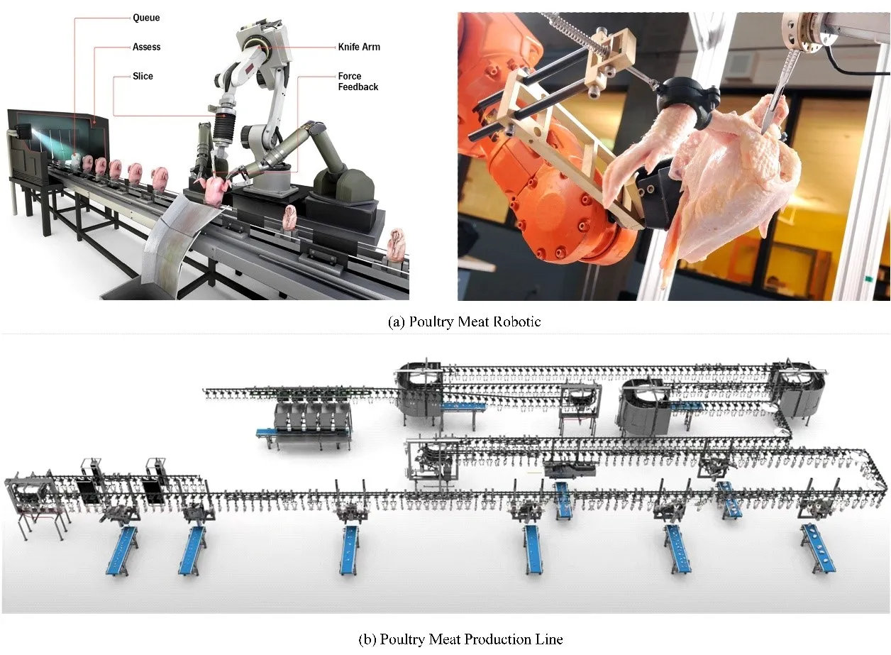
illustrates the development trajectory of poultry processing equipment and machine vision technologies, clearly depicting the transition from traditional processing methods to modern intelligent production. In poultry processing, cutting is a core operation, and its efficiency is closely tied to overall product quality. Many large enterprises have established comprehensive automated production lines, significantly reducing contamination and error risks associated with manual operations and steadily improving product quality consistency.
. Machine Vision in Broiler Inspection and Automated Processing.
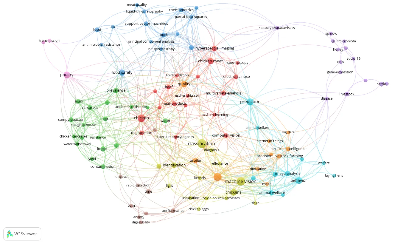
Additionally, a keyword analysis based on a search in the Web of Science database reveals the research hotspots in poultry processing equipment and machine vision, as shown in . The search was conducted using the terms “poultry processing equipment” and “machine vision”. The size of each dot indicates the frequency of keyword occurrence in the literature—the larger the dot, the greater the research interest. Machine vision has been widely applied in poultry processing, food quality control, and livestock health monitoring, with research hotspots becoming increasingly focused in recent years.
. Distribution of hot spots in poultry processing and detection.
2. YOLOv8-Seg Image Segmentation Algorithm for Broiler Carcasses
2.1. YOLOv8-Seg Network
As an extended model of the YOLOv8 series, YOLOv8-seg introduces structural improvements and optimizations, specifically for instance, segmentation tasks. It demonstrates strong performance in various applications, including traffic sign segmentation in autonomous driving, tissue region identification in medical imaging, and object classification and segmentation in industrial environments. Compared to the standard YOLOv8 [
17,
18], YOLOv8-seg integrates a mask segmentation mechanism, enabling the system to perform beyond basic object detection. In particular, it can generate fine-grained object contour information, making it better suited for applications that demand high precision in local detail representation.
2.2. ADown
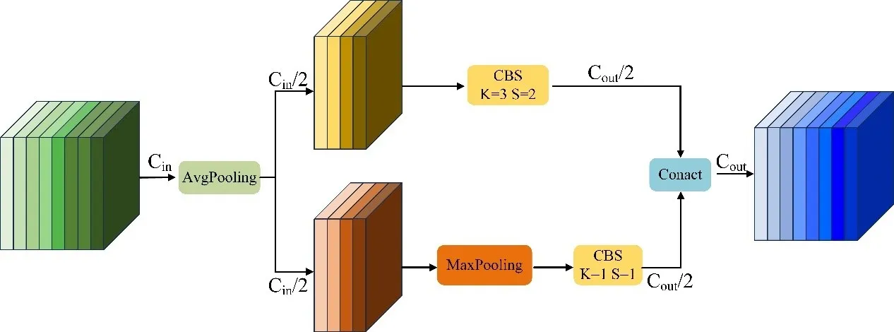
The ADown downsampling process consists of two branches: a 1 × 1 branch and a 3 × 3 branch. The input feature map is first processed by a 2 × 2 average pooling layer and then split along the channel dimension into two sub-feature maps,
X1 and
X2.
X1 is processed through the 3 × 3 branch, where the number of channels is adjusted to Cout/2 (where Cout represents the number of output feature channels [
19]. The
X2 feature map is processed through the 1 × 1 branch, where it first undergoes a max pooling layer to extract local maxima, followed by a convolutional layer to perform downsampling. This design not only achieves lightweight downsampling but also better preserves critical feature information. Finally, the output feature maps from both branches are merged through a concatenation (concat) operation to form the final output.
In this study, the convolutional downsampling modules in both the backbone and neck of the network were replaced with lightweight ADown modules (as shown in
). This design, utilizing a branched structure, provides richer feature information, reduces the loss of fine details, and maximally preserves key features while maintaining a low parameter count and computational burden.
. ADown downsampling structure.
The output feature map of global average pooling is computed according to the following formula:
Here, $$k$$ represents the size of the pooling kernel and $$s$$ represents the pooling stride (usually $$k$$ =$$s$$), which defines the coordinates of the pooled feature map. Global average pooling performs average pooling on the feature map, averaging the values within each $$k$$×$$k$$ region to generate a lower-frequency feature map. Average pooling smooths the feature map, reduces high-frequency noise, and is beneficial for extracting global information from the entire image. The computation formula for max pooling is as follows:
The operation preserves significant information in the feature map, especially the edge or texture features. Maximum pooling is applied to the split $$X_{2}$$ feature map, where the maximum value is taken from each $$k$$×$$k$$ region.
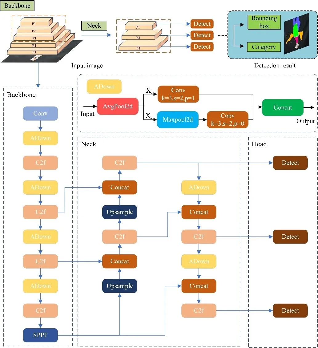
After embedding the ADown technique into the backbone and neck networks of YOLOv8, the model shows a significant improvement in feature extraction and fusion capabilities, especially in multi-scale object detection. The ADown method introduces a learnable attention mechanism, allowing the network to dynamically adjust the downsampling method based on input features, selectively retaining core features while minimizing the risk of information loss, resulting in more precise and effective detection. The improved lightweight YOLOv8n-seg network structure is shown in
.
. YOLOv8n-seg-Adown network structure diagram.
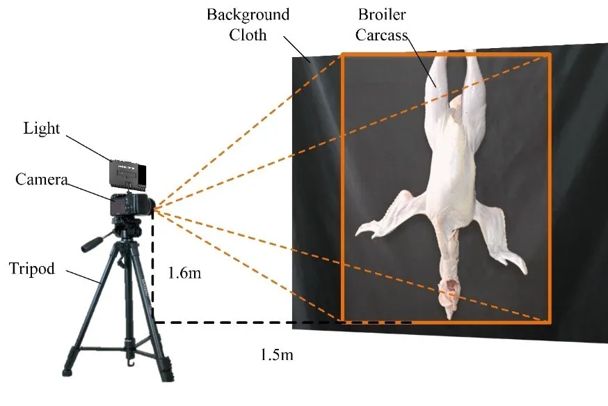
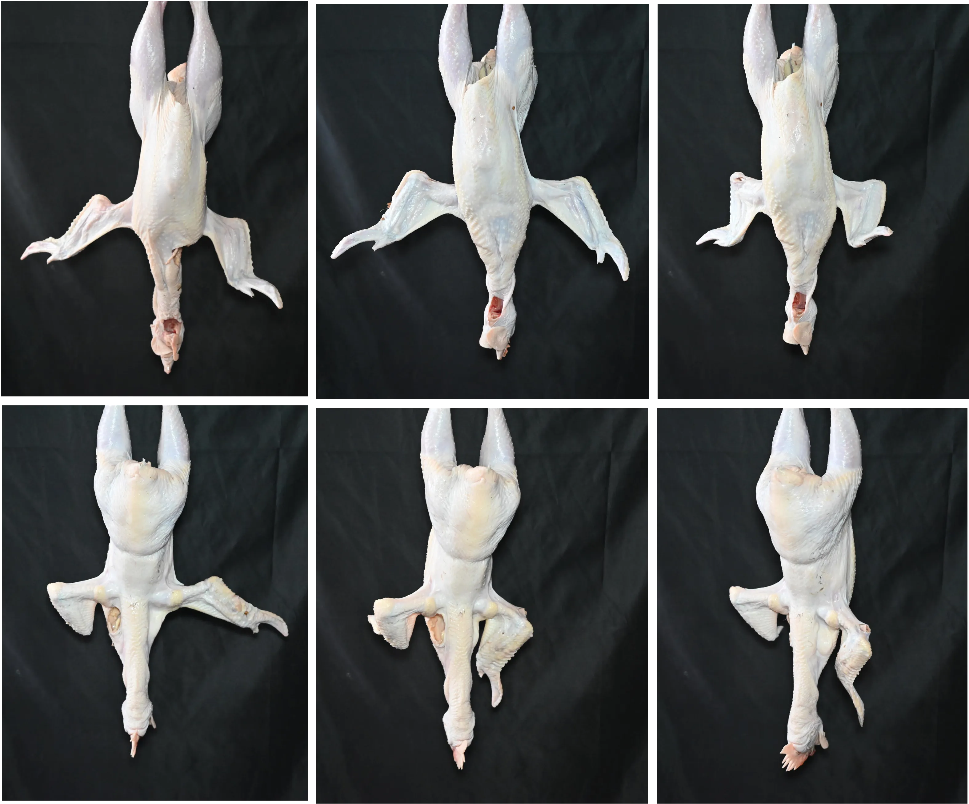
The chicken carcass images utilized in this study were acquired at a poultry slaughterhouse located in the Huangdao District of Qingdao City between 24 and 26 October 2024. The imaging equipment consisted of a Nikon D90 single-lens reflex camera with a resolution of 4288 × 2848 pixels, equipped with a 35 mm prime lens. The lighting conditions featured an 8 W power source and a color temperature of 6800 K. To minimize interference from the complex background, a black backdrop was employed during image capture. The camera was positioned 1.5 m away from the chicken carcasses, with the lens set to a focal length of 35 mm, the aperture adjusted to F6, and the optical axis height maintained at 1.6 m. During data collection, three distinct breeds of chicken carcasses (a total of 165 samples) were selected from the slaughterhouse. Following image acquisition, the weight of each chicken carcass was measured using an electronic scale with an accuracy of ±0.01 kg, and each sample was assigned a unique identifier.
This study focuses on the collection and analysis of chicken carcass images. To simulate the hanging conveyance in actual production, the experimental platform was designed to collect images with a double-leg hanging posture (as shown in
). To build a training dataset for chicken carcass image segmentation and detection, an image collection system was established, consisting of a digital camera, camera mount, supplemental lighting, and a hanging apparatus.
. The image acquisition setting and site environment.
To simulate the state of the chicken carcasses on a hanging conveyor line, the carcasses were suspended on a rack. Under the influence of gravity, the carcasses naturally droop, with the chest positioned perpendicular to the camera’s optical axis. The digital camera was mounted on a tripod 1.6 m away from the chicken carcasses to ensure the complete capture of the carcass images. A black background cloth was set to minimize image noise (as shown in
).
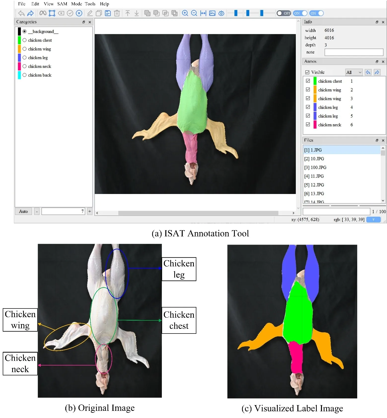
This study introduced the open-source tool ISAT for performing image annotation tasks (as shown in
). This tool integrates the latest predictive capabilities of the SAM model to assist the annotation process, significantly reducing labor costs and improving annotation efficiency [
20,
21,
22]. Compared to traditional methods, ISAT demonstrated superior segmentation accuracy and adaptability across multiple datasets, improving annotation levels. The processing time for a single image was reduced from 45 s to 12 s, achieving a speedup of 3.7 times.
. ISAT annotation tool interface.
After filtering out blurred and incomplete images, 1000 chicken carcass images were obtained for annotation and detection. These images were randomly collected from a slaughterhouse and then divided into training, validation, and test sets. The specific annotation interface is shown in
, covering six categories: background (cls0, black), chicken chest (cls1, green), chicken wings (cls2, yellow), chicken legs (cls3, purple), chicken neck (cls4, red), and chicken back (cls5, blue). The original images are in 24-bit RGB format, with annotations made based on body parts, but due to unclear boundaries, the annotations were manually adjusted by dragging blocks to ensure accuracy.
2.4. Experimental Analysis
To verify the practical effects of introducing the ADown module and conducting an ablation experiment, the structure is shown in
.
.
Ablation experiment comparison.
| Index |
DWconv |
ADown |
mAP@0.5/% |
Parameters (M) |
FLOPs (G) |
Model Size (M) |
| Box |
Mask |
| 1 |
|
|
0.993 |
0.991 |
3.3 |
12.0 |
12.90 |
| 2 |
√ |
|
0.985 |
0.989 |
3.1 |
11.5 |
5.70 |
| 3 |
|
√ |
0.992 |
0.994 |
2.8 |
11.1 |
5.39 |
Where ADown and DWconv represent the two improved modules. After incorporating the ADown module, the model’s accuracy remained stable (the mAP@0.5 box indicators were 99.2% and 99.4%, with similar mask values). The lightweight performance was remarkable: parameters were compressed to 2.8 M, a reduction of 0.5 M; floating point operations decreased to 11.1 G, reducing by 0.9 G, and weight capacity was reduced to 5.39 M, a reduction of 7.51 M from the original scale.
To further evaluate the practical performance of the improved YOLOv8s algorithm in broiler carcass segmentation tasks, this study compared it with other YOLO series algorithms, including YOLOv5s-seg, YOLOv8n-seg, and YOLOv9c-seg, under identical experimental conditions.
As shown in
, compared with YOLOv5s-seg and YOLOv9c-seg, the improved YOLOv8n-seg model shows little difference in mAP@0.5 (box) and mAP@0.5 (mask) performance, but achieves significant reductions: the number of parameters decreased by 4.6 M and 24.8 M, the floating-point operations (FLOPs) reduced by 14.6 G and 146.6 G, and the model weights shrank by 9.01 M and 48.21 M, respectively. As shown in
, compared with YOLOv5s-seg and YOLOv9c-seg, the improved YOLOv8n-seg model shows little difference in mAP@0.5 (box) and mAP@0.5 (mask) performance, but achieves significant reductions: the number of parameters decreased by 4.6 M and 24.8 M, the floating-point operations (FLOPs) reduced by 14.6 G and 146.6 G, and the model weights shrank by 9.01 M and 48.21 M, respectively. The lightweight design significantly reduces resource consumption, making the model better suited for embedded devices with limited computational power. It achieves a favorable balance between recognition accuracy and response speed, aptly meeting practical application requirements and becoming the preferred choice for broiler carcass segmentation tasks.
.
Model performance comparison.
| Index |
mAP50 |
Map50-95 |
Parameters (M) |
FLOPs (G) |
Model Size (M) |
| Box |
Mask |
BOX |
Mask |
| Yolov5s-seg |
0.991 |
0.994 |
0.884 |
0.907 |
7.4 |
25.7 |
14.4 |
| Yolov8n-seg |
0.993 |
0.991 |
0.882 |
0.903 |
3.3 |
12.0 |
12.9 |
| Yolov9c-seg |
0.985 |
0.993 |
0.906 |
0.912 |
27.6 |
157.7 |
53.6 |
Yolov8n-
ADown-seg
|
0.992 |
0.994 |
0.875 |
0.896 |
2.8 |
11.1 |
5.4 |
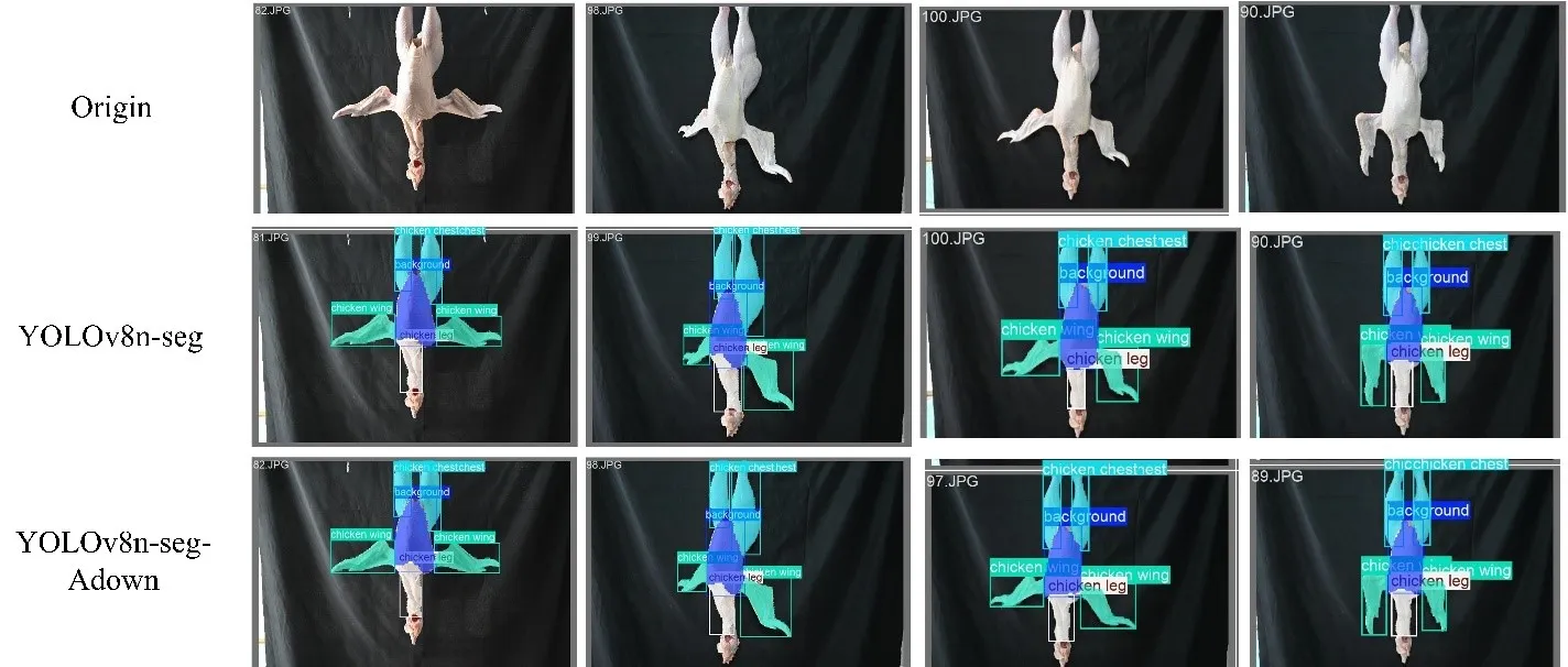
To compare the performance of the improved YOLOv8n-seg model with the original YOLOv8n-seg in practical segmentation tasks, a subset of images from the validation set was selected for comparison. The segmentation results are presented in
.
. Visualization of segmentation results.
Although both models showed some differences in mask overlap when handling different regions, neither exhibited missing detections or misclassifications. For frontal images of broiler carcasses, both models could accurately segment the target areas from the background. However, under side-view conditions, when the wings overlapped with the breast area, the original model demonstrated certain weaknesses, such as incomplete object segmentation and cluttered masks in occluded areas. In contrast, the improved model exhibited finer discrimination in such cases, with better handling of overlapping regions and overall more optimized results.
3. Methods for Processing Chicken Carcass Characteristics
In the field of digital image processing, extracting meaningful features from raw images has always been a challenging task. Taking broiler carcass feature analysis as an example, separating the carcass from the background environment and accurately locating the breast region poses significant challenges. Traditional methods often encounter instability when dealing with complex backgrounds and irregular targets. In this study, HSV color space-based image segmentation was employed to extract overall features such as the area and perimeter of broiler carcasses. Subsequent optimization of the segmentation results further improved the accuracy of feature extraction. For breast region analysis, contour detection using ellipse fitting and convex hull algorithms enabled precise measurement of the breast area as well as the major and minor axes. By comparing the results obtained from different methods against benchmark data, the most optimal feature extraction approach was selected to ensure both the reliability and accuracy of the findings.
3.1. Mechanism of Feature Processing Methods
3.1.1. HSV
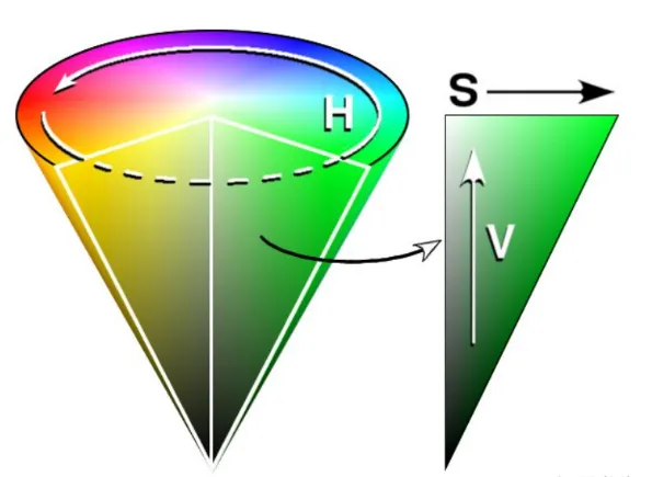
The HSV color space has been widely adopted in digital image processing due to its intuitive representation [
23,
24]. This model maps the RGB color space into an inverted cone (as shown in
), where H represents hue, S denotes saturation, and V corresponds to value (brightness). Such a decomposition separates color information independently, facilitating color analysis and processing, and is particularly effective for image segmentation. During the broiler carcass image processing, distinct color differences between various parts of the mask were observed. Utilizing the HSV color space enabled more precise color segmentation, laying a solid foundation for subsequent feature extraction. In this study, the segmented RGB images were first converted into HSV format, and each color component was thoroughly analyzed to enhance the accuracy of both mask segmentation and feature extraction.
The conversion formula for the HSV color space is as follows:
3.1.2. Convex Hull
In machine vision, color extraction techniques can generate an initial mask for the chicken breast region, which can be directly utilized [
25,
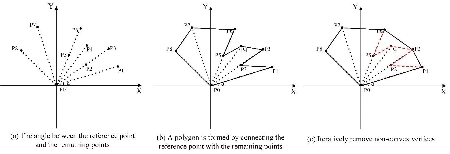
26]. However, issues such as rough or broken edges often arise, posing challenges for the subsequent extraction of geometric features like major and minor axes. To address this, the convex hull algorithm was employed to optimize the mask region acquisition. The detailed procedure is illustrated in
. According to the definition of convex combinations:
the convex hull is the smallest convex boundary formed by the convex combination of all points in a given set.
Subsequently, taking a reference point, the other points are sorted in ascending order based on their polar angles. The method for calculating the polar angle is as follows:
After sorting, the convexity of the point set is checked point by point, starting from the second point. The vector cross-product is used to determine whether the current point forms a “left turn”, and the cross-product formula is as follows:
If the cross product Cross > 0, the current point forms a left turn and satisfies the convex hull condition, and thus is added to the convex hull; if Cross ≤ 0, the point does not meet the convex hull condition (right turn or collinearity), and the last point in the hull is removed.
After traversing all points, the algorithm outputs the minimum convex hull encompassing all points. Its area can be calculated using the following formula:
. Convex hull detection process.
3.1.3. Ellipse Fitting
The chicken breast region is critical in broiler carcasses, accounting for approximately 58% to 75% of the total mass [
27,
28]. Its economic value is significant, and it also directly reflects the overall geometric properties of the carcass. When extracting geometric features of the chicken breast, the focus is on dimensional measurements along the vertical and horizontal directions, which are crucial for processing precision and quality prediction. The initial estimation formula for the ellipse center is as follows:
Here, $$x_{i} , y_{i}$$ represent the coordinates of the $$i$$ boundary point, and $$N$$ is the total number of boundary points. By calculating the mean values of all boundary points along the horizontal and vertical directions, the estimated geometric center $$( x_{c} , y_{c} )$$can be obtained.
This study introduces a weighted point density optimization strategy, where boundary points near the major axis are assigned higher weights while the influence of distant points is diminished [
29]. The specific optimization formula is as follows:
Here, $$w_{i}$$ denotes the weight of the $$i$$ -th point; dist(
xi,long_axis) represents the distance from that point to the ellipse’s major axis; and $$\sigma$$ is the Gaussian control parameter that determines the rate at which the weight decays with distance. A larger $$\sigma$$ implies a slower decay of point weights.
After determining the center point, the most appropriate ellipse needs to be fitted based on the center. In the polar coordinate system, the ellipse equation can be expressed as:
Here, $$x \left( t \right) , y \left( t \right)$$ represents the coordinates of a point on the ellipse; $$a , b$$ denotes the lengths of the ellipse’s major and minor axes; $$\theta$$ is the rotation angle of the ellipse (the angle with the horizontal axis); and $$t$$ is the ellipse parameter (with a value range of $$t \in \left[0 , 2 \pi\right]$$).
The initial estimation method has limitations in accuracy and the complex distribution of boundary points. To improve this situation, this paper introduces dynamic parameter adjustment to enhance the ellipse fitting effect. Specifically, the gradient descent method is used to update parameters related to the ellipse’s center, major axis, minor axis, and rotation angle. During this process, the objective function is constructed using a weighted least squares method to serve the subsequent optimization process, defined as:
Here, $$d \left( e_{o} \right)$$ represents the weighted average distance of all boundary points to the ellipse, and $$x_{i} , y_{i}$$ are the coordinates of the boundary points. In this process, by continuously adjusting the learning rate and gradient direction, the parameter updates are made both rapidly and stably, achieving more accurate ellipse fitting. The parameter adjustment is based on the gradient descent method, which updates the parameters by calculating the gradient of the objective function. The iterative update formula is:
Here, $$\theta_{t + 1} , \theta_{t}$$ represents the set of ellipse parameters after and before iteration, including $$\left( x_{c} , y_{c} , a , b , \theta \right)$$, $$\eta$$ represents the learning rate, which controls the step size of the iteration, $$\nabla d \left( e_{o} \right)$$ represents the gradient of the objective function, and indicates the direction and magnitude of parameter adjustment. During the iteration process, a geometric constraint $$4 A C - B^{2} > 0$$ is added to ensure that the fitting result conforms to the mathematical properties of an ellipse rather than a hyperbola or parabola.
Finally, the optimization scheme evaluates the fitting result through coverage validation, and the calculation formula for coverage is as follows:
3.2. Extraction of Broiler Carcass Features
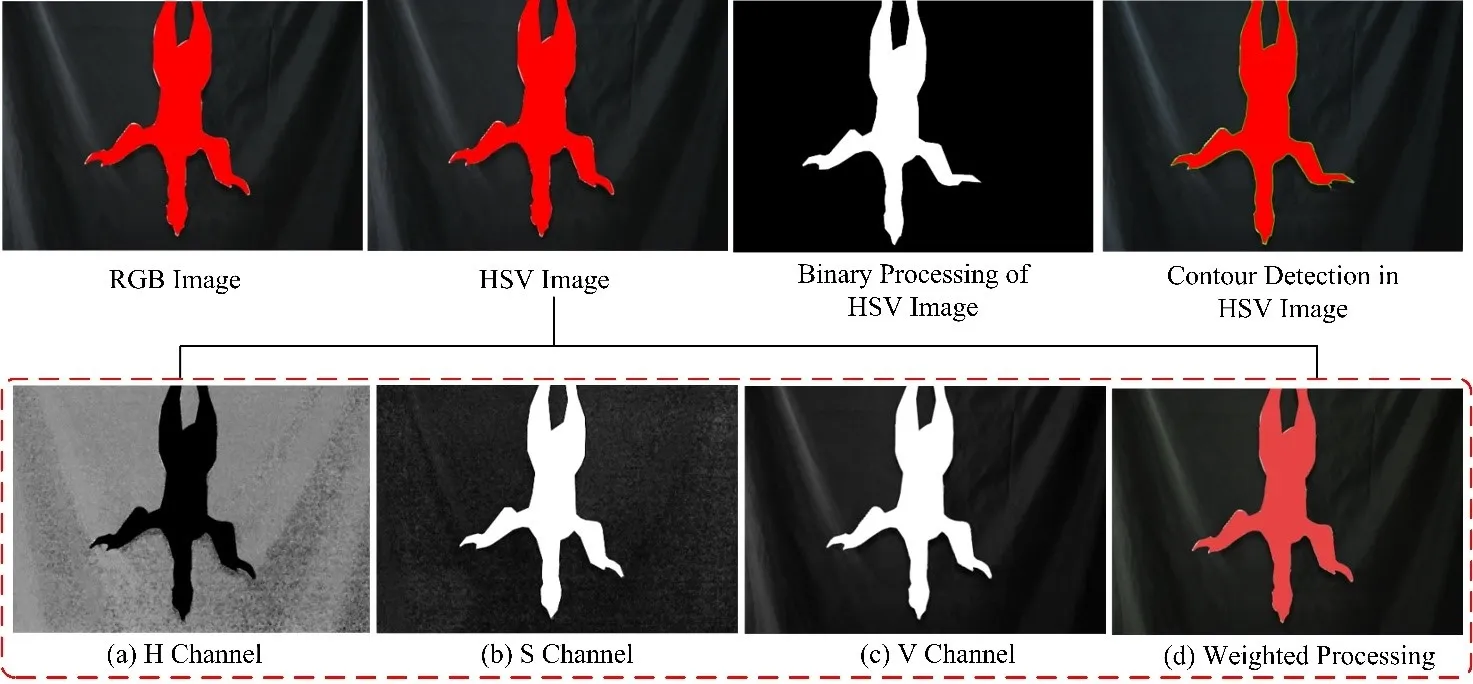
This study uses image segmentation to extract the red region of the whole chicken carcass and then performs detailed measurements of its area and contour features (as shown in ). The specific process is as follows: the original RGB image is first converted to the HSV color model. Using hue, saturation, and brightness, the red region of the chicken carcass is distinguished. In the HSV space, red is primarily scattered in two specific intervals: one is the low-value range from [0,120,70] to [10,255,255], and the other is the high-value range from [170,120,70] to [180,255,255]. After generating binary masks for these two intervals, the masks are combined using the “OR” logical operation to obtain the complete red region mask.
. Process for feature extraction of broiler carcass based on HSV color space.
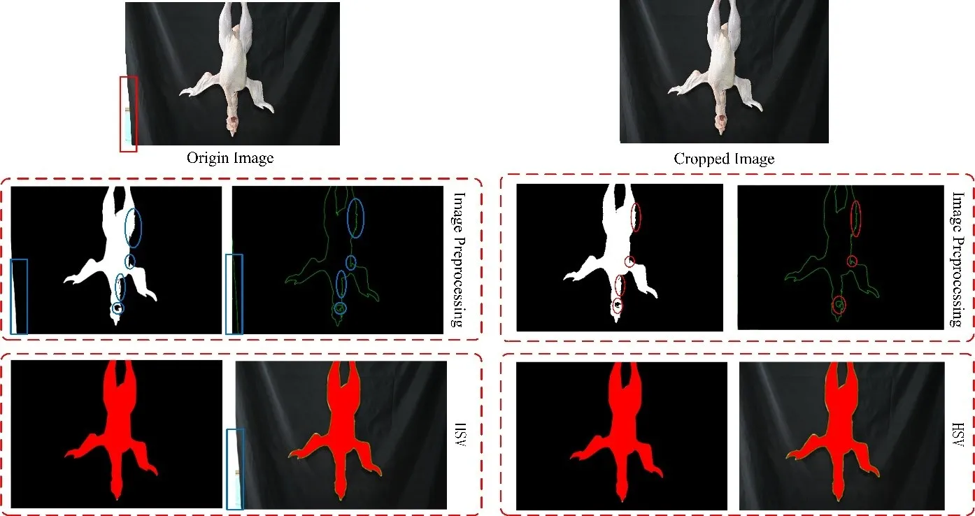
In the actual shooting process, the background layout was not ideal, and external scenes accidentally entered the frame, affecting the image preprocessing. In the original image, the external background area in the lower-left corner, marked by the red box in
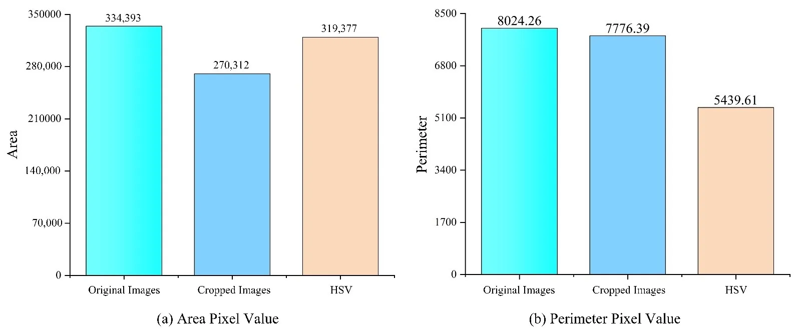
, was misjudged as the target area. The calculated area reached 334,393 pixels, and the perimeter was 8024.26 pixels. Additionally, the neck wound and the uneven height of the chicken wings and breast caused shadowing issues, increasing the uncertainty in the region’s resolution.
To reduce background interference, the image was cropped to eliminate excess external background, making the target area more focused and clear. In the cropped image, the recognizability of the target area was significantly improved, with the area and perimeter adjusted to 270,312 pixels and 7776.39 pixels, respectively. Although cropping effectively reduced background noise, the shadowing issues caused by the neck wound and height differences still existed, resulting in some errors in the calculated results. Therefore, further improvements to the algorithm are needed in the future to enhance the accuracy of image segmentation and feature extraction.
. Comparison of area and perimeter pixel points of broiler carcass.
shows the comparison data of area and perimeter obtained under different processing methods. After the segmentation, the image was processed in the HSV color space. The study successfully extracted the red mask area of the whole chicken with precise region localization. The method eliminates the influence of the external environment from the original image. In the cropped image, the same technique calculated the area as 319,377 pixels and the perimeter as 5439.61 pixels, with both data matching the original image, demonstrating the stability of the HSV color space under different shooting conditions.
. Comparison of area and perimeter pixel points of broiler carcass.
This study uses image processing and ellipse fitting to conduct a quantitative analysis of the area and geometric properties of the chicken’s breast. First, image preprocessing, morphological operations, and image segmentation were used to extract the chicken breast region. Then, ellipse fitting was applied to the target area, obtaining the values of the ellipse’s major and minor axes, which were used as parameters for the geometric characteristics of the chicken’s breast.
In this paper, an external rectangle operation was applied to the chicken breast mask area in the annotated image (as shown in
), and its length and width were calculated. Since the chicken images in this study are in a vertically hanging state, the obtained length and width values can be used as reference parameters for consideration.
. Bounding rectangle of broiler breast mask.
In the evaluation stage, the green mask area shown in the image marked in was used as the standard value for the chicken breast area, while the length and width of the green mask external rectangle in were used as the reference for the major and minor axes. By comparing the results extracted by different methods, their accuracy and reliability in calculating the chicken breast area and geometric features can be evaluated.
This study researched the image segmentation mask. First, the manually labeled chicken breast mask was converted into the HSV color space. The extracted area was 106,997 pixels, and ellipse fitting showed that the corresponding covered area was 110,484 pixels. The axial data were 561.34 and 250.60 pixels, respectively. After convex hull operation, the area was updated to 110,609 pixels. After further ellipse fitting, the area expanded to 126,302 pixels, with the major and minor axes being 575.96 pixels and 279.20 pixels, respectively.
Based on the new algorithm designed in Section 1, inference images were generated and converted to the HSV color space. The initial chicken breast mask area was 102,611 pixels. After ellipse fitting, the area increased to 111,650 pixels, with major and minor axes corresponding to 559.15 pixels and 253.05 pixels. After introducing the convex hull operation, the extracted area was adjusted to 111,308 pixels. After further ellipse fitting, the area increased to 121,689 pixels, with the major and minor axes adjusted to 583.19 pixels and 264.59 pixels, respectively. As shown in , both the annotated mask and the inference image mask, after ellipse fitting and convex hull optimization, can accurately extract the features of the chicken breast.
. Comparison of segmented region image and inference image.
By summarizing and comparing the parameters extracted by each processing method, was created to present the numerical extraction results under different methods visually.
.
Feature parameters of different image processing methods.
| Method |
Area (Pixels) |
Ellipse Fitting (Pixels) |
Convex Hull Processing (Pixels) |
| Area |
Major Axis |
Minor Axis |
Area |
Ellipse Area |
Major Axis |
Minor Axis |
| Original Image |
— |
1,249,857 |
1544.77 |
1030.16 |
— |
— |
— |
— |
| Cropped Image |
— |
824,234 |
1208.85 |
868.14 |
— |
— |
— |
— |
| Chicken Mask |
— |
552,100 |
1202.61 |
584.53 |
— |
— |
— |
— |
| Morphological Processing |
116,528 |
127,668 |
601.24 |
263.68 |
128,927 |
152,728 |
583.48 |
333.27 |
| Image Segmentation Mask |
106,997 |
110,484 |
561.34 |
250.60 |
110,609 |
126,302 |
575.96 |
279.20 |
| Inferred Mask |
102,611 |
111,650 |
559.15 |
253.05 |
111,308 |
121,689 |
583.19 |
264.59 |
The chicken breast mask area obtained through image annotation fits the actual chicken breast area most closely, so the extracted chicken breast mask area is set as the baseline value (106,997 pixels). The comparison with other image processing methods is then performed by calculating the relative error, with the formula for relative error as:
Based on the data analysis results in
and
, the different image processing methods are arranged in order (Including: 1. morphological processing; 2. morphological ellipse; 3. morphological convex hull; 4. Morphological convex hull ellipse; 5. Image segmentation; 6. Image segmentation ellipse; 7. Image segmentation convex hull; 8. Image segmentation convex hull ellipse; 9. Inference; 10. Inference ellipse; 11. Inference convex hull; 12. Inference convex hull ellipse). It is clear that these methods show significant differences in extracting the chicken breast area.
.
Comparison of area error for different image processing methods.
| Method |
Error Value (%) |
| Area |
Ellipse Fitting Area |
Convex Hull Area |
Convex Hull Ellipse Area |
| Morphological Processing |
8.90 |
19.30 |
20.50 |
42.70 |
| Image Segmentation Mask |
0.00 |
3.30 |
3.40 |
18.00 |
| Inference Mask |
4.10 |
4.30 |
4.00 |
13.70 |
The morphological method shows a significant difference when extracting the chicken breast region from the true area. The error of the result obtained by directly applying morphological processing is 8.9%, which is relatively small within this method. Image segmentation technology demonstrates better adaptability, especially when ellipse fitting and convex hull processing are applied to the extracted chicken breast mask. The corresponding deviations reduce to 3.3% and 3.4%, showing a significant improvement in accuracy.
In the inference image processing process, the generated chicken breast mask showed a 4.1% deviation from the true mask area. After applying ellipse fitting and convex hull operations to the inference mask, the errors changed to 4.3% and 4.0%, respectively. This indicates that the accuracy of this method in capturing the chicken breast characteristics is within an acceptable range and provides reliable data support for future research.
. Comparison of area pixels for different image processing methods.
In this study, an external rectangle analysis was performed on the chicken breast mask obtained from image segmentation (
). The measured width was 256 pixels, and the length was 556 pixels, used as the evaluation baseline. By comparing this standard value with the major and minor axis lengths obtained from various image processing methods and calculating the relative errors of each method, the visual results in
and
were generated.
From the overall error perspective, the major and minor axis errors obtained after morphological processing and ellipse fitting are 8.1% and 3.0%, respectively. When convex hull processing is applied, the errors increase to 4.9% and 30.2%, with the minor axis error significantly larger. In contrast, when processing the mask directly based on image segmentation, the errors are more controllable. Using ellipse fitting, the errors for the major and minor axes are only 0.9% and 2.1%, respectively. When using convex hull processing, the errors are also relatively low, 3.6% and 9.1%, respectively. Additionally, the accuracy of the inference-generated image mask also performed well. After ellipse fitting, the errors for the major and minor axes were only 0.6% and 1.2%, respectively. The results from convex hull processing showed errors of 4.8% and 3.3%. From multiple processing perspectives, both the inference mask and segmentation mask show high geometric accuracy.
. Comparison of axis pixels for different image processing methods.
.
Comparison of axis errors for different image processing methods.
| Method |
Error Value (%) |
| Area |
Ellipse Fitting Area |
Convex Hull Area |
Convex Hull Ellipse Area |
| Morphological Processing |
8.10 |
3.00 |
4.90 |
30.20 |
| Image Segmentation Mask |
0.90 |
2.10 |
3.60 |
9.10 |
| Inference Mask |
0.60 |
1.20 |
4.80 |
3.30 |
4. Broiler Carcass Quality Prediction Model
In broiler carcass quality prediction research, the accuracy of converting image pixels into actual physical quantities is always one of the critical factors affecting the model’s reliability. If the scaling factor is not set accurately, it may not only cause the prediction results to deviate from the reference but also introduce systematic errors. This paper aims to address these technical bottlenecks. Image calibration technology can convert visual information into actual physical quantities, thereby ensuring the consistency and reliability of data input. By designing experiments to compare the error differences between the predicted values of various models and actual body weights, the precision and stability of the models are comprehensively evaluated.
4.1. Broiler Carcass Quality Acquisition
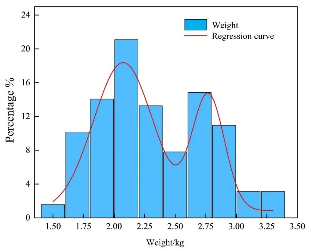
In the sample collection phase, this study selected multiple different breeds of broiler chickens for image capturing and weighing to ensure that the sample weights were distributed across a wider range, thereby avoiding data concentration and reducing the risk of model underfitting. A total of 165 broiler chicken samples were collected for weight data, and preliminary statistical analysis was conducted, as shown in
. According to the statistical results, the sample weights ranged from 1.55 kg to 3.35 kg, with an average weight of 2.29 kg and a median of 2.25 kg, exhibiting a relatively symmetric distribution pattern. The standard deviation is 0.44 kg, and the variance is 0.19 kg
2, indicating that the data has a moderate level of dispersion and no significant skewness.
.
Statistical Feature Analysis of Broiler Carcass Data.
| Count |
Max |
Min |
Median |
Average |
Standard |
Variance |
| 165 |
3.35 kg |
1.55 kg |
2.25 kg |
2.29 kg |
0.44 kg |
0.19 kg |
A histogram of broiler chicken carcass weight distribution was plotted based on weight, with the introduction of a kernel density estimation (KDE) curve to reflect the overall data trend (
). KDE [
30,
31] is a non-parametric method used to estimate the probability density function of a random variable. In the computational process, a smoothed kernel function, such as the commonly used Gaussian kernel, is applied around existing samples at each weight node [
32]. The integration of these local kernel functions ultimately forms a smooth and continuous probability density curve.
The calculation formula is as follows:
where, $$\hat{f} \left( x \right)$$ represents the density estimate at position $$x$$; $$n$$ is the sample size; $$h$$ is the bandwidth parameter; and $$K$$ is the kernel function.
. Broiler carcass weight distribution.
This study utilized the weighted histogram and KDE to conduct a visual analysis of the collected broiler chicken sample weight data. The results exhibit a clear bimodal distribution with peaks around 2.0 kg and 2.8 kg, which account for more than 65% of the samples. This aligns closely with the typical weight specifications of broiler chickens in the current market, further validating the market representativeness and reasonableness of the collected data.
After preliminarily extracting and classifying the broiler chicken carcass image features in Section 1, these features were further correlated with the actual weight data, followed by a detailed statistical sorting and selection process. Ultimately, five core features were identified, as shown in
. Among them, parameters such as the overall area (
Sp) and perimeter (
Hp) of the broiler chicken carcass are calculated from the whole chicken mask image, which can accurately depict the scale and boundary shape of the chicken carcass. The chicken breast area (
Ep) is derived from the manually labeled green mask region, reflecting the actual projected area of the chicken breast in the image.
.
Statistical analysis of broiler carcass pixel features and weight.
| No. |
Sp
(Pixels) |
Hp
(Pixels) |
Ep (Pixels) |
Cp (Pixels) |
Ap (Pixels) |
Wight
(kg) |
| AnnImg |
InfImg |
AnnImg |
InfImg |
AnnImg |
InfImg |
| 1 |
264,965 |
4367 |
133,698 |
124,016 |
483 |
445 |
236 |
233 |
3 |
| 2 |
255,727 |
4681 |
141,228 |
117,173 |
505 |
460 |
242 |
213 |
2.6 |
| 3 |
283,481 |
4254 |
182,643 |
232,868 |
611 |
627 |
258 |
310 |
2.45 |
| 4 |
243,050 |
3876 |
168,483 |
227,491 |
558 |
592 |
269 |
321 |
2.85 |
| 5 |
306,111 |
4040 |
200,099 |
237,275 |
848 |
658 |
394 |
301 |
3.1 |
| 6 |
282,094 |
3693 |
182,547 |
222,394 |
481 |
572 |
312 |
324 |
2.25 |
| 7 |
295,303 |
3650 |
201,014 |
159,459 |
652 |
501 |
281 |
266 |
2.75 |
| 8 |
331,866 |
4299 |
206,652 |
252,826 |
580 |
622 |
323 |
339 |
2.8 |
| 9 |
355,566 |
4377 |
246,388 |
212,404 |
689 |
639 |
317 |
277 |
2.9 |
| 10 |
256,370 |
3628 |
146,186 |
191,352 |
525 |
536 |
248 |
298 |
2.85 |
| 11 |
294,658 |
4268 |
180,890 |
143,691 |
606 |
528 |
275 |
227 |
2.25 |
| 12 |
298,186 |
4411 |
209,398 |
225,658 |
642 |
644 |
288 |
292 |
2.85 |
| 13 |
261,654 |
3900 |
176,208 |
239,078 |
564 |
601 |
295 |
332 |
2.95 |
| 14 |
345,002 |
4977 |
189,330 |
171,545 |
619 |
590 |
260 |
243 |
3 |
| 15 |
484,301 |
4968 |
327,403 |
297,030 |
753 |
754 |
367 |
329 |
2.85 |
| 16 |
367,469 |
4668 |
224,627 |
207,386 |
643 |
578 |
310 |
299 |
2.15 |
| 17 |
393,423 |
4447 |
255,372 |
198,608 |
917 |
631 |
426 |
263 |
3.35 |
| 18 |
289,799 |
4361 |
195,810 |
310,916 |
608 |
670 |
285 |
387 |
2.8 |
| 19 |
294,382 |
4035 |
180,843 |
244,669 |
598 |
687 |
265 |
297 |
2.7 |
| 20 |
192,055 |
3713 |
90892 |
168,035 |
440 |
251 |
189 |
140 |
2.05 |
4.2. Image Calibration
Image calibration maps three-dimensional physical coordinates to two-dimensional pixel coordinates through camera calibration and uses coordinate system transformation methods to establish the conversion relationship from the world coordinate system to the pixel coordinate system, typically represented by a matrix, as shown
.
where $$Z_{c}$$ represents depth, $$\begin{bmatrix} u & v & 1 \end{bmatrix}^{T}$$ denotes pixel coordinates; $$d_{x}$$ indicates the horizontal pixel size; $$d_{y}$$ represents the vertical pixel size is the lens focal length. The right side of the equation represents the camera’s intrinsic and extrinsic parameter matrices; $$\begin{bmatrix} x_{w} & y_{w} & z_{w} \end{bmatrix}^{T}$$ which represent the world coordinates. Camera calibration primarily involves solving the relevant parameters in the intrinsic and extrinsic matrices.
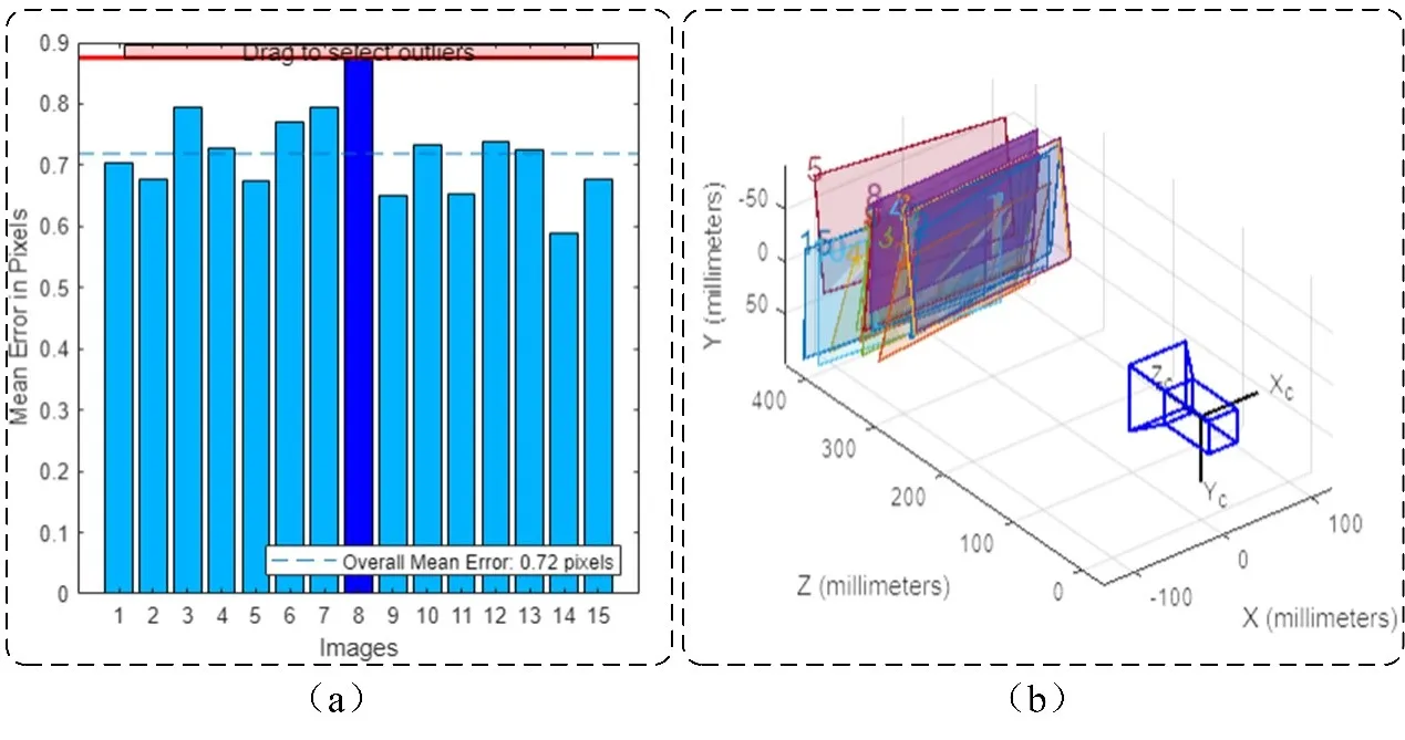
The internal parameter matrix obtained from camera calibration is denoted as $$K = \begin{bmatrix} 3301 . 2 & 0 & 1537 . 9 \\ 0 & 3305 . 7 & 2037 . 0 \\ 0 & 0 & 1 \end{bmatrix}$$; the distortion coefficients are $$k_{1}$$ = 0.0391 and $$k_{2}$$ = −0.3397.
Among them, a presents the error distribution in the form of a bar chart, with each bar reflecting the average error value corresponding to one calibrated image. From the perspective of the overall distribution, the errors of most images are concentrated around approximately 0.7 pixels, which reflects that the selected calibration method has strong controllability in terms of accuracy. In b, the 3D reconstruction results are presented with the help of internal and external parameters. After correcting the distortion phenomenon, the average error obtained is 0.72 pixels, and there is no situation where the error of a single image exceeds 1 pixel. This further indicates that this calibration has high accuracy and can meet the accuracy requirements of subsequent image measurement and 3D modeling.
. Camera calibration. (<b>a</b>) presents the error distribution in the form of a bar chart, with each bar reflecting the average error value corresponding to one calibrated image. (<b>b</b>), the 3D reconstruction results are presented with the help of internal and external parameters.
Through the aforementioned image calibration, the five feature quantities are converted from pixel units to physical units, with the ratio between the physical size and pixel size of the image remaining constant. That is:
where $$Q$$ is the scale factor, $$L_{r}$$ is the physical size (cm), and $$L_{p}$$ is the pixel size. The calculated value of $$Q$$ is 0.03838; thus, the physical calculation formula for this feature quantity is:
Sr,
Hr,
Er,
Cr, and
Ar represent the pixel unit values of the feature quantities corresponding to the overall area, perimeter, chest area, long axis, and short axis of the image, as obtained through image calibration. These pixel unit values of the feature quantities are obtained through the calibration process and are then converted into actual physical units.
presents the calculated results of the five data points in physical units obtained through the image feature conversion.
.
Statistical analysis of physical features and weight of broiler carcass.
| No. |
Sr (cm2) |
Hr (cm) |
Er (cm2) |
Cr (cm) |
Ar (cm) |
Weight (kg) |
| AnnImg |
InfImg |
AnnImg |
InfImg |
AnnImg |
InfImg |
| 1 |
390.29 |
167.60 |
196.94 |
182.67 |
9.27 |
8.53 |
4.53 |
4.46 |
3 |
| 2 |
376.69 |
179.66 |
208.03 |
172.60 |
9.68 |
8.82 |
4.63 |
4.08 |
2.6 |
| 3 |
417.57 |
163.28 |
269.03 |
343.01 |
11.72 |
12.03 |
4.95 |
5.94 |
2.45 |
| 4 |
358.01 |
148.77 |
248.17 |
335.09 |
10.71 |
11.35 |
5.15 |
6.15 |
2.85 |
| 5 |
450.90 |
155.04 |
294.75 |
349.51 |
11.43 |
12.63 |
5.61 |
5.77 |
3.1 |
| 6 |
415.52 |
141.73 |
268.89 |
327.59 |
9.22 |
10.98 |
5.98 |
6.22 |
2.25 |
| 7 |
434.98 |
140.07 |
296.09 |
234.88 |
12.51 |
9.60 |
5.38 |
5.09 |
2.75 |
| 8 |
488.84 |
164.98 |
304.40 |
372.41 |
11.13 |
11.93 |
6.19 |
6.51 |
2.8 |
| 9 |
523.75 |
167.98 |
362.93 |
312.87 |
13.21 |
12.26 |
6.07 |
5.32 |
2.9 |
| 10 |
377.63 |
139.25 |
215.33 |
281.86 |
10.07 |
10.29 |
4.75 |
5.71 |
2.85 |
| 11 |
434.03 |
163.82 |
266.45 |
211.66 |
11.62 |
10.12 |
5.28 |
4.36 |
2.25 |
| 12 |
439.23 |
169.29 |
308.44 |
332.39 |
12.31 |
12.36 |
5.52 |
5.60 |
2.85 |
| 13 |
385.42 |
149.70 |
259.55 |
352.16 |
10.82 |
11.53 |
5.65 |
6.36 |
2.95 |
| 14 |
508.19 |
191.02 |
278.88 |
252.69 |
11.88 |
11.31 |
4.98 |
4.65 |
3 |
| 15 |
713.38 |
190.65 |
482.26 |
437.52 |
14.44 |
14.46 |
7.04 |
6.30 |
2.85 |
| 16 |
541.28 |
179.17 |
330.87 |
305.48 |
12.34 |
11.09 |
5.94 |
5.74 |
2.15 |
| 17 |
579.51 |
170.69 |
376.16 |
292.55 |
13.31 |
12.10 |
6.04 |
5.04 |
3.35 |
| 18 |
426.87 |
167.36 |
288.43 |
457.98 |
11.66 |
12.85 |
5.46 |
7.43 |
2.8 |
| 19 |
433.62 |
154.86 |
266.38 |
360.40 |
11.48 |
13.17 |
5.09 |
5.70 |
2.7 |
| 20 |
282.90 |
142.49 |
133.88 |
247.52 |
8.44 |
9.61 |
3.62 |
5.36 |
2.05 |
Based on existing research, the body length of broiler chickens typically ranges from 35 to 45 cm, with the typical length of the chest area being 12 to 18 cm and the width ranging from 8 to 15 cm [
33,
34]. The main sources of uncertainty affecting the accuracy of the prediction results in this study include: image edge segmentation error (approximately 2.3% pixel deviation), camera calibration error (±0.13 cm), and weighing equipment error (±0.01kg). The total prediction uncertainty introduced by the combination of the three is approximately ±3.5%, which is within a reasonable range in non-contact detection tasks. By comparing the prediction results of the YOLO algorithm with the above typical values and reasoning data analysis, it is found that the output provided by this algorithm is highly consistent with the normal range.
4.4. Regression Prediction Model
Although traditional regression methods show some adaptability on the training set, their prediction performance is unstable when faced with unknown samples or validation data, which weakens their applicability in real-world scenarios. This paper aims to address these technical bottlenecks. Univariate linear regression can identify characteristics significantly correlated with chicken body weight, thereby reducing the interference of irrelevant information during the modeling process. Subsequently, multiple machine learning regression algorithms and convolutional neural network models are introduced to optimize predictive performance further. Finally, experiments are designed to compare the error differences between the predicted values of each model and the actual body weight, providing a comprehensive evaluation of the models’ accuracy and stability.
This chapter utilizes SPSS (Statistical Package for the Social Sciences) software to perform linear regression analysis and train traditional machine learning models, while using the MATLAB platform for the modeling and training of convolutional neural networks, thereby enabling further processing and predictive modeling of image features [
35].
To comprehensively evaluate the performance of the models, this study selects the coefficient of determination (
R2) and root mean square error (
RMSE) as evaluation metrics.
Where $$y$$ represents the actual observed value; $$\hat{y}$$ represents the model’s predicted value; and $$\overset{-}{y}$$ represents the mean of the actual values. The closer the
R2 value is to 1, the stronger the model’s predictive ability.
RMSE is used to measure the magnitude of the error between the model’s predicted results and the actual observed values. The formula for its calculation is as follows:
where $$X_{\mathrm{o b s} , i}$$ represents the
i-th actual observed value, $$X_{\mathrm{m o d e l} , i}$$ represents the
i-th model predicted value, and
n represents the sample size. A smaller
RMSE value indicates smaller prediction errors and higher accuracy of the model.
4.5. Linear Regression
Simple linear regression predicts by establishing a linear relationship between the dependent variable and one independent variable [
36]. The regression equation for the sample is assumed to be:
where $$W$$ is the predicted body weight, $$X$$ is the actual value of the feature, and
b, a are the coefficients to be determined. The least squares method was used to establish the simple linear regression model, resulting in 5 regression models. In this study, regression analyses were performed on the overall area
Sr, chicken chest area
Hr, perimeter
Er, long axis
Cr, and short axis
Ar, resulting in the corresponding regression equations and fitting results.
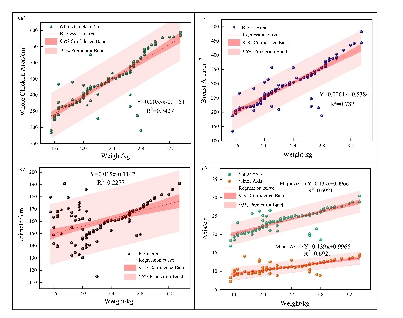
The results of the simple linear regression analysis are shown in
. Some features, such as the
R2 values of the perimeter and the short axis, are relatively low (e.g., 0.2277 and 0.6152, respectively). This can be attributed to their weak correlation with quality. These features are vulnerable to the influence of wing folding and background occlusion. Therefore, the model based on perimeter is not as reliable as the model based on area or axis. The discussion section explores these limitations and supports the selection of more stable features in model design. The whole body area and chest area of chickens have a strong linear correlation with the prediction of body weight, and the corresponding
R2 values are 0.7427 and 0.782, respectively. This indicates that these two characteristic variables have a high explanatory power for weight changes, and the regression model fits well.
.
Results of univariate linear regression analysis.
| Unit |
Regression Equation |
R2 |
| Whole Chicken Area |
$$W = 0 . 0055 S_{r} - 0 . 1151$$ |
0.7427 |
| Whole Chicken Perimeter |
$$W = 0 . 0 15 E_{r} - 0 . 11 42$$ |
0.2277 |
| Breast Area |
$$W = 0 . 0 061 H_{r} + 0 . 5384$$ |
0.7820 |
| Major Axis |
$$W = 0 . 139 C_{r} + 0 . 9966$$ |
0.6921 |
| Minor Axis |
$$W = 0 . 2512 A_{r} - 0 . 4689$$ |
0.6152 |
shows the linear modeling process of chicken body characteristics. It can be seen from the figure that the evaluation model is sensitive to the fluctuations of input features. In the regression prediction models of the overall area and chicken breast area, the predicted values fluctuated slightly, indicating that these two characteristics can accurately predict the body weight of chickens. However, the confidence interval and prediction interval of the perimeter are relatively wide, indicating that the error of this feature in weight prediction is large and the reliability of the prediction is low. It further explains that feature selection plays a key role in the stability of the model.
. Linear modeling based on broiler carcass feature values (<b>a</b>) Whole Chicken Area (<b>b</b>) Breast Area (<b>c</b>) Perimeter (<b>d</b>) Axis.
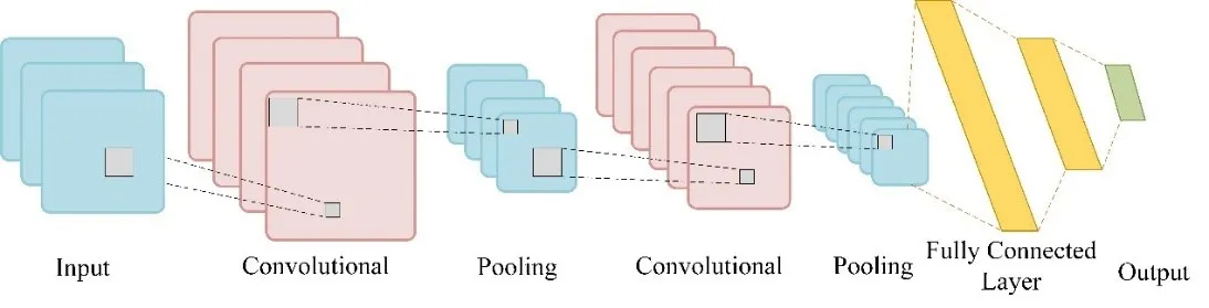
shows the CNN architecture used in this study. The model consists of an input layer, an output layer, and multiple convolutional layers, pooling layers, and fully connected layers [
37,
38,
39].
. Convolutional neural network structure diagram.
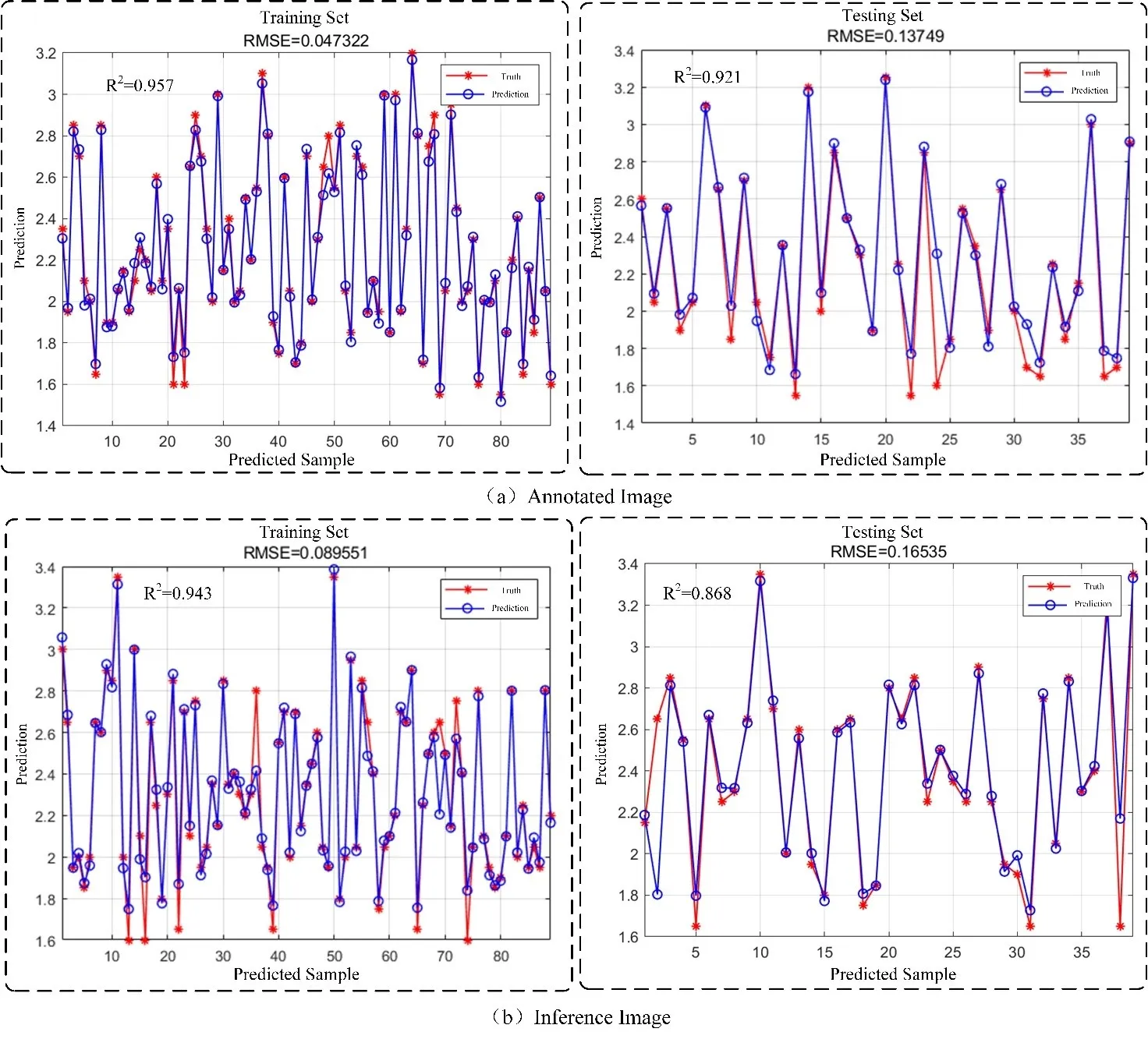
The extracted chicken body feature data was imported into the MATLAB environment. Prior to modeling, the data was randomly shuffled, and then the first 80 data points were selected as the training set, with the remaining samples used for testing and validating the model. The goal was to assess its generalization ability on unseen samples. The convolutional neural network was trained for a total of 2400 iterations. The CNN model training results are shown in the figure, where
a,b shows the comparison between the labeled and inferred images. For the training set data, the
R2 for labeled images was 0.957, and the
RMSE was 0.047; for inferred images, the
R2 was 0.921, and the
RMSE was 0.137. For the validation set data, the
R2 for labeled images was 0.943, and the
RMSE was 0.089; for inferred images, the
R2 was 0.868, and the
RMSE was 0.165.
. CNN model training results.
To validate the accuracy of the convolutional neural network regression, this study compares it with four other methods: Support Vector Machine Regression (SVR), Random Forest Regression (RF), Adaptive Boosting Regression, and Gradient Boosting Regression, to evaluate their performance in weight prediction [
40,
41,
42,
43,
44].
From the comparison of performance indicators in
, it can be seen that the SVR and Random Forest models achieved high fitting results on the labeled images of the training set, with
R2 values of 0.947 and 0.998, respectively, demonstrating strong modeling capabilities. However, when the models were applied to the inference images of the validation set, their performance significantly decreased, with
R2 dropping to around 0.8, reflecting the limited generalization ability of these two models when dealing with unseen data.
In contrast, the Adaptive Regression and Gradient Boosting Regression models showed more balanced prediction performance on both labeled and inference images. Especially on the validation set, their
R2 values were 0.904 and 0.856, respectively, indicating better stability and generalization performance. From the perspective of prediction error, the Gradient Boosting Regression model had a lower
RMSE, indicating that it has an advantage over Adaptive Regression in terms of prediction accuracy. Whether on labeled images or inference images, the Gradient Boosting model consistently showed more reliable regression results.
.
Prediction results of nonlinear models.
| Model |
Annotated Image |
Inferred Image |
| Training Set |
Validation Set |
Training Set |
Validation Set |
| R2 |
RMSE/kg |
R2 |
RMSE/kg |
R2 |
RMSE/kg |
R2 |
RMSE/kg |
| SVR |
0.947 |
0.066 |
0.811 |
0.142 |
0.955 |
0.094 |
0.806 |
0.103 |
| RF |
0.998 |
0.019 |
0.856 |
0.16 |
0.999 |
0.013 |
0.8 |
0.184 |
| Adboost |
0.935 |
0.114 |
0.904 |
0.116 |
0.881 |
0.154 |
0.824 |
0.171 |
| GBDT |
0.956 |
0.087 |
0.844 |
0.192 |
0.952 |
0.097 |
0.816 |
0.172 |
| CNN |
0.957 |
0.047 |
0.921 |
0.137 |
0.943 |
0.089 |
0.868 |
0.165 |
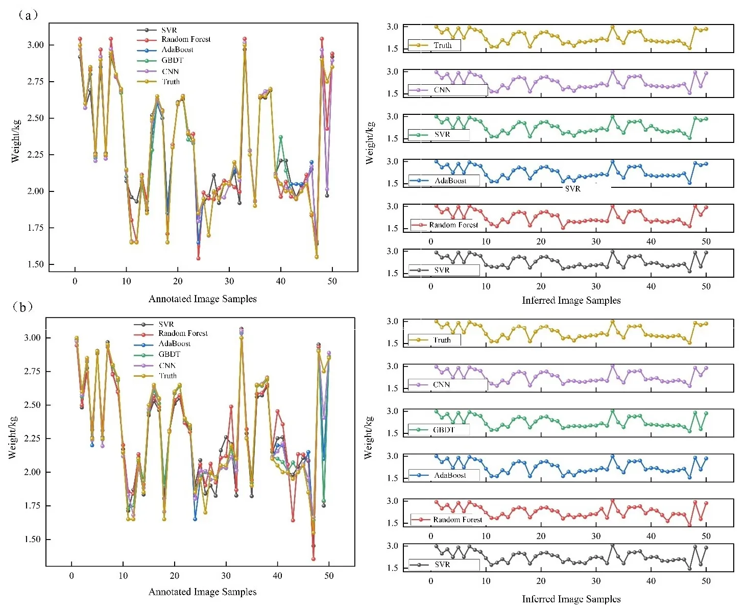
This study randomly selected 50 samples from the complete dataset for sample-level analysis and layered chart comparison, with the corresponding visualization results shown in
. Among them,
a and
b show the prediction effects of labeled images and inference images under different regression models, respectively. According to the analysis results in
,
a and
b respectively show the prediction effects of the labeled image and the inferred image under different regression models.CNN performed the best in the training set samples, with
R2 of 0.974 and
RMSE of 0.069, significantly outperforming other regression algorithms. In the validation set samples, CNN also maintained good performance, with
R2 of 0.953 and
RMSE of 0.093, indicating strong predictive ability and stability when dealing with unseen data. In contrast, the machine learning regression models showed relatively stable performance in the validation set, but their overall metrics were lower than CNN. Especially when facing complex features and unseen samples, CNN demonstrated stronger generalization ability and robustness through deep feature extraction.
The CNN model proposed in this study has a stronger generalization ability, integrates physical quantity calibration and deep learning, makes up for the defect of “only focusing on pixels and ignoring size” in traditional methods, and has higher interpretability and practicability in actual engineering deployment.
. (<b>a</b>,<b>b</b>) show prediction results of annotated and inference images by regression models.
.
Model prediction results.
| Model |
Annotated Image |
Inferred Image |
| R2 |
RMSE |
R2 |
RMSE |
| SVR |
0.812 |
0.189 |
0.776 |
0.211 |
| RF |
0.906 |
0.133 |
0.776 |
0.206 |
| Adboost |
0.958 |
0.089 |
0.911 |
0.130 |
| GBDT |
0.969 |
0.076 |
0.915 |
0.127 |
| CNN |
0.974 |
0.069 |
0.953 |
0.093 |
5. Intelligent Production Line for Broilers
Market research and analysis indicate that current poultry segmentation lines remain inefficient, with several unresolved technical challenges persisting in the cutting stage [
45,
46,
47,
48]. To address these issues, this study proposes the design of an intelligent segmentation production line for broilers. First, the overall framework of the production line was gradually established, and the process flow was clarified through detailed analysis. Second, key functional modules of the intelligent broiler segmentation line were developed, including a weighing and re-hanging unit, a machine vision-based wing extension detection unit, and an intelligent cutting system, each targeting specific technical bottlenecks. Finally, the practical application of the production line was evaluated, demonstrating its effectiveness in improving processing efficiency and optimizing workflow.
5.1. Intelligent Production Line Design
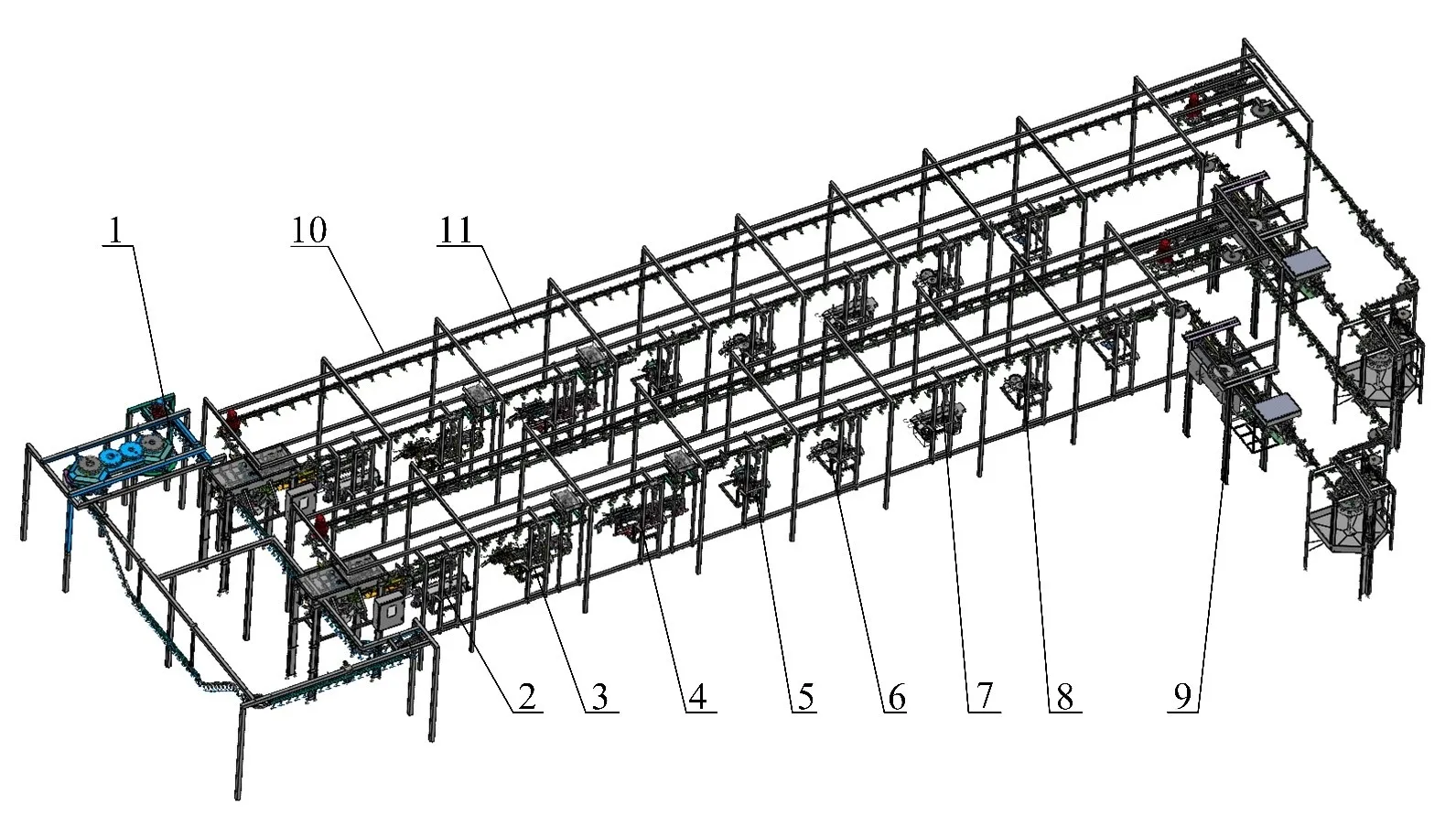
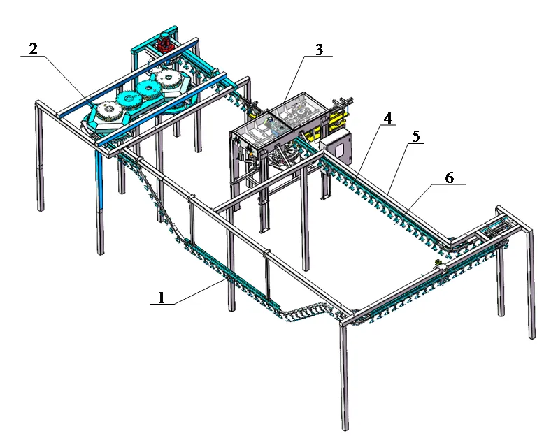
The intelligent broiler segmentation line is composed of a weighing and re-hanging unit, a vision-based wing-extension detection module, and an intelligent cutting system (
). The production line incorporates a dual-parallel conveyor hanging system, allowing broiler carcasses to remain stably suspended and smoothly transported along the line. The weighing and re-hanging unit is positioned at the beginning of the conveyor to ensure that each carcass enters the segmentation phase following standardized procedures. Downstream along the conveyor, the system is sequentially equipped with modules for wing-extension detection, followed by automated segmentation of the wing tip, mid-wing, wing root, neck, spine, breast cap, and leg portions, enabling a fully automated assembly-line operation.
. Layout of the intelligent poultry cutting production line. 1. Weighing and Re-Hanging 2. Machine Vision-Based Wing Extension Detection Module 3. Wing Tip Cutting 4. Mid-Wing Cutting 5. Wing Root Cutting 6. Breast Cap Segmentation Module 7. Poultry Neck Cutting 8. Spine Segmentation Module 9. Poultry Leg Cutting 10. Overhead Conveyor Rail 11. Production Line Frame.
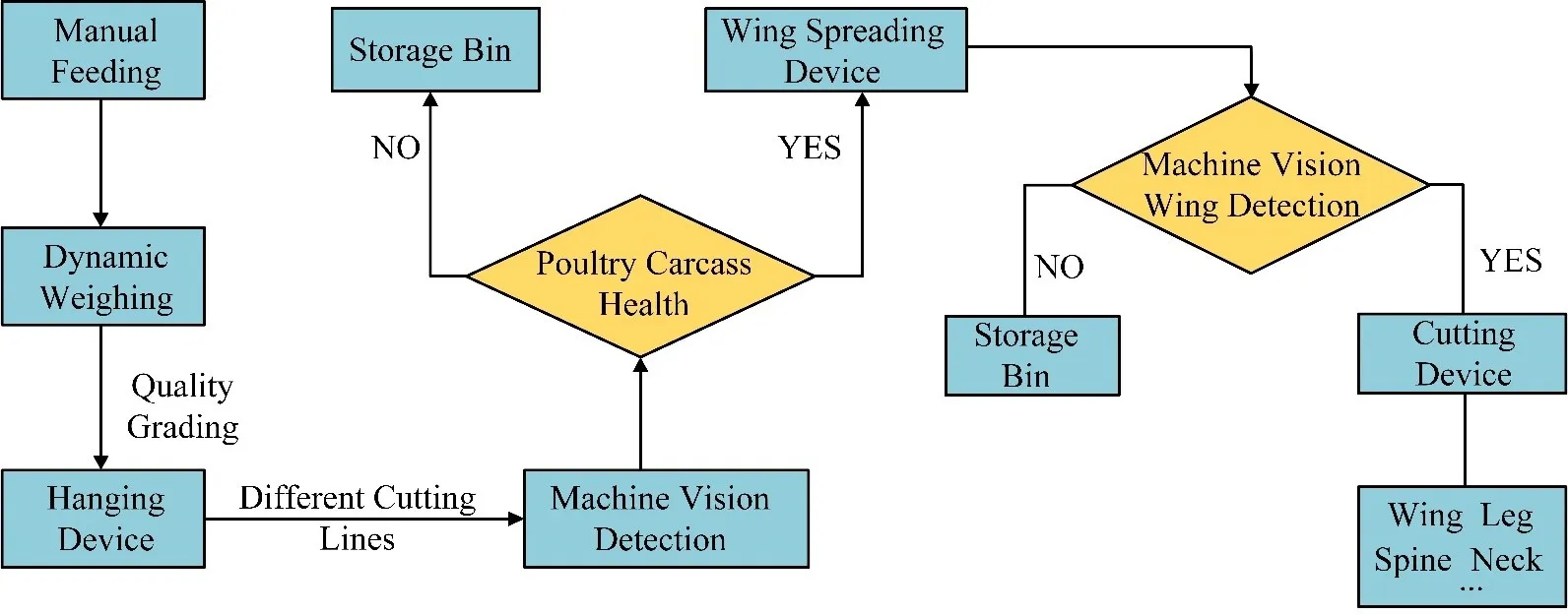
The operational workflow of the intelligent broiler segmentation line begins with Step 1: manually hanging broiler carcasses onto the weighing and transfer unit. As the conveyor rail advances, the carcasses enter the weighing system for preliminary grading. Based on the weight and physical specifications, each carcass is automatically routed to an appropriate segmentation line. Step 2: The carcasses are conveyed to the machine vision-based wing extension inspection module, which evaluates anatomical features, skin integrity, and the presence of any pathological signs. Carcasses, meeting the quality criteria, proceed to the wing extension unit. Upon completion of this stage, a secondary machine vision inspection confirms compliance with wing extension standards. Step 3: Carcasses that pass the wing extension inspection are sequentially transferred to the wing tip, mid-wing, wing root, breast cap, neck, spine, and leg cutting units. Each device performs precise cuts based on pre-configured parameters, ensuring a fully standardized and automated segmentation process. The detailed operational workflow of the intelligent broiler segmentation line is illustrated in
.
. Specific workflow of the intelligent poultry cutting production line.
The automatic grading and weighing transfer system in the intelligent broiler segmentation system (as shown in
) consists of the manual loading area, chain-based dynamic weighing structure, transfer unit, production line frame, conveyor track, and clamping devices. The dynamic weighing device is composed of the entry rotary wheel, exit rotary wheel, drive chain, guide rails, carriage, photoelectric switch, weighing sensors, bevel gears, support plate frame, carriage constraint plate, and weighing hooks. In the structural design, the top support plate frame is equipped with intermeshing bevel gear sets, while the bottom relies on the drive chain to connect the entry and exit rotary wheels. The carriage is firmly secured between the two rotary wheels by constraint plates. It is coordinated with the weighing hooks and the exit rotary device to ensure smooth transportation of the broiler carcasses after weighing. During the weighing process, the drive motor moves the entire mechanism via the chain. Integrated weighing sensors on the chain capture the carcass’s instantaneous weight. When the carriage approaches the photoelectric switch, the action is triggered, automatically completing data collection and recording tasks.
. Automatic classification weighing and transfer suspension system. 1. Manual Loading Area 2. Dynamic Weighing Structure 3. Transfer Device 4. Conveyor Track 5. Production Line Frame 6. Clamping Device.
The machine vision detection wing-spreading device (
) consists of a visual recognition component, an adaptive, flexible wing-spreading component, a side lifting frame, and a production line frame [
49].
. Adaptive flexible wing deployment mechanism 1. Pulling Plate 2. Guide Wheel Shaft 3. Motor Mounting Bracket 4. Motor 5. Bearing Mount 6. Lead Screw 7. Rubber Rod 8. Wing-Spreading Roller 9. Protective Cover 10. Gear Reduction Motor 11. Rhombic Bearing 12. Wing-Spreading Roller Base.
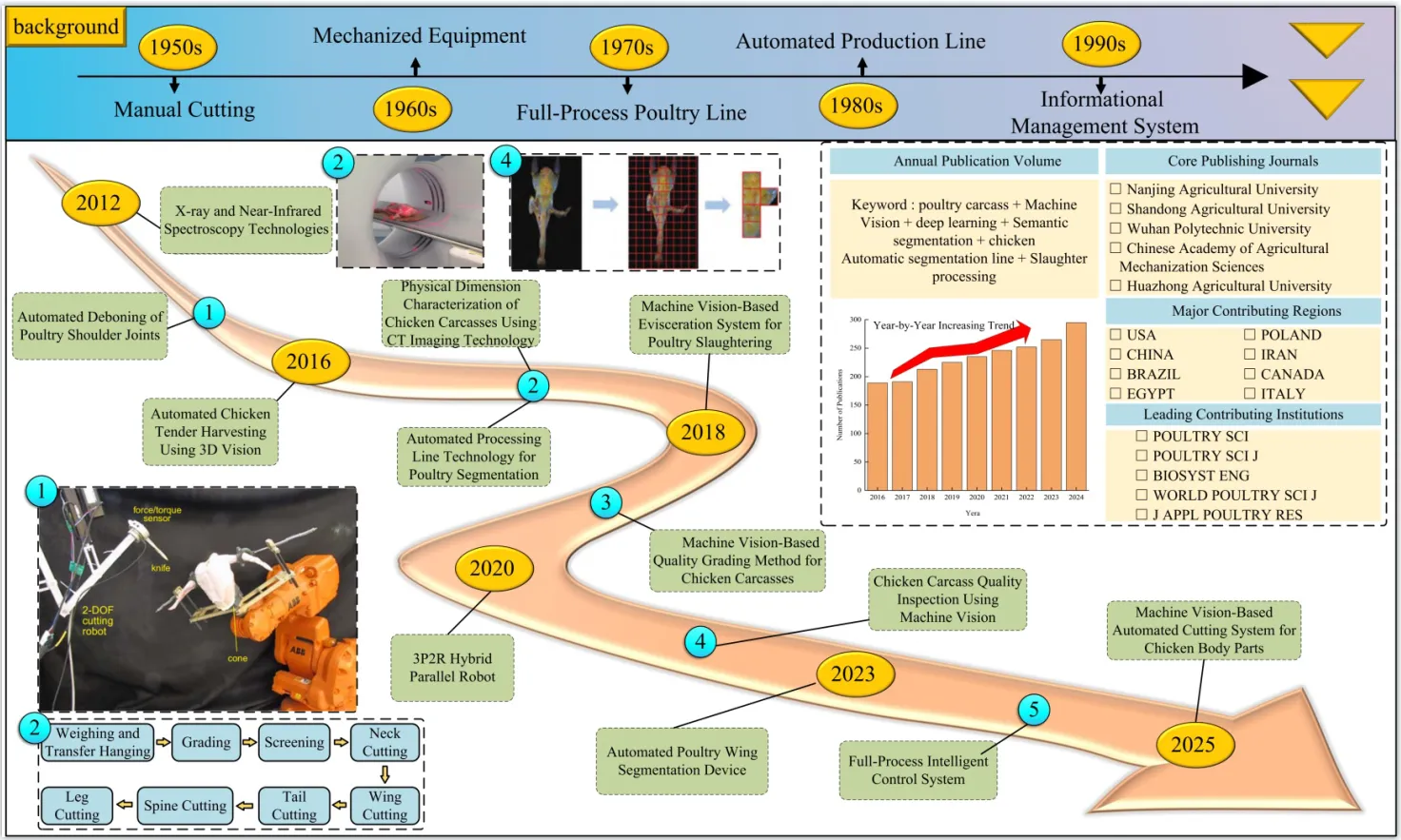
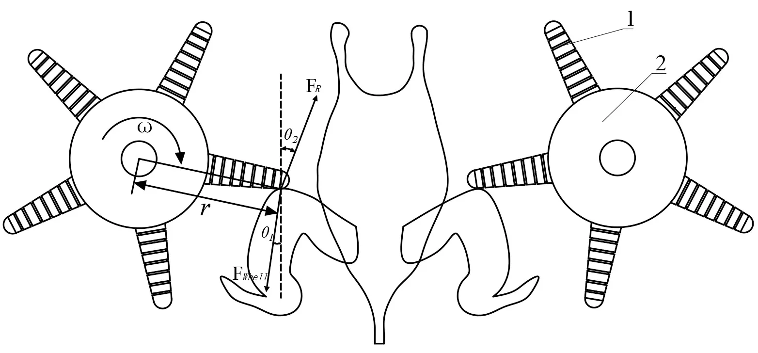
Throughout the process, the chicken body is suspended on the conveyor line’s rack, moving steadily in a fixed direction, with its posture pre-adjusted so that the chest faces forward, facilitating smooth transitions for subsequent operations. As the body gradually approaches the adaptive, flexible wing-spreading component, the naturally folded wings enter the wing-spreading space. As the body continues to move forward, its wings gradually come into contact with the rotating rubber rods. After several flexible impacts from the rubber rods, which differ from the force needed to maintain the wings’ contraction, the perfect reactive force is generated, causing the folded wings to gradually unfold and take shape, providing the optimal condition for the subsequent precise cutting process. When the body first enters the adaptive, flexible wing-spreading component (as shown in
), the force analysis at the contact point between the rubber rod and the chicken wings in their contracted state is shown below:
where, $$F_{\mathrm{W h e l l}}$$ represents the twisting force of the wing-spreading roller, in
N; $$F_{R}$$ represents the resistance exerted on the wing-spreading roller by the bird’s wing, in
N; the twisting force $$F_{\mathrm{W h e l l}}$$ generated by the rubber rod on the wing-spreading roller makes an angle of $$\theta_{1}$$,°; with the vertical direction; $$F_{R}$$ also makes an angle of $$\theta_{2}$$ with the vertical direction.
Let the rotational speed provided by the motor be
n, in rpm; the power transmitted by motor
P, in kW;
r is the distance between the rubber rod on the wing-spreading roller and the bird’s wing, in mm. The two motors drive the wing-spreading roller in opposite directions with the same rotational speed. Based on the relationship between torque
T, rotational speed
n, and power
P, in
W:
The twisting force $$F_{\mathrm{W h e l l}}$$ of the rubber rod is determined by the torque
T calculated above.
. Force analysis diagram of wing in contracted state. 1 Rubber rod 2 Winged roller.
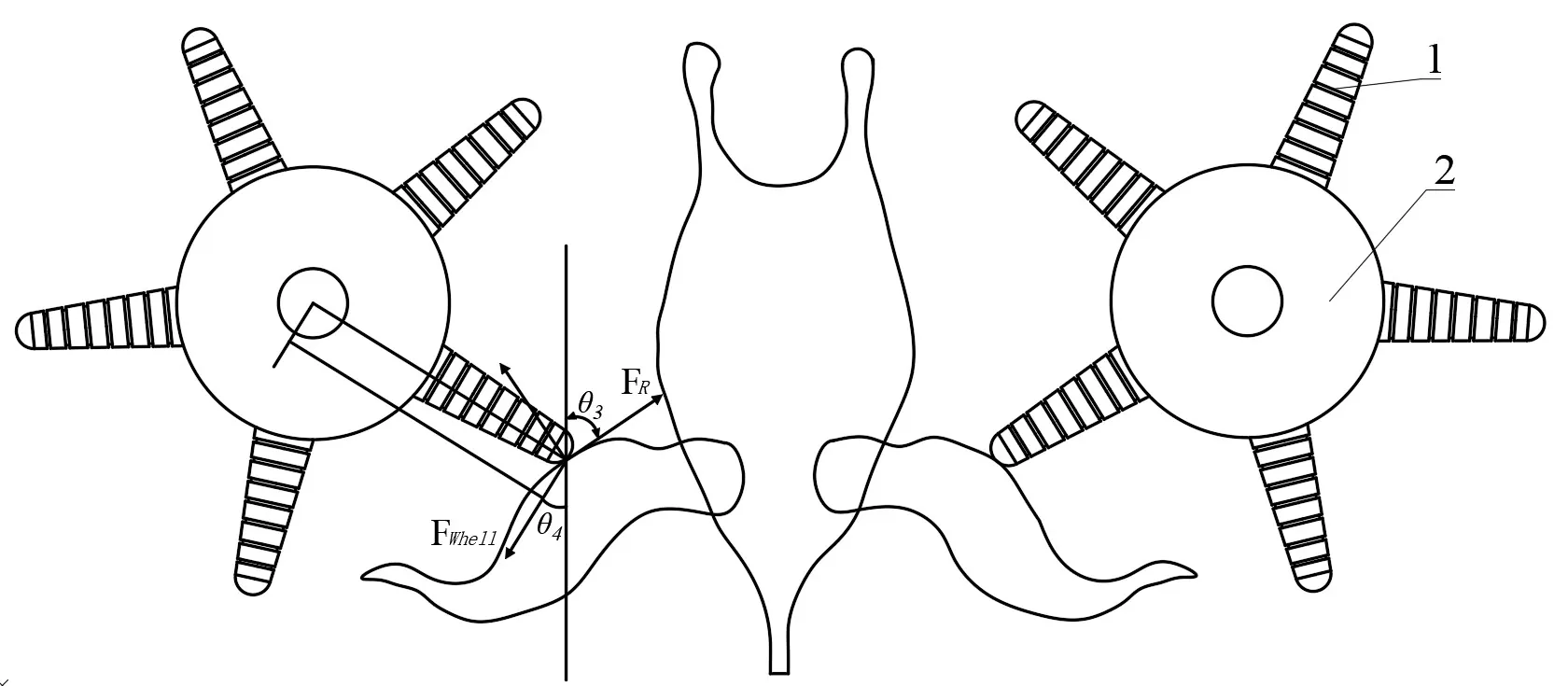
As shown in
, the forces acting on the broiler carcass wings in the fully extended state are illustrated. In the extended state, the torsional force acting on the wing forms an angle $$\theta_{3}$$ with the vertical direction, and the resistance force on the wing also forms an angle $$\theta_{4}$$ with the vertical. When the wings are fully extended, the length $$\theta_{3}$$ is reduced compared to $$\theta_{1}$$ in
, while the offset $$\theta_{4}$$ increases compared to $$\theta_{2}$$ in
. Therefore, the components of the torsional force $$F_{\mathrm{W h e l l}}$$ in both horizontal and vertical directions are greater than those of the resistance force $$F_{R}$$ acting on the wings. The rubber rods disengage from the wings, and the wings remain in the extended state when the following condition is satisfied:
. Force analysis diagram of wing in deployed state. 1 Rubber rod 2 Winged roller.
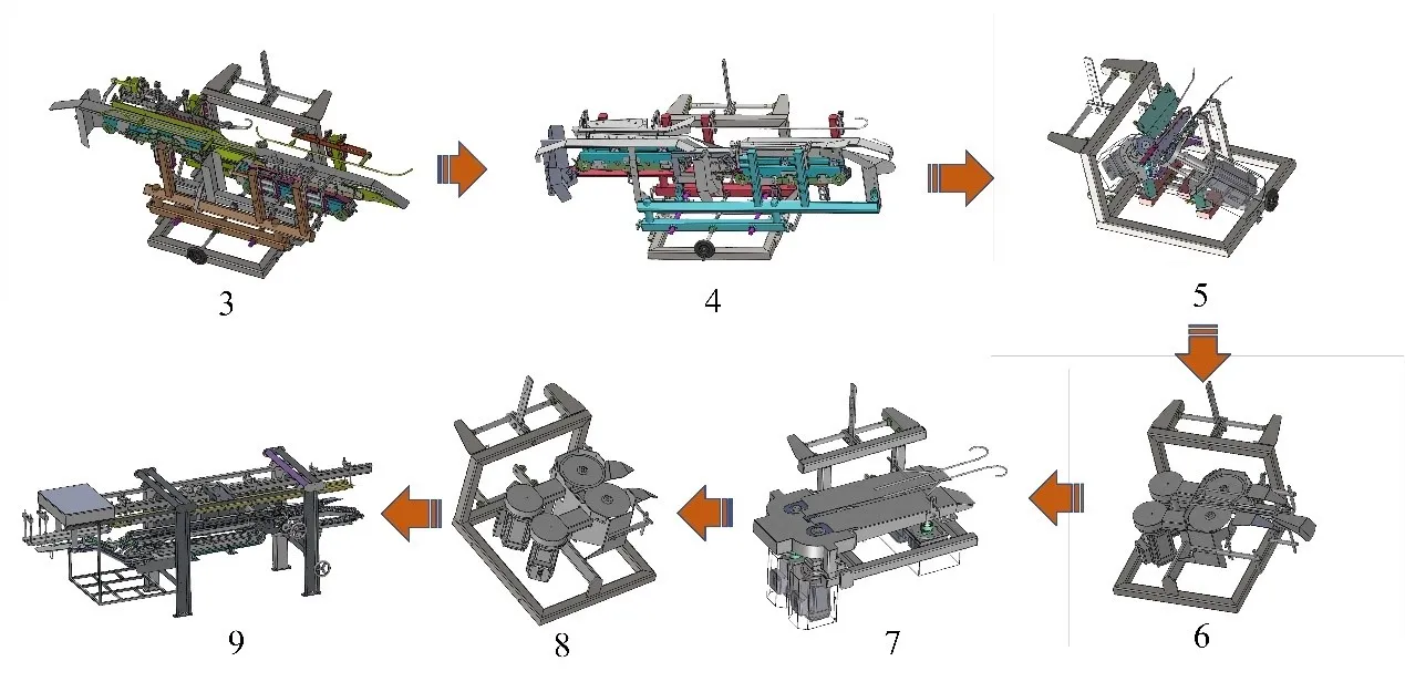
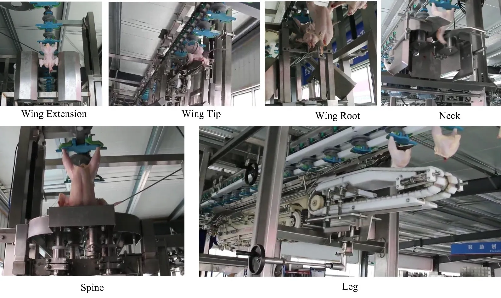
The cutting system precisely and sequentially cuts specific parts of broilers according to the pre-set cutting sequence, namely the wingtips, the middle of the wings, the neck, the wing roots, the spine and the legs. The equipment layout is strictly aligned with the cutting sequence. The horizontal support frame serves as the structural foundation to adjust the vertical position of the cutting unit. Once the position of the cutting module is relatively fixed, the system integrates the front-end machine vision recognition, the aforementioned automatic part discrimination and other functions. For instance, the system can identify whether chicken wings have spread out, adjust the cutting strategy based on the detection results, achieve cutting prediction and then precise cutting, truly realizing self-adaptation and automation.
shows the intelligent broiler cutting system.
. Poultry intelligent cutting system. 3. Wing Tip Cutting 4. Mid-Wing Cutting 5. Wing Root Cutting 6. Breast Cap Segmentation Module 7. Poultry Neck Cutting 8. Spine Segmentation Module 9. Poultry Leg Cutting.
This intelligent broiler segmentation line was jointly developed through an industry-university-research collaboration between Qingdao University of Technology and Qingdao Ruizhi Intelligent Technology Co., Ltd., Qingdao, China. The system has been deployed in actual production (as shown in
) and is currently operating with stable performance.
The intelligent broiler processing line features advanced automation, high reliability, and integrated information-sharing capabilities. By leveraging machine vision technology to identify broiler features, the system ensures accurate segmentation across more than 40 processing steps. It achieves high-precision separation of wing tips, mid-wings, and wing roots, increasing the wing-cutting efficiency to 4 kg/min. The joint breakage rate during bone-in component separation has been reduced to 5%. Furthermore, the broiler component processing equipment has achieved 100% interconnectivity, including 100% real-time data acquisition for both power consumption and production processes. This enables full lifecycle information tracking and integration of key resources throughout the broiler processing workflow. The system also incorporates intelligent predictive maintenance, optimizing production parameters based on historical and real-time sensor data. This framework supports a production optimization and control platform. As a result, the equipment failure rate has decreased by 11.38%, and overall operational efficiency has improved by more than 3%.
. Poultry intelligent segmentation production line application.
6. Conclusions
- 1.
-
For the demand for meat chicken carcass image segmentation accuracy and model running efficiency in assembly line scenarios, this study proposes a lightweight image segmentation model based on the improved YOLOv8n-seg, incorporating the latest SAM technology for high-quality semantic annotation of the meat chicken carcass dataset, thus improving the accuracy of training data from the source. In terms of network structure, the improved model integrates the ADown downsampling module, achieving a significant reduction in computational overhead while maintaining detection accuracy close to the baseline model (mAP@0.5 of 99.2% and 99.4%, respectively). This leads to a reduction in total parameters by 0.5 M (to 2.8 M), a decrease in floating-point operations by 0.9 G (to 11.1 G), and a reduction in model weight volume by 7.51 M (to 5.39 M). The improvement effectively reduces the storage and computational burden of the model in actual deployment, providing a feasible technical solution for real-time segmentation applications on embedded terminals.
- 2.
-
After comparing the effects of various image processing techniques, it was found that the HSV color space conversion, convex hull contours, and improved ellipse fitting algorithm have advantages in extracting carcass geometric features. Without preprocessing steps, the area and perimeter data of the carcass region often show significant deviations, affecting the accuracy of subsequent features. Introducing the HSV color space can significantly reduce the interference caused by background clutter, ensuring data stability (area of 319,377 pixels, perimeter of 5439.61 pixels). The chicken breast region extraction introduces the convex hull algorithm, optimizing the mask boundary and greatly reducing morphological deviation. The processed mask has the lowest relative error, nearly 4.0%, while the ellipse fitting calculation also shows very small deviations in the long and short axes, with approximately 0.6% deviation in the long axis and 1.2% deviation in the short axis, making the results closely fit the actual breast shape.
- 3.
-
Based on image calibration technology, the pixel features are converted to physical values, and the collected carcass feature data is used to construct linear and nonlinear regression models. Regression prediction is performed using univariate linear regression, SVR, random forest regression, adaptive boosting regression, gradient boosting regression, and CNN to construct models. Experimental results show that the gradient boosting regression model achieves R2 of 0.969 (RMSE = 0.076) on the training set and R2 of 0.915 (RMSE = 0.127) on the validation set. Meanwhile, the CNN model’s R2 increases to 0.974 and 0.953 on the training and validation sets, respectively, with RMSE decreasing to 0.069 and 0.093, fully demonstrating the clear advantage of deep learning in predicting the quality of meat chicken carcasses.
- 4.
-
An intelligent broiler segmentation production line integrating a weighing and transfer device, machine vision-based wing extension detection module, and intelligent cutting system has been developed. In practical applications, the production line has achieved efficient execution of more than 40 standardized cutting procedures. The processing efficiency of wing parts has increased to 4 kg/min. The damage rate for bone-in joint cutting has been reduced to 5%. In addition, the system has achieved 100% data acquisition coverage. The equipment failure rate has decreased by 11.38%, and the overall operational efficiency has improved by more than 3% compared to the original system.
7. Prospect
- 1.
-
On the basis of ensuring segmentation accuracy, future research can focus on optimizing the lightweight design of the network structure and moderately reducing the complexity of the model and the computational burden. Meanwhile, the online learning mechanism and adaptive segmentation method are introduced to enable the model to have the ability of real-time update and dynamic adjustment, which can respond more flexibly to the morphological changes and environmental disturbances of different batches of broilers in actual production. Integrating infrared, depth maps, and other multi-source sensing data together will significantly enhance the robustness of target recognition and the comprehensiveness of feature extraction.
- 2.
-
The current quality prediction models are mainly based on image feature extraction and have not fully considered spatial dimension information such as thickness and contour key points. In future research, more detailed parameters may be introduced, such as the thickness of broilers and three-dimensional contour data of certain parts, and actual variables, such as the actual width and length values of chicken wings and chicken legs, can be integrated, thereby generating a more refined quality assessment system. With the gradual deepening of the segmentation parameter prediction link, the automatic adjustment ability of the equipment can also be optimized and driven from it, and the dynamic adaptation of the entire system can be completed by continuously strengthening the feedback closed-loop performance.
- 3.
-
Although this study proposed a relatively reasonable production line layout scheme, during the cutting process, broiler carcasses inevitably come into frequent contact with equipment, tools, and environmental surfaces, and the hidden concern of cross-contamination is particularly difficult to ignore. In the future, it can be considered to deeply integrate new sterilization technologies (such as ozone sterilization, heat treatment, ultraviolet disinfection, etc.) with intelligent control systems, explore the linkage mechanism of multiple disinfection methods, optimize the sterilization process and parameter Settings, and thereby achieve a more efficient and environmentally friendly disinfection solution for production lines.
Author Contributions
Conceptualization, Z.H. and C.L.; Methodology, Y.H.; Software, M.C. and C.D.; Validation, J.G., Z.Y. and X.W.; Investigation, Z.H.; Data Curation, C.L.; Writing—Original Draft Preparation, Z.H.; Writing—Review & Editing, C.L.; Supervision, Y.Z., H.W., Y.S. and X.G.; Funding Acquisition, C.L.
Ethics Statement
Not applicable.
Informed Consent Statement
Not applicable.
Funding
This study was financially Supported by National Natural Science Foundation of China (52375447), the Special Fund of Taishan Scholars Project, the Shandong Province Youth Science and Technology Talent Support Project (Grant No.SDAST2024QTA043), and the Open Funding of Key Lab of Industrial Fluid Energy Conservation and Pollution Control, Ministry of Education (Grant Nos. CK-2024-0031, CK-2024-0035 and CK-2024-0036).
Declaration of Competing Interest
The authors declare that they have no known competing financial interests or personal relationships that could have appeared to influence the work reported in this paper.
References
-
1.
Xin XF, Zheng MQ, Wen J, Wang JM. Analysis of the Situation of China’s Broiler Industry in 2023, Future Outlook and Countermeasures and Suggestions.
Xumu Shouyi Xuebao 2024,
60, 312–317. doi:10.19556/j.0258-7033.20240131-10.
[Google Scholar]
-
2.
Abbas AO, Nassar FS, Al Ali AM. Challenges of Ensuring Sustainable Poultry Meat Production and Economic Resilience under Climate Change for Achieving Sustainable Food Security.
Res. World Agric. Econ. 2025,
6, 159–171. doi:10.36956/rwae.v6i1.1441.
[Google Scholar]
-
3.
Chen KJ, Li H, Yu ZW, Bai LF. Grading of Chicken Carcass Weight Based on Machine Vision.
Trans. Chin. Soc. Agric. Mach. 2017, 48, 290–295+372.
[Google Scholar]
-
4.
Qi C, Xu JQ, Liu C, Wu QM, Chen KJ. Automatic classification of chicken carcass weight based on machine vision and machine learning technology.
J. Nanjing Agric. Univ. 2019,
42, 551–558. doi:10.7685/jnau.201808013.
[Google Scholar]
-
5.
Ding XL, Wu YH, Zhou TT, Zuo RG, Guo YG, Zhao LX. Chicken wing quality prediction based on machine vision technology.
Jiangsu Agric. Sci. 2017,
45, 208–212. doi:10.15889/j.issn.1002-1302.2017.09.057.
[Google Scholar]
-
6.
Zhuang C, Shen MX, Liu LS, Yao W, Zheng HH, Wang MY. Weight estimation model of breeding chickens based on neural network and machine learning.
J. China Agric. Univ. 2021,
26, 107–114. doi:10.11841/j.issn.1007-4333.2021.07.11.
[Google Scholar]
-
7.
Nyalala I, Okinda C, Makange N, Korohou T, Chao Q, Nyalala L, et al. On-line weight estimation of broiler carcass and cuts by a computer vision system.
Poult. sci. 2021,
100, 101474. doi:10.1016/j.psj.2021.101474.
[Google Scholar]
-
8.
Wu JC, Wang HH, Xu XL. Rapid detection technology for chicken carcass wing breakage based on machine vision.
Trans. Chin. Soc. Agric. Eng. 2022,
38, 253261. doi:10.11975/j.issn.1002-6819.2022.22.027.
[Google Scholar]
-
9.
Wu JC, Wang HH, Xu XL. Rapid Machine Vision Method for Detection of Primary Dermatitis in Broiler Carcass.
Food Sci. 2023,
44, 350–356. doi:10.7506/spkx1002-6630-20221010-084.
[Google Scholar]
-
10.
Zhao ZD, Wang HH, Xu XL. Broiler carcass congestion detection technology using machine vision.
Trans. CSAE 2022,
38, 330–338. doi:10.11975/j.issn.1002-6819.2022.16.036.
[Google Scholar]
-
11.
Tran M, Truong S, Fernandes AF, Kidd MT, Le N. CarcassFormer: an end-to-end transformer-based framework for simultaneous localization, segmentation and classification of poultry carcass defect.
Poult. Sci. 2024,
103, 103765. doi:10.1016/j.psj.2024.103765.
[Google Scholar]
-
12.
Chen Y, Peng X, Cai L, Jiao M, Fu D, Xu CC, et al. Research on automatic classification and detection of chicken parts based on deep learning algorithm.
J. Food Sci. 2023,
88, 4180–4193. doi:10.1111/1750-3841.16747.
[Google Scholar]
-
13.
Xiao MZ, Zhang ZH, Liu WX, Zhong L. A Chicken Part Segmentation Method Based on CP-U Net.
Comput. Digit. Eng. 2024,
52, 1516–1522. doi:10.3969/j.issn.1672-9722.2024.05.044.
[Google Scholar]
-
14.
Hu A-P, Bailey J, Matthews M, McMurray G, Daley W. Intelligent automation of bird deboning. In Proceedings of the 2012 IEEE/ASME International Conference on Advanced Intelligent Mechatronics (AIM), Kaohsiung, China, 11–14 July 2012; pp. 286–291.
-
15.
Misimi E, Øye ER, Eilertsen A, Mathiassen JR, Åsebø OB, Gjerstad T. GRIBBOT–Robotic 3D vision-guided harvesting of chicken fillets.
Comput. Electron. Agric. 2016,
121, 84–100. doi:10.1016/j.compag.2015.11.021.
[Google Scholar]
-
16.
Ahlin K. The robotic workbench and poultry processing 2.0.
Anim. Front. 2022,
12, 49–55. doi:10.1093/af/vfab079.
[Google Scholar]
-
17.
Yu Z, Wan L, Yousaf K, Lin H, Zhang J, Jiao H, et al. An enhancement algorithm for head characteristics of caged chickens detection based on cyclic consistent migration neural network.
Poult. Sci. 2024,
103, 103663. doi:10.1016/j.psj.2024.103663.
[Google Scholar]
-
18.
Mehdizadeh SA, Siriani ALR, Pereira DF. Optimizing Deep Learning Algorithms for Effective Chicken Tracking through Image Processing.
AgriEngineering 2024,
6, 2749–2767. doi:10.3390/agriengineering6030160.
[Google Scholar]
-
19.
Wang C-Y, Yeh I-H, Mark Liao H-Y. Yolov9: Learning what you want to learn using programmable gradient information. In European Conference on Computer Vision; Springer Nature: Cham, Switzerland, 2024; pp. 1–21.
-
20.
Kirillov A, Mintun E, Ravi N, Mao H, Rolland C, Gustafson L. Segment anything. In Proceedings of the IEEE/CVF International Conference on Computer Vision, Paris, France, 2–3 October 2023; pp. 4015–4026.
-
21.
Li F, Xue M, Zhan Y, Yang Y. Semantic segmentation of 3D real scene based on segment anything model.
Bull. Surv. Map. 2024,
12, 101–105. doi:10.13474/j.cnki.11-2246.2024.1216.
[Google Scholar]
-
22.
Sun X, Dong L, Liu Z, Qin A, Liu J, Zhou Z, et al. Intelligent Manufacturing of a Bibliometric Review: From Frontier Hotspots to Key Technologies and Applications.
Chin. J. Mech. Eng. 2025,
38, 176. doi:10.1186/s10033-025-01274-y.
[Google Scholar]
-
23.
Kim S, You J. Efficient LUT design methodologies of transformation between RGB and HSV for HSV based image enhancements.
J. Electr. Eng. Technol. 2024,
19, 4551–4563. doi:10.1007/s42835-024-01859-y.
[Google Scholar]
-
24.
Panhu L. The Improved Retinex Algorithm Based on the HSV Color Space: Achieving Efficient Low-Light Image Enhancement and Color Fidelity. In Proceedings of the 14th International Conference on Information Technology in Medicine and Education (ITME), Guiyang, China, 13–15 September 2024; pp. 299–304. doi:10.1109/ITME63426.2024.00068.
-
25.
Güzel BC, Manuta N, Ünal B, Ruzhanova-Gospodinova IS, Duro S, Gündemir O, et al. Size and shape of the neurocranium of laying chicken breeds.
Poult. Sci. 2024,
103, 104008. doi:10.1016/j.psj.2024.104008.
[Google Scholar]
-
26.
Zhu R, Li J, Yang J, Sun R, Yu K.
In Vivo Prediction of Breast Muscle Weight in Broiler Chickens Using X-ray Images Based on Deep Learning and Machine Learning.
Animals 2024,
14, 628. doi:10.3390/ani14040628.
[Google Scholar]
-
27.
Campbell M, Miller P, Díaz-Chito K, Irvine S, Baxter M, Del Rincón JM, et al. Automated precision weighing: leveraging 2D video feature analysis and machine learning for live body weight estimation of broiler chickens.
Smart Agric. Technol. 2025,
10, 100793. doi:10.1016/j.atech.2025.100793.
[Google Scholar]
-
28.
Shams MY, Elmessery WM, Oraiath AAT, Elbeltagi A, Salem A, Kumar P, et al. Automated On-site Broiler Live Weight Estimation Through YOLO-Based Segmentation.
Smart Agric. Technol. 2025,
10, 100828. doi:10.1016/j.atech.2025.100828.
[Google Scholar]
-
29.
Zhao C, Zou K, Xu LY, Wu H. Error Analysis of Ellipse Fitting for Incomplete Contour.
J. Donghua Univ. 2024,
41, 323–332. doi:10.19884/j.1672-5220.202309003.
[Google Scholar]
-
30.
Li Z, Cao B, Peng D, You Q, Miao X, Chen Z. Inversion of nuclear accident source terms combining Bayesian method with machine learning.
Ann. Nucl. Energy 2025,
218, 111418. doi:j.anucene.2025.111418.
[Google Scholar]
-
31.
Abdel-Basset M, Mohamed R, Abouhawwash M. Crested Porcupine Optimizer: A new nature-inspired metaheuristic.
Knowl. -Based Syst. 2024,
284, 111257. doi:10.1016/j.knosys.2023.111257.
[Google Scholar]
-
32.
Moreo A, González P, del Coz JJ. Kernel density estimation for multiclass quantification.
Mach. Learn. 2025,
114, 92. doi:10.1007/s10994-024-06726-510.
[Google Scholar]
-
33.
Wang J, Liu J, Lei Q, Liu Z, Han H, Zhang S, et al. Elucidation of the genetic determination of body weight and size in Chinese local chicken breeds by large-scale genomic analyses.
BMC Genom. 2024,
25, 296. doi:10.1186/s12864-024-10185-6.
[Google Scholar]
-
34.
Song Y-X, Li C-H, Zhou Z-M, Liu B, Sharma S, Dambatta YS. Nanobiolubricant grinding: A comprehensive review.
Adv. Manuf. 2025,
13, 1–42. doi:10.1007/s40436-023-00477-7.
[Google Scholar]
-
35.
Huang Z, Li C, Zhou Z, Liu B, Zhang Y, Yang M. Magnetic bearing: structure, model, and control strategy.
Int. J. Adv. Manuf. Technol. 2024,
131, 3287–3333. doi:10.1007/s00170-023-12389-8.
[Google Scholar]
-
36.
Cai M, Li X, Liang J, Liao M, Han Y. An effective deep learning fusion method for predicting the TVB-N and TVC contents of chicken breasts using dual hyperspectral imaging systems.
Food Chem. 2024,
456, 139847. doi:10.1016/j.foodchem.2024.139847.
[Google Scholar]
-
37.
Jifang L, Xiangyang Z, Min L, Shuqing H, Leifeng G, Liang C. Artificial Intelligence-Driven High-Quality Development of New-Quality Productivity in Animal Husbandry: Restraining Factors, Generation Logic and Promotion Paths.
Smart Agric. 2025,
7, 165. doi:10.12133/j.smartag.SA202407010.
[Google Scholar]
-
38.
Wang X, Wei Q, Mu Y, Sheng Q, Yang L, An J. Research Progress of Swine Body Mass Estimation Based on Machine Vision.
J. Henan Agric. Sci. 2024,
53, 17. doi:10.15933/j.cnki.1004-3268.2024.11.002.
[Google Scholar]
-
39.
Triyanto WA, Adi K, Suseno JE. Indoor Location Mapping of Lameness Chickens with Multi Cameras and Perspective Transform Using Convolutional Neural Networks.
Math. Model. Eng. Probl. 2024,
11, 543. doi:10.18280/mmep.110227.
[Google Scholar]
-
40.
Qi H, Li C, Huang G. Dead chicken target detection algorithm based on lightweight YOLOv4.
J. Chin. Agric. Mech. 2024,
45, 195. doi:10.13733/j.jcam.issn.2095-5553.2024.05.030.
[Google Scholar]
-
41.
Sun S, Wei L, Chen Z, Chai Y, Wang S, Sun R. Nondestructive estimation method of live chicken leg weight based on deep learning.
Poult. Sci. 2024,
103, 103477. doi:10.1016/j.psj.2024.103477.
[Google Scholar]
-
42.
Wang K, Li Z, Wang C, Guo B, Li J, Lv Z, et al. Research and Design of a Chicken Wing Testing and Weight Grading Device.
Electronics 2024,
13, 1049. doi:10.3390/electronics13061049.
[Google Scholar]
-
43.
Peng X, Xu C, Zhang P, Fu D, Chen Y, Hu Z. Computer vision classification detection of chicken parts based on optimized Swin-Transformer.
CyTA-J. Food 2024,
22, 2347480. doi:10.1080/19476337.2024.2347480.
[Google Scholar]
-
44.
Chen R, Zhao Y, Yang Y, Wang S, Li L, Sha X, et al. Online estimating weight of white Pekin duck carcass by computer vision.
Poult. Sci. 2023,
102, 102348. doi:10.1016/j.psj.2022.102348.
[Google Scholar]
-
45.
Chen M, Zhang Y, Liu B, Zhou Z, Zhang N, Wang H. Design of intelligent and sustainable manufacturing production line for automobile wheel hub.
Intell. Sustain. Manuf. 2024,
1, 10003.
[Google Scholar]
-
46.
Liu D, Liu H, Zhou Z, Chen Y, Liu B, Zhang N. Design and Analysis of Flexible Fixture for Aluminum Alloy Hub.
Tool Eng. 2022,
56, 75–82. doi:10.3969/j.issn.1000-7008.2022.10.014.
[Google Scholar]
-
47.
Zhang Y, Sun L, Xu S, Zhao Y, Xu W, Li C. Design of intelligent clean manufacturing line for torque converter housing.
Manuf. Technol. Mach. Tool 2024,
08, 16–25. doi:10.19287/j.mtmt.1005-2402.2024.08.002.
[Google Scholar]
-
48.
Suleiman D Y, Li Q, Li B, Zhang Y, Zhang B, Liu D. Digital Twin and Artificial Intelligence in Machining: A Bibliometric Analysis.
Intell. Sustain. Manuf. 2025,
2, 10005. doi:10.19287/j.mtmt.1005-2402.2024.08.002.
[Google Scholar]
-
49.
Huang Z, Li C, Zhang Y, Cao M, Wang J. A Wing-Spreading Device and Method Based on Machine Vision Recognition. CN118556734A, 30 August 2024.